Benchmark of the Modular High-Temperature Gas-Cooled

Nuclear Science NEA/NSC/R(2017)4 February 2018 www.oecd-nea.org

Benchmark of the ModularHigh-Temperature Gas-Cooled Reactor (MHTGR)-350 MW Core Design

Volumes I and II

anni ve r

s ar y

NEAth

NUCLEAR ENERGY AGENCY

NEA/NSC/R(2017)4

1

NEA Benchmark of the Modular High-Temperature Gas-Cooled Reactor-350 MW Core Design

Volumes I and II

NEA/NSC/R(2017)4

2

ORGANISATION FOR ECONOMIC CO-OPERATION AND DEVELOPMENT

The OECD is a unique forum where the governments of 35 democracies work together to address the economic, social and environmental challenges of globalisation. The OECD is also at the forefront of efforts to understand and to help governments respond to new developments and concerns, such as corporate governance, the information economy and the challenges of an ageing population. The Organisation provides a setting where governments can compare policy experiences, seek answers to common problems, identify good practice and work to co-ordinate domestic and international policies.

The OECD member countries are: Australia, Austria, Belgium, Canada, Chile, the Czech Republic, Denmark, Estonia, Finland, France, Germany, Greece, Hungary, Iceland, Ireland, Israel, Italy, Japan, Korea, Latvia, Luxembourg, Mexico, the Netherlands, New Zealand, Norway, Poland, Portugal, the Slovak Republic, Slovenia, Spain, Sweden, Switzerland, Turkey, the United Kingdom and the United States. The European Commission takes part in the work of the OECD.

OECD Publishing disseminates widely the results of the Organisation’s statistics gathering and research on economic, social and environmental issues, as well as the conventions, guidelines and standards agreed by its members.

NUCLEAR ENERGY AGENCY

The OECD Nuclear Energy Agency (NEA) was established on 1 February 1958. Current NEA membership consists of 33 countries: Argentina, Australia, Austria, Belgium, Canada, the Czech Republic, Denmark, Finland, France, Germany, Greece, Hungary, Iceland, Ireland, Italy, Japan, Korea, Luxembourg, Mexico, the Netherlands, Norway, Poland, Portugal, Romania, Russia, the Slovak Republic, Slovenia, Spain, Sweden, Switzerland, Turkey, the United Kingdom and the United States. The European Commission also takes part in the work of the Agency. The mission of the NEA is:

– to assist its member countries in maintaining and further developing, through international co-operation, the scientific, technological and legal bases required for a safe, environmentally sound and economical use of nuclear energy for peaceful purposes;

– to provide authoritative assessments and to forge common understandings on key issues as input to government decisions on nuclear energy policy and to broader OECD analyses in areas such as energy and the sustainable development of low-carbon economies.

Specific areas of competence of the NEA include the safety and regulation of nuclear activities, radioactive waste management, radiological protection, nuclear science, economic and technical analyses of the nuclear fuel cycle, nuclear law and liability, and public information. The NEA Data Bank provides nuclear data and computer program services for participating countries.

This document, as well as any data and map included herein, are without prejudice to the status of or sovereignty over any territory, to the delimitation of international frontiers and boundaries and to the name of any territory, city or area. Corrigenda to OECD publications may be found online at: www.oecd.org/publishing/corrigenda.

© OECD 2018 You can copy, download or print OECD content for your own use, and you can include excerpts from OECD publications, databases and multimedia products in your own documents, presentations, blogs, websites and teaching materials, provided that suitable acknowledgement of the OECD as source and copyright owner is given. All requests for public or commercial use and translation rights should be submitted to [email protected]. Requests for permission to photocopy portions of this material for public or commercial use shall be addressed directly to the Copyright Clearance Center (CCC) at [email protected] or the Centre français d'exploitation du droit de copie (CFC) [email protected].

NEA/NSC/R(2017)4

3

Foreword

Within the Generation‐IV International Forum, helium cooled very high temperature gas reactors are highlighted as a key technology with the potential to improve the competiveness of nuclear energy. Developing tools and methods to support this technology is seen as a priority by the membership of the NEA. The purpose of this benchmark exercise is to compare various coupled core physics and thermal fluids analysis methods available in the High‐Temperature Reactor (HTR) community. The MHTGR design serves as a basis for this benchmark, with some aspects having been modified for simplicity and consistency. Exercises and results included here will enhance the detailed understanding of events and processes, and identify where further efforts should be directed to improve modelling and simulation capabilities. As such, this report includes code‐to‐code comparisons that can be used, in part, to justify agreements or disagreements between various methods.

Acknowledgements

The NEA Secretariat acknowledges the contributions of Javier Ortensi, Gerhard Strydom, Michael A. Pope, Avery Bingham, Hans Gougar (Idaho National Laboratory), R. Sonat Sen (MISSAF), VolkanSeker, Thomas Downar (University of Michigan), Chris Ellis, Alan Baxter (General AtomicTechnologies), Ivor D. Clifford (Paul Scherrer Institute), and Kostadin Ivanov (North Carolina StateUniversity).

NEA/NSC/R(2017)4

4

Table of contents

Foreword .......................................................................................................................... 3

Acknowledgements ........................................................................................................... 3

List of abbreviations and acronyms .................................................................................... 8

Volume I. Reference Design Definition ............................................................................... 9

I.1. Introduction ..................................................................................................................... 10 I.2. Governance ..................................................................................................................... 10 I.3. Scope and technical content of the benchmark ............................................................. 10 I.4. The MHTGR-350 nuclear power plant ............................................................................. 11 I.5.The MHTGR-350 reactor unit specification ...................................................................... 13 I.6. Core layout ...................................................................................................................... 24 I.7. Neutronic definition ........................................................................................................ 28 I.8. Thermal fluids definition ................................................................................................. 35

Volume II. Definition of the Steady-State Exercise ............................................................ 44

II.1. Steady-state benchmark calculational cases.................................................................. 45 II.2. Requested output ........................................................................................................... 46

Appendices ..................................................................................................................... 59

Appendix I. Decay heat calculation ....................................................................................... 59 Appendix II. Simplified cross-section specifications .............................................................. 61 Appendix III. Four-parameter cross-section specifications ................................................... 78 Appendix IV. Thermo-physical properties ............................................................................. 79 Appendix V. Hexagonal to cylindrical conversion for the permanent reflector ................... 95 Appendix VI. Fuel loading pattern ......................................................................................... 97 Appendix VII. List of data files ............................................................................................... 98 Appendix VIII. Auxilliary computer programs ....................................................................... 99 Appendix IX. Brief XML tutorial ........................................................................................... 104 Appendix X. Benchmark participants .................................................................................. 106

References .................................................................................................................... 107

Bibliography .................................................................................................................. 108

NEA/NSC/R(2017)4

5

List of tables

Table I.1.Major Design and Operating Characteristics of the MHTRG-350 ........................................... 12 Table I.2.Core Design Parameters ............................................................................................................. 16 Table I.3.Fuel Element Description ........................................................................................................... 18 Table I.4. TRISO/Fuel Compact Description.............................................................................................. 20 Table I.5.Lumped Burnable Poison Description ....................................................................................... 21 Table I.6.Neutronic Boundary Conditions ................................................................................................ 32 Table I.7. Parameters to Determine the Equivalent Boron Concentration for NSAG ........................... 33 Table I.8. Main Flow Specifications ........................................................................................................... 38 Table I.9. Flow Parameters ........................................................................................................................ 38 Table I.10. Thermal Fluids Boundary Conditions ..................................................................................... 39 Table I.11. By-pass Flow Distribution ........................................................................................................ 41 Table I.12.By-pass Flow Gap Sizes ............................................................................................................. 41 Table II.1. Suggested Convergence Criteria .............................................................................................. 46 Table II.2. Output Parameter Definition ................................................................................................... 53 Table II.3. Metadata for the Solution Information File ............................................................................ 54 Table II.4. Metadata for the Global Parameters File ............................................................................... 55 Table II.5. “File-ID” Element Description .................................................................................................. 56 Table II.6. Data-name values for core distributions................................................................................. 56 Table II.7. “Data-body” Element Description ........................................................................................... 57 Table AIV.1. Fixed Thermo-Physical Properties ....................................................................................... 79 Table AIV.2. Thermal Conductivity of Grade H-451 Graphite ................................................................. 82 Table AIV.3. Grade H-451 Graphite Thermo-Physical Properties ........................................................... 83 Table AIV.4. Thermal Conductivity of Grade 2020 Graphite ................................................................... 85 Table AIV.5. Grade 2020 Graphite Thermo-Physical Properties ............................................................. 85 Table AIV.6. Pyrolitic and Porous Carbon Thermo-Physical Properties ................................................. 87 Table AIV.7. Compact Matrix Graphite Thermo-Physical Properties ..................................................... 88 Table AIV.8. SiC Thermo-Physical Properties ........................................................................................... 89 Table AIV.9. Core Barrel/CRE/MCSS/UPTPS Thermo-Physical Properties ............................................. 92 Table AIV.10. Ceramic Tile Thermo-Physical Properties ......................................................................... 93 Table AIV.11. Thermal Insulation Thermo-Physical Properties .............................................................. 93 Table AIV.12. Pressure Vessel Thermo-Physical Properties .................................................................... 93 Table AIV.13. Helium Coolant Thermo-Physical Properties .................................................................... 94 Table AIV.14. Air Thermo-Physical Properties ......................................................................................... 94 Table V.1. Conversions from Hexagonal to Cylindrical Representation ................................................. 96 Table VII.1. Input Data Files ....................................................................................................................... 98 Table VIII.1. Solid Material ....................................................................................................................... 100 Table VIII.2. List of Subroutines in XslookTR .......................................................................................... 103

NEA/NSC/R(2017)4

6

List of figures

Figure I.1. Layout of the MHTGR Reactor Module ................................................................................... 12

Figure I.2. MHTGR Reactor Unit layout – Axial ........................................................................................ 14

Figure I.3. MHTGR Reactor Unit Layout – Plane ...................................................................................... 15

Figure I.4. Standard Fuel Element [units in inches] ................................................................................. 17

Figure I.5. Reserve Shut-down Control (RSC) Fuel Element [units in inches] ........................................ 19

Figure I.6. Hexagonal Reflector Element with CR Hole [units in inches] ................................................ 22

Figure I.7. Control Rod Design ................................................................................................................... 23

Figure I.8. Core Radial Layout .................................................................................................................... 24

Figure I.9. Core Axial Layout ...................................................................................................................... 25

Figure I.10.Core Axial Dimensions............................................................................................................. 26

Figure I.11. Core Radial Dimensions ......................................................................................................... 27

Figure I.12. “Whole-Core” Numbering Layout (Layer 1) ......................................................................... 28

Figure I.13. Hexagonal and Cylindrical Mesh Superposition ................................................................... 29

Figure I.14. “Active Core” Numbering Layout (Layer 1) .......................................................................... 30

Figure I.15. Main Core Flow Path .............................................................................................................. 37

Figure I.16. Core By-pass Flow Paths ........................................................................................................ 40

Figure I.17. Fuel Unit Cell - Block Geometry............................................................................................. 42

Figure I.18. Fuel Unit Cell – Detailed (note 0.1 mm gap) ........................................................................ 42

Figure II.1. Schematic of the Steady-State Results Folder Structure ...................................................... 47

Figure II.2. Triangle Based Reporting ........................................................................................................ 47

Figure II.3. Neutronics Active Core Radial Reporting Mesh .................................................................... 48

Figure II.4. Neutronics Active Core Axial Reporting Mesh ...................................................................... 48

Figure II.5. Neutronics Whole-Core Radial Reporting Mesh for a Cylindrical Permanent Reflector .... 49

Figure II.6. Neutronics Whole-Core Radial Reporting Mesh for a Hexagonal Permanent Reflector.... 50

Figure II.7. Neutronics Whole-Core Axial Reporting Mesh ..................................................................... 51

Figure II.8. Thermal Fluids Radial Reporting Mesh for Axial Layers 1-14 ............................................... 52

Figure II.9. List of Requested Files for Steady-State Exercise 1 ............................................................... 58

Figure II.10. List of Requested Files for Steady-State Exercise 2 ............................................................ 58

Figure II.11. List of Requested Files for Steady-State Exercise 3 ............................................................ 58

Figure AI.1. Example Decay Heat (W) vs. Time for the First 140 s .......................................................... 60

Figure AI.2. Example Decay Heat (W) vs. Time up to 17 Days ................................................................ 60

Figure AII.1. Cross-Section Numbering for the Bottom Reflector .......................................................... 66

Figure AII.2. Cross-Section Numbering for the Active Core Level 1 ....................................................... 67








Figure AII.10. Cross-Section Numbering for the Active Core Level 9 ..................................................... 75

NEA/NSC/R(2017)4

7

Figure AII.11. Cross-Section Numbering for the Active Core Level 10 ................................................... 76

Figure AII.12. Cross-Section Numbering for the Top Reflector ............................................................... 77

Figure AIV.1. Corrected Matrix for the AMEC Compact Model .............................................................. 80

Figure AIV.2. Unit cell of MHGTR Fuel Block ............................................................................................ 81

Figure AIV.3. Thermal Conductivity of Grade H-451 Graphite ................................................................ 83

Figure AIV.4. Specific Heat Capacity of Grade H-451 Graphite ............................................................... 84

Figure AIV.5. Thermal Conductivity of Grade 2020 Graphite ................................................................. 86

Figure AIV.6. Thermal Conductivity of Pyrolitic Carbon .......................................................................... 87

Figure AIV.7. Thermal Conductivity of the Porous Graphite Layer ......................................................... 88

Figure AIV.8. Thermal Conductivity of the Carbon Matrix ...................................................................... 89

Figure AIV.9. Thermal Conductivity of the SiC Layer ............................................................................... 90

Figure AIV.10. Specific Heat Capacity of the SiC Layer ............................................................................ 90

Figure V.1. Overlay of Hexagonal to Cylindrical Reporting Mesh ........................................................... 95

Figure VI.1. Fuel loading pattern ............................................................................................................... 97

NEA/NSC/R(2017)4

8

List of abbreviations and acronyms

ASME American Standard Mechanical Engineering

CC Carbon-fiber reinforced carbon

CRE Core Restraint Element

DNE Dido Nickel Equivalent

EOEC End of Equilibrium Cycle

FBP Fixed Burnable Poison

FORTRAN FORmula TRANslation

GA General Atomics

HTGR High-Temperature Gas Reactor

HTR High-Temperature Reactor

HTTR High-Temperature Test Reactor

INL Idaho National Laboratory

IPS Investment Protection System

IPyC Inner Pyrolitic Carbon

LBP Lumped Burnable Poison

MCSS Metallic Core Support Structure

MHTGR Modular High-Temperature Gas Reactor

MOX Mixed Oxide Fuel

NEA Nuclear Energy Agency

NGNP Next Generation Nuclear Plant

NSC Nuclear Science Committee

NSS Nuclear Steam Supply

NSRR Nuclear Safety Research Reactor

OECD Organisation for Economic Co-operation and Development

OPyC Outer Pyrolitic Carbon

PBMR Pebble Bed Modular Reactor

PCDIS Plant Control Data Instrumentation System

PMR Prismatic Modular Reactor

PPM Parts Per Million

PyC Pyrolitic Carbon

RCCS Reactor Cavity Cooling System

RPS Reactor Protection System

RPV Reactor Pressure Vessel

RSC Reserve Shut-down Control

RSS Reserve Shut-down

SiC Silicon Carbide

TRISO Tristructural-Isotropic

UPTPS Upper Plenum Thermal Protection Structure

WPRS Working Party on Scientific Issues of Reactor Systems (NEA)

NEA/NSC/R(2017)4

9

Volume I. Reference Design Definition

NEA/NSC/R(2017)4

10

I.1. Introduction

The Prismatic Modular Reactor (PMR) is one of the HTR design concepts that have existed for some time. Several prismatic units have operated in the world (Dragon, Fort St. Vrain, Peach Bottom) and one unit is still in operation (HTTR). The deterministic neutronic thermal-fluids and transient analysis tools and methods available to design and analyse PMRs have, in many cases, lagged behind the state of the art compared to other reactor technologies. This has motivated the testing of existing methods for HTGRs but also the development of more accurate and efficient tools to analyse the neutronics and thermal-fluids behaviour for the design and safety evaluations of the PMR. In addition to the development of new methods, this includes defining appropriate benchmarks to perform code comparisons of these new methods.

Benchmark exercises provide some of the best avenues for better understanding current analysis tools. A very good example was the PBMR Coupled Neutronics/Thermal Hydraulics Transient Benchmark for the PBMR-400 Core Design [1], which served as the foundation for this document.

I.2. Governance

I.2.1. Sponsorship

The kick-off meeting for the Coupled Neutronics/Thermal-Fluids Benchmark of the MHTGR-350 MW Core Design was held on June 28th at the 2012 ANS Annual Meeting/ICAPP ’12 in Chicago, Illinois, United States. It was supported by the Nuclear Science Committee (NSC) of the Nuclear Energy Agency (NEA), and performed under the supervision of the Working Party on Scientific Issues of Reactor Systems (WPRS). The first workshop was held in Paris, France on 28 September 2013. The second workshop was held in Anaheim, United States on 13 November 2014. Minutes of these meetings are available on request from the NEA Secretariat.

I.2.2. Participation in the benchmark and workshops

Participation in the benchmark workshops is sponsored by the NSC, and is restricted, for efficiency, to experts (research laboratories, safety authorities, regulatory agencies, utilities, owners’ groups, vendors, etc.) from NEA member countries. Information about participants in this benchmark exercise is provided in Appendix X.

I.2.3. Organisation and programme committee of the benchmark workshops

An organisation and programme committee has been assembled to make the necessary arrangements for the various benchmark workshops and to organise the sessions, draw up the final program, appoint session chairs, etc. Its members are: Javier Ortensi (INL), Gerhard Strydom (INL), Volkan Seker (U. Michigan), and Kostadin Ivanov (Penn State).

I.3. Scope and technical content of the benchmark

The scope of the benchmark is twofold: 1) to establish a well-defined problem, based on a common given data set, to compare methods and tools in core simulation and thermal fluids analysis through a set of multi-dimensional computational test problems, 2) to test the depletion capabilities of various lattice physics codes available for prismatic reactors.

NEA/NSC/R(2017)4

11

In addition, the benchmark exercise has the following objectives:

• establishing a standard benchmark for coupled codes (neutronics/thermal-fluids) for PMR design;

• code-to-code comparing using a common cross-section library;

• obtaining a detailed understanding of the events and the processes;

• benefitting from different approaches, understanding limitations and approximations;

• organising a special session at conference/special issue of publication.

The technical topics to be presented in the final documentation of the benchmark exercise are:

• Volume I: The PMR benchmark definition;

• Volume II: Steady-state test case definitions;

• Volume III: Lattice depletion case definitions;

• Volume IV: Transient test case definitions;

• specific technical issues such as cross-sections, correlations and formats of results;

• information on the codes and methods used by participants;

• results and discussions of results;

• conclusions and recommendations.

I.4. The MHTGR-350 nuclear power plant

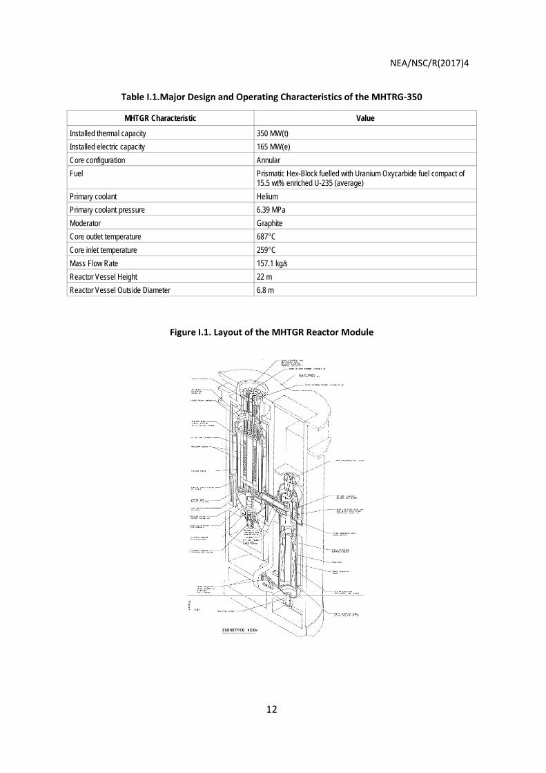
The MHTGR-350 is a General Atomics (GA) design that was developed in the 1980s. The Nuclear Steam Supply (NSS) module arrangement is shown in Figure I.1 and the main characteristics of the design are summarised in Table I.1. The reactor vessel contains the reactor core, reflectors and associated neutron control systems, core support structures, and shut-down cooling heat exchanger and motor-driven circulator. The steam generator vessel houses a helically coiled steam generator bundle as well as the motor-driven main circulator [2]. The pressure-retaining components are constructed of steel and designed using existing technology.

The Reactor Pressure Vessel (RPV) is un-insulated to provide for decay heat removal under loss-of-forced-circulation conditions. In such events, heat is transported to the passive Reactor Cavity Cooling System (RCCS), which circulates outside air by natural circulation within enclosed panels surrounding the RPV. No valves, fans, or other active components or operator actions are needed to remove heat using the RCCS. The reactor core and the surrounding graphite neutron reflectors are supported within a steel reactor vessel. The restraining structures within the reactor vessel are a steel and graphite core support structure at the bottom and a metallic core barrel around the periphery of the side reflectors.

NEA/NSC/R(2017)4

12

Table I.1.Major Design and Operating Characteristics of the MHTRG-350

MHTGR Characteristic Value

Installed thermal capacity 350 MW(t) Installed electric capacity 165 MW(e) Core configuration Annular Fuel Prismatic Hex-Block fuelled with Uranium Oxycarbide fuel compact of

15.5 wt% enriched U-235 (average) Primary coolant Helium Primary coolant pressure 6.39 MPa Moderator Graphite Core outlet temperature 687°C Core inlet temperature 259°C Mass Flow Rate 157.1 kg/s Reactor Vessel Height 22 m Reactor Vessel Outside Diameter 6.8 m

Figure I.1. Layout of the MHTGR Reactor Module

NEA/NSC/R(2017)4

13

I.5.The MHTGR-350 reactor unit specification

This section provides a description of the MHTGR-350 reactor design. The level of detail included is beyond that necessary to perform the benchmark exercises. Nevertheless, due to the variety of modelling techniques, this material is expected to supplement the information supplied in the neutronic and thermal-fluids definitions, Sections I.7and I.8, respectively.

I.5.1.The reference core design description

The core is designed to provide 350 MWt at an average power density of 5.9 MW/m3. A core elevation view is shown in Figure I.2 and a plane view is shown in Figure I.3. The design of the core consists of an array of hexagonal fuel elements in a cylindrical arrangement surrounded by a single ring of identically sized solid graphite replaceable reflector elements, followed by a region of permanent reflector elements all located within a RPV. The permanent reflector elements contain a 10 cm thick borated region at the outer boundary, adjacent to the core barrel. The borated region contains B4C particles of the same design as in the Fixed Burnable Poison (FBP) (see lower half of Table I.5), but dispersed throughout the entire borated region with a volume fraction of 61%.

The active core consists of hexagonal graphite fuel elements containing blind holes for fuel compacts and full-length channels for helium coolant flow. The fuel elements are stacked to form columns (10 fuel elements per column) that rest on support structures. The active core columns form a three-row annulus with columns of hexagonal graphite reflector elements in the inner and outer regions. Thirty reflector columns contain channels for control rods, and twelve columns in the core also contain channels for the reserve shut-down material.

The annular core configuration was selected, along with the average power density of 5.9 MW/ m3, to achieve maximum power rating and still permit passive core heat removal while maintaining the SiC temperature below ~1 600°C during a conduction cool-down event. The active core effective outer diameter of 3.5 m is sized to maintain a minimum reflector thickness of 1 m within the 6.55 m inner diameter reactor vessel. The radial thickness of the active core annulus was specified on the basis of ensuring that the control rod worths of the reflector located rods would meet all shut-down and operating control worth requirements. The choice of reflector control rods was made to ensure that the control rod integrity is maintained during passive decay heat removal events. These radial dimensions also allow for a lateral restraint structure between the reflector and vessel. The height of the core with ten elements in each column is 7.9 m, which allows maximum power rating and axial power stability over the cycle.

The core reactivity is controlled by a combination of Lumped Burnable Poison (LBP), movable poison and a negative temperature coefficient. This fixed poison is in the form of LBP compacts; the movable poison is in the form of metal clad control rods. Should the control rods become inoperable, a backup reserve shut-down control (RSC) is provided in the form of borated pellets that may be released into channels in the active core.

The control rods are fabricated from natural boron in annular graphite compacts with metal cladding for structural support. The control rods are located in the outer ring of the inner reflector and the inner ring of the outer reflector (Figure I.3). These control rods enter the reflector through the top reactor vessel penetrations in which the control rod drives are housed. The 24 control rods located in the outer reflector are the operating control rods, and are used for control during power operation, and for reactor trip. These operating rods can maintain the required 1% ∆ρ shut-down margin indefinitely under hot conditions, or for at least one day under cold

NEA/NSC/R(2017)4

14

conditions. Locating the operating rods in the outer reflector prevents damage during depressurised or pressurised passive heat removal. The six control rods in the inner reflector are the start-up control rods, which are withdrawn before the reactor reaches criticality. With the start-up and operating rods inserted, a 1% ∆ρ shut-down margin can be indefinitely maintained under cold conditions [3].

The RSC consists of borated graphite pellets, housed in hoppers above the core. When the RSC is actuated, these pellets drop into channels in 12 columns of the active core. The RSC is used to institute reactor shut-down if the control rods become inoperable, or if necessary, to provide additional negative reactivity beyond that available in the inserted control rods.

Figure I.2. MHTGR Reactor Unit layout – Axial

NEA/NSC/R(2017)4

15

Figure I.3.MHTGR Reactor Unit Layout – Plane

I.5.1.1.Fuel element design

There are two types of fuel elements, a standard element (Figure I.4), and a reserve shut-down (Figure I.5) element that contains a channel for RSC. The fuel elements are right hexagonal prisms of the same size and shape as the Fort St. Vrain HTGR elements. The fuel element design description is shown in Table I.3.

The fuel and coolant holes are located in parallel through the length of the element. The standard fuel element contains a continuous array of fuel and coolant holes in a regular triangular array of two fuel holes per one coolant hole. The six corner holes contain LBP compacts.

Permanent Reflector (2020

Graphite)

Replaceable Reflector Block (H-451 Graphite)

Replaceable Reflector Block with CR Hole (H-451 Graphite)

Fuel Block with RSC Hole (H-451

Graphite)

Fuel Block (H-451 Graphite)

Core Barrel (Alloy 800H) Coolant Channel RPV (SA-533B)

Neutronic Boundary

Outside Air

NEA/NSC/R(2017)4

16

Table I.2.Core Design Parameters

Core Parameter Value Unit

Thermal Power 350 MW(t)

Core power density 5.93 MW/m3

Number of fuel columns 66

Effective inner diameter of active core 1.65 m

Effective outer diameter of active core 3.5 m

Active core height 7.93 m

Number of fuel elements

Standard elements 540 10/column

RSC elements 120

Number of control rods

Inner reflector 6

Outer reflector 24

Number of RSC channels in core 12

Compacts per core (approximate) 2.0358E+06

Particles per core (approximate) 1.2186E+10

At each element-to-element interface in a column, there are four dowel/socket connections, which provide alignment of coolant channels. A 3.5-cm diameter fuel-handling hole, located at the centre of the element, extends down about one-third of the height, with a ledge where the grapple of a fuel-handling machine engages.

NEA/NSC/R(2017)4

17

Figure I.4. Standard Fuel Element [units in inches]

NEA/NSC/R(2017)4

18

Table I.3.Fuel Element Description

Fuel Element Geometry Value Units

Block graphite density (for lattice calculations) 1.85 g/cm3

Fuel holes per element

Standard element 210

RSC element 186

Fuel hole radius 0.635 cm

Coolant holes per element (large/small)

Standard element 102/6

RSC element 88/7

Large coolant hole radius 0.794 cm

Small coolant hole radius 0.635 cm

Fuel/coolant pitch 1.8796 cm

Block pitch (AF distance) 36 cm

Element length 79.3 cm

Fuel-handling diameter 3.5 cm

Fuel-handling length 26.4 cm

RSC hole diameter 9.525 cm

LBP holes per element 6

LBP radius 0.5715 cm

LBP gap radius 0.635 cm

NEA/NSC/R(2017)4

19

Figure I.5.Reserve Shut-down Control (RSC) Fuel Element [units in inches]

I.5.1.2. Fuel particle and compact design

The fuel is comprised of Tristructural-Isotropic (TRISO) fuel particles bonded in a cylindrical graphite matrix to form a compact. The compacts are then inserted into hexagonal graphite blocks to construct a fuel element. TRISO particles consist of various layers acting in concert to provide a containment structure that limits radioactive product release. They include a fuel kernel, porous carbon layer, inner pyrolitic carbon (IPyC), SiC, and outer pyrolitic carbon (OPyC). The buffer layer allows for limited kernel migration and provides some retention of gas compounds. The silicon carbide layer ensures the structural integrity of the particle under constant pressure and also helps retain metallic fission products. Details of the TRISO particle and compact designs are given Table I.4. These specifications are different from the initial GA design and use a single particle design as requested by the NGNP project.

NEA/NSC/R(2017)4

20

Table I.4. TRISO/Fuel Compact Description

TRISO Fuel Element (general design parameters for lattice calculations) Value Unit

Fissile material UC0.5O1.5

Enrichment (235U average) 15.5 w/o

Radii

Kernel 0.02125 cm

Buffer 0.03125 cm

IPyC 0.03475 cm

SiC 0.03825 cm

OPyC 0.04225 cm

Densities

Kernel 10.5 g/cm3

Buffer 1.0 g/cm3

IPyC 1.9 g/cm3

SiC 3.2 g/cm3

OPyC 1.9 g/cm3

Packing Fraction (average) 0.350

Compact Radius 0.6225 cm

Compact Gap Radius 0.635 cm

Compact Length 4.928 cm

I.5.1.3.Lumped burnable poison design

The LBP consists of boron carbide (B4C) granules dispersed in graphite compacts. The B4C granules are pyrolitic carbon (PyC) coated to limit oxidation and loss from the system. The amount of burnable poison is determined by reactivity control requirements, which may vary with each reload cycle. The diameters of the FBP rods are specified according to requirements for self-shielding of the absorber material to control its burnout rate relative to the fissile fuel burnout rate. The goals are to achieve near complete burnout of the material when the element is replaced, and to minimise the hot excess reactivity swing over the cycle. The current design uses six LBP rods per element in all core layers. Depending on the core design axial zoning is performed through having relatively less LBP mass in the top and bottom layers compared to the middle layers of the core. Axial LBP zoning is used to maintain the axial power shape during burn-up and to prevent xenon induced axial power oscillations. The current design also uses a constant FBP compact diameter of 1.143 cm for all cycles. Details of the FBP design are given in Table I.5.

NEA/NSC/R(2017)4

21

Table I.5.Lumped Burnable Poison Description

LBP holes per element 6

LBP compacts per LBP rod 14

Compact diameter [cm] 1.143

Compact length [cm] 5.156

Rod length [cm] 72.187

Volume fraction of B4C particles 0.109

FBP Component Composition Diameter [µm]

Thickness [µm]

Density [g/cm3]

B4C Particle

Kernel B4C 200 - 2.47

Buffer coating Graphite - 18 1.0

Pyrolitic coating Graphite - 23 1.87

Matrix Graphite - - 0.94

I.5.1.4. Replaceable reflector design

The replaceable reflector elements are graphite blocks of the same shape, size, and material as the fuel elements. The top and bottom reflector elements contain coolant holes to match those in the active core. All reflector elements have dowel connections for alignment (see Figure I.6).

The reflector above the active core is composed of two layers: one layer of full-height elements above a layer of half-height elements, for total reflector height of 1.2 m. The top reflector elements channel coolant flow to the active core and provide for the insertion of reserve shut-down material into the active core. They have the same array of coolant holes as the fuel element and the same holes for the insertion of reactivity control devices.

The reflector below the active core has a total height of 1.6 m. It consists of two layers: one layer of two half-height reflector elements above a layer of two half-height flow distribution and support elements. The bottom two elements provide for the passage of coolant from the active core into the core support area. This is accomplished by directing the coolant channel flow to the outside of the core support pedestal. The channels for the control rods and reserve shut-down material (RSS) stop at the top of the lower reflector so that neither the rods nor the RSS material can exit the core at the bottom. However, small holes are drilled through the reflector below the control rod channels so that adequate cooling is provided for the rods when they are inserted in the core or side reflectors without excessive coolant flow through these channels when the rods are withdrawn from the core.

NEA/NSC/R(2017)4

22

Figure I.6.Hexagonal Reflector Element with CR Hole [units in inches]

The outer side reflector includes one full row and a partial second row of hexagonal reflector columns. The outer row of hexagonal elements is solid, with the exception of the handling holes. Twenty-four of the elements in the inner row of the outer side reflector also have a control rod channel as shown in Figure I.3. The control rod channel has a diameter of 10.2 cm until the bottom reflector assembly and narrows down to 2.5 cm. Crushable graphite matrix at the lower end of each control rod channel will limit the load between the control rod assembly and reflector element in the event that the neutron control assembly support fails. The control rod channel is centred on the flat nearest the active core 9.76 cm from the centre of the reflector element. The distance from the flat of the reflector block to the edge of the control rod channel is 2.7 cm.

The inner (central) reflector includes 19 columns of hexagonal elements. The central and side reflector columns consist of, from top down, one three-quarter-height element, eleven full-height elements, one three-quarter-height element, and two half-height elements, above the core support pedestal. The total reflector height for the equivalent 13.5 elements above the top of the core support pedestal is 10.7 m. The dowel/socket connection at each axial element-to-element interface provides alignment for refuelling and control rod channels, and transfers seismic loads from reflector elements. There are six control blocks in the inner reflector.

I.5.1.5. Control rods and RSC

The control rod design used in the MHTGR is shown in Figure I.7. The neutron absorber material consists of B4C granules uniformly dispersed in a graphite matrix and formed into annular

NEA/NSC/R(2017)4

23

compacts. The boron is enriched to 90 w/o 10B and the compacts contain 40 w/o B4C. The compacts have an inner diameter of 52.8 mm, an outer diameter of 82.6 mm, and are enclosed in Incoloy 800H canisters for structural support. Alternatively, carbon-fiber reinforced carbon (CC) composite canisters, or SiC, may be used for structural support. The control rod consists of a string of 18 canisters with sufficient mechanical flexibility to accommodate any postulated offset between elements, even during a seismic event.

The reserve shut-down control material consists of 40 w/o natural boron in B4C granules dispersed in a graphite matrix and formed into pellets. The B4C granules are coated with PyC to limit oxidation and loss from the system during high-temperature, high moisture events. When released into the RSS channel in the fuel element, the pellets have a packing fraction of ≥ 0.55.

Figure I.7. Control Rod Design

The control rods are withdrawn in groups with three control rods in each group. These three control rods are symmetrically located around the core, so that one rod is located in each 120° sector of the core. During normal power operation, control is accomplished with only the operating control rods (the start-up control rods are in the fully withdrawn position.) These rods are operated automatically on the demand signal from the Plant Control Data Instrumentation System (PCDIS) in symmetric groups. The neutron-flux level is continuously monitored by the ex-vessel detectors that supply signals to the PCDIS, the Investment Protection System (IPS) and the Reactor Protection System (RPS).

NEA/NSC/R(2017)4

24

I.5.1.6.Permanent reflector design

The permanent reflector provides the transition from the hexagonal core to the cylindrical core boundary (Figure I.3). Neutron shielding of the reactor structural equipment consists of graphite permanent reflector elements containing a 10 cm thick borated region at the outer boundary, adjacent to the core barrel. The borated region contains B4C particles of the same design as the LBP. As opposed to containing the particles in compacts, the current design assumes B4C particles are dispersed throughout the entire borated region, and the volume fraction the particles occupy within the borated region is 0.61. This borated region is not modelled in the benchmark; instead the neutronic boundary is placed between the borated region and the core barrel.

I.6. Core layout

I.6.1.Reactor and core structure geometry and dimensions

The benchmark reactor unit geometry definition is given in this section. Figures I.8 and I.9 show the general layout of the reactor. The dimensions of the key components are included in Figures I.10 and 11. The origin for the radial dimension is set at the centre of the core axis. The origin for the axial dimension is set at the bottom of the RPV. The origin for the azimuthal dimension is set at the 120o symmetry line shown in Figure I.8 and moves clockwise. Note that the distance specified below the active core region includes the bottom reflectors and the graphite core support structure.

Figure I.8. Core Radial Layout


Graphite)




Graphite)



Neutronic Boundary

Outside Air

120o Symmetry Line

NEA/NSC/R(2017)4

25

Figure I.9. Core Axial Layout

RPV

Helium Gap

Upper Plenum

Coolant Channel

Metallic Plenum Element (Alloy 800H)

Core Restraint Element (Alloy 800H)

Upper Reflector Block

Fuel Block

Fuel Block with RSC Hole

Replaceable Reflector Block

Replaceable Reflector Block with CR Hole

Core Barrel

Metallic Core Support Structure (MCSS) (Alloy 800H)

Fluid Outlet

Outlet Plenum

Ceramic Tile (Ceraform 1000)

Upper Plenum Thermal Protection Structure (UPTPS) (Alloy 800H)

Neutronic Boundary

Bottom Reflector Block (H-451 Grph)

Bottom Transition Reflector Block (H-451 Grph)

Flow Distribution Block (2020 Grph)

Post Block (2020 Grph)

Insulation (Kaowool)

Repl. Central Reflector Support Block (2020 Grph)

Fluid Inlet

Outside Air

NEA/NSC/R(2017)4

26

Figure I.10.Core Axial Dimensions

13.34

84.76

103.51

193.56

391.81

471.11

1303.74

1343.39

867.60

946.90

1026.20

1105.50

1184.80

550.41

629.70

709.00

788.30

1617.79

1664.29

1732.29

1745.63

38.74

56.52

253.03

292.68

332.33

0.00

340.8 cm

327.5 cm

320.1 cm

304.9 cm

297.3 cm

59.7 cm

67.3 cm

90.0 cm

1358.63

Elevation (cm)

1868.13

463.3 cm

NEA/NSC/R(2017)4

27

Figure I.11.Core Radial Dimensions

NEA/NSC/R(2017)4

28

I.7. Neutronic definition

The neutronic solution of the benchmark problem is only required on a geometrical subset or a smaller part of the reactor. All regions important to the neutronic solution are included but regions far from the core, where flux solutions may be problematic, were excluded. The axial neutronic mesh extends from the top reflector and core restraint element interface (1303.74 cm in Figure I.10) to the graphite core support structure (just above the outlet plenum at 193.56 cm). Radially the inner radius of the core barrel (279.3 cm in Figure I.11) forms the outer boundary. Two separate numbering systems, whole and active core, are organised in layers and columns. Figure I.12 shows the whole-core region numbering for the 1/3

rd core. The bottom reflector is defined as layer 1. Radially the central column is column 1, the rest of the numbering follows the various radial rings up to 91 columns.

Figure I.12. “Whole-Core” Numbering Layout (Layer 1)

NEA/NSC/R(2017)4

29

NOTE: blocks 44 and 51 are part of the permanent reflector region and blocks 22 and 27 are part of the replaceable reflector region. Blocks 74 and 83 are not inside the physical core region, as depicted in Figure I.13. This “whole-core” layout is used to simplify the calculation for participants that do not have the capability to transition from a hexagonal or triangular to a cylindrical geometric description of the permanent reflector region. In addition, some of the distributions provided, e.g., fluence, follow this numbering system.

Figure I.13. Hexagonal and Cylindrical Mesh Superposition

NEA/NSC/R(2017)4

30

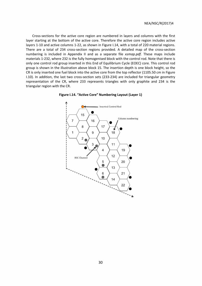
Cross-sections for the active core region are numbered in layers and columns with the first layer starting at the bottom of the active core. Therefore the active core region includes active layers 1-10 and active columns 1-22, as shown in Figure I.14, with a total of 220 material regions. There are a total of 234 cross-section regions provided. A detailed map of the cross-section numbering is included in Appendix II and as a separate file xsmap.pdf. These maps include materials 1-232, where 232 is the fully homogenised block with the control rod. Note that there is only one control rod group inserted in this End of Equilibrium Cycle (EOEC) core. This control rod group is shown in the illustration above block 15. The insertion depth is one block height, so the CR is only inserted one fuel block into the active core from the top reflector (1105.50 cm in Figure I.10). In addition, the last two cross-section sets (233-234) are included for triangular geometry representation of the CR, where 233 represents triangles with only graphite and 234 is the triangular region with the CR.

Figure I.14. “Active Core” Numbering Layout (Layer 1)

NEA/NSC/R(2017)4

31

I.7.1.Neutronic simplifications

The following simplifications are assumed for the neutronic definition:

• The core is 1/3 symmetric as far as the cross-section specification is concerned.

• The cross-sections in RSC block regions take into account the RSC hole region volume correction. No triangular representation is provided for the RSC regions. Therefore, the cross-sections would represent the average fuel cell in the RSC block, which would include 31 fuel holes per sextant. The use of corrected cross-sections via volume weighting to model the RSC blocks with triangular regions is recommended. The weights should be as follows:

• The cross-sections for the control rod regions in the inner and replaceable reflectors

should be volume corrected, if possible. The cross-sections should be multiplied by 0.9278 for a hexagonal representation and by 0.5666 for the triangular representation of the CR region. Not performing a volume correction for those regions is also acceptable since the effect on the neutronic solution is very small.

• Neutron streaming in the gaps, coolant holes, and control holes is ignored.

• Axial dimensions of the fuel rod are simplified: the length of the fuel rods and FBP are assumed to be the full height of the block, the fuel-handling holes are replaced with graphite, and the axial details of the control rods are ignored.

• The borated region by the core barrel is not explicitly modelled. The boundary condition is placed in the inner core barrel where the borated region ends.

• Element bowing due to temperature gradients is ignored.

• All fuel blocks contain FBPs, but for the EOEC core the burnable poison concentration should be small for the once-burned fuel blocks and exhausted for the twice-burned fuel blocks. Consequently, there is no need for special modelling of the FBP region and its homogenisation should yield acceptable results.

I.7.2. Neutronic boundary conditions

The boundary conditions that need to be imposed on the neutronic domain are shown in TableI.16.

13/31

34/31 34/31

35/31 35/31

35/31

NEA/NSC/R(2017)4

32

Table I.6.Neutronic Boundary Conditions

Description Position [cm] B.C. Type 1 Outer boundary (inner radius of

core barrel) 297.30 Non-re-entrant current/Vacuum

2 Below upper core restraint element

1303.74 Non-re-entrant current/ Vacuum

3 Below graphite core support structure

193.56 Non-re-entrant current/ Vacuum

4 Core segment sides (1/3 core segment) Periodic

I.7.3. Description of the cross-section tables

This section outlines the format and origin of the cross-section tables, which are generated for the MHTGR benchmark. The exposure and burn-up history for the equilibrium cycle is taken into account implicitly in the cross-section libraries by defining the different fuel mixtures. The average isotopic composition of the different regions of the core was determined as discussed in Section I.7.3.1.

Two sets of cross-sections are provided. The first set is referred to as the simplified set since the macroscopic cross-sections provided are constant and thus contain no dependence on changing core conditions or state parameters. This set is therefore only useful to test the neutronic solver.

The second set contains cross-sections as a function of a number of state parameters and is therefore used for the actual coupled calculations (see Section I.7.3.3).

I.7.3.1. Number densities used to generate cross-sections

Prismatic block-averaged number densities were generated by GA with the DIFF3D code at EOEC conditions. There are 220 number density sets for the fuel regions. The block-averaged number densities were converted to the corresponding number densities for the DRAGON-4 lattice physics definition including FBPs, compacts, and the various TRISO particle coatings. Reflector and control rod number densities originate from the MHTGR Nuclear Physics Benchmark [4]. The file GA_Number_Densities.csv (distributed to participants) includes the original number densities (in atoms/barn/cm) supplied by GA. The majority of the isotopes are self-explanatory with the following exceptions:

• NSAG25 - non-saturating aggregate fission products from 235U fission;

• NSAG49 - non-saturating aggregate fission products from 239Pu fission;

• 10B – 10B content in the FBP;

• BIMP - burnable impurities in block graphite;

• NBIMP - non-burnable impurities in block graphite;

• OXYGEN – Oxygen content in the fuel compacts;

• C-Fuel - Carbon content in the fuel compacts;

• C-Mod - Carbon content in the fuel block.

NEA/NSC/R(2017)4

33

In order to convert the non-saturating aggregate fission products to an equivalent boron concentration a functionalisation to the 10B concentration in the FBP’s is provided in Table I.7.

To represent the graphite impurities the equivalent 10B atom densities are computed with:

𝑁 𝐵510 =

0.199 ∗ CAWBAW

∗ Nc ∗ NBE ∗ 1𝑥10−6

where,

CAW = carbon atomic weight (12.011)

BAW = natural boron atomic weight (10.811)

Nc = homogenised carbon atom density

NBE = natural boron equivalent total impurity (PPM by weight)

NBE for BIMP = 1.45

NBE for NBIMP = 0.05

For the replaceable and non-replaceable reflector block cross-sections the graphite number density was 8.62465x10-2 atoms/barn-cm and the 10B impurity was 2.76490x10-8 atoms/barn-cm.

Table I.7. Parameters to Determine the Equivalent Boron Concentration for NSAG

Fractional Absorptions NSAG-to-10B

BOEC Fast Thermal Total (Total Ratio) 10B 1.06E-02 8.34E-02 9.39E-02 NSAG25 6.92E-04 7.01E-04 1.39E-03 0.015 NSAG49 4.57E-04 2.33E-04 6.91E-04 0.007

MOEC 10B 5.43E-03 4.91E-02 5.45E-02 NSAG25 1.25E-03 1.27E-03 2.53E-03 0.046 NSAG49 9.44E-04 4.88E-04 1.43E-03 0.026

EOEC 10B 3.01E-03 2.97E-02 3.27E-02 NSAG25 1.62E-03 1.70E-03 3.33E-03 0.102 NSAG49 1.49E-03 7.87E-04 2.27E-03 0.07

I.7.3.2. Simplified macroscopic cross-sections

The purpose of the simplified macroscopic cross-section set is to provide a reference that can be used to test and compare stand-alone neutronic predictions by using the same cross-sections with no thermal-fluids feedback. This will help to understand and quantify the differences introduced by the various neutronics models used and assist in the process to narrow them down. The set is generated from DRAGON-4 lattice physics calculations and based on the DIFF3D EOEC number densities. The cross-sections are homogenised over the block and condensed into 26 energy groups. The tabulation is included in the ASCII file OECD-MHTGR350_Simplified.xs. The computer

NEA/NSC/R(2017)4

34

code xslook, described in Appendix VIII, is provided to load these cross-sections. A description of the simplified cross-section tabulation is included in Appendix II.

I.7.3.3. Four-dimensional cross-section tables

Four-dimensional tables are used to represent the instantaneous variation in cross-section due to changes in the reactor. The cross-section models are designed to cover the initial steady-state conditions and the expected ranges of the four selected instantaneous feedback parameters in the transients to be simulated in the benchmark. The set is generated from the DRAGON-4 code using the end of equilibrium core number densities, homogenised and condensed to 26-energy groups.

Cross-sections are generated for all the combinations of the given state parameters. The four state parameters are:

• fuel temperature (at four values);

• moderator temperature (at seven values);

• 135Xe concentration (at three values);

• hydrogen concentration (at three values).

For the non-fuel materials, no fuel temperature or xenon variations are included. The hydrogen concentrations are only defined for the active core region.

The cross-section file named OECD-MHTGR350.xs is the ASCII data file that will be used for all steady-state and transient exercises that include temperature feedback. The computer code xslookTR, described in Appendix VIII, is provided to load and perform the 4th dimensional linear interpolation of the cross-sections.

I.7.3.3.1. State parameters

The ranges chosen for each parameter were selected based on the reactor conditions for normal operation as well as for accident conditions. The following values for the four state parameters were selected:

• fuel temperature (Doppler temperature): 293 K, 800 K, 1 400 K, 2 000 K;

• moderator temperature: 293 K, 600 K, 800 K, 1 000 K, 1 200 K, 1 600 K, 2 000 K;

• 135Xe concentrations expressed as homogenised concentrations: 0.0, 2.0E-11, 5.0E-10 [#/barn-cm];

• 1H concentration in the steam: 0.0, 3.0E-4, 7.5E-4 of 1H inventory in the core void volumes [#/barn-cm].

No extrapolation will be calculated and any values that go beyond the analysis range will maintain the maximum or minimum values within the analysis envelope.

A description of the cross-section tables is included in Appendix III.

I.7.3.3.2. Additional notes on the OECD-MHTGR350.xs cross-section tables

• All macroscopic cross-sections are specified in units of cm-1.

• The supplied cross-sections are macroscopic, except for Xenon absorption cross-section which is a microscopic cross-section (barns).

NEA/NSC/R(2017)4

35

• The total macroscopic absorption cross-sections provided exclude the absorption effect of xenon. This should be treated explicitly by the participants’ codes. During the cross-section generation process the xenon absorption was subtracted from the macroscopic cross-section using the microscopic cross-sections and the input xenon number densities.

• The 2l+1 factor is not included in the angular moments of the scattering cross-sections and should be treated explicitly:

𝜎𝑠ℎ→𝑔�Ω��⃗ → Ω��⃗ ′� = �

2𝑙 + 14𝜋

𝐿

𝑙=0

𝑃𝑙�Ω��⃗ ∙ Ω��⃗ ′�𝜎𝑙ℎ→𝑔

• The diffusion coefficients should be computed by the participants based on the supplied transport cross-sections. The simplified cross-section set already includes pre-computed diffusion coefficients.

• The β (delayed neutron fraction) values are given per material per energy group.

• κ (energy release per fission) values are given per material in Joules. Note that this value is not dependent on neutron energy, since it has been already integrated in energy within the lattice physics computations.

I.8. Thermal fluids definition

The thermal fluids model of the benchmark is designed to preserve all the characteristics and phenomena related to the heat transfer and fluid flow in the MHTGR-350 design. In order to reduce the complications in the computational modelling of the benchmark core, some minor simplifications were made to the geometry.

In the original MHTGR design, the helium coolant enters the core from the cross-duct, flows down to the bottom of the metallic core support structure (MCSS) and cools down the MCSS via a U-turn before entering the riser/coolant channels. To reduce the complexity of the flow at the entrance, the flow inlet is placed at the bottom of the RPV and oriented along the vertical axis of the reactor. The coolant then flows radially outward to cool down the MCSS via the original flow path.

Another simplification is assumed in the upper plenum region by removing the structure between the core restraint elements and the upper plenum. The helium from the coolant channels flows directly into the upper plenum and is then directed through the fuel blocks.

Several of the materials that constitute the core are sensitive to both temperature and neutron exposure. Neutron exposure has been tabulated in terms of fluence for graphite and burn-up for the kernel thermo-physical properties. Fluence maps are based on the numbering included in Figure I.12. Burn-up maps and the power density map used in steady-state Exercise 2 are based on the numbering included in Figure I.14. Appendix VII includes a description of the input data files provided to perform this benchmark. In addition, a number of FORTRAN computer codes are also provided to load the data from these files into full core (Figure I.12) arrays. A discussion of the various computer codes provided to load the power density, burn-up, and fluence maps are included in Appendix VIII.

Note that the stagnant helium outside the flow channels between the core barrel and RPV is assumed to be at reactor pressure.

NEA/NSC/R(2017)4

36

I.8.1.Thermal fluids simplifications

The following simplifications are assumed for the thermal fluids definition:

• The cross-duct has been oriented in the axial direction to simplify the modelling.

• The RSC and handling holes in fuel regions are not considered flow regions; they contain stagnant helium at reactor pressure.

• The control rod holes are considered part of the by-pass flow in CR regions. The bottom sections of the CR holes are engineered to limit the flow through them. The specifications are included in Table I.9.

• The effect of excluding specific coolant flows is to some extend balanced by the assumption that all heat sources (from fission) will be deposited locally, i.e. in the fuel and that no other heat sources exist outside the core (for example neutron absorption in the control rods). Simplifications are also made in the material thermal properties in as far as constant values are employed or specific correlations are employed. These assumptions are clearly listed in the sections that follow.

• No cross flow in the by-pass gaps or below the fuel blocks is modelled.

• The RCCS is not explicitly modelled, but radiation heat transfer from the RPV to the ultimate heat sink (RCCS) through the outside air (assumed stagnant) should be modelled with an RCCS emissivity assumed to be 0.80. In order to simplify the modelling an effective emissivity of 0.74 should be used to represent the RPV and the air between the RPV and RCCS.

• Assume that the radial conductivity of the block is well approximated with the thermal unit cell described in Appendix IV-4. The centre and peripheral graphite regions within the block are ignored.

• The thermo-physical properties should be adjusted for porosity changes, if applicable, with the exception of exercises where fixed thermo-physical properties are provided.

• Roughness factors for the flow channels are assumed to be 0.

• Assume full height fuel and LBP.

• The original MHTGR-350 graphite material H-451 was replaced by PCEA AG from another vendor, according to information verified with GA. The density of PCEA AG (1 850 kg/m3) has therefore been used for both the neutronic and thermal fluid specification, but since no information are available on the behaviour of PCEA AG under exposure to fluence, the thermal conductivity and specific heat capacity of H-451 graphite (sourced from the Graphite Handbook) were assumed to apply to PCEA AG for the purposes of this benchmark.

I.8.2. Reactor thermal fluids layout

The radial and axial layouts of the core are shown in Figure I.8 and Figure I.9 .The radial geometry for the thermal fluids model extends to the stagnant air volume outside the RPV. The geometry in the axial direction extends to the air layer outside the top surface of the RPV.

NEA/NSC/R(2017)4

37

I.8.3. Reactor main coolant flow specifications

The main flow specifications are included in Table I.8. For this simplified model the cross-duct is oriented in the axial direction at the bottom of the RPV. The helium coolant enters the core from the outer shell of the hot duct, cools down the bottom plate and flows up in the 12 riser/coolant channels located between the core barrel and RPV. When it reaches the upper plenum, it is directed down through the core coolant channels and by-pass flow spaces. The coolant channels extend from the top of the core to the bottom reflector block. The flow then continues through the bottom transition reflector block and the flow distribution block before reaching the post block and the outlet plenum. The coolant exits the reactor through the inner shell of the hot duct. Table I.9 includes the flow parameters that should be used in the modelling of the flow path. All RSC and fuel-handling holes are not considered flow regions and they contain stagnant helium. The fuel holes are not flow regions and the top reflector blocks do not contain coolant holes that match the fuel holes. The main coolant flow map is shown in Figure I.15. Participants that cannot model the coolant channels explicitly should assume that the flow is equally distributed azimuthally.

Figure I.15. Main Core Flow Path

RPV

Helium Gap

Upper Plenum

Coolant Channel




Fuel Block




Core Barrel


Fluid Outlet

Outlet Plenum









Fluid Inlet

Outside Air

NEA/NSC/R(2017)4

38

Table I.8. Main Flow Specifications

# Description Unit Value

1 He inlet temperature ºC 259.0 2 He outlet temperature ºC ~687.0 3 Total inlet mass flow rate kg/s 157.1 4 Outlet pressure MPa 6.39

Table I.9. Flow Parameters

# Description Unit Value

Hot duct inside radius cm 59.7 Hot duct outer radius cm 67.3 Thermal barrier (between inlet and outlet ducts) thickness cm 7.62 Cross-duct inside radius cm 90.0 Coolant channel depth (between core barrel and RPV) cm 15.24 Coolant channel length cm 66.04 Coolant channel thickness (assumed) cm 2.54 Standard fuel block porosity 0.186 RSC block porosity (RSC hole is not a flow region) 0.165 Bottom reflector block height cm 59.47 Bottom reflector block porosity (STD/RSC) 0.199/0.177 Flow transition block height cm 39.65 Flow distribution block height cm 39.65 Post block height cm 59.47 Outlet plenum porosity 0.6 CR channel radius (from axial position 193.56 cm to 391.81 cm) cm 1.25 CR channel radius (from axial position 391.81 cm to 1343.39 cm) cm 5.08

I.8.4. Boundary conditions

The top and side boundaries are at a fixed temperature, representing the RCCS, located 122.5 cm from the outer surface of the RPV. The bottom boundary condition is adiabatic at the RPV outer surface. The properties of stagnant air must be used if conduction and convection are modelled in the region between the RPV and the RCCS. The thermal fluids boundary condition specifications are shown in Table I.10.

NEA/NSC/R(2017)4

39

Table I.10. Thermal Fluids Boundary Conditions

Thermal Fluids Model Boundaries (cm) 1 Radial (outside air boundary) 463.30 2 Top (outside air boundary) 1868.13 3 Bottom 0 Thermal Fluids Boundary Conditions 1 Radial Constant Temperature 30 oC 2 Top Constant Temperature 30 oC 3 Bottom Adiabatic 4 Radial and Top The ultimate heat sink (RCCS) emissivity is 0.8. Alternatively,

the effective emissivity of the RPV and air can be assumed to be 0.74.

I.8.5. By-pass flow specification

The by-pass flows considered in this benchmark are divided into four categories. These include engineered and unintended by-pass flows, and occur in in-core gaps, ex-core gaps, reflector coolant channels and control rod channels. Figure I.16 shows the by-pass flow paths.

The by-pass gaps for the fuel and replaceable reflector blocks are assumed to affect only the thermal fluids characteristics of the core via a reduction in conduction heat transfer, and increases in convective and radiation heat transfer. The size of the block will remain at 36 cm across the flats.

NEA/NSC/R(2017)4

40

Figure I.16. Core By-pass Flow Paths

RPV

Helium Gap

Upper Plenum

Coolant Channel




Fuel Block




Core Barrel


Fluid Outlet

Outlet Plenum









Fluid Inlet

Outside Air

NEA/NSC/R(2017)4

41

I.8.5.1. Type-I

This first type of by-pass flow is specified in Table I.11 and azimuthally uniform for each radial ring of the core. This introduces a more complex spatial dependency on the by-pass flow distribution.

Table I.11. By-pass Flow Distribution

Component % of Total Flow 1 In-core 1.50 2 Inner Reflector 0.50 3 Inner Control Rod Cooling 1.20 4 Outer Control Rod Cooling 1.80 5 Outer Reflector (First Ring) 1.38 6 Outer Reflector (Second Ring) 1.62 7 Permanent Side Reflector 3.00 Total 11.00

I.8.5.2.Type-II

The by-pass region is modelled explicitly and the by-pass flow is a calculated parameter. Participants will be asked to describe their approach to modelling the by-pass. The by-pass flow gap sizes are given in Table I.12.

Table I.12.By-pass Flow Gap Sizes

Flow Path Width (mm) 1 Gaps between blocks (fuel or replaceable reflector) 2.0 2 Gaps between Permanent Side Reflector and Core Barrel 3.5 3 CR channel radius (from axial position 193.56 cm to 391.81 cm) 12.5 4 CR channel radius (from axial position 391.81 cm to 1343.39 cm) 50.8

I.8.6. Fuel temperature model

An accurate fuel model is necessary in order to simulate the MHTGR reactor since the fuel temperature feedback dominates its neutronic behaviour. Schematics of the fuel unit cell for the MHTGR block are shown in Figures I.17 and I.18. Note that there is a 0.1 mm gap between the fuel compact and the graphite, filled with stagnant helium.

NEA/NSC/R(2017)4

42

Figure I.17. Fuel Unit Cell - Block Geometry

Figure I.18. Fuel Unit Cell – Detailed (note 0.1 mm gap)

I.8.7. Material properties

The participants must calculate the effective block conductivities based on the data provided. The conductivity of the fuel blocks is a tensor with radial and axial components. The radial effective conductivity of the fuel compact and the thermal unit cell should be determined from the AMEC model [5]. This AMEC model and the axial conductivity equation for the thermal unit cell are described in Appendix IV.

NEA/NSC/R(2017)4

43

Temperature and fluence dependent thermo-physical properties are provided where relevant. The file OECD-MHTGR350-fluence.inp includes the fluence distribution in all regions of the core including reflector regions. The file OECD-MHTGR350-burn-up.inp includes the burn-up distribution in the active core regions. FORTRAN-90 subroutines are provided to load all burn-up and fluence distributions and to calculate the various thermo-physical properties, to ensure consistency between participants.

I.8.8. Decay heat

For the benchmark problem the decay heat source is only of importance in certain transient cases, typically where the fission power is reduced to zero during the event. For the steady-state cases the decay heat is assumed to be part of the energy released per fission, which are assumed in this specification to be all deposited locally, i.e. where the fission took place. Therefore, the total core power = fission power + decay heat power = 350 MW. During the Depressurised and Pressurised Conduction Cooldown (DCC/PCC) transients (Volume IV, Exercises 1 and 2) the time dependent decay heat calculation should start as soon as the transient starts (t=0 sec) and the fission power starts decreasing.

The decay heat value for each material mesh, as calculated for the EOEC, is shown in Appendix I. It was derived making use of the relative core average decay heat behaviour (values provided as determined from the DIN 25485 standard [11]) and the material mesh power. This implies that the decay heat is directly related to the steady-state power produced in the mesh prior to the start of the transient. No history effects or power excursions after the start of the transient should be taken into account (e.g., see Volume IV, Exercises 3 and 4), and participants should not use their own decay heat data.

NEA/NSC/R(2017)4

44

Volume II. Definition of the Steady-State Exercise

NEA/NSC/R(2017)4

45

II.1. Steady-state benchmark calculational cases

General note on reporting of data:

A code-dependent, spatially converged calculation mesh must be determined by each participant, but the spatial mesh format prescribed in the output data Section II.2 must be used to report data. This might require post-processing of more detailed participant data to volume-averaged comparison values.

II.1.1. Case definitions

II.1.1.1. Exercise 1: Neutronics solution with fixed cross-sections

The purpose of this first exercise is to ensure that there are no significant differences in the neutronics models between participants that would affect subsequent exercises. Make use of the model description, data reporting template in Figure II.9 and the following conditions to obtain a neutronics-only solution:

• Use the provided simplified cross-section set with no state parameter dependence (Appendix II), and the control rod location specified in Volume I, Section I-7. For this exercise of the benchmark assume that the power generated is 200 MeV per fission event.

• For the triangular representation it is recommended for the cross-sections to be appropriately weighted in the RSC blocks. The weighting is described in Volume I, Section I-7.1.

• For both hexagonal and triangular representation it is recommended for the cross-sections to be appropriately weighted in the control rod blocks. The weighting is described in Volume I, Section I-7.1.

II.1.1.2. Exercise 2: Thermal fluids solution with given power/heat sources

The purpose of this second exercise is to ensure that there are no significant differences in the thermal fluid models between participants that would affect subsequent exercises. Make use of the model description, thermal fluid and material properties (Volume I, Section I-8), the data reporting template in Figure II.10 and the following conditions to obtain a thermal fluids-only solution:

• Use the provided power/heat source density data set, in OECD-MHGTR350-power.inp, a list of files is provided in Appendix VII.

• Four sub cases are defined for Exercise 2:

– Exercise 2a: no modelling of core by-pass flow. Use the fixed thermo-physical properties in Appendix IV, Section IV. All gaps are closed, and no porosity correction should be performed.

– Exercise 2b: use the Type I core by-pass flow distribution specified in Volume I, Section-8.5.1 and the fixed thermo-physical properties in Appendix IV, Section IV-1.

– Exercise 2c: use the Type I core by-pass flow distribution specified in Volume I, Section-8.5.1 and variable thermo-physical properties in Appendix IV.

– Exercise 2d: use the Type II core by-pass flow distribution specified in Volume I, Section-8.5.2 and variable thermo-physical properties in Appendix IV.

NEA/NSC/R(2017)4

46

All participants should complete Exercise 2a through 2c as a minimum requirement. Participants should submit results for all four cases, if the analysis for case 2d is within their code’s capabilities.

II.1.1.3. Exercise 3: Coupled neutronics – Thermal fluids steady-state solution

The purpose of this third exercise is to ensure that the coupling is consistent between participants. Make use of the model description, neutronics (Volume-I, Section I-7), thermal fluid (Volume-I, Section I-8) and material properties (Volume-I, Section I-8.6), the data reporting template in Figure II.11 and the following conditions to obtain a converged Coupled Neutronics and thermal fluids solution:

• Use the provided state parameter dependent cross-section set (Volume-I, Section I-7.3.3) and the control rod location specified in Volume-I, Section I-7.

• For the triangular representation it is recommended for the cross-sections to be appropriately weighted in the RSC and control rod blocks. The weighting is described in Volume I, Section I-7.1.

• For both hexagonal and triangular representation it is recommended for the cross-sections to be appropriately weighted in the control rod blocks. The weighting is described in Volume I, Section I-7.1.

• In steady state, the fuel temperature used for Doppler feedback should be based on a 1/6th block-averaged compact temperature.

• Use variable thermo-physical properties.

• Two sub cases are defined for Exercise 3:

– Exercise 3a: use the Type I core by-pass flow distribution specified in Volume-I, Section I-8.5.1.

– Exercise 3b: use the Type II core by-pass flow distribution specified in Volume-I, Section I-8.5.2, if code capabilities allow.

II.1.2. Convergence criteria

General convergence criteria guidelines are provided in Table II.1. Each participant should ensure that a well-converged result is obtained by performing a sensitivity study on the code-specific input parameters, mesh sizes and acceleration parameters.

Table II.1. Suggested Convergence Criteria

Parameter Unit Convergence criteria keff 1.0E-6 Local Fluxes 1.0E-4 Local Temperatures °C 0.1 Local Flows kg/s 0.1

II.2. Requested output

All output data files should use the XML format delineated in this section. The files should adhere to the UTF-8 (UCS Transformation Format) encoding standard. Any files submitted will be verified

NEA/NSC/R(2017)4

47

for the appropriate format before being accepted for analysis. Sample files as well as a computer code to generate the XML will be provided. The results submitted should be included with the folder structure shown in Figure II.1. The structure will be checked to make sure that it meets the desired organisation.

Figure II.1. Schematic of the Steady-State Results Folder Structure

Note: Any data point for which data is unavailable should be reported as -999.

II.2.1. Reporting requirements

II.2.1.1. Reporting mesh: Neutronics

Even though the calculation mesh can be refined to achieve the desired spatial convergence, the reporting mesh will be performed at the hexagonal block level. Furthermore, if available, researchers can, in addition to block-wise results, submit results at the triangle level as depicted in Figure II.2.

Figure II.2. Triangle Based Reporting

The power density and xenon concentration maps will be reported over the active core region only. The neutronic radial mesh should be either at block or triangular level based on the

Steady-State Exercises

Exercise 1

Exercise 2a

Exercise 3a

Exercise 2b

Exercise 2c

Exercise 3b

Exercise 2d

1 2

4 5

6

3

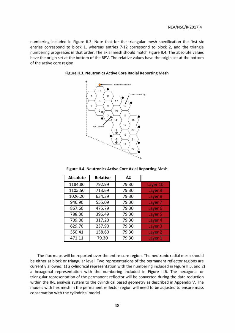
NEA/NSC/R(2017)4

48

numbering included in Figure II.3. Note that for the triangular mesh specification the first six entries correspond to block 1, whereas entries 7-12 correspond to block 2, and the triangle numbering progresses in that order. The axial mesh should match Figure II.4. The absolute values have the origin set at the bottom of the RPV. The relative values have the origin set at the bottom of the active core region.

Figure II.3. Neutronics Active Core Radial Reporting Mesh

Figure II.4. Neutronics Active Core Axial Reporting Mesh

The flux maps will be reported over the entire core region. The neutronic radial mesh should be either at block or triangular level. Two representations of the permanent reflector regions are currently allowed: 1) a cylindrical representation with the numbering included in Figure II.5, and 2) a hexagonal representation with the numbering included in Figure II.6. The hexagonal or triangular representation of the permanent reflector will be converted during the data reduction within the INL analysis system to the cylindrical based geometry as described in Appendix V. The models with hex mesh in the permanent reflector region will need to be adjusted to ensure mass conservation with the cylindrical model.

NEA/NSC/R(2017)4

49

The reporting axial mesh for whole-core flux distributions should conform to that shown in Figure II.7. The absolute values have the origin set at the bottom of the RPV. The relative values have the origin set below the bottom reflector region.

Figure II.5. Neutronics Whole-Core Radial Reporting Mesh for a Cylindrical Permanent Reflector


Graphite)




Graphite)



Outside Air

120o Symmetry Line

1

2

4

8

3 7

13 21

31

57

5

6

12 20

56

9 10

11 19

29 41

55

14 15 16

17 18

28 40

54

22 23

24 25

26 27

39 53

32 33

34 35

36 37

38 52

45 46

47 48

49 50

2

4

8 14

32

3 5

9 15

23 33

45

7 6

10 16

24 34

46

13 12

11 17

25 35

47

21 20

19 18

26 36

48

31 30

29 28

27 37

49

43 42

41 40

39 38

50

57 56

55 54

53 52

3 5

9 15

23

45

7 6

10 16

24

46

13 12

11 17

25

47 35

21 20

19 18

26

48 36

31 30

29 28

27

49 37

43 42

41 40

39

50 38

57 56

55 54

53 52

2 4

8 14

22 32

51

44

58 59

60 61

62 63

64

65

66

67

68

69

70

71

30 42

43 22

34

33

NEA/NSC/R(2017)4

50

Figure II.6. Neutronics Whole-Core Radial Reporting Mesh for a Hexagonal Permanent Reflector

NEA/NSC/R(2017)4

51

Figure II.7. Neutronics Whole-Core Axial Reporting Mesh

II.2.1.2. Reporting mesh: Thermal fluids

Solid and fluid distributions of the results will be reported on the whole-core axial reporting mesh included in Figure II.7. Note that the lower and upper structures including the ceramic tile, MCSS CRE, Plenums, UPTPS, and RPV are not included. Only the maximum MCSS temperatures are reported in the global parameters file. Note that fuel temperatures should only be reported for the active core regions with the reporting mesh included in Figures II.3 and II.4. The fluid temperatures are reported in the same active core regions (1-22) for the thermal-fluid axial layers 1-14 and in the stagnant helium region.

The radial mesh for axial layers 1-14 is shown in Figure II.8. The azimuthal sectors are used to represent regions 58 to 71 in the permanent reflector, regions 72 to 85 in the core barrel, and 86 to 99 in the RPV. The models with hex mesh in the permanent reflector region will need to be adjusted to ensure mass conservation with the cylindrical model. In addition, the modeller needs to take care of the fact that the core barrel is specified for a cylindrical configuration and the reporting is expected as shown in Figure II-8.

By-pass fluid mass flow rates will be reported on the regions defined in Volume I, Table I.11 for axial regions 1.14. Therefore, only seven values are expected per axial region.

Finally, the heat flux normal to the outer surface of the RPV (facing the ultimate heat sink) is reported at the various axial and azimuthal regions for the RPV in axial layers 1.14.

The fluid heat transfer coefficient (Havg) and engineered mass flow rate (Mdot-eng) should be reported in axial layers 1.14.

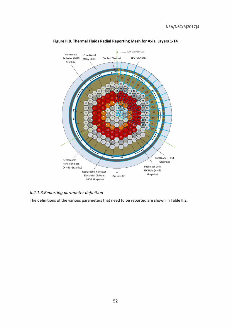
NEA/NSC/R(2017)4

52

Figure II.8. Thermal Fluids Radial Reporting Mesh for Axial Layers 1-14

II.2.1.3.Reporting parameter definition

The definitions of the various parameters that need to be reported are shown in Table II.2.


Graphite)




Graphite)



Outside Air

120o Symmetry Line

1

2

4

8

3 7

13 21

31

57

5 6

12 20

56

9 10

11 19

29 41

55

14 15 16

17 18

28 40

54

22 23

24 25

26 27

39 53

32 33

34 35

36 37

38 52

45 46

47 48

49 50

2 4 8

14

32

3 5

9 15

23 33

45

7 6 10

16 24

34 46

13 12

11 17

25 35

47

21 20

19 18

26 36

48

31 30

29 28

27 37

49

43 42

41 40

39 38

50

57 56

55 54

53 52

3 5

9 15

23

45

7 6

10 16

24

46

13 12

11 17

25

47 35

21 20

19 18

26

48 36

31 30

29 28

27

49 37

43 42

41 40

39

50 38

57 56

55 54

53 52

2 4

8 14

22 32

51

44

58 59 60

61 62

63

64 65

66

67

68

69

70

71

72 73 74 75

76

77

78

79

80

81

82

83

84

85

86 87 88 89

90

91

92

93

94

95

96

97

98

99

30 42

22 43

34

33

NEA/NSC/R(2017)4

53

Table II.2. Output Parameter Definition

Parameter Description Unit

Axial (power) offset AO = (TPtop – TPbottom)/(TPtop + TPbottom), where TPtop = total power produced in the top half of the core, and TPbottom = total power produced in the bottom half of the core.

None

Control rod worth The control rod worth will be calculated for the only inserted bank in the EOEC configuration at full power by performing two eigenvalue calculations. One with the bank at position 391.81 and the other with the bank at position 1184.8 cm.

Δ𝜌𝐶𝑅 =𝑘𝑜𝑢𝑡 − 𝑘𝑖𝑛𝑘𝑜𝑢𝑡𝑘𝑖𝑛

where, kout= eigenvalue with CR at position 1184.8 cm kin= eigenvalue with CR at position 391.81 cm.

pcm

Fuel temperature (average) The “average fuel temperature” T_fuel_avg (in Table II-6) is defined as the average volumetric fuel compact temperature in a single 1/6 block region within a single fuel block (i.e. extending over a height of 79.3 cm, if axial refinements are performed). The volumetric averaging should take the porosity of the regions into account. The global parameter T_fuel_avg_core (in Table II-4) is the volumetric average of the fuel compact temperatures of all these triangular regions in the entire active core region.

oC

Heat flux (RPV) The heat flux normal to the outer RPV surface facing the ultimate heat sink. This heat flux should combine the various heat transfer mechanism being modelled, and is the sum of the upper, radial, and lower RPV contributions. Note that the heat flux should be negative as long as energy is flowing away from the core.

W/m2

Fluid temperature (average) This variable is split into two types: engineered and by-pass flows. The engineered fluid parameters Tfluid-avg-core and Tfluid-max-core should be reported in axial layers 1-14, and is only defined in the active core region. For the volumetric fluid average temperatures the porosity of the regions must be taken into account. By-pass fluid temperatures must be reported on the regions defined in Volume I, Table 11, for axial regions 1-14 (only seven values), and is excluded from the variable Tfluid-avg-core.

oC

Mass flow rate (helium) Mass flow rate of helium coolant in the system Engineered – for all bored channels that flow through the active core By-pass – in gaps between blocks, CR holes.

kg/s

Moderator temperature (average)

The “average moderator temperature” is defined as the average volumetric block graphite temperature in a fuel block. The volumetric averaging should take the porosity of the regions into account.

oC

Fuel temperature (maximum) The “maximum fuel temperature” T_fuel_max (in Table II-6) is defined as the maximum fuel compact temperature in a single 1/6 region within a single fuel block (i.e. extending over an height of 79.3 cm, if axial refinements are performed). The global parameter T_fuel_max_core (in Table II-4) is the maximum value of all fuel compact temperatures in all triangular regions in the entire active core region. For participants that include explicit modelling of the TRISO particles within the fuel compacts, the average and maximum definitions above should be determined as follows: T_fuel_avg (Table II-6): volumetric average of all TRISO layers and all TRISO particles temperatures for all the compacts in a single 1/6 region within a single fuel block (i.e. extending over a height of 79.3 cm, if axial refinements are performed). T_fuel_avg_core (Table II-4): volumetric average of all TRISO temperatures and all 1/6 block regions in the entire active core region. T_fuel_max: maximum of all UC0.5O1.5 kernel temperatures for all the compacts in a single triangular region within a single fuel block (i.e. extending over a height of 79.3 cm, if axial refinements are performed).

oC

NEA/NSC/R(2017)4

54

Parameter Description Unit T_fuel_max_core: maximum of all UC0.5O1.5 kernel temperatures for all the compacts in all 1/6 block regions in the entire active core region. Note: participants should indicate which model was used during data submission to ensure that differences between compact and TRISO based models can be tracked.

Outlet helium temperature Average helium temperature in the outlet duct. oC Power density (average) The average power density is the average homogenised value within the 1/6 single

block reporting region. MW/m3

Power (Total) Total thermal power (i.e. fission power + decay heat). MW Pressure Gage pressure (engineered + by-pass channels). Mpa

Reactivity Global reactivity change, as caused by transient feedback effects (differential change between core states).

pcm

Pressure drop (core) Drop in helium pressure over the core (plenum to plenum). kPa

Reflector temperature (average)

The “average reflector temperature” is defined as the volumetric average temperature in the inner, top, bottom and outer reflector regions. The axial height of the reflector is defined between 292.61 (layer 1) and 1303.74 cm (layer 14). It includes both the replaceable and non-replaceable reflector regions. The volumetric averaging should take the porosity of the regions into account. Note that the graphite in the active fuel core region is excluded, since this is moderator graphite.

oC

Solid temperature Distribution of the solid material temperatures in the reactor. It includes moderator, reflector, core barrel, and RPV. The average solid temperature is the average volumetric value in the reporting region (1/6 block). The volumetric averaging should take the porosity of the regions into account.

oC

Xenon concentration Xenon concentration that occurs in each of the spatial meshes. Since the units for this parameter varies in the different codes, relative xenon values normalised to the steady-state Xenon concentration levels in each of the spatial meshes will be used.

None (normalised to steady-state)

II.2.1.4. Reporting file structure

The files submitted by each participant will be required to meet certain requirements for processing. Each exercise folder should contain two general-purpose files: one named SolutionInfo.xml, and the other named GlobalParam.xml. Note that the names of these two files are important for loading the data in the database. The first file contains researcher and code information and includes a header element with the metadata shown in Table II.3. The second file contains a number of integral and specific local values, shown in Table II.4. These can be time dependent and should include as many entries as specified in the “Num-data-block” parameter included in the same file. All of the values in the GlobalParam.xml file are expected to be computed from the fine, converged mesh used in the simulation. Note: The xml tags are not case sensitive, since the data reader converts all of the XML tags to lower case when loading the data.

Table II.3. Metadata for the Solution Information File

Sub-element name Data type Definition Contact string Contact person Institution string Name of the research institution (use acronym since this field is

used in plotting routines) Country string Country represented

NEA/NSC/R(2017)4

55

Sub-element name Data type Definition Time-stamp

Attributes: Date, Time date and time Date and time when the calculation was completed

Date YYYY-MM-DD Time hh:mm:ss

PHASE Integer 1

Exercise String (1a, 2a, 2b …)

Computer-code String Name of the computer code (use acronym since this field is used in plotting routines)

Computer-code-description Please provide a detailed description of the code system Kconvg Float Keff convergence Fconvg Float Flux convergence Tconvg Float Temperature convergence Method String Finite Difference, Finite Element, Finite volume, etc. Model String Define the equation set used in the problem. For Exercises 2 and

3 describe how the type II by-pass is modelled. Coupling String Type of neutronic-thermal fluids coupling

LC = loosely coupled (operator splitting with forward marching without iterative scheme to converge each solver for each time step) TC = tightly coupled (operator splitting with iterative scheme to converge each solver for each time step) SC = strongly coupled (no operator split) NA = Not Applicable

Table II.4. Metadata for the Global Parameters File

Sub-element name (all floats) Units Definition Time-stamp Attributes: Date, Time

date and time Date and time when the calculation was completed Date YYYY-MM-DD Time hh:mm:ss

Num-data-block integer Number of time dependent data blocks in file Keff unitless Fundamental mode eigenvalue Keff-err unitless Relative error in eigenvalue (if available) CR-worth pcm Control rod worth AO unitless Axial offset (see Table II) Total-power MW Fission + decay power Pden-avg-core MW/m3 Core average power density (see Table II) Tfuel-max-core oC Core maximum fuel temperature (see Table II) Tfuel-avg-core oC Core average fuel temperature (see Table II) Tmod-avg-core oC Core average moderator temperature (see Table II) Trefl-avg-core oC Core average reflector temperature (see Table II) Tfluid-avg-core oC Core average fluid temperature (see Table II) Tbarrel-max oC Core barrel maximum temperature (includes all upper, radial

and lower head structures) TRPV-max oC RPV maximum temperature (includes all upper, radial and

NEA/NSC/R(2017)4

56

Sub-element name (all floats) Units Definition lower head structures)

TMCSS-max oC MCSS maximum temperature Toutlet-avg oC Average fluid temperature at the outlet DP-core kPa Core Pressure Drop (see Table II) Heat-loss-boundary MW Heat loss from the RPV to the boundary (sum of all radial &

axial boundary components)

All data files that include core distributions will contain a header and a body section. Each data file includes only one specific dependent variable distribution: flux, average power, maximum power, etc. The name of these files does not matter as long as they use the .xml extension.

The header section of the core distribution file contains the “File-ID” element, which describes the type and format of the data contained in the file. The “File-ID” element is shown in Table II.5. All files should contain a time stamp. The “Format-type” sub-element sets the flag for reading either block-wise or triangular based distribution in the active core and replaceable reflector regions. The “PR-type” sub-element sets the flag for reading the permanent reflector region as described in Section II.2.2.1. The “Data-name” sub-element of the “File-ID” element includes the dependent variable description and is shown in Table II.5.

Table II.5. “File-ID” Element Description

Sub-element name Data type Definition Time-stamp Attributes: Date, Time

date and time Date and time when the calculation was completed Date YYYY-MM-DD Time hh:mm:ss

Format-type string Hexagon | Triangle PR-type string Hexagon|Triangle|Cylinder (this is the representation of the

permanent reflector region) Num-Data-block integer number of time dependent data blocks in file Data-name string type of data included (see Table II.6)

The body section contains the “Data-body” element, which includes the actual data values

reported on the mesh described in Sections II.2.1.1 and II.2.1.2.

Table II.6. Data-name values for core distributions

Data-name (all floats) Units Description Radial mesh figure

Axial mesh figure

Neutron-flux n/cm2-sec Neutron flux II-5 or II-6 II-7 Xe-con at/barn-cm Xenon concentration II-3 II-4 Pden-avg MW/m3 Power average density II-3 II-4

Pden-avg-err MW/m3 Relative error in the power average density (if available) II-3 II-4

Tfuel-avg oC Fuel average temperatures II-3 II-7

NEA/NSC/R(2017)4

57

Tfuel-max oC Fuel maximum temperatures II-3 II-7

Tsolid-avg oC Average solid temperatures: moderator, reflector,

core barrel, RPV II-8 II-7

Tfluid-avg oC Fluid average temperatures II-3 II-4 Eff-k-radial W/m-K Radial component of conductivity II-8 II-7 Eff-k-axial W/m-K Axial component of conductivity II-8 II-7 H-avg W/m2-K Heat transfer coefficient II-3 II-4 Mdot-eng kg/sec Engineered mass flow rate II-3 II-4 Mdot-by-pass kg/sec By-pass mass flow rate Vol. I, Table 11 II-4 Q-flux-bdy W/m2 Heat flux at RPV II-8 II-7

1RPV values in axial layers 1-18 are reported for regions 28-35.

The “Data-body” element, shown in Table II.7, contains only one type of sub-element, “Data-block,” which marks the beginning of a full distribution of data for one time step. The “Data-block” element has two attributes: one “ID” and a “time” attribute. The first attribute marks the data-block number, the later includes the simulation time in seconds. Within the “Data-block” there are two additional sub-elements. The “Axial-layer” sets the beginning of an axial layer and “Group” sets the beginning of an energy group for flux distributions in that axial layer.

Table II.7. “Data-body” Element Description

Data-body sub-element name Data type Definition/Units Data-block Attributes: ID, Time

ID – integer Time – float

Sets beginning and end of data block

Simulation time is in seconds

Sub-elements: Axial-layer (Attributes: ID)

–D - integer Layer number based on the mesh definition

Group (Attributes: g)–g - integer

Energy group number (flux only)

II.2.1.5. Steady-state output parameters

The files that are requested for the steady-state exercises are listed in Figure II-9 through Figure II.11. Each numbered bullet in the box to the left indicates a separate file with either relevant case information or the appropriate distribution. The box to the right shows the data to be reported in the global parameters file.

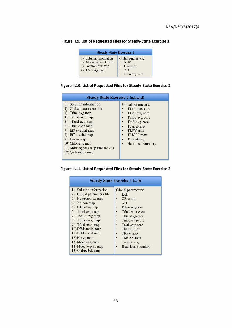
NEA/NSC/R(2017)4

58

Figure II.9. List of Requested Files for Steady-State Exercise 1



NEA/NSC/R(2017)4

59

Appendices

Appendix I. Decay heat calculation

The decay heat calculations for this benchmark are based on the DIN 25485 standard [11]. This standard was developed for HTRs using pebble type fuel, but since the standard only requires accurate spatial power histories, it can be applied to HTRs with prismatic fuel as a good first approximation as well. The evaluation accounts for the contribution of fission products, heavy metals, and isotopes generated by neutron capture of fission products.

The evaluation includes the local generation of decay heat power as a function of the thermal power history of the fuel located at the considered position as a function of the time elapsed after reactor shut-down or the fuel was discharged. The activation of structural material is not accounted for.

The accuracy of the calculation depends on the detail applied to the definition of the power histogram. The power histogram defines the irradiation history of the fuel elements. It divides the operation period of the fuel into time periods, which can be assumed to have constant power, constant sharing of total power between the different fissile isotopes, as well as a constant neutron capture rate of the fertile materials. If the sharing of the power between the different fissile isotopes is not known to the user, the total power may be assigned to 235U.

The power histogram contains the following data:

• length of the small time steps;

• total power in the zone;

• power generated by 233U, 235U, 238U, 239Pu and 241Pu;

• ratio of the capture rate in 232Th and 238U to the total fission rate.

The limitations of the evaluation of activation effects are:

• discharge burn-up of the fuel: 60 MWd/kg ≤ BU ≤ 140 MWd/kg

• average power density of the core: 2.5 MW/m3 ≤ q ≤ 7.0 MW/m3

• average heavy metal load of fuel elements: 4 g/pebble ≤ HM ≤ 12g/pebble

A test calculation for 9.6% enriched 235U pebbles with a 9 gram HM loading and a discharge burn-up of 91 GWD/tHM was performed, using five different power histograms (i.e., power histories). The resulting decay heat profiles are represented in Figures AI.1 and AI.2.

Participants will be supplied with correlation fit coefficients based on the parameters indicated above. The decay heat must be calculated for each spatial core region as a function of the local power history and spectrum. A FORTRAN subroutine will also be supplied to generate the decay power from available information.

NEA/NSC/R(2017)4

60

Figure AI.1. Example Decay Heat (W) vs. Time for the First 140 s

Figure AI.2. Example Decay Heat (W) vs. Time up to 17 Days

NEA/NSC/R(2017)4

61

Appendix II. Simplified cross-section specifications

The simplified macroscopic cross-section set uses the following structure:

MATERIAL #

Group # Normalised Flux ΣT D νΣf Σf χ

• scattering Profile (g’ rows from g’= 1 to ngroup)

• start and End gth Group ID for P0 – Start and End gth Group ID for P1

• P0 Scattering Matrix (g’ rows from g’= 1 to ngroup )

• Σs0,g->g’ (g = Starting Group ID, End Group ID)

• P1 Scattering Matrix (g’ = 1 – ngroup rows)

• Σs1,g->g’ (g = Starting Group ID, End Group ID)

MATERIAL #

Note that the normalised flux that resulted from the homogenisation and condensation process is provided to allow users further condensation of the data.

EXAMPLE:

MATERIAL 1

1 3.58035E-01 8.47674E-02 6.19256E+00 6.90407E-04 1.93826E-04 1.60238E-02

2 3.63022E+00 1.29507E-01 4.12091E+00 3.46316E-04 1.15298E-04 1.56004E-01

3 3.95931E+01 1.67893E-01 2.33152E+00 1.45391E-04 5.51244E-05 6.74210E-01

4 3.97063E+01 2.80867E-01 1.30400E+00 5.30253E-05 2.15953E-05 1.41962E-01

5 3.16133E+01 3.24261E-01 1.09429E+00 7.55829E-05 3.11679E-05 1.07022E-02

6 3.42833E+01 3.33706E-01 1.05826E+00 1.35402E-04 5.56597E-05 1.02248E-03

7 1.48419E+01 3.36593E-01 1.04812E+00 2.33543E-04 9.59776E-05 5.07248E-05

8 1.44365E+01 3.36986E-01 1.04657E+00 3.46232E-04 1.42290E-04 1.60332E-05

9 1.68575E+01 3.36968E-01 1.04636E+00 5.84350E-04 2.40147E-04 5.84031E-06

10 1.41736E+01 3.39672E-01 1.03674E+00 8.07852E-04 3.31998E-04 1.52720E-06

11 1.23947E+01 3.41096E-01 1.03053E+00 1.10442E-03 4.53878E-04 5.04733E-07

12 1.05766E+01 3.43719E-01 1.02161E+00 1.70935E-03 7.02481E-04 1.87770E-07

13 1.08476E+01 3.42917E-01 1.03215E+00 1.76131E-03 7.23836E-04 9.06619E-08

14 7.21005E+00 3.38015E-01 1.04029E+00 2.83076E-03 1.16334E-03 2.71380E-08

15 6.92379E+00 3.49344E-01 9.98523E-01 7.49090E-04 3.07850E-04 1.28989E-08

16 1.04157E+01 3.36215E-01 1.05423E+00 6.95873E-04 2.85979E-04 9.96776E-09

NEA/NSC/R(2017)4

62

17 8.97560E+00 3.36741E-01 1.04469E+00 6.63248E-04 2.72458E-04 4.13045E-09

18 1.22014E+01 3.38148E-01 1.03845E+00 2.53169E-03 1.03924E-03 2.39520E-09

19 2.21957E+01 3.39996E-01 1.02855E+00 4.30883E-03 1.76867E-03 1.14767E-09

20 2.76384E+01 3.43207E-01 1.01135E+00 7.10354E-03 2.91583E-03 5.16419E-10

21 2.23942E+01 3.46031E-01 9.96351E-01 7.56553E-03 3.10546E-03 2.67791E-10

22 1.52552E+01 3.54061E-01 9.57535E-01 9.89203E-03 4.06043E-03 1.66375E-10

23 9.00096E+00 3.66530E-01 8.97764E-01 1.32131E-02 5.42366E-03 1.11661E-10

24 6.37390E+00 3.84827E-01 8.22496E-01 1.94927E-02 8.00125E-03 1.24179E-10

25 6.15849E-01 3.60003E-01 9.09649E-01 3.30833E-02 1.35799E-02 2.93871E-11

26 1.92771E-01 4.05120E-01 7.25439E-01 5.28391E-02 2.16891E-02 2.73242E-11

Scattering Profile

1 1 1 1

1 2 1 2

1 3 1 3

1 4 1 4

1 5 1 5

1 6 1 6

1 7 1 7

1 8 1 8

1 9 1 9

1 10 2 10

1 11 2 11

2 12 11 12

2 13 12 13

2 14 13 14

14 16 14 16

15 18 15 18

16 20 16 20

16 26 16 26

16 26 16 26

16 26 16 26

16 26 16 26

NEA/NSC/R(2017)4

63

16 26 16 26

16 26 16 26

16 26 16 26

16 26 17 26

17 26 17 26

4.77009E-02

3.23828E-02 1.03312E-01

1.69159E-02 5.29383E-02 1.79770E-01

2.98243E-04 9.78523E-04 2.65823E-02 3.15176E-01

2.13685E-05 5.90532E-05 0.00000E+00 3.13886E-02 3.62299E-01

1.09035E-06 3.47698E-06 0.00000E+00 0.00000E+00 3.92884E-02 3.76876E-01

2.85293E-08 1.44320E-07 0.00000E+00 0.00000E+00 0.00000E+00 3.58861E-02 3.32716E-01

6.80923E-09 4.73812E-08 0.00000E+00 0.00000E+00 0.00000E+00 0.00000E+00 8.22665E-02 3.31627E-01

1.94212E-09 1.89930E-08 0.00000E+00 0.00000E+00 0.00000E+00 0.00000E+00 0.00000E+00 8.38144E-02 3.44943E-01

4.35636E-10 5.70436E-09 0.00000E+00 0.00000E+00 0.00000E+00 0.00000E+00 0.00000E+00 0.00000E+00 7.07148E-02 3.33704E-01

1.17039E-10 2.15116E-09 0.00000E+00 0.00000E+00 0.00000E+00 0.00000E+00 0.00000E+00 0.00000E+00 0.00000E+00 8.20532E-02 3.25441E-01

8.97503E-10 0.00000E+00 0.00000E+00 0.00000E+00 0.00000E+00 0.00000E+00 0.00000E+00 0.00000E+00 0.00000E+00 9.03630E-02 3.14992E-01

4.79065E-10 0.00000E+00 0.00000E+00 0.00000E+00 0.00000E+00 0.00000E+00 0.00000E+00 0.00000E+00 0.00000E+00 0.00000E+00 1.00847E-01 3.25187E-01

1.32987E-10 0.00000E+00 0.00000E+00 0.00000E+00 0.00000E+00 0.00000E+00 0.00000E+00 0.00000E+00 0.00000E+00 0.00000E+00 0.00000E+00 9.06998E-02 2.81980E-01

1.33974E-01 2.92450E-01 1.39869E-08

1.23600E-01 3.32535E-01 2.98195E-03 8.26256E-10

8.24772E-02 3.12127E-01 6.64024E-03 5.53819E-07 1.76862E-09

3.99430E-04 1.00061E-01 3.14929E-01 1.58488E-02 2.17433E-04 1.74760E-05 4.02079E-06 1.48730E-06 6.99773E-07 4.71392E-07 5.74434E-07

3.32677E-07 1.10035E-03 9.09382E-02 3.05031E-01 4.47971E-02 6.02944E-03 1.62032E-03 6.87680E-04 3.74301E-04 2.90788E-04 3.74143E-04

6.40962E-08 1.27969E-05 4.01437E-03 8.21920E-02 2.88286E-01 6.48234E-02 2.06800E-02 1.07614E-02 6.87162E-03 5.66526E-03 7.03428E-03

2.00063E-08 6.26880E-07 3.41848E-04 1.16333E-02 6.32527E-02 2.79756E-01 6.65337E-02 2.65035E-02 1.60493E-02 1.53953E-02 2.14232E-02

NEA/NSC/R(2017)4

64

7.87880E-09 9.04638E-08 5.73052E-05 2.32788E-03 1.50987E-02 5.13484E-02 2.88758E-01 5.89999E-02 2.53942E-02 1.81266E-02 2.41526E-02

3.33174E-09 2.61677E-08 1.33621E-05 6.32429E-04 5.00935E-03 1.30670E-02 3.82960E-02 3.11205E-01 4.11975E-02 2.23603E-02 2.75301E-02

1.81795E-09 1.38943E-08 4.79205E-06 2.66305E-04 2.46135E-03 6.16391E-03 1.28088E-02 3.20811E-02 3.64076E-01 4.18189E-02 4.18083E-02

1.02782E-10 1.16084E-09 3.44944E-07 2.22374E-05 2.18554E-04 6.35592E-04 9.86614E-04 1.89526E-03 4.48169E-03 3.08067E-01 7.38020E-03

2.71354E-10 1.28026E-07 9.26291E-06 8.82298E-05 2.86243E-04 4.27315E-04 7.55854E-04 1.45568E-03 2.40173E-03 3.21737E-01

3.55018E-02

-6.33720E-04 5.23778E-02

-3.60690E-04 -2.20897E-02 2.79776E-02

4.00643E-07 4.84852E-05 -6.74413E-03 3.82421E-02

-5.31059E-07 -1.03802E-05 0.00000E+00 -8.95523E-03 3.64301E-02

-2.80982E-08 -8.16215E-07 0.00000E+00 0.00000E+00 -1.15079E-02 3.41827E-02

-1.86483E-09 -3.73339E-08 0.00000E+00 0.00000E+00 0.00000E+00 -1.05744E-02 4.76282E-02

-6.03745E-10 -1.01120E-08 0.00000E+00 0.00000E+00 0.00000E+00 0.00000E+00 -2.42569E-02 4.80593E-02

-2.20767E-10 -3.12633E-09 0.00000E+00 0.00000E+00 0.00000E+00 0.00000E+00 0.00000E+00 -2.47273E-02 4.41864E-02

-6.70938E-10 0.00000E+00 0.00000E+00 0.00000E+00 0.00000E+00 0.00000E+00 0.00000E+00 -2.08731E-02 4.75415E-02

-1.79156E-10 0.00000E+00 0.00000E+00 0.00000E+00 0.00000E+00 0.00000E+00 0.00000E+00 0.00000E+00 -2.42361E-02 5.00033E-02

-2.67006E-02 5.30983E-02

-2.97958E-02 5.01735E-02

-2.68694E-02 6.30132E-02

-3.97059E-02 6.00700E-02 -4.77467E-09

-3.67576E-02 4.66614E-02 7.96657E-04 -5.62202E-10

-2.28593E-02 4.84143E-02 4.37788E-04 -3.39063E-07 -1.21038E-09

-2.88303E-04 -2.55610E-02 4.39987E-02 -1.51475E-03 -1.02694E-04 -9.39598E-06 -2.16336E-06 -7.63906E-07 -3.16713E-07 -1.49624E-07 -1.18522E-07

-2.77587E-07 -7.05642E-04 -1.98840E-02 4.29491E-02 -6.97974E-03 -1.89457E-03 -6.35753E-04 -2.67840E-04 -1.27909E-04 -6.86998E-05 -5.67399E-05

-5.40960E-08 -9.04852E-06 -1.99681E-03 -1.50844E-02 4.38521E-02 -1.18841E-02 -5.42485E-03 -2.81767E-03 -1.57221E-03 -9.44713E-04 -7.99666E-04

-1.68851E-08 -4.45470E-07 -1.88269E-04 -3.80180E-03 -1.15607E-02 4.44153E-02 -1.32145E-02 -6.80011E-03 -3.78595E-03 -2.43715E-03 -2.12846E-03

NEA/NSC/R(2017)4

65

-6.64960E-09 -6.37733E-08 -3.14755E-05 -9.28494E-04 -3.96738E-03 -1.01148E-02 4.08059E-02 -1.31576E-02 -6.33650E-03 -3.50220E-03 -2.98986E-03

-2.81194E-09 -1.83921E-08 -6.99632E-06 -2.49495E-04 -1.32098E-03 -3.35143E-03 -8.52572E-03 2.99687E-02 -1.03132E-02 -4.82572E-03 -4.06076E-03

-1.53198E-09 -9.75792E-09 -2.20485E-06 -9.20469E-05 -5.71214E-04 -1.45205E-03 -3.19381E-03 -8.03256E-03 1.87107E-03 -1.11818E-02 -8.51417E-03

-8.15214E-10 -1.12128E-07 -5.33189E-06 -3.70344E-05 -1.01362E-04 -1.91273E-04 -4.09029E-04 -1.19671E-03 1.55048E-02 -2.02926E-03

-1.86263E-10 -2.94987E-08 -1.43456E-06 -1.02287E-05 -2.88991E-05 -5.32616E-05 -1.12055E-04 -2.96913E-04 -6.62584E-04 -4.12813E-02

2.53316E-10 1.12491E-07 7.64070E-06 7.14210E-05 2.31386E-04 3.53059E-04 6.40038E-04 1.30941E-03 2.69865E-03 2.57372E-01

/MATERIAL 1

NEA/NSC/R(2017)4

66

Figure AII.1. Cross-Section Numbering for the Bottom Reflector

NEA/NSC/R(2017)4

67

Figure AII.2. Cross-Section Numbering for the Active Core Level 1

NEA/NSC/R(2017)4

68


NEA/NSC/R(2017)4

69


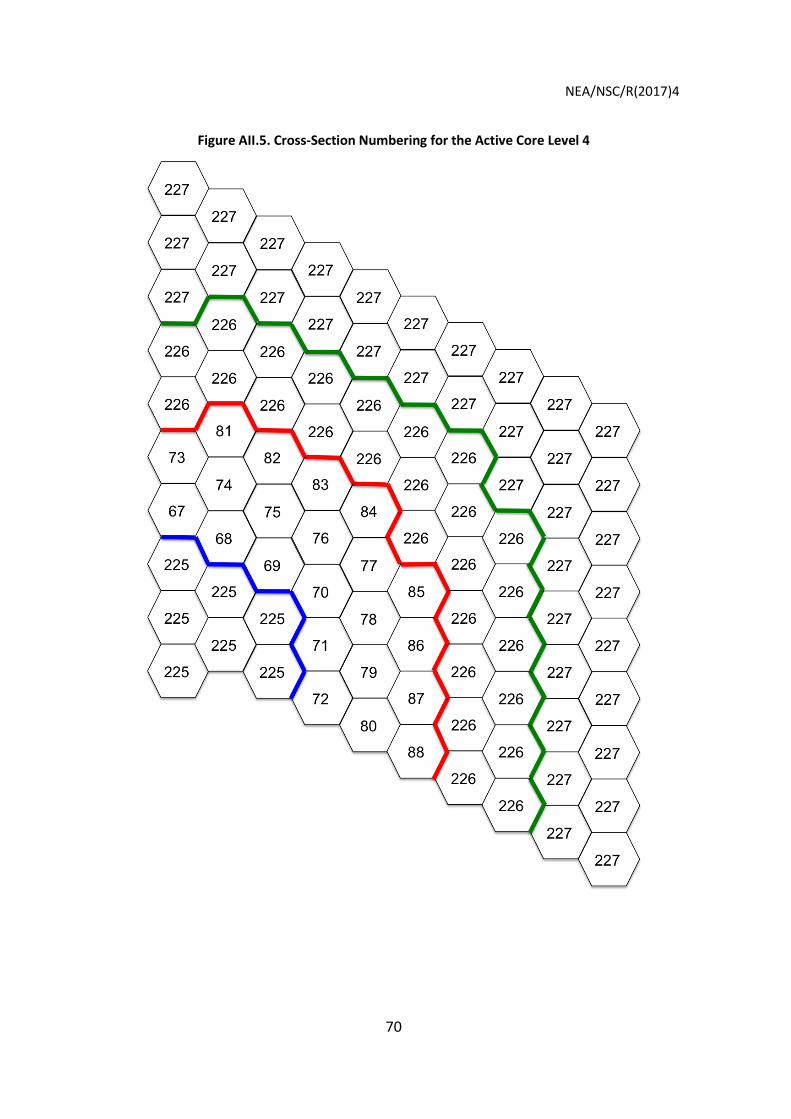
NEA/NSC/R(2017)4

70


NEA/NSC/R(2017)4

71


NEA/NSC/R(2017)4

72


NEA/NSC/R(2017)4

73


NEA/NSC/R(2017)4

74


NEA/NSC/R(2017)4

75


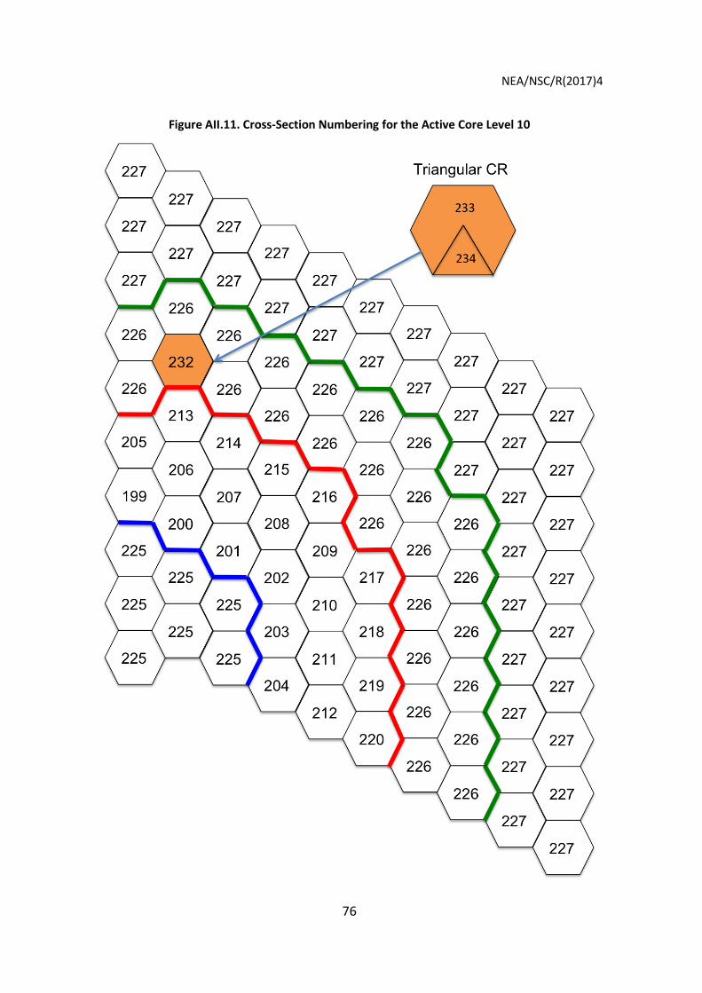
NEA/NSC/R(2017)4

76


NEA/NSC/R(2017)4

77

Figure AII.12. Cross-Section Numbering for the Top Reflector

NEA/NSC/R(2017)4

78

Appendix III. Four-parameter cross-section specifications

AIII-1. General tabulation information

• title;

• decay constant for the kth delayed precursor group;

• inverse neutron speed;

• core state point parameters;

• reflector state point parameters.

AIII-2. Material specific tabulation

For each fuel block in the core the following dataset is specified:

= normalised group flux used in homogenisation

ΣTg = total macro x-sec

ΣTrg

= transport x-sec

νΣ fg = nu fission macro x-sec

Σ fg = fission macro x-sec

χg = steady-state fission spectrum [both prompt and delayed]

χkD,g

= delayed fission spectrum for the kth delayed group

Σs0g'→ g

= P0 scattering matrix

Σs1g'→ g

= P1 scattering matrix

βk = delayed neutron fraction for the kth delayed group

κ = energy produced per fission

σag,Xe135

= microscopic absorption x-sec for 135Xe

γg,I135 = 135I fission yield

γg,Xe135= 135Xe fission yield

NEA/NSC/R(2017)4

79

Appendix IV. Thermo-physical properties

All temperatures in this section are in Kelvin, unless specified otherwise.

AIV-1. Fixed thermo-physical properties for steady-state Exercise 2a

The thermo-physical properties that should be used in the steady-state Exercise 2a are shown in Table AIV-1. If the steady-state solution of the thermal fluid equations is obtained via a null transient participants should use the heat capacities of the various materials at a temperature of 1,000 K. No porosity correction should be performed.

Table AIV.1. Fixed Thermo-Physical Properties

Material Conductivity Emissivities Fuel compact 20.0 0.85

Fuel block 37.0 0.85

Grade H-451 graphite 66.0 0.85

Grade 2020 graphite 35.0 0.85

Core Barrel

Core Restraint Element

MCSS Upper plenum thermal protection

17.8 0.85

Ceramic tile 0.91 0.85

Thermal insulation 0.175 0.85

RPV 40.0 0.85

Coolant 0.41 N/A

Air 0.068 N/A

AIV-2. Effective properties for TRISO particles

The effective thermal conductivity of the TRISO particles is computed with:

𝑘𝑒𝑓𝑓,𝑇𝑅𝐼𝑆𝑂 = 𝑘𝑚 �1 − 2𝐵(𝑁𝑐𝑜𝑎𝑡+2)

1 + 𝐵(𝑁𝑐𝑜𝑎𝑡+2)�

Where 𝑘𝑚 is the conductivity of the graphite matrix and 𝐵(𝑁𝑐𝑜𝑎𝑡+2) is the coefficient obtained from inverting the matrix system that represents the various TRISO coatings as developed by AMEC/NSS [6]. The actual matrix shown in the reference is in error. The correct matrix of the four coatings (Ncoat = 4) is given in Figure AIV.1.

NEA/NSC/R(2017)4

80

Figure AIV.1. Corrected Matrix for the AMEC Compact Model

⎣⎢⎢⎢⎢⎢⎢⎢⎢⎢⎢⎢⎢⎢⎢⎢⎢⎢⎢⎢⎢⎢⎢⎢⎡ 1 −1

1 −1

1 −1

1 −1

1 −1

1

𝑎53

𝑎13 − 𝑎5

3

𝑎13

𝑎(𝑁𝑐𝑜𝑎𝑡+1)3

𝑎23 − 𝑎5

3

𝑎23

𝑎53

𝑎33 − 𝑎5

3

𝑎33

𝑎53

𝑎43 − 𝑎5

3

𝑎43

1 −1

0

0

𝑘1 −𝑘2

𝑘2 −𝑘3

𝑘3 −𝑘4

𝑘4 −𝑘5

𝑘5 −𝑘6

1

−2 𝑎53

𝑎13 𝑘1 2 𝑎5

3

𝑎13 𝑘2

−2 𝑎53

𝑎23 𝑘2 2 𝑎5

3

𝑎23 𝑘3

−2 𝑎53

𝑎33 𝑘3 2 𝑎5

3

𝑎33 𝑘4

−2 𝑎53

𝑎43 𝑘4 2 𝑎5

3

𝑎43 𝑘5

−2𝑘5 2𝑘6⎦⎥⎥⎥⎥⎥⎥⎥⎥⎥⎥⎥⎥⎥⎥⎥⎥⎥⎥⎥⎥⎥⎥⎥⎤

The effective specific heat capacity is computed with a scheme based on balance of energy and the effective density with a scheme based on balance of mass:

𝐶𝑝𝑒𝑓𝑓 =∫𝜌𝐶𝑝𝑑𝑉∫𝜌𝑑𝑉

𝜌𝑒𝑓𝑓 =∫𝜌𝑑𝑉∫𝑑𝑉

AIV-3. Effective properties for fuel compacts

The thermal conductivity of fuel compacts is computed with:

𝑘𝑒𝑓𝑓, 𝑐𝑜𝑚𝑝𝑎𝑐𝑡 = 𝑘𝑚 �1 − 2𝛼𝐵(𝑁𝑐𝑜𝑎𝑡+2)

1 + 𝛼𝐵(𝑁𝑐𝑜𝑎𝑡+2)�

Where 𝑘𝑚 is the conductivity of the graphite matrix, 𝛼 is the volume fraction occupied by the TRISO particles and 𝐵(𝑁𝑐𝑜𝑎𝑡+2) is the coefficient obtained from inverting the matrix system that represents the various TRISO coatings [6].

The effective specific heat capacity is computed with a scheme based on balance of energy and the effective density with a scheme based on balance of mass, as shown above.

NEA/NSC/R(2017)4

81

AIV-4. Effective properties for thermal unit cells

The thermal conductivity model of the thermal unit cell is based on Maxwell’s theory of the conductivity of composite materials. The original theory is derived for two materials, but it is extended to three materials for the HTR applications by AMEC/NSS [5].

Figure AIV.2. Unit cell of MHGTR Fuel Block

The effective radial conductivity of the thermal unit cell shown in Figure AIV.2 is given with

the following expression:

𝑘𝑒𝑓𝑓

= 𝑘𝑠 �1

−2�𝛼1�𝑘𝑠 − 𝑘𝑝𝑜𝑟�(𝑘𝑠 + 𝑘𝐹𝐶) + 𝛼2(𝑘𝑠 − 𝑘𝐹𝐶)�𝑘𝑠 + 𝑘𝑝𝑜𝑟��

��𝑘𝑠 + 𝑘𝑝𝑜𝑟�(𝑘𝑠 + 𝑘𝐹𝐶) + 𝛼1�𝑘𝑠 − 𝑘𝑝𝑜𝑟�(𝑘𝑠 + 𝑘𝐹𝐶) + 𝛼2(𝑘𝑠 − 𝑘𝐹𝐶)�𝑘𝑠 + 𝑘𝑝𝑜𝑟��

where:

keff = effective radial thermal conductivity of the cell

ks = thermal conductivity of the graphite

kpor = thermal conductivity of the pore material

kFC = thermal conductivity of the fuel compact

α1 = volume fraction of gap material

α2 = volume fraction of fuel compacts

The effective axial conductivity of the thermal unit cell shown in Figure AIV.2 is given with the following expression:

𝑘𝑒𝑓𝑓,𝑎𝑥𝑖𝑎𝑙 = 𝑘𝑠𝛼3 + 𝑘𝐹𝐶𝛼2 + 𝑘𝑝𝑜𝑟𝛼1

where α3 =volume fraction of graphite

NEA/NSC/R(2017)4

82

The effective specific heat capacity is computed with a scheme based on balance of energy and the effective density with a scheme based on balance of mass:

𝐶𝑝𝑒𝑓𝑓 =∫𝜌𝐶𝑝𝑑𝑉∫𝜌𝑑𝑉

𝜌𝑒𝑓𝑓 =∫𝜌𝑑𝑉∫𝑑𝑉

AIV-5. Grade H-451 graphite

The original MHTGR-350 graphite material H-451 was replaced by PCEA AG from another vendor, according to information verified with GA. The density of PCEA AG (1 850 kg/m3) has therefore been used for both the neutronic and thermal fluid specification, but since no information are available on the behaviour of PCEA AG under exposure to fluence, the thermal conductivity and specific heat capacity of H-451 graphite (sourced from the Graphite Handbook [12]) were assumed to apply to PCEA AG for the purposes of this benchmark.

Grade H-451 graphite is a near-isotopic, petroleum-coke-based, artificial graphite developed specifically for HTGR fuel element and reflector application [12]. Grade H-451 graphite is used in standard fuel, RSC fuel, and replaceable reflector blocks. The geometric descriptions of the fuel block are given in Volume I, Figures I-4, I-5, and I-6.

Temperature and fluence dependent conductivities are included in Table AIV-2. These polynomials fits have been developed from GA empirical correlations [12] based on an irradiation temperature of 1 200K. Conductivities for fluence levels that lie between the points provided can be linearly interpolated. Any value outside the temperature range of 300 K to 1 900 K and above a fluence of 8×1025 n/m2 will retain a constant value based on the closest value in the range of validity. For this benchmark the material thermodynamic properties are assumed isotropic.

Table AIV.2. Thermal Conductivity of Grade H-451 Graphite

Fluence [x1025 n/m2] Value* [W/m/K] Un-irradiated

k = 3.28248x10−5T 2 −1.24890x10−1T +1.692145x102

0.2

0.5 1 3 8 * Empirical data range [500K – 1800K], T in K

Other H-451 graphite thermal properties are shown in Table AIV-3. Graphical representations

of both the thermal conductivity and the specific heat capacity are included as reference material to the participant in Figures AIV.3 and AIV.4, respectively.

NEA/NSC/R(2017)4

83

Figure AIV.3. Thermal Conductivity of Grade H-451 Graphite

Table AIV.3. Grade H-451 Graphite Thermo-Physical Properties

Property Value* Density (kg/m3) 1 850

Specific Heat (J/kg/K)

Cp =0.54212 − 2.42667x10−6T − 90.2725T −1 − 43449.3T −2

+1.59309x107T −3 −1.43688x109T −4

⋅ 4184

Emissivity 0.85 * T in K

NEA/NSC/R(2017)4

84

Figure AIV.4. Specific Heat Capacity of Grade H-451 Graphite

AIV-6. Grade 2020 graphite

The large rectangular grade 2020 graphite is fine-grained, molded artificial graphite produced in large rectangular blocks [12]. It is the reference material for permanent side reflectors and central reflector column support blocks.

Temperature and fluence dependent conductivities are included in Table AIV-4. Conductivities for fluence levels that lie between the points provided can be linearly interpolated. These polynomials fits have been developed from GA empirical correlations [12] in the range of the empirical data. An exponential tail has been added for conservatism to temperatures beyond 1 000 K in order to extend the domain up to 2 000 K. This assumption should reduce the effective heat transfer from the reflector during heat up accidents. Note that the magnitude of the fluence is different than that provided for the H-451 graphite, 1022 versus 1025 n/m2. Any value outside the temperature domain [300 K – 2 000 K] and above the fluence range of 2 × 1023 n/m2 will retain a constant value based on the closest value. A graphical representation of the thermal conductivity of grade 2020 graphite is shown in Figure AIV-5. The plot displays the domain of experimental data for both un-irradiated and irradiated graphite. Other grade 2020 graphite thermal properties are shown in Table AIV-5. The specific heat capacity of grade 2020 graphite is the same as grade H-451 and all other graphites. For this benchmark the material thermodynamic properties are assumed isotropic.

NEA/NSC/R(2017)4

85

Table AIV.4. Thermal Conductivity of Grade 2020 Graphite

Fluence (1022 n/m2)

Thermal Conductivity Value (W/m/K)

Un-irradiated k*= 1.71039E-7T3-3.73458E-4T2+2.18725E-1T+2.65411E+1 [300 K -1000 K] k= 58.800*EXP(-3.365E-4*T) [1000 K – 2000 K]

0.4 k=-0.0263158T+69.71052632 [300 K -673 K] k**= 5.89227E-5T2-1.28522E-1T+1.11808E+2 [673 K -1000 K] k= 70.560*EXP(-5.188E-4*T) [1000 K – 2000 K]

1 k**= 7.53255E-6T2-3.46161E-2T+6.98153E+1 [300 K -1000 K] k= 73.087*EXP(-5.781E-4*T) [1000 K – 2000 K]

4 k**= -1.26995E-05T2+1.08450E-02T+4.32150E+01 [300 K -1000 K] k= 74.219*EXP(-6.057E-04*T) [1000 K – 2000 K]

10 k**= 39.55224 [300 K -650 K] k**= -2.87164E-05T2+4.83551E-02T+2.02541E+01 [650 K -1000 K] k= 72.429*EXP(-6.190E-04*T) [1000 K – 2000 K]

20 k**= 34.34069 [300 K -650 K] k**= -4.29785E-05T2+8.18658E-02T-7.13659E-01 [650 K -1000 K] k= 69.758*EXP(-6.075E-4*T) [1000 K – 2000 K]

*Empirical data - range of validity [295K – 1073K]

**Empirical data - range of validity [673K – 1073K]

Table AIV.5. Grade 2020 Graphite Thermo-Physical Properties

Property Value Density (kg/m3) 1 780

Specific Heat (J/kg/K) same as H-451

Emissivity 0.85

NEA/NSC/R(2017)4

86

Figure AIV.5. Thermal Conductivity of Grade 2020 Graphite

AIV-7. Pyrolitic carbon layer

The TRISO particles include an outer and IPyC layer that surrounds the SiC layer, which provide structural support. A porous carbon layer is positioned between the kernel and the IPyC to retain fission gases. The thermo-physical properties of the PyC and porous carbon layers are included in Table AIV-6. The thermal conductivity measurements of isotropic pyrolitic carbon performed by Bokros et al. [14] were fitted into a power law equation. The sample parameters were: a Bacon Anisotropy Factor of 1.00, a density of 1 930 kg/m3, and a layer spacing of 3.410 Å. The porosity correction factor is determined with the simplified Maxwell-Eucken model [16]. The irradiation correction factor was derived from matrix materials in the Jülich programme [13] and it is assumed to be applicable to the PyC. The porous carbon conductivity uses the same correlation as the PyC, but it is further divided by a factor of two to yield values in the range specified in the Jülich programme.

Graphical representations of the thermal conductivity in the pyrolitic and porous carbon layers are included as reference material to the participant in Figures AIV.6 and AIV.7, respectively.

NEA/NSC/R(2017)4

87

Table AIV.6. Pyrolitic and Porous Carbon Thermo-Physical Properties

Property Value*

Thermal Conductivity(W/m/K)

=neutron fluence in 1025 n/m2 DNE

Density PyC (kg/m3) 1 900

Density Porous C (kg/m3) 970

Specific Heat (J/kg/K) same as H-451 *T in K

Figure AIV.6. Thermal Conductivity of Pyrolitic Carbon

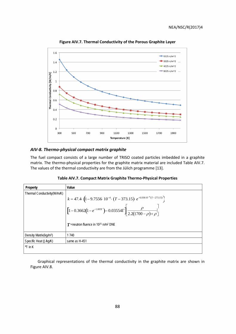
NEA/NSC/R(2017)4

88

Figure AIV.7. Thermal Conductivity of the Porous Graphite Layer

AIV-8. Thermo-physical compact matrix graphite

The fuel compact consists of a large number of TRISO coated particles imbedded in a graphite matrix. The thermo-physical properties for the graphite matrix material are included Table AIV.7. The values of the thermal conductivity are from the Jülich programme [13].

Table AIV.7. Compact Matrix Graphite Thermo-Physical Properties

Property Value Thermal Conductivity(W/m/K)

k = 47.4⋅ 1− 9.7556⋅ 10−4 ⋅ T − 373.15( )⋅ e−6.036⋅10−4 T −273.15( )( )1− 0.3662 1− e−1.005Γ( )− 0.03554Γ[ ] ρ

2.2 1700 − ρ( )+ ρ

=neutron fluence in 1025 n/m2 DNE

Density Matrix(kg/m3) 1 740 Specific Heat (J/kg/K) same as H-451

*T in K

Graphical representations of the thermal conductivity in the graphite matrix are shown in

Figure AIV.8.

NEA/NSC/R(2017)4

89

Figure AIV.8. Thermal Conductivity of the Carbon Matrix

AIV-9. SiC layer

The SiC layer is an essential constituent of the TRISO particle. It provides the fission product barrier against release. The thermo-physical properties are shown in Table AIV-8. The temperature dependent thermal conductivity is obtained from the Jülich programme [13,15]. Irradiation effects on the thermal conductivity of SiC are quite dramatic. A reduction of 50-70% was documented at an irradiation temperature of 1 100oC and a fluence of 4×1025 n/m2 DNE (Dido Nickel Equivalent) [18]. Since no clear fluence and temperature dependent correlation exists to date, an exponential correlation is suggested by Ho for the irradiation dependent conductivity. The specific heat correlation was derived by Snead et al. [17].

Table AIV.8. SiC Thermo-Physical Properties

Property Value

Thermal Conductivity(W/m/K) 𝑘 = �

17885𝑇 + 2� 𝑒−0.1277𝛤 .

Density (kg/m3) 4 210

Specific Heat (J/kg/K)

Cp = 925.65 + 0.3772T − 7.9259x10−5T 2 −3.1946x107

T 2

= neutron fluence in 1025 n/m2 DNE units, T is in Kelvin.

Graphical representations of both the thermal conductivity and the specific heat capacity are included as reference material to the participant as in Figures AIV.9 and AIV.10, respectively.

Γ

NEA/NSC/R(2017)4

90

Figure AIV.9. Thermal Conductivity of the SiC Layer

Figure AIV.10. Specific Heat Capacity of the SiC Layer

AIV-10. UC0.5O1.5 kernel

Since no data is available for UC0.5O1.5., uranium dioxide properties will be used instead.

AIV-11. Thermal conductivity of UO2

The Lucuta model [19] for irradiated UO2 is:

[W/m/K]

NEA/NSC/R(2017)4

91

where:

T = temperature [K]

B = burn-up [at. %]

P = porosity of UO2 [unit less]

ρ = density of UO2 [kg/m3]

ρTD = theoretical density of UO2 [kg/m3]

ko = conductivity of 100% dense UO2 [W/m/K]

FD = dissolved solid fission product factor [unit less]

FP = precipitated solid fission product factor [unit less]

FR = radiation damage factor [unit less]

t =T(K)1000

k0(T) =115.8

7.5408 +17.692t + 3.6142t 2 + 7410.5t −5 2e−16.35

t

FD =1.09B3.265 + 0.0643

TB

arctan

1.09B3.265 + 0.0643

TB

−1

FP =1+0.019B

3 − 0.019B1+ e

−(T −1200)100

−1

FR =1−0.2

1+ e(T −900)

80

AIV-12. Heat capacity of UO2

The specific heat capacity model covers the temperature range 298.15 K≤T<3120 K and it is functionalised as:

where:

Cp(T)=[J/kg/K]

NEA/NSC/R(2017)4

92

T = Temperature in K

C2(B) = 8.463x10−03(1+ 0.011* B)

B= burn-up in atom percent

AIV-13. Density of UO2

Participants should use the fixed value ρ(273)= 10970 kg/m3, if their model does not contain dimensionality changes for the kernel. For models that compute kernel expansion, the density as a function of temperature is calculated with:

3

)()273()273()(

=

TLLT ρρ [Kg/m3]

where:

ρ(273)= 10970 kg/m3, is the density of UO2 at 273 K. L(273) and L(T) are the lengths at 273 K and at temperature T(K), respectively.

For the temperature Range 273 K ≤ T <923 K,

L(T) = L(273)[ 9.9734x10-1 +(9.802x10-6)T - (2.705x10-10)T2 +(4.391x10-13)T3]

In the temperature Range 923 K ≤ T <3120 K,

L(T) = L(273)[ 9.9672x10-1 +(1.179x10-5)T - (2.429x10-9)T2 +(1.219x10-12)T3]

AIV-14. Core barrel/core restraint element/metallic core support structure/upper plenum thermal protection structure

The core barrel, CRE, MCSS, and UPTPS are made from Alloy 800 H. The thermo-physical properties for the core barrel are shown in Table AIV.9.

Table AIV.9. Core Barrel/CRE/MCSS/UPTPS Thermo-Physical Properties

MCSS / UPTPS Thermo-physical Properties Property Value Thermal Conductivity (W/m/K) 17.8 Density (kg/m3) 7 800 Specific Heat (J/kg/K) 515 Emissivity 0.85

AIV-15. Ceramic tile

The thermo-physical properties for the ceramic tile are shown in Table AIV.10.

NEA/NSC/R(2017)4

93

Table AIV.10. Ceramic Tile Thermo-Physical Properties

Property Value Thermal Conductivity (W/m/K) Density (kg/m3) 1 310 Specific Heat (J/kg/K) 1 100 Emissivity 0.85

AIV-16. Thermal insulation

The thermo-physical properties for the thermal insulation used in the cross-duct and in the UPTPS are shown in Table AIV.11.

Table AIV.11. Thermal Insulation Thermo-Physical Properties

Property Value Thermal Conductivity (W/m/K) 0.0249 T101 + T101.0 427 −= −− xxk Density (kg/m3) 128 Specific Heat (J/kg/K) 1 130 Emissivity 0.85

AIV-17. Pressure vessel

The reactor vessel consists of plates made of SA-533B Class I steel, and forgings from SA-508 Class 3 steel, designed to Section III of the ASME Boiler and Pressure Vessel Code. The thermo-physical properties for the pressure vessel are shown Table AIV.12.

Table AIV.12. Pressure Vessel Thermo-Physical Properties

Property Value Thermal Conductivity (W/m/K) 40.0 Density (kg/m3) 7 500 Specific Heat (J/kg/K) 580 Emissivity 0.85 Effective emissivity 0.74* *Note that an effective emissivity can be used to model the RPV and the air gap in the reactor cavity, as an alternative to applying a RCCS emissivity of 0.80..

AIV-18. Coolant (helium)

The thermo-physical properties of the helium coolant are included in Table AIV.13.

NEA/NSC/R(2017)4

94

Table AIV.13. Helium Coolant Thermo-Physical Properties

Property Value Thermal Conductivity(W/m/K)

k = 2.682x10−3 × 1+1.123x10−8 × P( )× TC

where:

C = 0.71× 1− 2.0x10−9 × P( )

[P in Pa]

Density (kg/m3) ideal gas use R=8.314 m3Pa/K/mol M=4.002 g/mol

Specific Heat (J/kg/K) Cp=5195 Dynamic Viscosity (kg/m/s)

𝜇 = 3.674𝑥10−7𝑇0.7

Nusselt Number Correlation [20]

𝑁𝑢 = 0.021 ∗ 𝑅𝑒0.8𝑃𝑟0.4 �𝑇𝑤𝑇𝑏�−0.5

AIV-19. Air

The thermo-physical properties for air are included in Table AIV-14. The air pressure outside the core is assumed to be one atmosphere.

Table AIV.14. Air Thermo-Physical Properties

Property Value Thermal Conductivity(W/m/K) Density (kg/m3)

Specific heat (J/kg/K)

NEA/NSC/R(2017)4

95

Appendix V. Hexagonal to cylindrical conversion for the permanent reflector

The final results of the benchmark will be reported with a cylindrical permanent reflector region. A conversion method from hexagonal to cylindrical representation of the permanent reflector region is included in this section since the participants’ results can be reported with either representation. Figure V.1 shows an overlay of the hexagonal numbering on the cylindrical representation.

Figure V.1. Overlay of Hexagonal to Cylindrical Reporting Mesh

The values included in Table V.1 are used to convert the hexagonal representation to a

cylindrical representation of the permanent reflector regions.


Graphite)




Graphite)



Neutronic Boundary

Outside Air

120o Symmetry Line

1

2

4

8

3 7

13 21

57

5 6

12 20

30

56 72

9 10

11 19

29 41

55 71

14 15

16 17

18 28

40 54

22 23

24 25

26 27

39 53

32 33

34 35

36 37

38 52

44 45

46 47

48 49

50 51

58 59

60 61

62 63

64 65

74 75

76 77

78 79

80 81

90

89

88

87

86

85

84

83

70

69

68

67

66

82

73 91

2 4

8 14

32

3 5

9 15

23 33

45

7 6

10 16

24 34

46

13 12

11 17

25 35

47

21 20

19 18

26 36

48

31 30

29 28

27 37

49

43 42

41 40

39 38

50

57 56

55 54

53 52

3 5

9 15

23

45

7 6

10 16

24

46

13 12

11 17

25

47 35

21 20

19 18

26

48 36

31 30

29 28

27

49 37

43 42

41 40

39

50 38

57 56

55 54

53 52

2 4

8 14

22 32

44 58

74

4.72o 7.80o 8.53o

8.95o

8.95o

8.53o

7.80o

9.43o

7.80o

8.95o

8.95o

8.53o

8.53o

7.80o

4.72o

31 42

43 22

34

33

NEA/NSC/R(2017)4

96

Table V.1. Conversions from Hexagonal to Cylindrical Representation

The cross-sections for the RSC blocks already take into account the presence of the RSC hole at the block level. For triangular reporting of the flux, the six values for each block will be arithmetically averaged.

For the thermal fluids portion, the triangular reporting of values will assume that the regions with penetrations have reduced densities. Therefore, the thermal fluids solutions are volume weighted for blocks with penetrations. Participants are recommended to use reduced densities for RSC or controlled regions.

NEA/NSC/R(2017)4

97

Appendix VI. Fuel loading pattern

Reload segment A and B represent the locations with once-burned and twice-burned fuel at EOEC, respectively.

Figure VI.1. Fuel loading pattern

NEA/NSC/R(2017)4

98

Appendix VII. List of data files

Table VII.1 includes all of the data files that are provided to benchmark participants.

Table VII.1. Input Data Files

Filename Description Exercises OECD-MHTGR350_Simplified.xs Simplified cross-sections Steady-state Ex. 1 OECD-MHGTR350-power.inp Power density distribution Steady-state Ex. 2 OECD-MHGTR350-fluence.inp Fluence distribution Steady-state Ex. 2 & 3

Transient Ex. all OECD-MHGTR350-burnup.inp Burn-up distribution Steady-state Ex. 2 & 3

Transient Ex. all OECD-MHGTR350-decayheat.inp Decay heat distribution Transient Ex. 1, 2, & 3 Xsmap.pdf Sample core cross-section material map Steady-state Ex. 1 & 3

Transient Ex. All OECD-MHTGR350.xs 4th dimensional cross-section tables Steady-state Ex. 3

Transient Ex. all GA_Number_Densities.csv Number densities provided by GA for

each block N/A

NEA/NSC/R(2017)4

99

Appendix VIII. Auxilliary computer programs

All of the subroutines described in this section are available for benchmark participants. They are provided in the FORTRAN 90 language.

AVIII-1. Loaddist module

The loaddist module is included in loaddist.f90. It contains four subroutines: loadFBmaps, loadpower, loadDHmap, loadnSourcemap and DHinterpol. The first four routines load the various distributions provided for the benchmark exercises. DHinterpol linearly interpolates the decay heat data.

AVIII-1.1. Loadfbmaps

The subroutine loadFBmaps provided in file loaddist.f90 reads the fluence and burn-up maps for the active core region and translates them to a full core array.

The subroutine requires two temporary units (fluence_file,burn-up_file) for the two input text files that are read. It returns two full core arrays: fluence (12,91) and burn-up (12,91). The subroutine call specification for loadFBmaps is:

loadFBmaps(fluence_file,burn-up_file,fluence,burn-up)

AVIII-1.2. Loadpower

The subroutine loadpower provided in file loaddist.f90 reads the power density map for the active core region and translates it to a full core array. One power density value is provided for each fuel block.

The subroutine requires one temporary units (power_file) and returns one full core array power (12,91). The subroutine call specification for loadpower is:

loadpower(power_file,power)

AVIII-1.3. LoadDHmap

The subroutine loadDHmap provided in file loaddist.f90 reads the decay heat map for the active core region and translates it to a full core array.

The subroutine requires one temporary unit (dh_file) for the input text file that is read. It loads the decay heat data into the derived type decay heat (137), which is later used by the linear interpolator in subroutine DHintepol. The derived type includes:

decay heat(i)%time time

decay heat(i)%DH(12,91) decay heat power density

The subroutine call specification for loadDHmap is:

loadDHmaps(dh_file)

AVIII-1.4. LoadDCCsourcemap

The subroutine loadDCCSourcemap provided in file loaddist.f90 reads the neutron source map for the active core region and translates it to a full core array. One source value is provided for each fuel block.

NEA/NSC/R(2017)4

100

The subroutine requires one temporary units (DCCsource_file) and returns one full core array DCCsource(12,91). The subroutine call specification for loadDCCSource is:

loadDCCSource(DCCSource_file,DCCsource)

AVIII-1.5. DHinterpol

The subroutine DHinterpol provided in file loaddist.f90 linearly interpolates the decay heat data.

The subroutine requires the time at which the interpolation is to be performed (mtime) and returns a full core distribution with the decay heat density DHdist(12,91). The subroutine call specification for DHinterpol is: DHinterpol(mtime,DHdist)

AVIII-2. MTPlook module

The mtplook module, which is included in file mtplook.f90, contains a series of subroutines to compute the various thermo-physical properties for material regions used in the benchmark. There are two subroutines used to compute basic properties, tplook and HeCool. In addition, various calculators are included to determine effective properties for the TRISO particles, fuel compacts, and thermal unit cells (CompactTP and CellTP).

AVIII-2.1. TPlook subroutine

The subroutine tplook calculates the solid material thermo-physical properties of the core constituents listed in Table AVIII.1.

Table VIII.1. Solid Material

Tplook Material Number Description

1 H-451 Graphite Block 2 2020 Graphite Block 3 Core Barrel 4 Pressure Vessel 5 Core Restraint Element / Metallic Core Support Structure/Upper Plenum Thermal Protection

Structure 6 UO2\UC[0.5]O[1.5] Kernel 7 Porous Carbon layer 8 PyC 9 SiC 10 Compact Matrix 11 Air 12 Ceramic tile 13 Thermal insulation

The input required for tplook is a “material number” from Table VIII.1 along with its average

temperature in [K], burn-up [at. %], and fluence values [n/m2 Equivalent DIDO Nickel Dose (EDND)]. The burn-up and fluence values should be based on the the burn-up and fluence distributions provided. The subroutine returns the material’s density [kg/m3], conductivity [W/m/K], specific heat capacity [J/kg/K], and emissivity [unitless], if applicable.

The subroutine call specification for tplook is:

tplook(mat,tav,bnp,flu,rho,k,cp,emis)

NEA/NSC/R(2017)4

101

AVIII-2.2. HeCool subroutine

The subroutine HeCool is also included in file tplook.f90 and it calculates the thermo-physical properties for the helium coolant. The input parameters are helium temperature [K] and pressure [Pa]. The subroutine returns the helium conductivity [W/m/K], specific heat capacity [J/kg/K], density [kg/m3], and dynamic viscosity [kg/m/s].

The subroutine call specification for HeCool is:

HeCool(T,P,k,cp,rho,vis)

AVIII-2.3. CompactTP subroutine

This subroutine uses the derived type compactdat for input and output. In addition, the compactdat derived type includes a trisodat derived type named “triso” that is used to characterise the average TRISO properties in the compact. The subroutine computes both TRISO and compact effective thermo-physical properties. The effective densities and specific heat capacities are volume weighted. The effective conductivities are computed using the AMEC method delineated in Appendix IV.

compactdat%triso%Tlay(nlay) 5 layer temperatures

compactdat%triso%rvol(nlay) 5 layer relative volumes

compactdat%triso%burn-up UCO burn-up

compactdat%triso%fluence graphite fluence

compactdat%triso%rho TRISO effective density

compactdat%triso%k TRISO effective conductivity

compactdat%triso%cp TRISO effective specific heat capacity

compactdat%rvol triso | matrix relative volume

compactdat%Tmatrix Compact matrix temperature

compactdat%rho Compact effective density

compactdat%k Compact effective conductivity

compactdat%cp Compact effective specific heat capacity

The subroutine call specification for CompactTP is:

CompactTP(compactdat)

AVIII-2.4. CellTP subroutine

This subroutine uses the derived type celldat for input and output. The celldat derived type includes a compactdat derived typed named “compact”. The subroutine will compute all effective thermo-physical properties for the TRISO, compact, and thermal cell. The effective cell density and specific heat capacity are computed with a volume-weighting scheme. The effective radial cell conductivity is obtained via Maxwell’s law. The thermal cell and Maxwell’s law are discussed in Appendix IV.

celldat%compact compactdat derived type

NEA/NSC/R(2017)4

102

celldat%rvol fuel|coolant|cell graphite relative volumes

celldat%TH451 H-451 graphite temperature

celldat%Tcool Coolant temperature

celldat%Pav Coolant pressure

celldat%rho Cell effective density

celldat%kradial Cell effective radial conductivity

celldat%kaxial Cell effective axial conductivity

celldat%cp Cell effective specific heat capacity

The subroutine call specification for CellTP is:

CellTP(celldat)

AVIII-3. XSlook module

The subroutine xslook included in file xslook.f90 is provided to load the simplified cross-section set included in OECD-MHTGR350_Simplified.xs. The user will need to interface with this program to transfer the data to their respective code structures. Xslook requires the specification of a temporary unit number and it returns a derived type xsdata array that contains the necessary data for the neutronics solver. On exit the array xstab includes the data below for all 234 core material regions, where i is the index for the core material and n is the index for the energy group.

xstab(i)%flux(n) normalised neutron flux

xstab(i)%sigt(n) total macroscopic cross-section

xstab(i)%diffco(n) isotropic diffusion coefficient

xstab(i)%nusigf(n) nubar * fission macroscopic cross-section

xstab(i)%sigf(n) fission macroscopic cross-section

xstab(i)%scat0(n,n) isotropic scattering macroscopic cross-section

xstab(i)%scat1(n,n) linear anisotropic macroscopic cross-section

xstab(i)%chi(n) neutron spectrum

The subroutine call specification for XSlook is:

XSlook(xs_file,xstab)

AVIII-4. XSlookTR module

The module xslookTR.f90 is provided to load and interpolate the cross-sections from the four parameter cross-section tables OECD-MHTGR350.xs. The following calls are needed for benchmark participants to interpolate the cross-sections:

• tabload(iunit), where iunit is a temporary unit to read the ASCII tabulation.

Note that the precursor decay constants and inverse velocities are loaded at this point into real arrays lambda() and invvel(), respectively.

NEA/NSC/R(2017)4

103

• corexsinterpol(mat,STpoint,tabcore), where the integer mat is the active core material id (1-220), STpoint is a real array with the four state point entries: fuel temperature, moderator temperature, Xe concentration, and H1 concentration, respectively. Tabcore is a fuelregionXS derived type that contains the data below, where n is the index for the neutron energy groups and np is the index for the neutron precursor groups.

abcore%flux(n) normalised neutron flux tabcore%SIGT(n) total macroscopic cross-section tabcore%SIGTR(n) isotropic transport cross-section tabcore%nuSIGF(n) nubar * fission macroscopic cross-section tabcore%SIGF(n) fission macroscopic cross-section tabcore%CHI(n) steady-state fission neutron spectrum (prompt+delayed) tabcore%CHID(n,np)=0 delayed fission neutron spectrum tabcore%SCAT0(n,n)=0 P0 scattering matrix tabcore%SCAT1(n,n)=0 P1 scattering matrix tabcore%Beta(np)=0 delayed neutron fraction tabcore%kappa=0 Energy produced per fission tabcore%sigaXe(n)=0 microscopic absorption Xe-135 tabcore%Xyield(n)=0 135Xe yield tabcore%Iyield(n)=0 135I yield

• refxsinterpol(mat,Tm,tabref), where the integer mat is the reflector or control rod material

id (221-234), Tm is a real variable with the material temperature. Tabref is a nonfuelregionXS derived type that contains the data below, where n is the index for the neutron energy groups and np is the index for the neutron precursor groups.

tabref%flux(n) normalised neutron flux tabref%SIGT(n) total macroscopic cross-section tabref%SIGTR(n) isotropic transport cross-section tabcore%SCAT0(n,n)=0 P0 scattering matrix tabcore%SCAT1(n,n)=0 P1 scattering matrix

In addition, the xslookTR module includes several auxiliary subroutines using by the main

subroutines to successfully load and interpolate the data and are described in Table VIII.2.

Table VIII.2. List of Subroutines in XslookTR

Procedure Name Procedure Description Tabload Loads the full tabulation into memory Indexing Reads the order of the state points from the ASCII file OECD-MHTGR350.xs and creates the

indexing that will be used for the interpolation Orgdat Sorts the data points used in the tabulation Loadfuel Loads the fuel region data Loadref Loads the reflector and control rod data Checkdat Verifies the tabulation order Corexsinterpol Interpolates the core region data Refxsinterpol Interpolates the reflector and control region data Findbound Find the bounding values for an interpolation point Polvol Calculated the polotype volume used for interpolating a data set Int4d Calculates the interpolation value

NEA/NSC/R(2017)4

104

Appendix IX. Brief XML tutorial

XML is a mark-up language that is used to store data in a self-explanatory manner. Data are managed hierarchically with the nature of the XML tree structure. Making the data “self-explanatory” is achieved by labelling elements. A sample XML tree is shown below.

XML>

<Header>

<File-ID>

<Contact>Javier Ortensi </Contact>

<Institution> Idaho National Laboratory </Institution>

<Country>US</Country>

<Time-stamp Date=”2012-01-09” Time=”15:00:00”> </Time-stamp>

<Computer code>INSTANT</Computer code>

<Computer code-description > INSTANT is a neutron transport code …

</Computer code-description >

<Kconvg> 1E-6</Kconvg>

<Fconvg> 1E-4</Fconvg>

<Method>Finite Element</Method>

<Model>PN transport n=1</Model>

<Format-type> Triangle</Format-type>

<PR-type>Cyl</PR-type>

<Num-blocks>2</Num-blocks>

<Data-name> Neutron-flux </Data-name>

</File-ID>

</Header>

</XML>

A tag is just a generic name for a <element>. An opening tag looks like <element>, while a closing tag has a slash that is placed before the element’s name: </element>. All information that belongs to an element must be contained between the opening and closing tags of an element.

NEA/NSC/R(2017)4

105

<mydistribution>1.000 1.000 1.000 1.000 1.000 1.000 1.000 </mydistribution >

If a tag is nested, then indentation is often used for readability.

<Data-body>

<mydistribution>1.000 1.000 1.000 1.000 1.000 1.000 1.000 </mydistribution >

</Data-body>

Attributes are used to specify additional information about the element. An attribute for an element appears within the opening tag. If there are multiple values an attribute may have, then the value of the attribute must be specified.

<Data-block ID =” 1” time=”0.0”>

Comments can be inserted when demanded with the paired ’<!–’ and ’’–-- This is a comment-->

NEA/NSC/R(2017)4

106

Appendix X. Benchmark participants

Contact Name Organisation Country Javier Ortensi Gerhard Strydom Sonat Sen

Idaho National Laboratory (INL) United States

Volkan Seker University of Michigan United States Kostadin Ivanov Ivor Clifford Jason Hou

Pennsylvania State University United States

Hyun Chul Lee Nam-il Tak Tae Young Han

Korea Atomic Energy Research Institute (KAERI) Korea

Hyung Jin Shim Seoul National University Korea Ulrich Rohde Emil Fridman Yurii Bilodid

Helmholtz-Zentrum Dresden-Rossendorf (HZDR) Germany

Armin Seubert Gesellschaft für Anlagen- und Reaktorsicherheit (GRS) Germany

NEA/NSC/R(2017)4

107

References

[1] NEA (2007), “PBMR Coupled Neutronic/Thermal Hydraulics Transient Benchmark: The PBMR-400 Core Design”, Draft 07 (2007), June 2007 (Vol.1: The Benchmark Definition has been published as NEA/NSC/DOC(2013)10 in July 2013), OECD, Paris.

[2] Neylan, A.J. et al. (1988), “The Modular High-Temperature Gas-Cooled Reactor (MHTGR) in the US”, Nuc. Eng. & Des. Vol. 109, pp. 99-105.

[3] General Atomics (2009), “Final Report – NGNP Core Performance Analysis, Phase 2”, Report 911184, Rev. 0.

[4] DOE-HTGR-90406 (1994), “MHTGR Nuclear Physics Benchmarks” Rev. 0, General Atomics.

[5] “Investigation of Local Heat Transfer Phenomena in a Prismatic Modular Reactor Core”, NR001/RP/001 R1, AMEC NSS Limited, March 2009.

[6] “Investigation of Local Heat Transfer Phenomena in a Pebble Bed HTGR Core” NR001/RP/002 R1, AMEC NSS Limited, March 2009.

[7] Bechtel GA Technologies et al. (1992), “Preliminary Safety Information Document for the Standard MHTGR”, MHTGR-86-024, Rev. 13.

[8] GA Technologies (1986), “Probabilistic Risk Assessment of the Modular HTGR Plant”, HTGR-86-011, Rev. 1 Draft.

[9] Lohnert, G. (1992), “The Consequences of Water Ingress into the Primary Circuit of an HTR-Module – From Design Basis Accident to Hypothetical Postulates”, Nuclear Engineering and Design, Vol. 134, pp. 159-176.

[10] DeHart, M.D. and A. P. Ulses (2009), “Benchmark Specification for HTGR Fuel Element Depletion,” NEA/NSC/DOC(2009)13, Paris, France.

[11] DIN 25485, “Decay heat power in nuclear fuels of high-temperature reactors with spherical fuel elements”, May 1990.

[12] General Atomics (1988), “Graphite Design Handbook”, DOE-HTGR-88111, Rev. 0.

[13] Gontard, R. and H. Nabielek (1990), “Performance Evaluation of Modern HTR TRISO Fuels”, HTA-IB-05/90, Jülich.

[14] Bokros, J.C. et al. (1968), Research on Graphite, GA-9099.

[15] Nabielek, H., K. Fukuda, K. Miato, T. Ogawa (1992), “Calculation of Particle Temperatures in NSRR Tests”, JAERI, unpublished draft.

[16] Biancheria, A. (1966), “The Effect of Porosity on Thermal Conductivity of Ceramic Bodies,” Transactions of the American Nuclear Society, 9, p. 15.

NEA/NSC/R(2017)4

108

[17] Snead, L.L. et al. (2007), “Handbook of SiC properties for fuel performance modeling”, J. Nucl. Sci. 371 (2007) 329-377.

[18] Ho, F.H. et al. (1993), “Material models of Pyrocarbon and Pyrolityc Silicon Carbide”, CEGA-002820, Rev. 1.

[19] Popov, S.G., J.J. Carbajo (2000), “Thermo physical Properties of MOX and UO2 Fuels Including the Effects of Irradiation”, ORNL/TM-2000/351.

[20] McEligot, D.M. et al. (2006), “Investigation of Fundamental Thermal-Hydraulic Phenomena in Advanced Gas-Cooled Reactors”, INL/EXT-06-11801.

Bibliography

[1] Massimo, L. (1976), “Physics of High-Temperature Reactors”, 1st ed., Pergamon Press Oxford.

[2] Duderstadt, J.J.,L.J. Hamilton (1976), “Nuclear Reactor Analysis”, 1st ed., John Wiley & Sons.

Documents

Benchmark of the Modular High-Temperature Gas-Cooled