EPA/100/R-12/001 June 2012

Benchmark Dose Technical Guidance

Risk Assessment Forum U.S. Environmental Protection Agency

Washington, DC 20460

ii

DISCLAIMER

This document has been reviewed in accordance with the U.S. Environmental Protection

Agency's peer and administrative review policies and approved for presentation and publication. Mention of trade names or commercial products does not constitute endorsement or recommendation for use.

iii

TABLE OF CONTENTS LIST OF FIGURES ........................................................................................................................ v LIST OF ABBREVIATIONS AND ACRONYMS ...................................................................... vi AUTHORS, TECHNICAL PANEL, AND STAFF ..................................................................... vii EXECUTIVE SUMMARY ......................................................................................................... viii 1. INTRODUCTION .............................................................................................................. 1

1.1. Purpose ................................................................................................................................ 1 1.2. Background ......................................................................................................................... 2 1.3. A Brief Review of Literature Relating to Benchmark Dose ............................................... 8

1.3.1. Earlier Uses of Benchmark Modeling in Dose-response Assessment .................. 8 1.3.2. Properties of the Benchmark Dose ........................................................................ 9 1.3.3. Approaches to BMD Computation ...................................................................... 10 1.3.4. Historical Development of this Benchmark Dose Technical Guidance .............. 11

2. BENCHMARK DOSE GUIDANCE ................................................................................ 12

2.1. Data Evaluation ................................................................................................................. 12 2.1.1. Study Design ....................................................................................................... 13 2.1.2. Aspects of Data Reporting .................................................................................. 13 2.1.3. Selection of Studies to be Modeled ..................................................................... 14 2.1.4. Selection of Endpoints to be Modeled ................................................................ 14 2.1.5. Minimum Dataset for Calculating a BMD .......................................................... 15 2.1.6. Combining Data for a BMD Calculation ............................................................ 18 2.1.7. Dosimetric Adjustments....................................................................................... 19

2.2. Selection of the Benchmark Response Level (BMR) ....................................................... 19 2.2.1. Quantal (Dichotomous) Data ............................................................................... 20 2.2.2. Continuous Data................................................................................................... 21

2.3. Modeling the Data............................................................................................................. 24 2.3.1. Introduction ......................................................................................................... 24 2.3.2. Background for Model Selection ........................................................................ 26 2.3.3. Selecting the Model ............................................................................................. 26 2.3.3.1. Type of endpoint ..................................................................................... 27 2.3.3.2. Experimental design................................................................................ 28 2.3.3.3. Constraints and covariates ...................................................................... 29 2.3.4. Model Fitting ....................................................................................................... 31 2.3.5. Assessing How Well the Model Describes the Data ........................................... 33 2.3.6. Improving Model Fit ............................................................................................ 34 2.3.7. Comparing Models .............................................................................................. 36 2.3.8. Calculating Confidence Limits to Get a BMDL ................................................. 37 2.3.9 Selecting the model to use for POD computation ............................................... 39

2.4. Reporting Recommendations ............................................................................................ 40 2.5. Decision Tree .................................................................................................................... 41

APPENDIX A. EXAMPLES ........................................................................................................ 43

A.1 Modeling Quantal Data ..................................................................................................... 43 A.1.1. Selecting models to fit (Section 2.3.3) .................................................................. 44

iv

TABLE OF CONTENTS (continued) A.1.2. Evaluating goodness-of-fit (Section 2.3.5) ........................................................... 44 A.1.3. Comparing Models (Section 2.3.7) ....................................................................... 45 A.1.4. Selecting a model to use as the basis for a POD (see Section 2.3.9) .................... 47

A.2. Quantal Data: Dropping Dose Groups (see Section 2.3.6) ............................................... 47 A.3. Continuous Data: Getting a Well-Fitting Model .............................................................. 51 A.4. Cancer Bioassay Data: Modeling to Obtain a POD for Linear Extrapolation .................. 57 A.5. Developmental Toxicity Data ........................................................................................... 62 A.6. Human Data ...................................................................................................................... 64

APPENDIX B. GLOSSARY ........................................................................................................ 66 APPENDIX C. SELECTED BENCHMARK DOSE MODELS .................................................. 76 APPENDIX D. BENCHMARK DOSE TECHNICAL GUIDANCE DOCUMENT CONTRIBUTORS AND REVIEWERS ...................................................................................... 79 REFERENCES ............................................................................................................................. 81

v

LIST OF FIGURES

1. Example of a model fit to dichotomous data, with BMD and BMDL indicated. ................... 7 2A. Flowchart of data evaluation steps for determining BMD modeling feasibility. ................... 16 2B. Illustrations of Datasets A, B, C corresponding to Figure 2A. .............................................. 17 3. Difference in population tail probabilities resulting from a one standard deviation shift

in the mean from a standard normal distribution, illustrating the theoretical basis for a baseline BMR of 1 SD. .......................................................................................................... 23

4. BMD decision tree. ................................................................................................................ 42

vi

LIST OF ABBREVIATIONS AND ACRONYMS AIC Akaike information criterion AUC area-under-the-curve BMC benchmark concentration BMCL benchmark concentration lower bound BMD benchmark dose BMDL benchmark dose lower bound BMDS BenchMark Dose Software BMDU benchmark dose upper bound BMR benchmark response CI confidence interval ED effective dose GEE generalized estimating equations HED human equivalent dose IRIS Integrated Risk Information System LED effective dose lower bound LOAEL lowest observed adverse effect level MLE maximum likelihood estimate NOAEL no observed adverse effect level PBPK physiologically based pharmacokinetic POD point of departure RfC reference concentration RfD reference dose SD standard deviation SE standard error UCL upper confidence limit UED effective dose upper bound UF uncertainty factor U.S. EPA United States Environmental Protection Agency

vii

AUTHORS, TECHNICAL PANEL, AND STAFF

AUTHORS This document was prepared by a technical panel under the auspices of U.S. EPA’s Risk Assessment Forum. The document reflects a consideration of comments received from an external peer review panel and members of the public, provided at a public peer review workshop meeting held on December 7–8, 2000, and of comments received and experiences gained in applying the methodology since that time. In addition, the document reflects consideration of additional comments received from intra-agency scientist review (2006−2008) and informal interagency review (2009−2011). TECHNICAL PANEL David Gaylor (Former Employee), U.S. Food and Drug Administration, Rockville, MD 20857 Jeff Gift, Office of Research and Development, U.S. EPA, Research Triangle Park, NC 27711 Karen Hogan (Lead), Office of Research and Development, U.S. EPA, Washington, DC 20460 Jennifer Jinot, Office of Research and Development, U.S. EPA, Washington, DC 20460 Carole Kimmel (Former Employee and Former Lead), Office of Research and Development, U.S. EPA, Washington, DC 20460 R. Woodrow Setzer (Former Lead), Office of Research and Development, U.S. EPA, Research Triangle Park, NC 27711 RISK ASSESSMENT FORUM STAFF Michael Broder, Office of the Science Advisor, U.S. EPA, Washington, DC 20460 Diane Henshel, Office of the Science Advisor, U.S. EPA, Washington, DC 20460

viii

EXECUTIVE SUMMARY The U.S. EPA conducts risk assessments for an array of health effects that may result from exposure to environmental agents. These assessments often include an analysis of the dose-response relationship between exposure and health-related outcomes. The dose-response assessment is essentially a two-step process: (1) defining a point of departure (POD) and (2) extrapolating from the POD for relevance to human exposure. The benchmark dose (BMD) approach, which involves dose-response modeling to obtain BMDs, i.e., dose levels corresponding to specific response levels near the low end of the observable range of the data, incorporates and conveys more information than the No Observed Adverse Effect Level (NOAEL) or Lowest Observed Adverse Effect Level (LOAEL) process traditionally used for noncancer health effects. The approach is similar to that for determining the POD for cancer endpoints (U.S. EPA 2005a). As the Agency moves toward harmonization of approaches for cancer and noncancer risk assessment, the dichotomy between cancer and noncancer health effects is being replaced by consideration of mode of action and whether the effects of concern are likely to be linear or nonlinear at low doses. Thus, the purpose of this document is to provide guidance for the Agency and the outside community on consistent application of the BMD approach for deriving BMDs for a variety of uses, including the determination of PODs for different types of health effects data, whether a linear or nonlinear low-dose extrapolation is used. Other uses of BMDs include comparing relative potencies (e.g., across chemicals) or relative sensitivities (e.g., across different subpopulations). Note that BMD modeling is also applicable to other fields, such as ecological risk assessment; however, this document focuses on the dose-response modeling of health effects. This guidance discusses the computation of: BMDs, benchmark concentrations (BMCs) and their confidence limits; data requirements; dose-response analysis; and reporting recommendations that are specific to the use of BMDs or BMCs. The following convention for terminology has been adopted in this document: BMD is used generically to refer to the benchmark dose approach; in the specific cases of characterizing model results, BMD and BMC refer to central estimates. BMDL or BMCL refers to the corresponding lower limit of a one-sided 95% confidence interval on the BMD or BMC, respectively. This is consistent with the terminology introduced by Crump (1995) and with that used in the U.S. EPA’s BMD software (BMDS), which is freely available at http://epa.gov/NCEA/bmds/. Despite the similarity in names, this document is not specific to EPA’s BMDS software; recommendations here can apply to other software packages and other dose-response models. As indicated above, the BMD approach was developed as an alternative to the NOAEL/LOAEL approach that has been used for many years in dose-response assessment but that has recognized limitations. Nonetheless, there will continue to be a need for the

ix

NOAEL/LOAEL approach because not all data sets are amenable to BMD modeling (e.g., those resulting from incomplete data availability or from a lack of models that can describe a data set adequately).

The preference in selecting suitable models for dose-response modeling is to use those that are consistent with the biological processes relevant in a particular case. Such models can include explicit expression of biological processes (e.g., cell growth dynamics, saturable enzyme processes) or covariates of the responses under consideration (e.g., time of response). In the absence of a biologically-based model, dose-response modeling is largely a curve-fitting exercise. This document concerns the simpler dose-response models. Because the application of the BMD approach and the interpretation of the results can be technically challenging, it is recommended that BMD modeling be performed by or in collaboration with personnel expert in the statistical procedures and potential pitfalls of this type of analysis. This document discusses a number of issues that support consistent application of the BMD approach:

1) Determination of studies and endpoints on which to base BMD calculations;

2) Selection of the benchmark response value; 3) Choice of the model(s) to use in computing the BMD; 4) Model fitting, assessment of model fit, and model comparison; 5) Computation of the confidence limit for the BMD (i.e., the BMDL); and 6) Reporting recommendations for the presentation of BMD and BMDL computations.

Determining studies and endpoints on which to base BMD calculations. Following the hazard characterization and selection of endpoints to use for the dose-response assessment, the relevant studies for modeling and BMD analysis can be evaluated. Most studies that show a graded monotonic response with dose are amenable to BMD analysis, and the minimum dataset for calculating a BMD should show a biologically or statistically significant dose-related trend in the selected endpoint(s). Having studies with one or more doses near the level of the BMR is desirable in order to give a better estimate of the BMD. Studies in which all the dose levels show changes compared with control values (i.e., there is no NOAEL) are generally readily useable in BMD analyses. This guidance provides definitions of commonly encountered types of data—most often, dichotomous (quantal) and continuous data—and discusses what information is needed in order to model the responses. For example, a dichotomous response may be reported as either the presence or absence of an effect, while a continuous response may be reported as an actual measurement or as a contrast (e.g., relative change from control). In the case of continuous data, when individual data are not available, the number of subjects, mean of the response variable, and a measure of response variability (e.g., standard deviation (SD), standard error (SE), or

x

variance) are needed for each group. Selected endpoints from different studies that are likely to be used in the dose-response assessment should all be modeled, especially if different uncertainty factors may be used for different studies and endpoints. The risk assessor evaluates the resulting BMDs and NOAELs/LOAELs (if some endpoints cannot be modeled) for use as PODs, using scientific judgment and principles of risk assessment as well as using the results of the modeling process. This guidance is limited to technical aspects of BMD modeling.

Selecting the benchmark response (BMR) value. The calculation of a BMD is directly determined by the selection of the BMR. Selecting BMRs involves making judgments about the statistical and biological characteristics of the dataset and about the applications for which the resulting BMDs/BMDLs will be used. Different uses may warrant different BMR values. The Agency does not currently have guidance to assist in making such judgments for the selection of the response levels, or BMRs, to use with BMD modeling for particular applications (e.g., for calculating reference doses or relative potency factors), and such guidance is beyond the scope of this document. Selections are made on a case-by-case basis, and for transparency a justification should be provided for each BMR selection. This guidance discusses general approaches for selecting the BMR(s) in the case of quantal data and continuous data.

For quantal data, an extra risk of 10% is the BMR for standard reporting (to serve as a basis for comparisons across chemicals and endpoints), and often for hazard ranking, since the 10% response is near the limit of sensitivity in most cancer bioassays and in some noncancer bioassays as well. Note that this is not a default BMR. For determination of a POD, a lower (or sometimes higher) BMR is often used based on statistical and biological considerations; nevertheless, for reporting purposes, it is recommended that the BMD corresponding to 10% extra risk always be presented. For continuous data, the preferred approach is to define a BMR based on the level of change in the endpoint at which the effect is considered to become biologically significant (as determined by expert judgment or relevant guidance documents). Otherwise, if individual data are available and a decision can be made about what individual levels can be considered adverse (e.g., based on a percentile of the control distribution), the data can be dichotomized based on that cutoff value, and the BMR set as above for quantal data. Alternatively, in the absence of any other idea of what level of response to consider adverse, a change in the mean equal to one control SD from the control mean can be used; if warranted by statistical and biological considerations, a lower or higher increment of the control SD might be used. The control SD can be computed including historical control data, but the control mean should be from data concurrent with the treatments being considered. Regardless of which method of defining the BMR is used for a continuous dataset, it is recommended that the BMD corresponding to one control SD from the control mean response be presented for reporting purposes.

xi

Choosing the model to use in computing the BMD. The goal of the mathematical modeling in BMD computation is to fit a model to dose-response data that describes the dataset, especially at the lower end of the observable dose-response range. In the absence of a biologically based model, dose-response modeling is largely a curve-fitting exercise. In practice, this involves first selecting a family or families of models for further consideration, based on characteristics of the data and experimental design, and then fitting the models using one of a few established methods. The guidance document provides information on model selection for different types of data. In addition, model fitting, determining goodness-of-fit, and comparing models to decide which to use for obtaining the BMD and BMDL are discussed. The guidance generally recommends that α = 0.1 be used to compute the critical value for goodness-of-fit and that a graphical display of the model fit be examined as well. For comparison of models and selection of the model to use for BMD computation, the use of Akaike’s Information Criterion (AIC) is recommended. Computing the confidence limit for the BMD (i.e., the BMDL). This guidance discusses the computation of the confidence limit for the BMD, recognizing that the method by which the confidence limit is obtained is typically related to the data type and the manner in which the BMD is estimated from the model. The document gives details for approaches to confidence limit computation specific to particular data types (e.g., quantal, clustered, continuous). Reporting recommendations from the BMD/BMDL calculations. This guidance lists a number of reporting recommendations for the BMD and BMDL. These are important for documenting the choice of studies and endpoints for modeling and the BMDs and BMDLs that characterize these endpoints. In summary, this guidance provides a step-by-step process to be used in evaluating studies and endpoint types that are suitable for modeling, selecting the BMR level, model fitting and BMD computation, judging the fit of the model, and calculating the BMDL. Finally, the document provides several examples of BMD and BMDL derivation (using the U.S. EPA BMDS package).

xii

1

1. INTRODUCTION

1.1. Purpose The purpose of this document is to provide guidance for the EPA and the outside community on the application of the benchmark dose approach, which involves dose-response modeling to obtain benchmark doses, i.e., dose levels corresponding to specific response levels, or benchmark responses, near the low end of the observable range of the data. These benchmark doses can then serve as possible points of departure (PODs) for linear or nonlinear extrapolation of health effects data and/or as bases for comparison of dose-response results across studies/chemicals/endpoints. This guidance discusses computation of benchmark doses and benchmark concentrations (BMDs and BMCs) and their confidence limits, data requirements, dose-response analysis, and reporting recommendations. The document provides guidance based on current knowledge and understanding and on experience gained in using this approach. This document is intended to be updated as new approaches become available, either alternative or additional to those indicated within, and should not be viewed as precluding research that will improve quantitative risk assessment. In fact, the agency strongly encourages the use of improved scientific understanding and development of more mechanistically based approaches to dose-response modeling. Since the methods for BMD computation require specialized software, another purpose of this document is to provide enough information about preferred computational algorithms to allow users to make an informed choice in the selection of that software. The document does not advocate use of any particular software package, though it is recommended that software with well-documented methodology, such as the EPA’s BMDS package, be used.1

This document is intended as guidance only. It does not establish substantive “rules” under the Administrative Procedure Act or any other law and has no binding effect on U.S. EPA or any regulated entity.

(This guidance will present examples for illustrative purposes using the agency’s BMDS package.) It is also expected that this guidance will inform the design of studies for the computation of BMDs and dose-response analysis, though this is not covered explicitly.

The document is not intended as a primer on BMD modeling. BMD modeling is a highly technical exercise, and this guidance is a technical document targeted at readers with sufficient background in quantitative health risk assessment. The availability of software to facilitate the analysis can make the modeling appear deceptively simple, but often the application of the BMD approach and the interpretation of the results are not trivial. It is recommended that BMD

1 For further information on BMDS, see http://epa.gov/NCEA/bmds/.

2

modeling be performed by or in collaboration with personnel expert in the statistical procedures and potential pitfalls of this type of analysis.

This document also does not consider the range of available dose-response models or their relative merits. Any lack of guidance here does not preclude the use of suitable methodologies, as the agency strongly encourages the use of the best scientific methods available. The focus of this document is on basic principles and consistent use of dose-response modeling. Depending on need, more specialized topics — such as, but not limited to, multivariate analysis, categorical regression, time-to-response analysis, distributional analysis, bootstrapping methods, model averaging, and Bayesian approaches — may be considered in future supplements to this guidance or in other guidance.

Similarly, this document is not intended as a primer on toxicology or risk assessment; the procedures described herein do not replace the expert judgments of toxicologists and others who address the hazard characterization issues in risk assessment. Expert evaluation and judgments on issues such as study quality and toxicological significance of observed effects are required independent of the use of BMD analysis and are beyond the scope of this document. Specifically, this document does not address what constitutes biological significance; this decision must be made in the context of the particular application and in conjunction with other available agency guidance that may inform this determination. It is therefore beyond the scope of this document to define what degree of change in a health effect is adverse or to provide guidance for RfC, RfD, or cancer potency computation, which are also more general risk assessment issues. Nor is this document intended to provide guidance on the selection of a benchmark response (BMR) for specific endpoints or applications and other science policy issues for risk assessment.

Finally, the focus of this document is on the modeling of toxicological data from experimental animal studies. Opportunities for modeling human data have been more limited, human studies are less standardized than studies of experimental animals, and the modeling of human data often involves additional considerations, such as adjusting for covariates. Thus, modeling of human data is typically done in a more case-specific manner. See Appendix A.6 for citations of some references that provide examples of benchmark dose modeling of human data. 1.2. Background The U.S. EPA conducts risk assessments for an array of health effects that may result from exposure to environmental agents. The process of risk assessment, based on the National Research Council paradigm (NRC 1983), has several steps: hazard identification, dose-response assessment, exposure assessment, and risk characterization. Hazard characterization includes a thorough evaluation of all the available data to identify and characterize potential health hazards. Dose-response assessment involves an analysis of the relationship between exposure to the chemical and health-related outcomes and historically has been done very differently for cancer

3

and noncancer health effects because of perceived differences between the mechanistic underpinnings of cancer and other toxic effects. However, as our understanding of the underlying biology of toxic effects has grown, the apparent differences between cancer and noncancer effects have lessened. This section provides an overview of U.S. EPA’s approaches to dose-response assessment for cancer and noncancer effects and of the basis for developing more broadly applicable quantitative methods. The primary distinction between characterizing risks of cancer and noncancer effects has been the expectation that extra cancer risk is linear at low doses due to a number of factors, including the theoretical potential for a single mutation to induce cancer and the possibility of additivity to background responses (U.S. EPA 1986; Crump et al. 1976). Noncancer effects, on the other hand, were generally assumed to occur only following a sufficient level of exposure (threshold). The usual practice for dose-response assessment for cancer effects has been to fit a statistical model to tumor incidence data; approaches for extrapolating risk to lower doses have changed over time and are summarized elsewhere (U.S. EPA 1986, 2005a). Historically, uncertainty in cancer risk estimates attributable to variability in the data was addressed through the use of an upper 95% bound on the slope of the relationship between exposure and risk at very low risk levels, typically 10-6 to 10-5. Currently, this uncertainty is addressed by using 95% confidence bounds on a central estimate of dose for low-dose extrapolation (U.S. EPA 2005a). In contrast, the standard practice for the dose-response analysis of health effects other than cancer was historically to develop a reference value(s) based on the lowest-observed-adverse-effect-level (LOAEL) or the no-observed-adverse-effect-level (NOAEL) from a suitable study. The LOAEL is the lowest dose for a given chemical at which adverse effects have been detected, while the NOAEL is the highest dose at which no adverse effects have been detected. The NOAEL (or LOAEL, if a NOAEL is not present) serves as a POD for application of “uncertainty factors” intended to account for limitations and uncertainties in the available data, to arrive at an exposure that is likely to be without an appreciable risk of deleterious effects in humans, that is, the reference dose (RfD) or reference concentration (RfC; U.S. EPA 2002a). Unlike cancer dose-response modeling, variability in the observed responses is not addressed under the NOAEL/LOAEL approach (beyond significance testing). The NOAEL is sometimes taken as an important point for describing a dose-response relationship in a study because of a presumed correspondence between such NOAELs and true thresholds (i.e., true no-effect levels). However, the NOAEL, which has generally been defined by a lack of statistical significance of the effect, is really a consequence of the fact that any finite

4

study has an inherent limit of detection.2

• The NOAEL/LOAEL is highly dependent on dose selection since the NOAEL/LOAEL is limited to one of the doses included in a study.

Thus, the NOAEL is actually of little practical utility in describing toxicological dose-response relationships; it does not represent a biological threshold and cannot establish that lower exposure levels are necessarily without risk. Specific limitations of the NOAEL/LOAEL approach are well known and have been discussed extensively (Crump 1984; Gaylor 1983; Kimmel and Gaylor 1988; Leisenring and Ryan 1992; U.S. EPA 1995a):

• The NOAEL/LOAEL is highly dependent on sample size. The ability of a bioassay to distinguish a treatment response from a control response decreases as sample size decreases,3

• More generally, the NOAEL/LOAEL approach does not account for the variability and uncertainty in the experimental results that are due to characteristics of the study design such as dose selection, dose spacing, and sample size.

so the NOAEL for a compound (and thus the POD, when based on a NOAEL) will tend to be higher in studies with smaller numbers of animals per dose group.

• NOAELs/LOAELs do not correspond to consistent response levels for comparisons across studies/chemicals/endpoints, and the observed response level at the NOAEL or LOAEL is not considered in the derivation of RfDs/RfCs.

• Other dose-response information from the experiment, such as the shape of the dose-response curve (e.g., how steep or shallow the slope is at the BMD, providing some indication of how near the POD might be to an inferred threshold), is not taken into account.

• A LOAEL cannot be used to derive a NOAEL when a NOAEL does not exist in a study. Instead, an uncertainty factor (UF) of up to 10 has been routinely applied to the LOAEL to account for this limitation.

• While the NOAEL has typically been interpreted as a threshold (no-effect level), simulation studies (e.g., Leisenring and Ryan 1992; study designs involving 10, 20, or 50 replicates per dose group) and re-analyses of developmental toxicity bioassay data (Gaylor 1992; Allen et al. 1994a; studies involving approximately 20 litters per dose group) have demonstrated that the rate of response above control at doses fitting the criteria for NOAELs, for a range of study designs, is about 5–20% on average, not 0%. (See Section 1.3.2 for more details.)

2 The descriptor “limit of detection,” borrowed from analytical chemistry, has been used at times to characterize a minimum detectable response level in toxicological studies. However, there are no standardized criteria for applying this concept consistently, such as whether statistical power is involved and, if so, what level of power is intended. The fact that some studies are more powerful than others is nonetheless important and can be referred to qualitatively as study sensitivity. 3 For dichotomous data, for example, in a study using six animals per dose group, the 95% upper confidence limit (UCL) on an observed adverse response rate of 0% is 49%. That is, the true effect at a NOAEL chosen on the basis of no observed response in six animals could be substantially greater than 0%. The 95% UCLs on an observed adverse response rate of 0% for groups of 10, 20, and 50 animals are 31%, 17%, and 7%, respectively, underscoring the importance of adequate sample sizes.

5

In an effort to address some of the limitations of the NOAEL/LOAEL approach, Crump (1984) proposed the BMD approach as an alternative (see Section 1.3 for more details). Benchmark dose modeling generally makes no particular assumption about the biological basis of observed dose-response relationships other than that the magnitude of the response (relative to background response levels) does not ordinarily decrease with higher doses. In particular, there is no inherent relationship between a putative no-effect level and the BMD. When sufficient data exist, the BMD approach can be used to derive BMDs to serve as possible PODs for the computation of a reference value (e.g., the RfD or RfC) or for linear low-dose extrapolation and/or as dose levels corresponding to specific response levels for consistent comparisons across studies/chemicals/endpoints. The BMD approach can be used to implement the recommendations in U.S. EPA's 2005 Guidelines for Carcinogen Risk Assessment (U.S. EPA 2005a) regarding modeling tumor data and other responses thought to be important precursor events in the carcinogenic process. The guidelines promote the understanding of an agent’s mode of action in determining the dose-response relationship(s). Moreover, the dose-response extrapolation procedure follows conclusions in the hazard assessment about the agent’s carcinogenic mode of action. The dose-response assessment under the guidelines is a two-step process: (1) response data are modeled in the range of empirical observation — modeling in the observed range is done with biologically based or curve-fitting models; and then (2) extrapolation below the range of observation is accomplished by modeling, if there are sufficient data, or by a default procedure (linear, nonlinear, or both). For the default extrapolation procedures, a POD near the low end of the observable range is estimated from the modeling. Under the guidelines, the POD is generally the lower 95% confidence limit on the lowest dose level that the data can support for modeling. The linear default is a straight-line extrapolation to the background response level from the POD, providing an (upper bound) estimate of risk per unit dose, while the nonlinear approach involves the application of uncertainty factors to the identified POD and provides a reference value for cancer (similar to an RfD or RfC) rather than an estimate of risks at low doses. In the case of deriving reference values for noncancer effects, the POD is adjusted downward to account for the uncertainty that is contributed by extrapolation from experimental animals to humans and to account for within-human variability as well as other limitations in the available data. A Review of the Reference Dose and Reference Concentration Processes (U.S. EPA 2002a) gives a more complete discussion of the derivation of reference values. Note that the primary difference between the NOAEL/LOAEL and BMD approaches is in how the POD is determined. This document recommends use of the 95% lower bound on a BMD (i.e., the BMDL) as the POD for noncancer effects, as described by U.S. EPA (2002a). Using the lower bound accounts for the experimental variability inherent in a given study and assures (with 95% confidence for the experimental context) that the selected BMR is not exceeded (see Section 2.2

6

for discussion of the BMR). The use of a 95% bound is also consistent with what has traditionally been used for cancer risk estimates, and the general use of the BMDL as the POD is noted in U.S. EPA's cancer guidelines (U.S. EPA 2005a). In contrast, for making comparisons across chemicals/endpoints/studies, the use of central estimates is recommended. Note that U.S. EPA’s cancer guidelines (U.S. EPA 2005a) recommend reporting the associated central and upper bound dose estimates to help convey a measure of uncertainty. Because of the limitations of the NOAEL/LOAEL approach discussed earlier, the BMD approach is preferred to the NOAEL/LOAEL approach. For instance, a BMD (or BMDL) can be estimated even when all doses in a study are associated with a significant adverse response (i.e., when there is no NOAEL). Note, however, that there are some instances in which reliable BMDs cannot be estimated and the NOAEL/LOAEL approach might be warranted. In particular, the available data may not be amenable to modeling, for example when all exposed groups exhibit a maximum response. In such a case, the observed data provide very little information across the full range of response levels, and BMD models cannot provide reliable estimates within that range (although in such a case, information from the LOAEL is limited, as well). See also Section 2.1.5 for a discussion of additional examples of datasets that are not amenable to dose-response modeling. In such cases, the NOAEL/LOAEL approach might be used, while recognizing its limitations and the limitations of the dataset. Notation: The literature has used the terms BMD and BMDL in varying ways (Crump 1984, 1995). There is frequent need in dose-response assessment to refer to a central estimate and the lower confidence limit as well as a more generically defined BMD. For the rest of this document, when talking in technical detail about the process of deriving benchmark doses, BMD or BMC will refer to a central estimate of the dose or concentration that is expected to yield the BMR. BMDL or BMCL will refer to the lower end of a one-sided confidence interval for a central estimate. BMD will also be used to refer to the entire modeling process. The POD for low-dose extrapolation or for setting the RfD/RfC will be the BMDL or BMCL. To simplify further discussion in this document, we will use BMD and BMDL generically to mean oral or inhalation values, unless stated otherwise. Finally, although not used in this document, subscripts denoting the level of the BMR serving as the basis for the BMD and BMDL (e.g., BMD05 for 5% extra risk; BMDc05 or BMD1SD for a 5% or one standard deviation (SD) change, respectively, in the mean for continuous data) may be helpful in defining the BMDs/BMDLs and in distinguishing BMDs/BMDLs based on different BMRs. In the absence of clear subscripts to denote the BMR, the BMR corresponding to each BMD and BMDL should be stated clearly. Illustrative Example: Using the BMD approach, the experimental data are modeled, and the BMD is estimated in the observable range. Figure 1 provides an illustration of a BMD model fit to dichotomous data, with the BMD and BMDL for a 10% extra risk indicated. The upper

7

curve corresponds to a one-sided 95% lower confidence limit on the BMD. The NOAEL for this dataset would be 50 units and the LOAEL would be 100 units. Unlike NOAELs and LOAELs, the BMD and BMDL are not constrained to be one of the experimental doses, and the BMDL can thus be used as a more consistent and better defined POD, based on a specific BMR, than either the LOAEL or NOAEL. Assuming the given model is true, the BMDL characterizes the uncertainty about the estimate of the BMD that is due to characteristics of the study design. The BMD approach typically uses all the data for a response in a study, and the shape of the dose-response curve is integral to the BMD and BMDL estimation.

Figure 1. Example of a model fit to dichotomous data, with BMD and BMDL indicated. The fraction of animals affected in each group is indicated by diamonds, and the error bars indicate 95% confidence intervals for the fraction affected. The BMR in this example is an extra risk of 10% (or 0.1 fraction responding). The fitted model is shown by the solid curve, and the BMD corresponding to 10% extra risk on this curve is notated BMD10. The lower bound on BMD10, notated BMDL10, comes from the dashed curve to the left of the fitted model curve, indicating the estimated lower bound on doses for a range of BMRs.

Since the BMD procedure is quite general, a number of issues are discussed in some detail in this document so that the BMD approach can be used in a consistent manner for dose-response assessment:

1) data evaluation, including the selection of studies and endpoints on which to base BMD calculations and the minimum dataset requirements (Section 2.1);

0

0.2

0.4

0.6

0.8

1

0 50 100 150 200

Frac

tion

Affe

cted

Dose

MultistageBMD Lower Bound

0

0.2

0.4

0.6

0.8

1

0 50 100

0

0.2

0.4

0.6

0.8

1

0 50 100 150 200

Frac

tion

Affe

cted

Dose

MultistageBMD Lower Bound

BMDL 10BMDL 10 BMD10BMD10

8

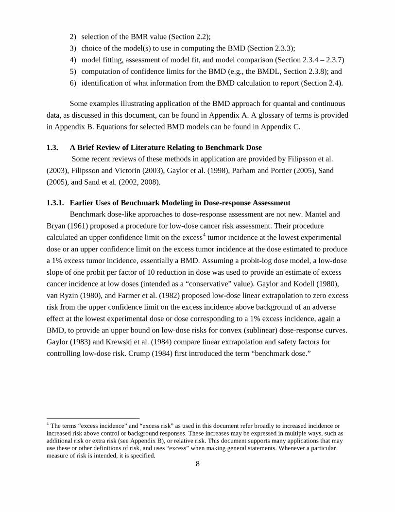
2) selection of the BMR value (Section 2.2); 3) choice of the model(s) to use in computing the BMD (Section 2.3.3); 4) model fitting, assessment of model fit, and model comparison (Section 2.3.4 – 2.3.7) 5) computation of confidence limits for the BMD (e.g., the BMDL, Section 2.3.8); and 6) identification of what information from the BMD calculation to report (Section 2.4).

Some examples illustrating application of the BMD approach for quantal and continuous data, as discussed in this document, can be found in Appendix A. A glossary of terms is provided in Appendix B. Equations for selected BMD models can be found in Appendix C. 1.3. A Brief Review of Literature Relating to Benchmark Dose Some recent reviews of these methods in application are provided by Filipsson et al. (2003), Filipsson and Victorin (2003), Gaylor et al. (1998), Parham and Portier (2005), Sand (2005), and Sand et al. (2002, 2008). 1.3.1. Earlier Uses of Benchmark Modeling in Dose-response Assessment Benchmark dose-like approaches to dose-response assessment are not new. Mantel and Bryan (1961) proposed a procedure for low-dose cancer risk assessment. Their procedure calculated an upper confidence limit on the excess4

tumor incidence at the lowest experimental dose or an upper confidence limit on the excess tumor incidence at the dose estimated to produce a 1% excess tumor incidence, essentially a BMD. Assuming a probit-log dose model, a low-dose slope of one probit per factor of 10 reduction in dose was used to provide an estimate of excess cancer incidence at low doses (intended as a “conservative” value). Gaylor and Kodell (1980), van Ryzin (1980), and Farmer et al. (1982) proposed low-dose linear extrapolation to zero excess risk from the upper confidence limit on the excess incidence above background of an adverse effect at the lowest experimental dose or dose corresponding to a 1% excess incidence, again a BMD, to provide an upper bound on low-dose risks for convex (sublinear) dose-response curves. Gaylor (1983) and Krewski et al. (1984) compare linear extrapolation and safety factors for controlling low-dose risk. Crump (1984) first introduced the term “benchmark dose.”

4 The terms “excess incidence” and “excess risk” as used in this document refer broadly to increased incidence or increased risk above control or background responses. These increases may be expressed in multiple ways, such as additional risk or extra risk (see Appendix B), or relative risk. This document supports many applications that may use these or other definitions of risk, and uses “excess” when making general statements. Whenever a particular measure of risk is intended, it is specified.

9

1.3.2. Properties of the Benchmark Dose A number of research efforts have compared benchmark doses with NOAELs. Many of these have dealt with reproductive and developmental toxicity data, and have demonstrated effects of 10% and greater in terms of excess probability (dichotomous data) or change from control means (continuous data) at conventional NOAELs (e.g., Alexeeff et al. 1993; Catalano et al. 1993; Chen et al. 1991; Krewski and Zhu 1994, 1995; Auton 1994; Crump 1995; Fowles et al. 1999; Leisenring and Ryan 1992; Gaylor 1992). In a series of papers by Faustman et al. (1994), Allen et al. (1994a, b), and Kavlock et al. (1995), the BMD approach was applied to a large database of developmental toxicity studies (with approximately 20 litters per dose group). In brief, the results of these studies showed that when the data were expressed as the proportion of affected fetuses per litter (nested dichotomous data), the NOAEL was on average 0.7 times the BMDL for a 10% excess probability of response and was approximately equal, on average, to the BMDL for a 5% excess probability of response. When data were expressed as counts of dichotomous endpoints (i.e., number of litters per dose group with resorptions or malformations), the NOAEL was approximately 2–3 times higher than the BMDL for a 10% probability of response above control values and 4–6 times higher than the BMDL for a 5% excess probability of response. Expressing the data as the proportion of affected fetuses per litter is the more rigorous way to analyze developmental toxicity data. However, the results of the quantal data analysis also may apply to using the BMD approach with other quantal data and suggest that the NOAEL in these cases may be at or above the 10% true excess response level, depending on sample size and background rate. Since reduced fetal weight in developmental toxicity studies often shows the lowest NOAEL among the various endpoints evaluated, the application of the BMD approach to these continuous data also was evaluated (Kavlock et al. 1995). A variety of cutoff values was explored for defining an adverse level of weight reduction below control values. In some cases, data were analyzed using a continuous power model, and in other cases, the data were transformed to dichotomous data. Comparisons with the NOAEL showed that several cutoff values gave BMDL values similar to the NOAEL. These analyses suggest ways in which BMDs may be developed for continuous data from a variety of endpoints. Fowles et al. (1999) examined acute inhalation lethality data and compared NOAELs to BMDLs corresponding to 1%, 5%, and 10% excess response incidences. Sample sizes averaged from 10 to 20 animals per dose group. Similarly to the “quantal” parts of the results of the Allen et al. (1994a, b) studies, BMDLs based on 10% excess incidence corresponded approximately to NOAELs. However, because the dose-response relationship for these lethality data was so steep, BMDLs for 5% and 1% excess incidences were very close to those for 10% excess incidence. As

10

a result, the BMDLs for a 1% excess incidence were on average only about 1.6 or 3.6 times smaller than a NOAEL, depending on whether a log-probit or Weibull model was used. In addition to these comparisons with NOAELs, a simulation study by Kavlock et al. (1996) examined BMDL in relation to various aspects of study design (number of dose groups, dose spacing, dose placement, and sample size per dose group) for two endpoints of developmental toxicity (incidence of malformations and reduced fetal weight). Of the designs evaluated, the best results (that is, those with the narrowest confidence intervals) were obtained when two dose levels had response rates above the background level, one of which was near the BMR. In this study, there was virtually no advantage in increasing the sample size from 10 to 20 litters per dose group. When neither of the two dose groups with response rates above the background level was near the BMR, satisfactory results were also obtained, but the BMDLs tended to be lower. When only one dose level with a response rate above background was present and near the BMR, reasonable results for the maximum likelihood estimate and BMDL were obtained, but in this case, there were benefits of larger dose group sizes. The poorest results were obtained when only a single group with an elevated response rate was present and the response rate was much greater than the BMR. 1.3.3. Approaches to BMD Computation Many noncancer health effects are characterized by multiple endpoints that are not completely independent of one another. Lefkopoulou et al. (1989), Chen et al. (1991), Ryan (1992a, b), Catalano et al. (1993), Zhu et al. (1994), Krewski and Zhu (1995), and Fung et al. (1998) have worked on this issue using developmental toxicity data and have shown that, in most cases, the BMDL derived from a multinomial modeling approach is lower than that for any individual endpoint. This approach has not been applied to other health effects data but should be kept in mind when multiple related outcomes are being considered for a particular health effect. Dose-response modeling of continuous endpoints for risk assessment is made more difficult because there is not a natural probability scale with which to characterize risk. The challenge is in re-interpreting effects on a continuous scale so that the result may be thought of in terms of risk, as is done for quantal endpoints. One approach is to explicitly dichotomize such continuous endpoints and then model the explicitly dichotomized endpoints as any other quantal endpoint. In separate papers, Crump (1995) and Kodell et al. (1995) detailed an approach to deriving BMDs for continuous data based on a method originally proposed by Gaylor and Slikker (1990). This approach, frequently called the “hybrid” approach, makes use of the distribution of continuous data, estimates the incidence of individuals falling above or below a level considered to be adverse or at least abnormal, and gives the probability of responses at specified doses above the control levels. The result is an expression of the data in the same terms as that derived from analyses of quantal data. That is, the approach implicitly dichotomizes the

11

data, retaining the full power of modeling the continuous data while obtaining results that permit direct comparison of BMDs and BMDLs derived from continuous and quantal data. Gaylor (1996) compared BMDs computed for continuous endpoints directly to those computed after first explicitly dichotomizing the data and found that, even for moderate sample sizes, substantial precision was lost upon explicitly dichotomizing the data. West and Kodell (1999) compared such an implicit method for continuous data to the result of modeling explicitly dichotomized endpoints. For sample sizes in the range of 10 to 20 animals per dose group, West and Kodell found that the implicit approach gave substantially better results than did the approach of modeling explicitly dichotomized data. Thus, when possible, it is generally better to derive BMDs and BMDLs for continuous data from models of the continuous data, perhaps using the hybrid approach described by Gaylor and Slikker (1990), Crump (1995), or Kodell et al. (1995). Crump (2002) discusses current, unresolved issues in BMD calculation for continuous data. Most approaches to BMD modeling have focused on modeling single or multiple responses from a single study. Categorical regression modeling (Dourson et al. 1985; Hertzberg 1989; Hertzberg and Miller 1985; Guth et al. 1997; Simpson et al. 1996a, b) is one method that allows the results for multiple endpoints across studies to be used to make an overall assessment of the toxicity of a compound based on a larger database. Although so far this method has not been widely used for BMD computation, it shows promise as a way to more quantitatively and rigorously combine information from a rich database. Bayesian approaches to BMD calculation express the uncertainty in the BMD estimate with a probability distribution (in Bayesian parlance, the posterior distribution), in contrast to the confidence limits employed by the more commonly used frequentist approach (Hasselblad and Jarabek 1995). Although the Bayesian approach has not yet found wide application, it has some potentially useful features. The Bayesian approach facilitates combining results from different datasets to provide a more robust estimate as well as an evaluation of the uncertainty in that estimate that would take into account the variability among studies. This type of approach may lead to improvements over the more widely used methods, which only quantify the uncertainty inherent in a single study. Gaylor et al. (1998) reviewed statistical methods for computing BMDs, and Murrell et al. (1998) discussed some consequences of using the confidence limits on BMDs as PODs and suggested an approach for setting BMR levels for continuous endpoints. 1.3.4. Historical Development of this Benchmark Dose Technical Guidance Several workshops and symposia have been held to discuss the application of the BMD methodology (Kimmel et al. 1989; California EPA 1994; Beck et al. 1993; Barnes et al. 1995; U.S. EPA 1996b). On the whole, the participants at the 1995 U.S. EPA co-sponsored workshop (Barnes et al. 1995) endorsed the application of the BMD approach for all quantal noncancer

12

endpoints and particularly for developmental toxicity, where a good deal of research has been done. Less information was available at the time of the workshop on the application of the BMD approach to continuous data, and more work was encouraged. These workshops and discussions informed the development of an earlier draft of this document, which was released for public and scientific peer review in 2000. The guidance and recommended options set forth in this final document are based largely on the 2000 draft, on the comments of the external peer review panel, and on experience gained from application of the methodology in U.S. EPA risk assessments.

2. BENCHMARK DOSE GUIDANCE This section describes the proposed approach for carrying out a complete BMD analysis. It is organized in the form of a decision process, including the rationales and recommended defaults for proceeding through the analysis. The guidance suggests some constraints on the BMD analysis through decision criteria and proposes defaults when more than one feasible approach exists. 2.1. Data Evaluation The first step in the process of hazard characterization is a complete review of the toxicity data available about an agent in order to identify and characterize the hazards related to a particular compound or exposure situation. This involves determining the adverse effects or precursors of adverse effects from all available data and the most relevant endpoints on which to base NOAELs or BMDs. Guidance on review of endpoint data for hazard characterization can be found in a number of U.S. EPA publications focused on carcinogenicity, developmental toxicity, neurotoxicity, and other health effects (U.S. EPA 1991, 1996a, 1998, 2005a). This process is essentially the same whether using a BMD or a NOAEL approach. The following discussion summarizes some of the more important issues related to study design and data reporting when using the BMD approach. Some of the decision-making steps associated with data evaluation and discussed in this Section are summarized in the flowchart in Figure 2A (Section 2.1.5). This guidance does not change the way in which hazard characterization is done, particularly regarding the determination of adversity and selection of endpoints. This guidance does discuss the types of data and study designs most amenable to dose-response modeling, and it allows for the possibility that NOAELs/LOAELs will continue to be used for some datasets. Resorting to the NOAEL/LOAEL approach does not resolve a data set’s inherent limitations, but it conveys that there are limitations with the data set.

13

2.1.1. Study Design In general, studies with more dose groups and a graded monotonic response with dose will be more useful for BMD analysis. Studies with only a single dose showing a response different from controls may not support BMD analysis, though if the one elevated response is near the BMR, adequate BMD and BMDL computation may result (Kavlock et al. 1996). Studies in which responses are only at the same level as background or at or near the maximal response level are not considered adequate for BMD analysis. (See Section 2.1.5 for more discussion.) It is preferable to have studies with one or more doses near the level of the BMR to give a better estimate of the BMD. 2.1.2. Aspects of Data Reporting In many cases, the risk assessor must rely on summary reports of key toxicological studies, which can vary in completeness vis-a-vis the data requirements of the BMD method. The optimal situation is to have information on individual subjects, but this is unlikely in the peer-reviewed literature. It is more common to have summary information (group level information, e.g., mean and SD) concerning the measured effect, especially for continuous response variables, and it must be determined whether the summary information is adequate for the BMD method to be applied. Dichotomous (or quantal) data are normally reported at the individual level (e.g., 11/50 animals showed the effect). Occasionally, a dichotomous endpoint will be reported as being observed in a group with no mention of the number of animals showing the effect. This usually occurs when the incidence of the endpoint reported is ancillary to the focus of the report. For BMD modeling of dichotomous data, both the number showing the response and the total number of subjects in the group are necessary. Continuous data are reported as a measurement of the effect, such as body weights or enzyme activity, in control and exposed groups. The response might be reported in several different ways, e.g., as an actual measurement or as a contrast—relative change from control. To model continuous data when individual animal data are not available, the number of subjects, mean of the response variable, and a measure of variability (e.g., SD; standard error (SE); or variance) are needed for each group. The lack of a numerically reported SD or SE may preclude the calculation of a BMD. In some cases, a measure of variability is presented for the control group only and this information might be used for modeling by making an assumption, for example, that the variance in the exposed groups is the same as in the controls. However, this assumption may not be correct, and the modeling of the data and calculation of the confidence limits will not be as reliable or precise as when the variance information is available for individual groups. Categorical data are data in which more than one defined category exists in addition to the no-effect category (responses within categories are quantal). When observations in the

14

treatment groups are characterized in terms of the severity of effect (e.g., mild, moderate, or severe histological change), these are ordered categorical data (also called ordinal data). Results may be classified by reporting an entire treatment group in terms of category (group level reporting) or by reporting the number of animals from each group in each category (individual level reporting). For example, a report of epithelial degenerative lesions might state that an exposed group showed a mild effect (group level) or that in the exposed group there were seven animals with a mild effect and three with no effect (individual level reporting). In the latter case, the BMD can be calculated using a quantal model after combining data in severity categories (e.g., model all animals with greater than a mild effect). Dichotomous data can be viewed as a special case in which there is one effect category and the possible response is binary (e.g., effect or no effect). Modeling approaches have been discussed for categorical data with multiple categories (Dourson et al. 1985; Hertzberg 1989; Hertzberg and Miller 1985) and for group level categorical data (Guth et al. 1997; Simpson et al. 1996a, b). These models can also be used to derive a BMD by estimating the probability of effects of different levels of severity. In addition, as for data evaluation in general, data (responses and doses) should be validated to the extent possible. For example, the original source should be examined, if possible, and any deliberate omissions of dose groups or subjects by the authors should be recognized and their basis understood. The suitability of control conditions will need to be assessed; if two types of control groups are available for the analysis, the most appropriate one is generally selected (e.g., the vehicle control). 2.1.3. Selection of Studies to be Modeled Following a complete review of the toxicity data, the risk assessor selects the studies for BMD analysis, based on the human exposure situation being addressed, the quality of the studies, the reporting adequacy, and the relevance of the endpoints. The process of selecting studies for BMD analysis is intended to identify those studies for which modeling is feasible, so that BMDs can be calculated. All relevant studies should be considered for modeling. In some cases, the selection process will identify a single study or very few studies for which calculations are appropriate. In other cases, there may be a number of studies, or studies with a number of endpoints reported, which may require a large number of BMD calculations. In these latter cases, it may be possible to select a subset of endpoints as representative of the effects in a target organ or study. This selection can be made on the basis of sensitivity or severity, which may be more easily compared within a single study in the same target organ than across studies. Sometimes combining several datasets may be an option (see Section 2.1.6 for more discussion). 2.1.4. Selection of Endpoints to be Modeled Once studies have been evaluated with regard to their feasibility for BMD modeling, the selection of endpoints to model should focus on the dose-response relationships. Typically, all

15

endpoints within a study that the risk assessor has judged to be relevant to the exposure should be considered for modeling. This will help ensure that no endpoints with the potential of having the most sensitive effect for risk assessment applications, usually having the lowest BMDL, are excluded from the analysis. The apparent relative sensitivities of endpoints based on NOAELs/LOAELs may not correspond to the same relative sensitivities based on BMDs or BMDLs after BMD modeling; therefore, relative sensitivities of endpoints cannot necessarily be judged a priori. For example, differences in slope (at the BMR) among endpoints could affect the relative values of the BMDLs. Selected endpoints from different studies that have the potential to be used in the determination of a POD(s) should all be modeled, especially if different UFs may be used for different studies and endpoints. The risk assessor selects the BMDL(s) to serve as the POD(s) using scientific judgment and principles of risk assessment as well as the results of the modeling process. Note that it is sometimes desirable to carry through risk estimate derivations for multiple endpoints for comparisons and other purposes. 2.1.5. Minimum Dataset for Calculating a BMD Once the critical endpoints have been selected, datasets are examined for the feasibility of a BMD analysis. Recommended minimum dataset criteria for BMD modeling, summarized in Figure 2A and 2B, include the following:

• There should be at least a statistically or biologically significant dose-related trend in the selected endpoint.5

• The dataset should contain information on the dose-response relationship between the extremes of the control level and the maximal response observed. An ideal situation is to have (a) datapoint(s) near the BMR. The following examples illustrate cases that may fail to satisfy this minimum dataset criterion:

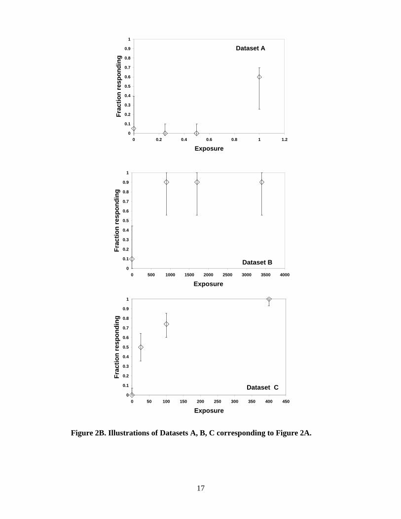
o A dataset with only the highest dose showing a response (e.g., Dataset A in Figure 2B) would bracket the BMD at the low end but may provide limited information about the shape of the dose-response relationship. In such cases, dose spacing and the proximity of the BMR to the observed response level will influence the uncertainty in the BMD estimate. Fitting multiple models to the dataset will help evaluate the magnitude of this uncertainty. The modeling exercise itself may provide insight on the degree of uncertainty associated with an estimated BMD.

o A dataset in which all non-control doses have essentially the same response level (e.g., Dataset B in Figure 2B) provides limited information about the dose-response relationship since the complete range of response from background to maximum must occur somewhere below the lowest dose; thus, the BMD may be just below the first dose, or orders of magnitude lower. When this situation arises, it is tempting to use a model such as the Weibull with no restrictions on the power parameter (in quantal data, especially if the maximal response is less than 100%); however, this can result in models that are improbably steep in the low-dose region (see Section 2.3.3.3.). The unfortunate reality in such situations is that the data provide little useful information

5 In some cases biological significance may be inferred from other data on the same chemical and endpoint.

16

about the dose-response relationship at lower doses; the ideal solution is to collect further data in the dose range missed by the studies in hand.

Figure 2A. Flowchart of data evaluation steps for determining BMD modeling feasibility. (See Figure 2B for Datasets A, B, and C.)

no

Is there a biologically or statistically significant trend?

Statistical significance not required - monotonic trend in rare endpoints, or adverse endpoints in studies with low power may be biologically significant.

Are there enough dose groups?

Too few groups generally limits the number of applicable models:• One group usually not enough, but if it is in useful range of exposure/response, modeling can provide estimate of response and confidence limits• Two groups may support a model fit, but may not help evaluate model uncertainty in final result• Number of groups should be at least as large as the number of model parameters to estimate mean responses and confidence intervals.

Example: If using mean responses, are there standard deviations or errors?

Examples: • If survival or timing of response is an issue, are enough data available to address it?• If developmental effects, are fetal data provided within litters?

Data partly incomplete - proceed cautiously with modeling; reported estimates may incorporate more uncertainty than with complete data

yes

no

maybe

yes

yes

STOP: Cannot model or assess NOAEL/LOAEL from these data.Is there another endpoint or dataset?

no

NOAEL/LOAEL Include confidenceintervals on response levels

Every non-zero dose has the same response (Dataset B). If quantal data is the response well below 100%?

Is the dose-response relationship amenable to modeling?

Clear dose-response, but lowest dose has a high response (Dataset C) relative to BMR. Model?

Only response seen is at high dose (Dataset A). If quantal data, is the response well below 100%?

Are there adequate model fits and estimates of BMDsand BMDLs?

In addition to fitting models to all data points, consider fitting a model approximating a straight line between adjacent doses with different response levels.

maybeyes

Examples:• Is there a clear dose-response relationship, with overall monotonic changes with increasing dose level (taking biological considerations into account)?• Are the data extremely sublinear or supralinear?• Is desired BMR near range of observed responses?

Modeling often “works,”but may also be uninformative. . .

no

or maybe

or maybe

yes

Especially consider model uncertainty for extrapolating to lower doses/ responses than observed

Move on to next phase of analysis

no

no

no

yesyes

yes

Are there sufficient data?

Is there another dataset with lower exposures?

consider

consider

no

Is there a biologically or statistically significant trend?

Statistical significance not required - monotonic trend in rare endpoints, or adverse endpoints in studies with low power may be biologically significant.

Are there enough dose groups?

Too few groups generally limits the number of applicable models:• One group usually not enough, but if it is in useful range of exposure/response, modeling can provide estimate of response and confidence limits• Two groups may support a model fit, but may not help evaluate model uncertainty in final result• Number of groups should be at least as large as the number of model parameters to estimate mean responses and confidence intervals.

Example: If using mean responses, are there standard deviations or errors?

Examples: • If survival or timing of response is an issue, are enough data available to address it?• If developmental effects, are fetal data provided within litters?

Data partly incomplete - proceed cautiously with modeling; reported estimates may incorporate more uncertainty than with complete data

yes

no

maybe

yes

yes

STOP: Cannot model or assess NOAEL/LOAEL from these data.Is there another endpoint or dataset?

no

NOAEL/LOAEL Include confidenceintervals on response levels

Every non-zero dose has the same response (Dataset B). If quantal data is the response well below 100%?

Is the dose-response relationship amenable to modeling?

Clear dose-response, but lowest dose has a high response (Dataset C) relative to BMR. Model?

Only response seen is at high dose (Dataset A). If quantal data, is the response well below 100%?

Are there adequate model fits and estimates of BMDsand BMDLs?

In addition to fitting models to all data points, consider fitting a model approximating a straight line between adjacent doses with different response levels.

maybeyes

Examples:• Is there a clear dose-response relationship, with overall monotonic changes with increasing dose level (taking biological considerations into account)?• Are the data extremely sublinear or supralinear?• Is desired BMR near range of observed responses?

Modeling often “works,”but may also be uninformative. . .

no

or maybe

or maybe

yes

Especially consider model uncertainty for extrapolating to lower doses/ responses than observed

Move on to next phase of analysis

no

no

no

yesyes

yes

Are there sufficient data?

Is there another dataset with lower exposures?

considerconsider

consider

17

0

0.1

0.2

0.3

0.4

0.5

0.6

0.7

0.8

0.9

1

0 0.2 0.4 0.6 0.8 1 1.2

Exposure

Frac

tion

resp

ondi

ng

Dataset A

0

0.1

0.2

0.3

0.4

0.5

0.6

0.7

0.8

0.9

1

0 500 1000 1500 2000 2500 3000 3500 4000

Exposure

Frac

tion

resp

ondi

ng

Dataset B

0

0.1

0.2

0.3

0.4

0.5

0.6

0.7

0.8

0.9

1

0 50 100 150 200 250 300 350 400 450

Exposure

Frac

tion

resp

ondi

ng

Dataset C

Figure 2B. Illustrations of Datasets A, B, C corresponding to Figure 2A.

18

o A variation of the above example is a dataset in which the non-control doses do not necessarily all have the same response level but, nonetheless, the first non-control dose has a response level substantially above the selected BMR (e.g., Dataset C in Figure 2B). Depending on the dataset, the BMD may, as above, be just below the first dose or considerably lower. Sometimes in such cases, information provided by the higher doses in the dataset can reduce uncertainty about the shape of the dose-response relationship near the first dose. Fitting multiple models to the dataset will help evaluate the magnitude of model uncertainty in the BMD estimate.

o When there is a jump between no response and maximal (or near-maximal) response between two non-control doses, there is still limited information about the dose-response relationship, but the dose spacing may ameliorate the situation since the BMD is effectively bracketed between the two doses that determine the jump. Case-by-case judgments will have to be made based on the dose spacing to determine if modeling can be used. The modeling exercise itself may provide insight on the degree of uncertainty associated with an estimated BMD.

2.1.6. Combining Data for a BMD Calculation Datasets that are statistically and biologically compatible may be combined prior to dose-response modeling, resulting in increased confidence, both statistical and biological, in the calculated BMD. The simplest approach to combining datasets is to treat the data as if they were all collected simultaneously. If it is plausible that the multiple datasets represent a homogeneous picture of the dose-response (for example, the responses at doses common to two or more datasets are essentially the same and statistically undifferentiable), then this is a justifiable approach.

Allen et al. (1996) provided an example of a case where data on boron-associated developmental effects could be combined for the BMD analysis, based on an evaluation of log likelihoods. Another example is provided in U.S. EPA's assessment of the dominant lethal effects of 1,3-butadiene, in which data from three different studies conducted by the same laboratory were combined (U.S. EPA 2002b, Section 10.3.3). More likely, there will be some variability among datasets, requiring more elaborate modeling to combine information properly. There is as yet too little practical, as well as theoretical, experience with this situation to provide specific guidance in the matter, other than to say that statistically appropriate methods and biological judgment must be used and justified if datasets are combined for modeling. One technique for statistically accommodating variability among studies is categorical regression analysis (Simpson et al. 1996a, b), although this method requires a large number of studies for the chemical of interest. Examples of accommodating variability while combining datasets to estimate a BMD for a single endpoint are presented in U.S. EPA's cumulative risk assessments for organophosphate and n-methyl carbamate pesticides (U.S. EPA 2002c, 2005b).

19

2.1.7. Dosimetric Adjustments Often dosimetric adjustments are used to convert the doses administered to experimental animals into lifetime continuous human-equivalent doses (HEDs, e.g., U.S. EPA 1994, 2002a, 2011). While it is beyond the scope of this document to provide guidance for deriving or applying these adjustments, this section notes some general circumstances in which dosimetric adjustments may be important to consider prior to dose-response modeling.

It is generally preferable to model the experimental animal response data with experimental animal doses (e.g., applied dose, internal dose metric), in order to describe the dose-response relationship before any assumptions about interspecies extrapolation are invoked. If the adjustment is proportional across the doses (e.g., a constant adjustment for continuous exposure), then whether one adjusts the doses before or after the modeling does not affect the end results and is more a matter of convenience. If, however, the adjustments are not proportional across the doses, then it may be more suitable to make the dosimetric adjustments before the dose-response modeling. This could be the case, for example, when the available data only support interspecies scaling through body weight scaled to the ¾-power and the body weights differ notably across dose groups. Similarly, physiologically based pharmacokinetic (PBPK) modeling often reflects processes that are nonlinear with dose. When PBPK model-derived dose metrics are available, multiple options may merit consideration. Nonlinear curve fitting using the experimental exposure doses/concentrations can be used to estimate the BMD/BMDL, which can then be converted to the human equivalent values or to the levels of a pertinent dose metric (e.g., area under the curve [AUC] of metabolite concentration in the liver) using an experimental animal PBPK model. For highly supralinear dose-response relationships there may be difficulties adequately fitting a curve using applied doses, so it may be advantageous to use an internal dose metric for the dose-response modeling. If an internal dose metric from an experimental animal PBPK model is used, the HEDs for the BMD and BMDL would be back-calculated through a human PBPK model or estimated in some other way. Dose-response analyses in terms of an internal dose metric may simplify the dose-response relationship (e.g., linearize a supralinear curve due to metabolic saturation), potentially improving curve fitting, and may help elucidate the contributions of the pharmacokinetic processes versus the pharmacodynamic processes to the observed dose-response relationship. 2.2. Selection of the Benchmark Response Level (BMR) Selecting a BMR(s) involves making judgments about the statistical and biological characteristics of the dataset and about the applications for which the resulting BMDs/BMDLs will be used. The EPA does not currently have guidance to assist in making such judgments for the selection of the response levels, or BMRs, to use with BMD modeling for most applications (e.g., for calculating reference doses or relative potency factors), and such guidance is beyond

20

the scope of this document. U.S. EPA's Guidelines for Carcinogen Risk Assessment (U.S. EPA 2005a) address BMRs for cancer risk estimation. This section outlines some general principles to consider, along with case-specific issues, as well as BMRs for standard reporting, i.e., to facilitate comparisons across chemicals or endpoints. Typically, a BMR near the low end of the observable range is selected as the basis for obtaining BMDs and BMDLs to serve as potential PODs for deriving quantitative estimates below the range of observation and to use for comparisons of effective doses corresponding to a common response level across chemicals, studies, or endpoints. Because different study designs have different dose selections and different sensitivities (i.e., statistical power) to observe adverse effects at various doses, the low end of the observations can correspond to disparate response levels across studies. It is important to recognize that the BMR need not correspond to a response that the study could detect as statistically significantly different from the control response, provided that the response is considered biologically significant.

For some datasets the observations may correspond to response levels far in excess of a selected BMR and extrapolation sufficiently below the observable range may be too uncertain to reliably estimate BMDs/BMDLs for the selected BMR (e.g., when all the dosed groups have near-maximal responses). In such cases, BMD modeling is not recommended6

The following describes options used for selecting the BMR. For quantal (dichotomous) data, the conventional approaches are fairly straightforward. For continuous data, on the other hand, there is less historical precedence upon which to draw; however, some reasonable options are presented. The rationale supporting each selected BMR should be provided. Once a BMR is selected and the dose-response data are modeled, the BMD is explicitly determined.

and obtaining more data or using the NOAEL/LOAEL approach, while recognizing the inabilities of that approach to resolve the data limitations, may be warranted (see Section 2.1.5.).

2.2.1. Quantal (Dichotomous) Data

As mentioned above, there are several applications for BMDs/BMDLs, requiring separate decisions for selecting BMRs. For comparing potencies across chemicals or endpoints (e.g., for chemical rankings) for dichotomous data, a response level of 10% extra risk has been commonly used to define BMDs, also known as effective doses (i.e., ED10s). This response level is used for such comparisons because it is near the low end of the observable range for many common study designs. In general, it is recommended that comparisons across chemicals/studies/endpoints be based on central estimates; this is in contrast to using lower bounds for PODs for reference values or cancer potency estimates.

6 A detailed decision process is not provided because of varying characteristics of datasets to be modeled, and because relevant information, such as mode of action, may be influential. The decision not to rely on BMD modeling should be made case by case, by statisticians or others trained in modeling and by scientists familiar with the type of data under consideration or with the particular database.

21

For the determination of a POD, however, it is not always critical that a common response level be used for all chemicals or endpoints, and for the purposes of deriving quantitative estimates at doses below the observable range, it may be desirable to use response levels other than 10% extra risk, if supported by the statistical and biological characteristics of the data set. In addition, for epidemiological data, response rates of 10% extra risk would often involve upward extrapolation, in which case it is desirable to use lower levels, and 1% extra risk is often used as a BMR. Providing guidance for the judgments involved in weighing the biological (e.g., nature of the endpoint, including mode of action) and statistical (e.g., study sensitivity) considerations in BMR selection is beyond the scope of this document. Nonetheless, for transparency, a justification should be provided for each BMR selection, addressing these considerations. Thus, while it is important always to report BMDs (and BMDLs) corresponding to 10% extra risk for comparison purposes, the BMD (BMDL) used as a POD may correspond to response levels below (or sometimes above) 10% extra risk. For standardization, rounded levels of 1%, 5%, or 10% have typically been used. In summary:

• An extra risk of 10% is recommended as a standard reporting level for quantal data, for the purposes of making comparisons across chemicals or endpoints. The 10% response level has customarily been used for comparisons because it is at or near the limit of sensitivity in most cancer bioassays and in noncancer bioassays of comparable size. Note that this level is not a default BMR for developing PODs or for other purposes.

• Biological considerations may warrant the use of a BMR of 5% or lower for some types of effects (e.g., frank effects), or a BMR greater than 10% (e.g., for early precursor effects) as the basis of a POD for a reference value.

• Sometimes, a BMR lower than 10% (based on biological considerations), falls within the observable range. From a statistical standpoint, most reproductive and developmental studies with nested study designs easily support a BMR of 5%. Similarly, a BMR of 1% has typically been used for quantal human data from epidemiology studies. In other cases, if one models below the observable range, one needs to be mindful that the degree of uncertainty in the estimates increases. In such cases, the BMD and BMDL can be compared for excessive divergence. In addition, model uncertainty increases below the range of data.

2.2.2. Continuous Data For continuous data, there are various possibilities for selecting the BMR. Regardless of which option is used, it is recommended that the BMD (and BMDL) corresponding to a change in the mean response equal to one control SD from the control mean always be presented for comparison purposes. This value would serve as a standardized basis for comparison, akin to the BMD corresponding to 10% extra risk for dichotomous data.

22

The ideal is to have a biological basis for the BMR for continuous data, e.g., a consensus scientific definition of what minimal level of change in a continuous endpoint is biologically significant. When there is a biological basis for BMR selection, the modeler has a choice of fitting a continuous model and using this defined level of change as a BMR or of “dichotomizing” the data on the basis of that level of change and fitting a quantal model. (See Section 2.3.3.1 below.) The latter approach results in a loss of information but may be useful when available continuous models are inadequate for the data. For example, if a 10% change in adult body weight is considered biologically significant, then a continuous model (with a BMR of 10% change) would provide a BMD corresponding to an average 10% weight change. Dichotomizing the data would involve summarizing the individual weight change data as incidences of subjects with a weight change of ≥10%. Then one must still define a BMR associated with an important change in incidence, say 10% extra risk. A quantal model is then used to estimate a BMD corresponding to a 10% extra risk of subjects having weight changes of at least 10%. However, in that case, the information about average weight change associated with the BMD is not available. In the absence of a sufficient biological basis to establish a cut-point for biological significance, one may have reason to dichotomize the data based on a percentile of the control distribution (e.g., Kavlock et al. 1995). Another approach is the “hybrid” approach, which fits continuous models to continuous data but expresses the BMD in terms used for quantal data (e.g., extra risk). As with dichotomizing the data, more than one cut-point must be defined. See Section 2.3.3.1 for more information about implementing hybrid models. Alternatively, in the absence of any cogent basis for selecting a BMR for continuous data, a BMR of one control SD (or lower or higher, if warranted by statistical and biological considerations7

7 Such as, whether the available data support extrapolation through consideration of study design, mode of action, etc.)

) change from the control mean can be used, as is recommended as the standardized reporting level for comparisons for continuous data. The control SD can be computed with the inclusion of historical control data, but the control mean should generally be from data concurrent with the treatments being considered (Crump 1995). If it can be estimated separately, the SD among animals apart from the SD due to measurement error should be used (Gaylor and Slikker 2004). Typically, however, only the overall SD, including measurement error, will be available. According to Gaylor and Slikker (2004), use of the overall SD results in an overestimation of the BMD; however, the bias is relatively small if the SD of measurement errors is less than one-third of the SD among animals, a condition the authors suggest is achieved in most experimental designs.

23

A one SD shift in the control mean corresponds to an extra risk of 10% for the proportion of individuals below the 1.4th percentile or above the 98.6th percentile of controls for normally distributed effects.8

(See Figure 3 for an illustration.) While a one SD change is the

Figure 3. Difference in population tail probabilities resulting from a one standard deviation shift in the mean from a standard normal distribution, illustrating the theoretical basis for a baseline BMR of 1 SD.

recommended BMR for comparisons across BMDs, this value may not always be suitable as a BMR for determining a POD. That is, a change of one SD in the control mean would be statistically significant in most studies with 10 or more animals per dose group, and the corresponding BMD would generally be interpreted as a LOAEL, depending, of course, on the biological significance of the outcome being measured. Thus, as previously discussed for quantal data, judgments about the biological and statistical characteristics of the data must be made. For example, for frank effects, a lower BMR may be warranted (e.g., 0.5 SD).

8 A one SD BMR is consistent with the observation of Crump (1995) that for a normal distribution with constant variance, 10% of a population exceeding the 1st or 99th percentile of the control distribution corresponds to a change in the mean of 1.1 times the SD.

0.00

0.05

0.10

0.15

0.20

0.25

0.30

0.35

0.40

0.45

0.50

-5.5 -5.0 -4.5 -4.0 -3.5 -3.0 -2.5 -2.0 -1.5 -1.0 -0.5 0.0 0.5 1.0 1.5 2.0 2.5

Prob

abili

ty

Standard deviation units

Control distribution

Distribution for group with mean response 1 SD below control mean

10% excessbelow controldistributionpercentile

1.4%-tile of control distribution

1 SD shift in mean

24

Without a biological basis or established scientific consensus (e.g., 10% change in body weight from the control mean) for selecting a BMR for continuous data, it is not recommended that a percent change in the control mean be used as the BMR because the same percent change for different endpoints (with different degrees of variability) could be associated with very different degrees of response. Sometimes the “dynamic range” has been used as a basis for defining the BMR. This involves scaling a continuous measurement by the range from the background response level to the maximum possible response level (Murrell et al. 1998) and selecting the BMR as a change in response scaled to the total response (e.g., 1% or 10%). This approach, however, requires a reliable estimate of the maximum achievable effect (Gaylor and Aylward 2004), and the toxicological relevance of some percent of the dynamic range is uncertain in situations where toxic effects at high exposures shift or differ qualitatively from those at low exposures. In addition, the comparability to other BMR definitions is not clear. Consequently the dynamic range approach is not currently recommended. A general hierarchy for BMR selection for continuous data is presented below. As noted above, a justification should always be provided for the selected BMR. For consistency in reporting, the BMD corresponding to a one control SD shift in the control mean should always be presented along with the BMDs and BMDL for whatever BMR is being used for the POD. In summary:

• Preferred approach: If there is a minimal level of change in the endpoint that is generally considered to be biologically significant, then that amount of change can be used to define the BMR.

• If individual data are available and a decision can be made about which individual levels can be reasonably considered adverse, then the data can be implicitly dichotomized using the hybrid model or explicitly dichotomized based on that cutoff value, and the BMR can be set as above for quantal data. Note that implicit dichotomization is preferred over explicit dichotomization, because of the loss of information associated with the latter.

• In the absence of any other idea of what level of response to consider adverse, a change in the mean equal to one control SD (or lower, e.g., 0.5 SD, for more severe effects) from the control mean should be used.

2.3. Modeling the Data 2.3.1. Introduction The goal of the mathematical modeling in BMD computation is to fit a model to dose-response data that describes the dataset, especially at the lower end of the observable dose-response range. The fitting must be done in a way that allows the uncertainty associated with parameter estimates to be quantified and related to the estimate of the dose that would yield the BMR. In practice, this procedure will involve first selecting a family or families of models for further consideration, based on characteristics of the data and experimental design, and fitting the

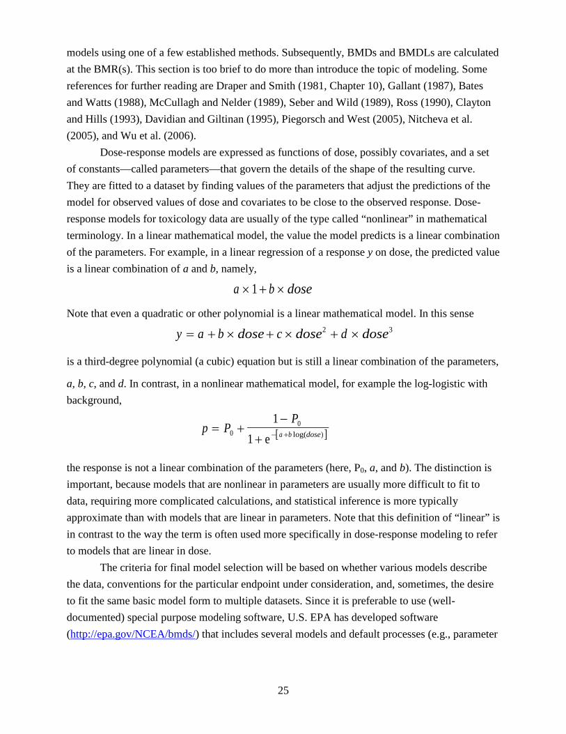
25

models using one of a few established methods. Subsequently, BMDs and BMDLs are calculated at the BMR(s). This section is too brief to do more than introduce the topic of modeling. Some references for further reading are Draper and Smith (1981, Chapter 10), Gallant (1987), Bates and Watts (1988), McCullagh and Nelder (1989), Seber and Wild (1989), Ross (1990), Clayton and Hills (1993), Davidian and Giltinan (1995), Piegorsch and West (2005), Nitcheva et al. (2005), and Wu et al. (2006). Dose-response models are expressed as functions of dose, possibly covariates, and a set of constants—called parameters—that govern the details of the shape of the resulting curve. They are fitted to a dataset by finding values of the parameters that adjust the predictions of the model for observed values of dose and covariates to be close to the observed response. Dose-response models for toxicology data are usually of the type called “nonlinear” in mathematical terminology. In a linear mathematical model, the value the model predicts is a linear combination of the parameters. For example, in a linear regression of a response y on dose, the predicted value is a linear combination of a and b, namely,

a b dose× + ×1

Note that even a quadratic or other polynomial is a linear mathematical model. In this sense

y a b dose c dose d dose= + × + × + ×2 3

is a third-degree polynomial (a cubic) equation but is still a linear combination of the parameters,

a, b, c, and d. In contrast, in a nonlinear mathematical model, for example the log-logistic with background,

[ ]p PP

a b dose= +−

+ − +001

1 e log( )

the response is not a linear combination of the parameters (here, P0, a, and b). The distinction is important, because models that are nonlinear in parameters are usually more difficult to fit to data, requiring more complicated calculations, and statistical inference is more typically approximate than with models that are linear in parameters. Note that this definition of “linear” is in contrast to the way the term is often used more specifically in dose-response modeling to refer to models that are linear in dose. The criteria for final model selection will be based on whether various models describe the data, conventions for the particular endpoint under consideration, and, sometimes, the desire to fit the same basic model form to multiple datasets. Since it is preferable to use (well-documented) special purpose modeling software, U.S. EPA has developed software (http://epa.gov/NCEA/bmds/) that includes several models and default processes (e.g., parameter

26

constraints) described in this document. For convenience, descriptions for the models mentioned in this document are provided in Appendix C. 2.3.2. Background for Model Selection The preference in selecting suitable models is to use those that are consistent with the biological processes understood to operate in a particular case and to avoid models that are clearly inconsistent. Characteristics that can be addressed in dose-response models include explicit expression of biologic processes (e.g., two-stage clonal expansion model developed by Moolgavkar and Knudson (1981) and Chen and Farland (1991); and saturable processes which may be characterized by Michaelis-Menten models) and key covariates of the responses under consideration (e.g., time of response in the multistage-Weibull model, pretreatment maternal body weight in nested models for developmental studies).

In the absence of a biologically based model, dose-response modeling is largely a curve-fitting exercise among the variety of available empirical models. Currently there is no recommended hierarchy of models that would expedite model selection, in part because of the many different types of datasets and study designs affecting dose-response patterns. As more flexible models are developed, hierarchies for some categories of endpoints will likely be more feasible. Some model hierarchies could be established as preferred practices. For example, it is a current practice of U.S. EPA’s IRIS program to prefer the multistage model for cancer dose-response modeling of cancer bioassay data (Gehlhaus et al., 2011). The multistage model (in fact a family of different stage polynomial models) is sufficiently flexible for most cancer bioassay data, and its use provides consistency across cancer dose-response analyses. This section provides some basic statistical background and guidance on choosing a model structure for the data being analyzed, fitting models, comparing models, and calculating confidence limits to derive a BMDL to use as a POD. 2.3.3. Selecting the Model The initial selection of a group of models to fit to the data is governed by the nature of the measurement that represents the endpoint of interest and the experimental design used to generate the data. In addition, certain constraints on the models or their parameter values sometimes need to be observed and may influence model selection. Finally, it may be desirable to model multiple endpoints at the same time. The diversity of possible endpoints and shapes of their dose-response relationships for different agents precludes specifying a small set of models to use for BMD computation. This will inevitably lead to the need for judgment when selecting the final model and BMD/BMDL for dose-response assessment. As experience using BMD methodology in dose-response assessment accumulates, it may be possible to narrow the number of models to a few that are sufficiently flexible and non-redundant to be specified for certain scenarios.

27

2.3.3.1. Type of endpoint The kind of measurement variable that represents the endpoint of interest is an important consideration in selecting mathematical models. Commonly, such variables are either continuous, like liver weight or the activity of a given liver enzyme, or dichotomous (quantal), like the presence or absence of abnormal liver status. However, other types occur in biological data; for example ordered categorical, like a histology score that ranges from 1-normal to 5-extremely abnormal. It is beyond the scope of this document to consider all possible kinds of variables that might be encountered, so further discussion will concentrate on dichotomous and continuous variables. Dichotomous variables. Data on dichotomous variables are commonly presented as a fraction or percent of individuals that exhibit the given condition at a given dose or exposure level. Note that for modeling dichotomous data, one uses the exact counts.9

Continuous variables. Data for continuous variables are often presented as means and SDs or SEs but may also be presented as a percent of control or some other standard. From a modeling standpoint, the most desirable form for such data is by individual. Unlike the usual situation for dichotomous variables, summarization of continuous variables results in a loss of information about the distribution of those variables. In addition, individual data is required when the intention is to use covariates in the analysis.

For such endpoints, normally we select probability density models like logistic, probit, Weibull, and so forth, with predictions between zero and one for any possible dose, including a zero dose.

The approach used to establish the BMR will determine the approach to modeling continuous data. (See Section 2.2.2 for more discussion.) Two broad categories of approach have been proposed:

1) If the BMR is defined as a level of change in a continuous endpoint (usually expressed as a particular change in the mean response, possibly as a fraction of the control mean, or as a fraction of the SD of the measurement from untreated individuals), a continuous model can be used. Typical continuous models include polynomial models, power models, and Hill models.

2) If the data are dichotomized and the BMR is defined as the proportion of individuals with more than a specified level of change in the continuous endpoint, the resulting variable can be modeled as dichotomous. Recall, however, that dichotomization results in a loss of information and should generally be avoided (Section 2.2.2).

An alternative is to use a hybrid approach, such as that described by Gaylor and Slikker

(1990), Kodell et al. (1995), and Crump (1995), which fits continuous models to continuous data, and, presuming a distribution of the data, calculates a BMD in terms of the fraction affected.

9 Note that survival-adjusted denominators may be used where relevant, e.g., via the poly-3 approach (Bailer and Portier, 1988), among others.

28

Using this approach, the probability (risk) of an individual with an adverse level can be estimated directly as a function of dose. The hybrid approach uses four steps, as summarized below. In the first step, the probability distribution of the continuous measure for individuals in the control group is characterized. Often this distribution may be approximately log-normal (i.e., the logarithms of the values of the biological measure are normally distributed). Since most biological effects do not assume negative values, the log-normal distribution satisfies this condition. If high values are adverse, a large percentile (e.g., 99th percentile) of the distribution may be selected as a cutoff value for normal levels, with larger values considered adverse. Conversely, if low values are adverse, a small percentile (e.g., 1st percentile) may be selected as a cut-off to classify individuals, with lower values considered adverse. In the second step, a dose-response model is fit to the data to establish how the average value changes as a function of dose. In the third step, the variability of individuals about the average values is calculated. Often this can be expressed simply by the SD about the average values. It is common for the SD of biological measurements to be proportional to their average value, i.e., a constant coefficient of variation. Again, this is a property of the log-normal distribution. However, the coefficient of variation may change with dose, which leads to a more complicated analysis of the data. In this case, it is often useful to model the variance as proportional to the mean raised to a power. Modeling the variance in this way can accommodate situations where the coefficient of variation is constant, where the variance is proportional to the square of the mean, and where the coefficient of variation is the square root of the constant of proportionality. (Example A.3 in Appendix A includes an illustration of variance modeling for a standard continuous model, the Hill model). From the average values estimated from the dose-response model in step 2 and the variability of values about the average values estimated in step 3, it is possible in the 4th step to estimate the probability, for any dose, that an individual is in the adverse range established in the first step. Hence, the BMD (and BMDL) can be estimated for a specified BMR. An example illustrating the use of each of the three techniques mentioned above can be found in the fetal weight analysis in U.S. EPA's 1,3-butadiene health assessment (U.S. EPA 2002b, Section 10.3.2). In this analysis, the continuous power model was used to model the average of mean fetal weights per litter as a continuous endpoint; the log-logistic model was used after dichotomizing the data, taking into account litter correlations; and the hybrid model was applied. 2.3.3.2. Experimental design The aspects of experimental design that bear on model selection include the total number of dose groups used and possible clustering of experimental subjects. The number of dose groups has a bearing on the number of parameters that can be estimated—the number of parameters that

29

affect the overall shape of the dose-response curve normally cannot exceed the number of dose groups. Clustering of experimental subjects is actually more of an issue for methods of fitting the models than for choice of the model form itself. The most common situation in which clustering occurs is in developmental toxicity experiments, where the agent is administered to the mothers and individual offspring within litters are examined for adverse effects. (See Appendix A, Example A.5.) Another example of clustering concerns designs in which individuals yield multiple observations (repeated measures). This can happen, for example, when each subject receives both treatment and control (common in studies with human subjects), or when each subject is observed multiple times after treatment (e.g., neurotoxicity studies). The issue in all these examples is that individual observations cannot be taken as independent of each other. Most methods used for fitting models rely heavily on the assumption that the data are independent, and special fitting methods need to be used for datasets that exhibit more complicated patterns of dependence. (See for example, Ryan 1992a, b; Davidian and Giltinan 1995.) Further details are beyond the scope of this document. 2.3.3.3. Constraints and covariates In dose-response modeling, the modeler may need to consider choices that constrain the set of parameter values that are numerically possible—typically for the purpose of strengthening the biological plausibility of the results. An obvious constraint on models for dichotomous data has already been discussed: probabilities are restricted to being positive numbers no greater than one. Biological realities impose other clear constraints on models. For example, most biological measures are positive; therefore, models should be selected so that their predicted values, at least in the region of application, conform to that constraint. Other choices have to do with the biological plausibility of dose-response patterns. For many toxic effects, a monotonic increase in effect with dose will be expected—that is, a higher dose will have an equal or greater effect than a lower dose. Thus, much existing practice has constrained models to be monotonic, for example in the fitting of the multistage model, the parameters are constrained to be nonnegative. In some circumstances non-monotonic relationships may be seen, most commonly when there are qualitatively altered biological mechanisms or observational limitations with high-dose data (see Section 2.3.6.)

Other questions arise with models that can be steeply supralinear for some parameter values. In models in which dose is raised to a power that is a parameter to be estimated (such as a Weibull model), the slope of the dose-response curve becomes very steep at low doses for power parameter values less than 1. This can raise difficult questions for the assessor. On the one hand, it is not uncommon for data in the observed range to show a supralinear response pattern (e.g.,

30

shape of Michaelis-Menten relationship), so excluding power parameters less than 1 may not provide the best fit to the data or allow adequate evaluation of uncertainty in response in the observed range. In principle, as BMD modeling does not generally seek to extrapolate to very low doses, the high slopes seen for some unconstrained models near the origin is not in itself a fundamental problem. On the other hand, in some instances, calculated BMDs and BMDLs can be very low when the power parameter is less than 1. This reflects the fact that the data do not constrain the lower end of the dose-response curve. For example, as noted earlier in this document, a particular problem arises with datasets where all non-control doses have response levels above the selected BMR and response is flat or shallow. When this situation arises with quantal data, especially if the maximum response is less than 100%, using a model like the Weibull with no restrictions on the power parameter is tempting because such models reach a plateau of less than 100% and most modeling programs do not include other models for quantal data that have this property. Using such an unconstrained model, however, can result in very imprecise BMDs because the data do not constrain the dose-response curve in this lower dose range, where all the change in response is occurring. In theory, other models could be found that force the BMD to be anywhere between the lowest BMDL and the lowest administered dose. Thus, the BMD computed here depends solely on the model selected, and goodness-of-fit provides no help in selecting among the possibilities. The unfortunate reality in such situations is that the data provide little useful information about the dose-response relationship; the ideal solution is to collect further data in the dose range missed by the studies in hand.

In general, the modeler should consider constraining power parameters to be 1 or greater (this is the default in the BMDS software;10

In quantal models, often a background parameter quantifies the probability that the outcome being modeled can occur in the absence of exposure. It may be tempting to reduce the number of parameters to be estimated by fixing the value of the background parameter to be zero. However, only when it is clear that an outcome would not occur in the absence of the exposure is it appropriate to fix the value of the background to zero.

see Example A.1). However, if the observed data do appear supralinear, unconstrained models or models that contain an asymptote term (e.g., a Hill model) warrant investigation to see whether they can support reasonable BMD and BMDL values. If they cannot, other model forms should be considered for a POD; at times, modeling will not yield useful results and the NOAEL/LOAEL approach might be considered, although the data gaps and inherent limitations of that approach should be acknowledged.

Inclusion of a so-called “threshold” term in the models is generally not recommended for BMD analysis. Although such a parameter is not an estimate of a biological threshold, it is easily mistaken for one due to confusing terminology. Furthermore, most datasets can be fit adequately 10 If such a parameter was constrained and was set to its constraint (= 1) during estimation, this fact should be reported. When this occurs, the nominal coverage of the confidence interval is not exact (asymptotically) and could be much less than intended if the true (unknown) parameter is <1, and this should also be reported.

31

without this parameter and the associated loss of a degree of freedom. However, on rare occasions, the increase in a response may be so precipitous that including a threshold parameter is needed for dose-response modeling with commonly available models, and in such cases including the parameter is acceptable. The inclusion of covariates on individuals is sometimes desirable when fitting dose-response models. For example, litter size has often been included as a covariate in modeling laboratory animal data in developmental toxicity studies. Another example is in modeling epidemiology data when certain covariates (e.g., age, parity) are included that are expected to affect the outcome and might be correlated with exposure. If the covariate has an effect on the response, including it in a model may improve the precision of the overall estimate by accounting for variation that would otherwise end up in the residual variance. Any variable that is correlated (non-causally) with dose and which affects outcome should be considered as a covariate.11

2.3.4. Model Fitting The goal of the fitting process is to find values for all the model parameters so that the resulting fitted model describes those data as well as possible; this is termed “parameter estimation.” One way to achieve this is to identify a function (the objective function) of all the parameters and all the data with the property that the parameter values that correspond to an overall minimum (or, equivalently, an overall maximum) of the function give the desired model predictions. The most common ways to construct and optimize objective functions include the methods of maximum likelihood, nonlinear least squares, and generalized estimating equations (GEE). The choice of objective function is determined in large part by the nature of the endpoint and of the variability of the data around the fitted model, so that at times only one method may be suitable for a data type. The methods are described further below, along with some limitations on their use with common data types:

• Dichotomous data—An example of such a situation is the case of individual independently treated animals (i.e., not clustered in litters) scored for the presence of a single response. Here it is reasonable to suppose that the number of responding animals follows a binomial distribution with the probability of response expressed as a function of dose.

• Continuous variables, especially means of several observations, are often normal (Gaussian) or log-normal. When variables are normally distributed with a constant variance, minimizing the sum of squares is equivalent to maximizing the likelihood, which explains in part why least squares methods, as discussed below, are often used for continuous variables.

11 Note that covariates define subsets of the study population, such as those in specific body weight ranges. Accordingly, different BMRs explicitly for different levels of the covariate(s) may be needed.

32

• In developmental toxicity data, the pregnant mother is the experimental unit and statistical methods must account for the tendency of littermates to respond similarly. The distribution of the number of animals with an adverse outcome is often taken to be approximately beta-binomial, in order to accommodate the lack of independence among littermates (litter effect; e.g., Chen and Kodell 1989; Williams 1975). One disadvantage of this method is a lack of robustness if the litter effect is modeled incorrectly (Kupper et al. 1986; Williams 1988). Alternative analyses can be based on quasi-likelihood, or more generally, generalized estimating equations, also discussed below. A simple approach using a simple data transformation has been described by Rao and Scott (1992) and Krewski and Zhu (1995) and has been shown to be as efficient as either the GEE or the maximum likelihood approach (Fung et al. 1998).

Maximum likelihood is a general way of deriving an objective function when a

reasonable supposition about the distribution of the data can be made. Because estimates derived by maximum likelihood methods have good statistical properties, such as asymptotic normality (under certain regularity conditions), maximum likelihood is often a preferred form of estimation when that supposition is reasonably close to the truth.

The method of nonlinear least squares, where the objective function is the sum of the squared differences between the observed data values and the model-predicted values, is a common method for continuous variables when observations can be taken as independent. A basic assumption of this method is that the variance of individual observations around the dose-group mean is a constant across doses. When this assumption is violated (commonly, when the variance of a continuous variable changes as a function of the mean, often proportional to the square of the mean, giving a constant coefficient of variation), a modification of the method (generalized nonlinear least squares; Davidian and Giltinan 1995) may be used in which the variance is modeled as a function of the fitted mean. This method is especially relevant when the data to be fitted can be presumed to be at least approximately normally distributed. A third group of approaches to estimating parameters is the related quasi-likelihood method (McCullagh and Nelder 1989) and the GEE method (e.g., Zeger and Liang 1986; Liang and Zeger 1986), which require only that the mean, variance, and correlation structure of the data be specified. GEE methods are similar to maximum likelihood estimation procedures in that they require an iterative solution and they provide parameter estimates that are asymptotically normal as well as estimates of SEs and correlations of the parameter estimates. While generally applicable to the broadest array of data types, GEE is less well known, and their use so far has primarily been to handle forms of lack of independence, as in litter data (e.g., Ryan 1992a). These methods would also be useful with any of a number of repeated measures designs, such as occur in clinical studies and repeated neurobehavioral testing. Once a suitable objective function has been identified, a more practical matter in determining the “best” parameters for a model fit concerns how the actual fitting process starts. Ordinarily the software routine starts with an initial “guess” for the parameter values. Then, this

33

guess is iteratively updated to produce a sequence of estimates that (usually) converge. Many models will converge to the right estimates for most datasets from just about any reasonable set of initial parameter values; however, some models, and some datasets, may require multiple guesses at initial values before the model converges. It also happens occasionally that the fitting procedure will converge to different estimates from different initial guesses. Only one of these sets of estimates will be “best.” It is always good practice when fitting models that are nonlinear in parameters to try different initial values, just in case. Expert judgment may be useful in this situation. (See Example A.3. in Appendix A.) 2.3.5. Assessing How Well the Model Describes the Data An important criterion for selecting a fitted model is that the model provides an adequate description of the data, especially in the region of the BMR. Most fitting methods will provide a global goodness-of-fit measure, usually a p-value. These measures quantify the degree to which the dose-group means that are predicted by the model differ from the actual dose-group mean, relative to how much variation of the dose-group means one might expect. Small p-values indicate that a value of the goodness-of-fit statistic at least this extreme is unlikely to have been achieved if the data were actually sampled from the model, and, consequently, the model is a poor fit to the data. Since BMD modeling is usually a curve-fitting exercise involving a suite of models and since it is important that the data be adequately modeled for BMD calculation, it is recommended that α = 0.1 be used to compute the critical value12 for goodness-of-fit, instead of the more conventional values of 0.05 or 0.01.13

It can happen that the model is never very far from the data points (so the p-value for the goodness-of-fit statistic is not too small) but is always on one side or the other of the dose-group means. Also, there could be a wide range in the response, and the model could predict the high-

An exception to this recommendation is when there is an a priori reason to prefer a specific model(s), in which case the more conventional values of α = 0.05 or α = 0.01 may be considered. P-values cannot be compared from one model to another since they are estimated under the assumption that the different models are correct; they can only identify those models that are consistent with the experimental results. When there are other covariates in the models, such as litter size, the idea is the same, but the calculations are more complicated. In this case, the range of doses and other covariates is broken up into cells, and the number of observations that fall into each cell is compared to that predicted by the model.

12 For the χ2 goodness-of-fit test, the critical value is the 1− α percentile of the χ2 distribution at the appropriate degrees of freedom. We reject for large values of χ2, corresponding to p-values less than α, the limiting probability of a Type I error (false positive) selected for this purpose. 13 Note that in some cases most of the available model fits may not appear to be adequate on the basis of goodness-of-fit p-values alone, i.e., p-values are less than 0.1. Some of these less adequate fits may be satisfactory when other criteria are taken into account (including the nature of the variability of the endpoint, visual fit, and residuals in the most relevant region of the data range.); expert judgment is useful in these cases.

34

dose responses well but miss the low-dose responses. In such cases, the goodness-of-fit statistic might not be significant, but the fit should be treated with caution. One way to detect such situations is with tables or plots of residuals, measures of the deviation of the response predicted by the model from the actual data. If the residuals are scaled by their estimated variability (SE), then such scaled, or standardized, residuals that exceed 2 in absolute value warrant further examination of the model fit. Another way to detect the form of these deviations from fit is with graphical displays. Plots should always supplement goodness-of-fit testing. It is extremely helpful that plots that include data points also include a measure of dispersion of those data points, such as confidence limits. 2.3.6. Improving Model Fit

At times, none of the models available may provide a reasonable fit to certain datasets. For example, the typical models for a standard study design cannot be used with the observed data when the data indicate that the dose-response relationship is unlikely to be monotonic, or when the response rises abruptly after some lower doses that give only the background response. This section provides some considerations, cautions, and approaches to use in improving fit.

Whenever none of the available models provides an adequate fit to the data, the modeler should first (re)consider data quality or experimental problems that may have been missed in the initial study evaluation (e.g., opportunistic infections, dosing errors; see Section 2.1.). Sometimes, adjustments to the data (e.g., a log-transformation of dose or adjustments for unrelated deaths) may be necessary. Some plateauing or non-monotonic response patterns may be better understood in the context of progression to, or masking by, other responses more prevalent at higher exposures, suggesting that a broader definition of the response should be considered. Use of a more complex model (e.g., a model accounting for time of response) may be supported by the available data. Or there may be relevant pharmacokinetic data or models (e.g., addressing saturation of metabolic systems or delivery systems for the ultimate toxic substance, or other complex pharmacokinetics) that could provide a suitable dose metric yielding a dose-response relationship more easily fit by readily available models.

At times a lack of fit may be due to aspects of the model-fitting process, e.g., whether the nonlinear fitting procedure really arrived at the “best” estimates, or whether the impact of any heterogeneous variances has been adequately taken into account. As described further in Section 2.3.4, it is always good practice when fitting models that are nonlinear in parameters to try different initial values, just in case the estimation process has converged in a less representative set of parameter estimates. (Also see Example A.3 in Appendix A.)

Heterogeneous variances can adversely impact continuous model fits, including the estimate of the standard deviation used as a BMR. One approach is to model the variance as proportional to the mean raised to a power, as shown in Example A.3 in Appendix A. Modeling

35

the variance in this way can accommodate situations where the coefficient of variation is constant, where the variance is proportional to the square of the mean, and where the coefficient of variation is the square root of the constant of proportionality. Other approaches, such as weighted least squares and generalized nonlinear least squares can be considered. (See Section 2.3.4.)

When a lack of fit persists, one option is to look for a more flexible empirical model that can adequately describe the dose-response relationship. A seeming advantage to this approach is that one may be able to incorporate all the data into the analysis. A danger in this approach is that the attempt to fit the data in a particular portion of the dose range may skew the dose-response curve in the dose range of more direct interest. In many situations the BMD is close to the lowest doses in the study, and thus the modeler can evaluate the goodness-of-fit of the model in the area of the BMD. (See Section 2.3.5.)

Although the dose-response pattern may have a plausible biologic explanation (e.g., when higher dose groups differ markedly from lower dose groups in survival or weight gain), models that address the biologic mechanism often are not available, and sufficient additional data to fit such models adequately may not be available. In the absence of a mechanistic understanding of the biological response to a toxic agent, data from exposures that give responses much more extreme than the BMR may not tell us very much about the shape of the response in the region of the BMR. Such exposures, however, may very well have a strong effect on the shape of the fitted model in the region of the BMD, such as when the highest doses demonstrate a maximum response.

When the application is concerned with low-dose extrapolation, an approach to consider when none of the available models provide an adequate fit (according to some objective criterion, like p <0.10 for a goodness-of-fit test ) is to omit the data at the highest dose and refit the models to the remaining data.14 This should not be done to refine an already adequate fit, however. The process of eliminating the data at the highest dose can be repeated, if there are sufficient dose groups, until an adequate fit is obtained. Applying this process to toxicologic test data will be greatly limited by the small number of doses that are typical in these experiments. The practice carries with it the loss of degrees of freedom and the concomitant loss in variety of suitable models. Also, note that dropping high (and intermediate) doses when fitting models for continuous endpoints may result in a loss of information for modeling the variances.15

Dropping dose groups should be carefully undertaken and conducted, and transparently presented. (Also see Section 2.4.) A clear justification for dropping dose groups should always be provided. Reports of modeling involving this approach should clearly indicate which groups

14 Be cautious when dropping high dose data when using models that estimate an asymptote term (e.g., the Hill model). See Example A.3. 15 If the variance model fails to describe the data adequately, a more flexible model should be considered. Also, this condition may signal the presence of outliers.

36

were dropped and should note that the results are limited to the data range modeled. Modelers should also present results including and excluding dropped doses and discuss the impacts of excluding data. Example A.2 in Appendix A provides an illustration of dropping high dose data as applied to some cancer bioassay data. An example of this approach for a continuous endpoint is provided in Example A.3 in Appendix A. 2.3.7. Comparing Models Often, several models provide an adequate fit to a given dataset. Model averaging approaches are being considered that may eventually allow for the synthesis of estimates from a collection of adequately fitting models that takes into account the support the data suggest for each model. These approaches allow for a synthesis of risk estimates through weighting the estimate from each model, either by Bayesian or other methods (e.g., Kang et al. 2000; Bailer et al. 2005; Wheeler and Bailer 2007, 2008). Model averaging has been used in a case study of genotoxic carcinogens in food (Benford et al. 2010). However, while such approaches may help to account for the impact of model uncertainty on risk estimates, they are not simple to apply and may yield divergent results, thus clear EPA guidance is needed. At this time, risk modelers are encouraged to select a well-fitting and plausible model. The following guidance is provided for use in comparing model fit.

A set of adequately fitting models may be essentially unrelated to each other (for example a logistic model and a probit model often do about as well at fitting dichotomous data) or they may be related to each other in the sense that they are members of the same family that differ in which parameters are fixed at some default value. For example, one can consider the log-logistic, the log-logistic with non-zero background, and the log-logistic with threshold and non-zero background all to be members of the same family of models. Goodness-of-fit statistics are not designed to compare different models—in particular, a higher goodness-of-fit p-value for one model does not necessarily indicate a better fit over another model with a lower p-value so alternative approaches to selecting a model to use for BMD computation need to be pursued. See Section 2.3.5 for more information. Within a family of dose-response models, as additional parameters are introduced, the fit will generally improve. Likelihood ratio tests can be used to evaluate whether the improvement in fit afforded by estimating additional parameters is justified. Such tests cannot be applied to compare statistical models from different families (i.e., lognormal versus normal). Some statistics, notably Akaike's Information Criterion (AIC, Akaike 1973; Linhart and Zucchini 1986; Stone 1998; AIC is −2L + 2p, where L is the log-likelihood at the maximum likelihood estimates [MLEs] for p estimated parameters), can be used to compare models from different families using a similar fitting method (for example, least squares or a binomial maximum likelihood). Although such methods are not exact, they can provide useful guidance in model selection.

37

When other datasets for similar endpoints exist, an external consideration can be applied. It may be possible to compare the result of BMD computations across studies if all the data were fit using the same form of model, presuming that a model can be found that describes all the datasets. Another consideration is the existence of a conventional approach to fitting a particular kind of data. Neither of these considerations should be seen as justification for using ill-fitting models. Finally, it is often considered preferable to use models with fewer parameters, when possible. Appendix A provides a number of examples (Examples A.1–A.5) exploring issues in model fit and model comparison. 2.3.8. Calculating Confidence Limits to Get a BMDL Confidence limits on the dose associated with a given response (i.e., the BMD) are not provided by most statistical software packages. Getting such a result requires correctly framing the statistical problem and writing special programs. Such programs should be tested to verify that they produce correct results. Therefore it is desirable that software with well documented methodology, such as the agency’s BMDS package, be used, and that specially written programs be well documented. This section reviews preferred computational algorithms for estimating confidence intervals for BMDs. Confidence intervals express the uncertainty in a parameter estimate that is due to sampling and/or measurement error. The quantification of “confidence” comes from carrying out the conceptual experiment of infinitely replicating the experiment that generated the data being analyzed. The “confidence” or “coverage” associated with the confidence interval is the fraction of these repeated intervals that include the parameter being estimated, for example, the BMD. The consequences of this conceptual experiment are generally converted into an algorithm for computing the confidence limits, and statistical theory is used to calculate intervals with a given level of coverage. The choice of confidence level represents tradeoffs in data collection costs and the needed data precision. Just as 0.05 is a conventional cut-off level for significance tests (though not necessarily preferred for all data), 95% is a convenient choice for most limits and is the default value recommended in this guidance. The ends of a confidence interval are called confidence limits. Confidence limits bracket those values which, within a particular model family, are consistent with the data, but they do not account for or assume any correspondence between the modeled animal data and the human population of concern. With rare but important exceptions, calculated CIs are approximations, in the sense that the actual coverage of the interval usually diverges somewhat from the desired level.

Confidence intervals (CIs) can be two-sided, bounding their corresponding parameter values on both sides, or one-sided, bounding their corresponding parameter values on only one side. Two-sided intervals are commonly encountered in general scientific use, and are appropriate when the overall uncertainty of an estimate needs to be characterized. One-sided

38

intervals also characterize uncertainty but are focused in a specific direction. So, for example, a one-sided interval is used to help ensure that the true value of the BMD is not less than a specified value. One way to compute the confidence limit for a one-sided CI is as one limit of a two-sided interval in which the other limit goes to either infinity or minus infinity. For example, a one-sided 95% CI for a parameter would share a limit with the two-sided 90% CI for the parameter and have plus or minus infinity (or, perhaps, 0, for a parameter such as the BMD that must be non-negative) as its second limit.

A lower confidence limit is placed on the BMD to obtain a dose (BMDL) that assures with high confidence (e.g., 95%) that the BMR is not exceeded. This process rewards better experimental design and procedures that provide more precise estimates of the BMD, resulting in tighter CIs and thus higher BMDLs. Some methods and examples for calculating BMDLs or BMCLs are given by Gaylor et al. (1998). The method by which the confidence limit is obtained is typically related to the manner in which the BMD is estimated from the model. When parameters are estimated using the method of maximum likelihood, CIs may be based on the asymptotic distribution of the likelihood ratio (profile likelihood) or on the asymptotic distribution of the MLEs. While both can give problems when the assumptions needed to use asymptotic theory begin to weaken (e.g., as sample sizes decrease), it is usually preferable to base CIs for parameters estimated by maximum likelihood on the asymptotic distribution of the likelihood ratio, owing to their tendency to give better coverage behavior (Crump and Howe 1985). To compute a one-sided 100 × (1 − α)% CI for a model parameter based on the distribution of the likelihood ratio, first compute the MLE of all the parameters in the model. Next, separate the model parameter whose CI is being computed (call it μ) from the other parameters. Then find the value of μ such that, when the other parameters are adjusted to maximize the likelihood, the log-likelihood is reduced from that at the MLE by exactly χ2

(1,1−2α)/2, where χ2

(1,1−2α) represents the quantile of the χ2 distribution corresponding to 1 degree of freedom and an upper tail probability of 2α. (See, for example, Crump and Howe 1985; Venzon and Moolgavkar 1988.) When the value of interest cannot be expressed as a model parameter, a similar, but more complicated, approach is used. Other approaches to CI computation specific to particular data types are also available. For quantal data, for example, another approach is to apply standard statistical theory (specifically, the delta method, e.g., Gart et al. 1986) to approximate the variance of the estimated BMD. This estimated variance can then be used as the basis for constructing a lower confidence limit on the BMD. The logarithm of doses can be used to ensure a positive BMDL. For clustered data, e.g., reproductive and developmental effects, the modeling approaches described in Section 2.3.4 for this data type lead directly to suitable CI computation methods. For multiple outcomes, as seen with developmental and reproductive toxicity data showing effects at

39

many different stages in the reproductive process, a number of approaches are available addressing the development of dose-response models and the calculation of confidence limits (Chen et al. 1991; Ryan et al. 1991; Catalano and Ryan 1992; Ryan 1992b; Catalano et al. 1993; Zhu et al. 1994; Krewski and Zhu 1994, 1995). Thus, the BMDL is determined by:

1) selecting an endpoint(s), 2) identifying a BMR (a predetermined level of change in response relative to controls), 3) establishing, by an appropriate estimation procedure, a model that fits the data

adequately, 4) specifying either one-sided or two-sided confidence limits and a confidence level

(e.g., 95%), depending on the application, and 5) calculating the confidence limit(s) at the selected BMR using the model and the same

estimation procedure as for the BMD. 2.3.9 Selecting the model to use for POD computation

The following approach is recommended for selecting the model(s) to use for computing the BMDL to serve as the POD for a specific dataset. As noted earlier, some of these decisions are best performed by or in collaboration with personnel expert in the statistical procedures and potential pitfalls of this type of analysis.

1) Assess goodness-of-fit, using a value of α = 0.1 to determine a critical value (or α = 0.05 or α = 0.01 if there is reason to use a specific model(s) rather than fitting a suite of models; see Section 2.3.5).

2) Further reject models that apparently do not adequately describe the relevant low-dose portion of the dose-response relationship, examining residuals and graphs of models and data. (See Section 2.3.5.)

3) As the remaining models have met the recommended default statistical criteria for adequacy and visually fit the data, any of them theoretically could be used for determining the BMDL. The remaining criteria for selecting the BMDL are necessarily somewhat arbitrary and are suggested as defaults.

4) If the BMDL estimates from the remaining models are sufficiently close (given the needs of the assessment), reflecting no particular influence of the individual models, then the model with the lowest AIC may be used to calculate the BMDL for the POD. This criterion is intended to help arrive at a single BMDL value in an objective, reproducible manner. If two or more models share the lowest AIC, the simple average or geometric mean of the BMDLs with the lowest AIC may be used. Note that this is not the same as “model averaging”, which involves weighing a fuller set of adequately fitting models. (See Section 2.3.7.) In addition, such an average has drawbacks, including the fact that it is not a 95% lower bound (on the average BMD); it is just the average of the particular BMDLs under consideration (i.e., the average loses the statistical properties of the individual estimates).

40

5) If the BMDL estimates from the remaining models are not sufficiently close, some model dependence of the estimate can be assumed. Expert statistical judgment may help at this point to judge whether model uncertainty is too great to rely on some or all of the results. If the range of results is judged to be reasonable, there is no clear remaining biological or statistical basis on which to choose among them, and the lowest BMDL may be selected as a reasonable conservative estimate. Additional analysis and discussion might include consideration of additional models, the examination of the parameter values for the models used, or an evaluation of the BMDs to determine if the same pattern exists as for the BMDLs. Discussion of the decision procedure should always be provided.

6) In some cases, modeling attempts may not yield useful results. When this occurs and the most biologically relevant effect is from a study considered adequate but not amenable to modeling, the NOAEL (or LOAEL) could be used as the POD. The modeling issues that arose should be discussed in the assessment, along with the impacts of any related data limitations on the results from the alternate NOAEL/LOAEL approach.

2.4. Reporting Recommendations As discussed throughout Section 2, thorough justification of the choices made to support the chosen approach and values should be presented. For any computation of a BMD or BMDL, the following elements are recommended:

1) Study or studies selected for BMD calculation(s) a) Rationale for study selection b) Rationale for selection of endpoints (effects) c) A list of the dose-response data used

2) Dose-response model(s) chosen for each case a) Rationale b) Estimation procedure (e.g., maximum likelihood, least squares, generalized

estimating equations)

c) Estimates of model parameters d) Goodness-of fit (e.g., chi-squared statistics), log-likelihood, and AIC e) Standardized residuals (observed minus predicted response/SE)

3) Choice of BMR for each case a) Rationale b) Procedure used if for continuous data

4) Computation of the BMD for each case 5) Calculation of the lower confidence limit for the BMD (i.e., the BMDL) for each case

a) Confidence limit procedure (e.g., likelihood profile, delta method, bootstrap) b) BMDL value

6) Graphics for each case a) Plot of fitted dose-response curve with data points and error (SD) bars

41

b) Plot of confidence limits for the fitted curve (optional; if included, the narrative describes the methods used to compute them)

c) Identification of the BMD and BMDL 7) BMDs and BMDLs for standardized BMRs (for comparisons)

a) For dichotomous data, the BMD and BMDL for an extra risk of 0.10 b) For continuous data, the BMD and BMDL corresponding to a change in the mean

response equal to 1 control SD from the control mean.

8) BMDU (upper confidence limit for the BMD), depending on the application and feasibility of estimation

2.5. Decision Tree The decision tree in Figure 4 summarizes the general progression of steps in a BMD/BMDL calculation, after the initial data evaluation has been completed. (See Section 2.1 and Figure 2A.) A separate BMD calculation supports each endpoint/study combination that is a reasonable candidate for a final quantitative risk estimate. Unlike comparing NOAELs or LOAELs across endpoints or studies, the relative values of potential BMDs are not readily transparent until after the modeling has been completed. Some of the steps in the decision tree are discussed in more detail below. For each candidate endpoint/study combination:

1) Select the BMR based on the type of data (i.e., quantal versus continuous), sensitivity of study design, toxicity endpoint, and judgments about the adversity of the specified level of change in the endpoint if continuous (Section 2.2).

2) Model the dose-response data, using model structures specific to the type of data (i.e., quantal versus continuous, depending on how the BMR is defined) and study design (e.g., nested, Section 2.3.3). For modeling cancer bioassay data, a specific default algorithm is generally used except for case-specific situations in which an alternate model may be superior (e.g., a time-to-tumor model or a biologically-based model). For other types of experimental animal data, curve-fitting can be attempted with a variety of models. Human data are modeled in a case-specific way and may need to account for covariates, such as competing causes of mortality. (See Section A.6 in Appendix A.)

3) Assess the fit of the models (Sections 2.3.4–2.3.7). Retain models that are not rejected using a p-value of 0.1 (except when there is an a priori model preference; see Section 2.3.5). Examine the residuals and plot the data and models; check that the models adequately describe the data, especially in the region of the BMR. Sometimes it may be necessary to transform the data in some way or to conduct further statistical evaluations in order to get a good fit. (See Section 2.3.6.)

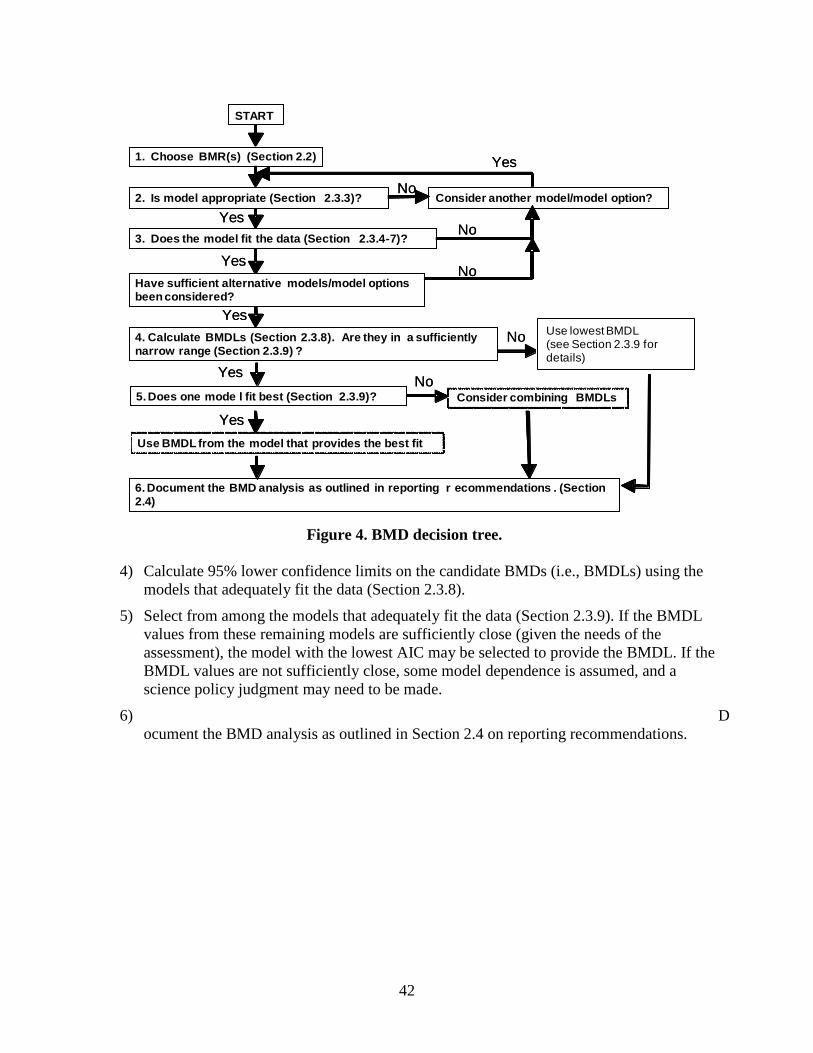
42

Figure 4. BMD decision tree.

4) Calculate 95% lower confidence limits on the candidate BMDs (i.e., BMDLs) using the models that adequately fit the data (Section 2.3.8).

5) Select from among the models that adequately fit the data (Section 2.3.9). If the BMDL values from these remaining models are sufficiently close (given the needs of the assessment), the model with the lowest AIC may be selected to provide the BMDL. If the BMDL values are not sufficiently close, some model dependence is assumed, and a science policy judgment may need to be made.

6) Document the BMD analysis as outlined in Section 2.4 on reporting recommendations.

3. Does the model fit the data (Section 2.3.4-7)?

4. Calculate BMDLs (Section 2.3.8). Are they in a sufficiently narrow range (Section 2.3.9) ?

Consider another model/model option?

5. Does one mode l fit best (Section 2.3.9)?

Yes

Yes

No

No

No

START

Use BMDL from the model that provides the best fit

YesConsider combining BMDLs

No

1. Choose BMR(s) (Section 2.2)

Yes

Yes

6. Document the BMD analysis as outlined in reporting r ecommendations . (Section 2.4)

Have sufficient alternative models/model options been considered?

No

Yes

2. Is model appropriate (Section 2.3.3)?

3. Does the model fit the data (Section 2.3.4-7)?

4. Calculate BMDLs (Section 2.3.8). Are they in a sufficiently narrow range (Section 2.3.9) ?

Consider another model/model option?

5. Does one mode l fit best (Section 2.3.9)?

Yes

Yes

No

No

No

START

Use BMDL from the model that provides the best fit

YesConsider combining BMDLs

No

1. Choose BMR(s) (Section 2.2)

Yes

Yes

6. Document the BMD analysis as outlined in reporting r ecommendations . (Section 2.4)

Have sufficient alternative models/model options been considered?

No

Yes

2. Is model appropriate (Section 2.3.3)?

Use lowest BMDL(see Section 2.3.9 for details)

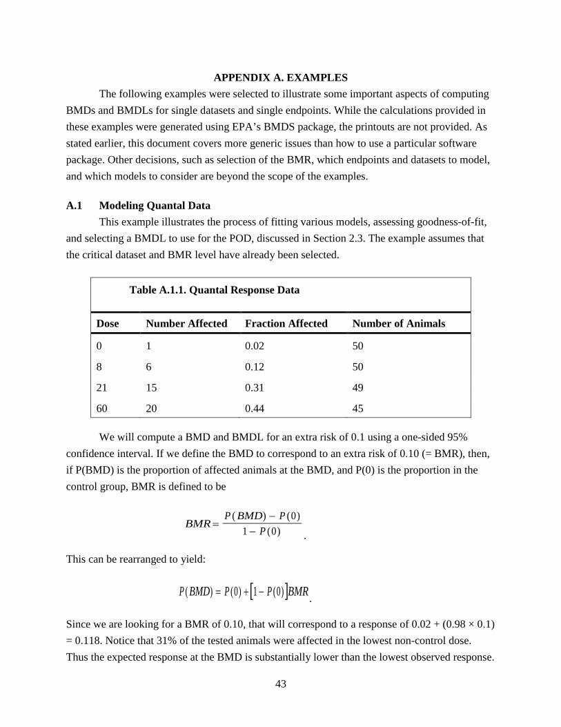
43

APPENDIX A. EXAMPLES The following examples were selected to illustrate some important aspects of computing BMDs and BMDLs for single datasets and single endpoints. While the calculations provided in these examples were generated using EPA’s BMDS package, the printouts are not provided. As stated earlier, this document covers more generic issues than how to use a particular software package. Other decisions, such as selection of the BMR, which endpoints and datasets to model, and which models to consider are beyond the scope of the examples. A.1 Modeling Quantal Data This example illustrates the process of fitting various models, assessing goodness-of-fit, and selecting a BMDL to use for the POD, discussed in Section 2.3. The example assumes that the critical dataset and BMR level have already been selected.

Table A.1.1. Quantal Response Data

Dose Number Affected Fraction Affected Number of Animals

0 1 0.02 50

8 6 0.12 50

21 15 0.31 49

60 20 0.44 45 We will compute a BMD and BMDL for an extra risk of 0.1 using a one-sided 95% confidence interval. If we define the BMD to correspond to an extra risk of 0.10 (= BMR), then, if P(BMD) is the proportion of affected animals at the BMD, and P(0) is the proportion in the control group, BMR is defined to be

BMRP BMD P

P=

−−

( ) ( )( )

01 0 .

This can be rearranged to yield:

Since we are looking for a BMR of 0.10, that will correspond to a response of 0.02 + (0.98 × 0.1) = 0.118. Notice that 31% of the tested animals were affected in the lowest non-control dose. Thus the expected response at the BMD is substantially lower than the lowest observed response.

[ ]P BMD P P BMR( ) ( ) ( )= + −0 1 0 .

44

Because of this, we need to be aware that model choice will have some effect on the BMD calculation. A.1.1. Selecting models to fit (Section 2.3.3) In this example, there is no reason (e.g., mechanistic) to apply one particular model, so we fit a number of models to the data, as shown in Table A.1.2. The different models will allow for a variety of curve shapes and low-dose behavior, which is reasonable given the uncertainty about which form of model can be expected to describe the data well. The models were fitted using constraints broadly considered to be consistent with biological processes (multistage model coefficients ≥0, power coefficient ≥1 for gamma and Weibull models, and slope coefficient ≥1 for the log-logistic model; see Section 2.3.3.3 and Appendix C). During estimation, the power coefficients were set to 1 (the constraint value) for the gamma and Weibull models, the log-logistic slope parameter was set to 1 (the constraint value) and the higher order multistage parameters β2 and β3 were set to 0 (the lower bound of the standard constraints). As a result, all fitted models required 2 degrees of freedom to estimate two parameters. We did not fit the quantal-linear or quantal-quadratic models, which are Weibull models with the exponent specified to be exactly 1 or 2, respectively. In this case, there was no basis for specifying the exponent parameter. Note that a desire for fewer parameters does not justify specifying the value of a parameter—there should be a good scientific basis for any specified parameters, and we usually lack such a basis. Also note that use of the 1st-order multistage model (which is also equivalent to the quantal-linear model) is the same as specifying the higher order multistage coefficients to be zero. A.1.2. Evaluating goodness-of-fit (Section 2.3.5) Table A.1.2 shows the results of fitting the models, which are sorted in order of increasing AIC. [Recall that AIC is -2 × (LL – p), where LL is the log-likelihood at the MLEs, and p is the number of parameters estimated; all else being equal, lower AIC values are preferred.] Five of the models have χ2values that exceed the recommended cutoff p-value of 0.1. Two models have p <0.10 and (not coincidentally) have at least one rather large scaled residual, indicating lack of fit to at least one data point (in this case, at the middle dose).

45

Table A.1.2. Goodness-of-Fit Statistics for the Models Fitted

Model χ2 p-value for χ2 AIC

Scaled residuals

dose 0 dose 8 dose 21 dose 60

log-logistica 0.96 0.618 173.6 -0.049 -0.151 0.772 -0.584

gammab 2.29 0.318 174.9 -0.304 0.182 1.186 -0.872

multistage (1st-order)c 2.29 0.318 174.9 -0.304 0.182 1.186 -0.872

Weibullb 2.29 0.318 174.9 -0.304 0.182 1.186 -0.872

log-probit 0.58 0.445 175.3 -0.035 -0.383 0.600 -0.273

probit 7.82 0.020 181.1 -1.688 0.012 2.125 -0.672

logistic 8.39 0.015 181.9 -1.801 -0.066 2.183 -0.613 a Slope parameter constrained to be ≥1. b Power parameters constrained to be ≥1. c The only multistage model to fit these data, given the standard constraints of non-negative

parameters. A.1.3. Comparing Models (Section 2.3.7) The model with the smallest AIC is the log-logistic model. For this model, the scaled residuals [i.e., (observed value − expected value)/SE are small (within ± 2 units; see Sections 2.3.5 and 2.5)] and a visual examination supports the choice of this model, since the predicted curve comes well within the confidence limits for each data point (Table A.1.2 and Figure A.1.1).

Next, notice that the next three models in Table A.1.2, the multistage, gamma, and Weibull, all give exactly the same fit and BMD prediction (as shown by the identical scaled residuals). In fact, for these data, they are really the same model: the multistage parameters were constrained to be positive, so β2 and β3 were set to zero, and the power parameters were set to the constraint value of 1, so all three models were estimated to be 0.0310 + [1 – 0.0310] × [1 − exp( – 0.110 Dose1)]. The AIC at 174.9 is only slightly worse than that for the log-logistic model, at 173.6. Figure A.1.2 shows the Weibull fit, representing all three fits. The fit at all doses is a little worse than it was for the log-logistic, apparent with close inspection of the graphs. Recall that it is the fit in the low-dose range that is usually of greatest interest in risk assessment applications (Section 2.3.5).

The log-probit model, shown in Figure A.1.3, also fits the data well, with small scaled residuals and with the predicted curve well within the confidence limits for each data point. It fits

46

slightly less well at the lowest dose than the models already discussed. Finally, the last two models in the table have p <0.10 and these can be ruled out of further consideration.

Figure A.1.1 Fit of log-logistic model. Error bars show 95% confidence limits on individual mean responses.

Figure A.1.2. Fit of Weibull model. Error bars show 95% confidence limits on individual mean responses.

0

0.1

0.2

0.3

0.4

0.5

0.6

0 10 20 30 40 50 60

Fra

ctio

n A

ffect

ed

dose

Log-Logistic Model with 0.95 Confidence Level

BMDL BMD

Log-Logistic

0

0.1

0.2

0.3

0.4

0.5

0.6

0 10 20 30 40 50 60

Fra

ctio

n A

ffect

ed

dose

Weibull Model with 0.95 Confidence Level

BMDL BMD

Weibull

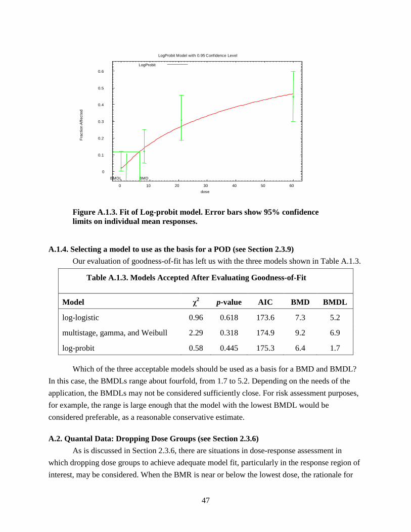
47

Figure A.1.3. Fit of Log-probit model. Error bars show 95% confidence limits on individual mean responses.

A.1.4. Selecting a model to use as the basis for a POD (see Section 2.3.9) Our evaluation of goodness-of-fit has left us with the three models shown in Table A.1.3.

Table A.1.3. Models Accepted After Evaluating Goodness-of-Fit

Model χ2 p-value AIC BMD BMDL

log-logistic 0.96 0.618 173.6 7.3 5.2

multistage, gamma, and Weibull 2.29 0.318 174.9 9.2 6.9

log-probit 0.58 0.445 175.3 6.4 1.7

Which of the three acceptable models should be used as a basis for a BMD and BMDL? In this case, the BMDLs range about fourfold, from 1.7 to 5.2. Depending on the needs of the application, the BMDLs may not be considered sufficiently close. For risk assessment purposes, for example, the range is large enough that the model with the lowest BMDL would be considered preferable, as a reasonable conservative estimate. A.2. Quantal Data: Dropping Dose Groups (see Section 2.3.6) As is discussed in Section 2.3.6, there are situations in dose-response assessment in which dropping dose groups to achieve adequate model fit, particularly in the response region of interest, may be considered. When the BMR is near or below the lowest dose, the rationale for

0

0.1

0.2

0.3

0.4

0.5

0.6

0 10 20 30 40 50 60

Fra

ctio

n A

ffect

ed

dose

LogProbit Model with 0.95 Confidence Level

BMDL BMD

LogProbit

48

eliminating data at the highest dose(s) is that the data at the highest dose may be the least informative of responses in the lower dose region of interest, i.e., near the BMR. This is true for both dichotomous and continuous data. The following example uses a dichotomous dataset to illustrate some basic principles to follow when considering whether to drop a dose group, including the evaluation of scaled residuals for comparison of low and high dose model fit. The subsequent example uses a larger dataset to demonstrate this and other considerations relevant to modeling mean and variance information for continuous data. The following dataset is an example of tumor response data that might be obtained from a chronic cancer bioassay that used a typical number of subjects per dose group for a chronic bioassay but more than the usual number of dose groups.

Table A.2.1. Quantal Response Data

Dose (ppm) Number affected Fraction affected Number of animals

0 0 0.00 50

50 1 0.02 50

100 10 0.20 50

150 35 0.7 50

250 30 0.75 40 As can be seen from an initial inspection of the data, response in terms of fraction affected seems to plateau at the highest doses. There could be a biological reason for this observation (e.g., a key enzyme that has become saturated), or the endpoint of interest could be masked at the highest dose by a more serious effect or by early mortality due to other causes (e.g. acute toxicity unrelated to tumor development), reducing the effective number at risk for the endpoint of interest. In the former case, one option would be to consider use of a model that contains an asymptote term, allowing for responses that may plateau prior to the 100% response level. However, if this type of model is not available, or if there is reason to be suspicious of the response reported at one of the doses (e.g., as a result of high mortality in the highest dose group) dropping a dose group may be an acceptable alternative approach. As in the previous example, we are assuming that the critical dataset and benchmark response level (BMR) have already been selected. Also for the purpose of this example, we are assuming an a priori selection of a model, the multistage model, after establishing the unavailability of a suitable biologically based model, or of time-of-death data for individual animals that would facilitate fitting a time-to-tumor model. First, we will attempt to fit all of the data. After evaluating the various multistage model options using the methods discussed in

49

Figure A.2.1. Fit of 3rd-order multistage model with highest dose group included. Error bars show 95% confidence limits.

Section 2.3.7 and illustrated in the previous example, the 3rd-order multistage model was chosen as the model that best fit the data in Table A.2.1. The plot for this model fit and goodness-of-fit p-value are shown in Figure A.2.1. Note that this model fit does not meet the goodness-of-fit criteria described in Section 2.3.5 (i.e., p-value is not greater than 0.05, the conventional p-value for an a priori selected model). The risk assessor has several choices in fitting an a priori selected model at this point, usually in the following order: (1) if there is a biological rationale for dropping a dose (e.g. high mortality in the highest dose group), drop it and refit the model of choice, (2) try another model, (3) choose another comparable dataset, or (4) drop a dose group and refit the model of choice. The highest dose group is ordinarily the one that is dropped when the BMR is near the low end of the data, as here (Section 2.3.6). However, other factors such as experimental error may provide justification for dropping a dose group other than the highest dose group. In this case, the highest dose group was dropped on the grounds that the high mortality was not relevant for fitting the dose-response at lower doses, and the multistage model was refit to the remaining four groups. The 3rd-order multistage model was determined to be the best fitting model to the data from Table A.2.1 without the highest dose (Figure A.2.2).

0

0.2

0.4

0.6

0.8

0 50 100 150 200 250

Frac

tion

Affe

cted

Dose

BMD BMDL

3° Multistage

p-value = 0.0057

50

Figure A.2.2. Fit of 3rd-order multistage model without the highest dose group. Error bars show 95% confidence limits.

Table A.2.2 shows the BMD, BMDL, p-value, and scaled residuals at all dose groups for the fit of the 3rd-order multistage model. Several aspects of this analysis support dropping the highest dose group data, including the inability to adequately fit the dose-response data for all five dose groups (p-value <0.05), acceptable fit (p-value >0.05) to the dose-response data when the highest dose group is removed, visual inspection of the plots (Figure A.2.1 versus Figure A.2.2), comparison of scaled residuals near the BMR (i.e., for the dose groups closest to the estimated BMD; −1.421 versus −0.650). In general, models that result in low scaled residuals for dose groups near the BMD are preferred. (See Sections 2.3.5 and 2.5.) Note that the model fit excluding the highest dose group is only suitable for characterizing the dose-response relationship for doses within the modeled range (Section 2.3.6).

0 0.1 0.2 0.3 0.4 0.5 0.6 0.7 0.8

0 20 40 60 80 100 120 140

Frac

tion

Affe

cted

Dose

BMD BMDL

3° Multistage

p-value = 0.5412

51

Table A.2.2. Comparison of 3rd-Order Multistage Models Fit With and Without High Dose

Fit statistics 3rd-Order with high dose 3rd-Order without high dose p-Value 0.0057 0.5412 BMD 59.4 70.1 BMDL 46.2 61.6 Scaled residual at 0 ppm 0.000 0.000 Scaled residual at 50 ppm −1.421 −0.650 Scaled residual at 100 ppm −0.939 −1.014 Scaled residual at 150 ppm 2.981 0.839 Scaled residual at 200 ppm −1.667 -- A.3. Continuous Data: Getting a Well-Fitting Model This example illustrates several considerations involved in fitting continuous models: the care required when using nonlinear (in parameters) modeling software, including variance modeling, and some of the data manipulation that may be required to get an adequate model fit for computing a BMD and BMDL, including dropping dose groups. In addition, two more technical points will be discussed here. First, convergence of a model that is nonlinear in parameters does not guarantee that MLEs have been achieved; sometimes some common sense and refitting is required to get MLEs. Second, once MLEs have been achieved, the model may not fit well enough and other actions may need to be taken to get a better fitting model.16

The data in Table A.3.1 represent a biochemical response in rats after dosing. For this example, we will compute a BMD as the dose where the mean response has been displaced by one control SD, as this document recommends for comparison purposes. As can be seen from Figure A.3.1, the dose-response data suggest a plateau. Thus, it may seem reasonable to fit a Hill model (available in BMDS). Other models could be considered, such as the exponential models in Appendix C, but for the purposes of this example the Hill model is used.

16 NOTE: Some of the behavior of this example depends on the way the April 3, 2000 version of the Hill model from BMDS selects its initial values. Other software, and even later versions of the Hill model from BMDS, may well behave differently using these data. This does not indicate “bugs” in the software, but rather, for some datasets, there can be multiple “local maxima” for the likelihood function; software that uses purely local methods for optimization (as does BMDS) can get trapped at a local maximum and may require experimenting with alternative initial parameter values to assure convergence to a true global maximum of the likelihood function. Software packages differ in the algorithm used to select the starting parameter values for optimization, so may end up in different local maxima.

52

Table A.3.1. Continuous Response Data

Dose Subjects/ group Mean SD

0. 8 100. 30.4

0.3 8 98.24 49.8

1. 8 111.34 59.9

3. 8 172.16 58.4

10. 8 357.48 167.5

30. 8 1695.03 260.9

100. 8 1576.11 169.7

300. 8 1896.22 141.7

Figure A.3.1. Mean and 95% confidence intervals for example data.

0

200

400

600

800

1000

1200

1400

1600

1800

2000

2200

-50 0 50 100 150 200 250 300 35

Mea

n R

espo

nse

dose16:31 09/11 2000

53

The variances in this dataset tend to increase as the means increase, which comports with the observation that it is common in biochemical data for the variance to be proportional to the square of the mean (approximately). For this example we fit a model to the data in which the variance is modeled as being proportional to the power of the mean. That is, our model is:

μ(d) = γ + V Xn / (k n + d n )

σ2(d) = α (μ(d))ρ, where d represents dose, μ(d) represents the mean response, and σ2(d) represents the variance of the observations at dose d. Among the remaining parameters, γ is the background response (or intercept), V the maximal response, k the dose where half the response has occurred, α a proportionality constant, and n and ρ exponents determined by the modeling process.

Rough estimates of this model’s parameters can be read off the graph of the data, providing a useful check of the fitting algorithm. When we fit a Hill model to the example data, we would expect γ (intercept) to be around 100 response units since that is about the background level of the response, V should be around 1,600 response since that is about the increment at the highest doses over the background level, and k should be in the range of 10–30 dose units. Furthermore, based on experience, n should be relatively small, say between 1 and 10, and ρ ought to fall between 1 and 2, or so, since as mentioned above, it is common for variances to be proportional to the square of means in such data. Using the April 3, 2000, version of the Hill model from BMDS, the fitting algorithm apparently converges on a solution. The parameter estimates from this solution are:

Table A.3.2. Parameter Estimates and Their Standard Errors for the Hill Model

Variable Estimate SE α 4381.57 2211.67 ρ 0.266572 0.0668979 intercept 105.045 22.8759 V 1634.05 51.087 n 4.76591 1.62145 k 14.256 1.80324 Log-likelihood = -345.786.

Note that all the estimates are in their expected ranges except for the estimate of ρ, which is 0.27, although we said we would have expected a value in the range 1–2.

The predicted values resulting from this model fit appear in Table A.3.3. While the model predicts the mean values and the SDs at the higher doses pretty well, the SDs at the lower doses

54

are overestimated by factors of 2 to 4. Since the BMR of 1SD is determined by the overestimated SD, the BMD1SD is predicted to be somewhat higher than the data suggest, and the BMDL1SD is likely to be mis-specified as well. While we could think about dropping the high dose(s) to improve the fit at lower doses, we will first continue with the full data set to illustrate another point.

Table A.3.3. Predicted Means and Standard Deviations, Based Upon the Hill Model, Compared to Observed Response Values

Dose N Observed

mean Observed

SD Estimated

mean Estimated

SD Scaled

Residual 0 8 100 30.4 105 123 −0.115

0.3 8 98.2 49.8 105 123 −0.156 1 8 111 59.9 105 123 0.138 3 8 172 58.4 106 123 1.518 10 8 357 168 360 145 −0.059 30 8 1700 261 1690 178 0.028 100 8 1580 170 1580 179 −2.570 300 8 1900 142 1740 179 2.483

This may be the best this model can do, but it looks suspiciously like the fitting algorithm was caught in a local maximum of the likelihood surface, and that, perhaps, if we could get better initial values for some of the parameters we could get a better set of estimates. Since the model for the mean seems to describe the data pretty well, we can refit the model by selecting the old estimates as initial values for the parameters of the model for the mean and obtaining new starting values for estimating the variance function parameters. These new estimates will come from regressing the log of the observed variance (that is, the square of the SD) on the log of the observed mean, i.e.,

where log denotes the natural logarithm. The parameter estimates from this regression are ρ=1.0,

log(α)=3.166, so the estimate of α is e3.166 = 23.7. Starting from these new values, the final estimates are shown in Table A.3.4, and the new predicted values appear in Table A.3.5. The BMD1SD is 7.3467 and the BMDL1SD is 5.96733 (not shown in the tables).

log( ) log( ) log( )var mean= +α ρ ,

55

Table A.3.4. New Parameter Estimates and Their Standard Errors for the Hill Model

Variable Estimate SE α 24.8892 24.5755 ρ 1.04671 0.162142 intercept 117.097 10.798 V 1629.2 64.9209 n 4.18855 1.33386 k 14.8385 1.86453

Table A.3.5. Predicted Means and Standard Deviations Based Upon the Final Hill Model, Compared to Observed Values

Dose N Observed

mean Observed

SD Estimated

mean Estimated

SD Scaled

Residual 0 8 100 30.4 117 60.3 −0.797

0.3 8 98.2 49.8 117 60.3 −0.882 1 8 111 59.9 117 60.3 −0.281 3 8 172 58.4 119 60.9 2.462 10 8 357 168 379 112 −0.556 30 8 1700 261 1670 242 0.351 100 8 1580 170 1750 248 −1.939 300 8 1900 142 1750 248 1.711

The log-likelihood for this fit is -333.2 (Table A.3.6), a substantial improvement over the previous fit. Furthermore, now not only do the estimated means agree better with those observed, but the estimated SDs are a lot closer to those observed. However, even though the fit is improved, neither the variance model (result of Test 3, below) nor the model for the mean (result of Test 4, below) fits the data, as the following excerpt from BMDS output for this example illustrates (Tables A.3.7, A.3.8):

Table A.3.6. Likelihoods of Interest

Model Log(likelihood) df (degrees of freedom) AIC

A1 −343.706 9 705.4 A2 −317.77 16 667.5 A3 −324.533 10 669.1 Fitted −333.127 6 678.3 R −458.043 2 920.1

56

Table A.3.7. Explanation of Tests

Test 1 Does response and/or variances differ among dose levels? (A2 vs. R) Test 2 Are variances homogeneous? (A1 vs. A2) Test 3 Are variances adequately modeled? (A2 vs. A3) Test 4 Does the model for the mean fit? (A3 vs. fitted)

Table A.3.8. Tests of Interest Test -2 × log(likelihood ratio) Test df p-value Test 1 280.547 14 <.0001 Test 2 51.8732 7 <.0001 Test 3 13.5263 6 0.0354 Test 4 17.1876 4 0.001777 What is going on? The table of fitted values above (Table A.3.5), particularly the column of scaled residuals, shows that the current model seriously under-predicts the response at a dose of 3 (scaled residual >2) and misses the response at the two highest doses on either side. Furthermore, the model over-predicts the SD at the two highest doses (which is probably why the model for the variance is rejected). The under-prediction at the lower doses is most important, however, because that is in the region of the BMD, as far as this fitted model can tell. What can be done? The three highest doses, at 30, 100, and 300, are quite far from the BMD; if we drop those doses, we will be eliminating doses with responses that the model cannot account for very well, and, since they are far from the BMD, we would not be eliminating much information about the actual location of the BMD. Furthermore, once the responses on the plateau have been dropped, other monotonic dose-response models can be fit to the data. In addition to the Hill model we consider a 1st-degree polynomial:

and the power model:

The linear polynomial model resulted after considering higher degree terms which did not add significantly to the model’s ability to fit the data. Note that, since this reduced dataset really contains no information about the maximum response V, the Hill model’s estimate of V is suspect (the estimate from the model reported in the

( )µ β β γd d= +0 1 .

( )µ β βd d= +0 1 ,

57

above table is excessively large: 143289; with a huge SE: 5.8 × 108). However, this does not affect the calculation at lower doses of a BMD corresponding to a BMR of one SD above the control mean for the reduced data set, because the BMR is distant from the region involving an asymptote.

All three models fit the reduced data well, according to both the summary results reported here (Table A.3.9) and a more detailed examination of the graphs and residuals (not shown here), but the AIC for the polynomial model is somewhat better than that for the other two, so that is the model we choose to calculate the BMD and BMDL. That is, the BMD and BMDL based on a one SD change are 1.46 and 1.11.

Table A.3 9. Final Model Comparison Model Goodness-of-fit p-value AIC BMD BMDL polynomial 0.98 375.5 1.46 1.11 power 0.95 377.4 1.66 1.11 Hill 0.76 379.4 1.70 1.14 This example illustrates three points, none of which is specific to modeling continuous data: (1) it is important to exercise some judgment when fitting models to data because no software package can guarantee that the parameters returned are actually MLEs, and the analyst may have to use trial and error to get an acceptable answer (e.g., by considering different initial values for model parameters); (2) we want models that describe the data well in the region of the BMR/BMD, which may involve some judicious narrowing of the dose range we attempt to model, if no other suitable models are available; and (3) it may be necessary to exercise some scientific judgment to compute BMDs for the BMR we want (e.g., identification of a suitable model to characterize variance heterogeneity and estimate the control SD adequately). What scientific and risk analytic judgment dictate as a desirable answer should not be subservient to what the software can do. A.4. Cancer Bioassay Data: Modeling to Obtain a POD for Linear Extrapolation This example uses a multistage model as typically constrained for dose-response modeling (i.e., model coefficients ≥0; see Example A.1). The multistage model has been U.S. EPA’s long-standing model for standard bioassay data,17

17 U.S. EPA used the linearized multistage model (which constrained model coefficients to be non-negative and the upper bound in the low-dose region to be linear), until the availability of the BMDS multistage model (which constrains only the model coefficients to be non-negative). A comparison of these two model forms using 102 data sets has shown them to provide virtually identical BMD10s and BMDL10s (Subramaniam et al. 2006).

in the absence of sufficient data to support a more biologically-based model. Under U.S. EPA’s 2005 cancer guidelines (U.S. EPA 2005a), quantitative risk estimates from cancer bioassay data are typically calculated by modeling the data in the observed range to estimate a BMDL for a BMR of 10% extra risk,

58

which is generally near the low end of the observable range for standard cancer bioassay data. This BMDL then serves as the POD for linear low-dose extrapolation to obtain a cancer potency estimate (i.e., unit risk or slope factor estimate). Note that with linear extrapolation, the choice of BMR ordinarily does not substantially affect the cancer potency estimate. However, when the mode of action of a carcinogen warrants a nonlinear approach, as discussed in U.S. EPA (2005a), the BMR value selected for the POD can have a significant impact on the final reference value. When a nonlinear approach is used, selection of the BMR includes consideration of the biological nature (e.g., severity) of the precursor effects being modeled and the statistical attributes of their dose-response relationships. (See Section 2.2.) This example uses the dose-response data presented in U.S. EPA’s Health and Environmental Effects Document for Dibromochloromethane (U.S. EPA 1988) for the quantitative estimate of carcinogenic risk from oral exposure. Summary information is available at U.S. EPA's IRIS Web site (http://www.epa.gov/iris/subst). The tumor endpoint was hepatocellular adenomas or carcinomas, in a cancer bioassay using B6C3F1 mice exposed by gavage. The rationale for study selection and endpoint selection, while an important component of any comprehensive write-up of a BMD calculation, is beyond the scope of this quantitative example.

Table A.4.1. Dose-Response Dataa Administered dose (mg/kg/day)

Human equivalent dose (mg/kg-day) Tumor incidence

0 0 6/50 50 2.83 10/49 100 5.67 19/50 a NTP (National Toxicology Program). (1988). Toxicology and carcinogenesis studies of chlorodibromomethane (CAS No. 124-48-1) in F344/N rats and B6C3F1 mice (gavage studies). TR-282. Available from http://ntp.niehs.nih.gov/ntp/htdocs/LT_rpts/tr282.pdf.

A BMR of 10% extra risk was selected, as it was near the low end of the observable range. While U.S. EPA’s cancer guidelines (U.S. EPA 2005a) emphasize that the choice of BMR should be independent of the extrapolation method, 10% extra risk is a typical BMR for standard cancer bioassay data when using linear extrapolation from the POD. The one-sided BMDL was calculated for the 95% confidence level. EPA’s cancer guidelines also recommend reporting an upper bound on the BMD, or a BMDU, in order to convey a measure of uncertainty. Accordingly, the 95% one-sided BMDU was also estimated. Together the two limits provide a 90% two-sided confidence interval. Model Fitting First, a 2nd-degree (i.e., n–1) multistage model was fitted to the data. The model form is

59

P(dose) = background + (1-background) × [1–exp(-beta1×dose1–beta2×dose2)].

This model fits all three observations exactly (Figure A.4.1, Table A.4.2); hence, the χ2

goodness-of-fit p-value is undefined and the scaled residuals are all zero. The AIC was 158.7. The BMD and lower and upper bounds (estimated by likelihood profile) estimates were:

BMD (ED10) = 2.91 mg/kg-day BMDL (LED10; 95% one-sided confidence limit) = 1.25 mg/kg-day BMDU (UED10; 95% one-sided confidence limit) = 4.59 mg/kg-day.

Figure A.4.1. Fitted 2nd-degree multistage model, and data means and standard errors.

60

Table A.4.2. Parameter Estimates With Standard Errors for 2nd-Degree Multistage Model

Parameter Maximum likelihood estimates (MLEs) SE

background 0.12 0.132665 beta1 0.00930036 0.141898 beta2 0.00925286 0.0246904 Next, a 1st-degree multistage model was fitted to the data to see if a more parsimonious model can also provide an adequate fit. The model form is:

P(dose) = background + (1–background) × [1–exp (-beta1×dose1)]. The 1st-degree multistage model also fit the data adequately (see Tables A.4.3 and A.4.4; Figure A.4.2), with a χ2goodness-of-fit p-value of 0.4494 and scaled residuals, shown in Table A.4.4, not unusually large. The AIC was 157.3. The BMD, BMDL, and BMDU estimates were:

BMD (ED10) = 1.88 mg/kg/day BMDL (LED10; 95% one-sided confidence limit) = 1.20 mg/kg-day BMDU (UED10; 95% one-sided confidence limit) = 4.59 mg/kg-day.

Table A.4.3. Parameter Estimates With Standard Errors for 1st-Degree Multistage Model

Parameter MLE SE background 0.111488 0.120556 beta1 0.0559807 0.0391492

Table A.4 4. Goodness-of-Fit Table

Dose Estimated probability

Expected number responding

Observed number responding Group size

Scaled residual

0.0000 0.1115 5.574 6 50 0.086 2.8300 0.2417 11.842 10 49 −0.205 5.6700 0.3531 17.657 19 50 0.118

61

Figure A.4.2. Fitted 1st-degree multistage model, and data means and standard errors.

Model Comparison The AIC is lower for the 1st-degree model suggesting that this is the preferred model. Because the multistage model is a family of k-degree models that can be compared statistically, a likelihood ratio test can also be used to evaluate whether the improvement in fit afforded by estimating additional parameters is justified. In this case, the log likelihood for the 2nd-degree model was -76.3439 and for the 1st-degree model was -76.6361. Thus twice the absolute difference in the log likelihoods is less than 3.84, a χ2 with one degree of freedom (i.e., 2–1), suggesting that the 1st-degree multistage model is not significantly different from the 2nd-degree model. Selecting a Model to Use for POD Computation Under the recommendations of this benchmark dose guidance, the more parsimonious 1st-degree model would be generally preferred. Final judgment on this may be subject to endpoint-specific guidance. In this example, then, the BMDL from the 1st-order model (1.20 mg/kg-day) would be used as the POD.

62

A.5. Developmental Toxicity Data In general, data from developmental toxicity studies in rodents are best modeled using nested models. These models account for any intra-litter correlation, or the tendency of littermates to respond more similarly to one another relative to the other litters in a dose group. If this correlation (which may vary with dose) is not estimated, variance estimates, and hence the confidence limits on benchmark responses and doses, will generally be mis-specified. In addition, these models often include provision for a litter-specific covariate, such as initial dam weight, which may be correlated with the outcome of interest (but not with the treatment) and may help clarify the response pattern. This example highlights the evaluation of these parameters in selecting suitable model fits. This example uses dose-response data reported by George et al. (1992), regarding the developmental toxicity of ethylene glycol diethyl ether administered orally to mice on days 6–15 of gestation. (See Table A.5.1.) As with other examples in this guidance, this example illustrates fitting a model to one dose-response pattern, here the nested logistic model. This model fits a wide variety of dose-response shapes for nested data. Note that the rationale for study selection and endpoint selection, while important components of any comprehensive BMD calculation write-up, are beyond the scope of this quantitative example. The outcome modeled was prevalence of skeletal malformations, a quantal endpoint. Litter size, which did not show an association with increasing exposure level except at the highest dose, was considered as a litter-specific covariate. A BMR of 10% extra risk is assumed just for the purpose of this example. The nested logistic model demonstrated a reasonably good visual fit to the mean responses of the dose groups (not shown), with a goodness-of-fit p-value of 0.45. Before accepting this model fit, the importance of litter size and intralitter correlations was assessed. Since the coefficients which gauge the influence of litter size in predicting the response rate were fairly close to zero (0.0013 and -0.1507, respectively), suggesting that litter size was not important in this case, the model was re-fitted without litter size. The resulting fit yielded a p-value of 0.184, adequate for supporting BMD evaluation. Its AIC, at 450.6, was also slightly lower than that of the first fit, at 452.5, reflecting fewer parameters in the model. Next, the intralitter correlations were assessed by setting the intralitter correlations (the coefficients phi1 – phi5) to zero. This fit was not successful, with a goodness-of-fit p-value of 0 and an AIC of 570.4 (compare to 450.6, above). The intralitter correlations are, therefore, important for describing the observed variability in this dataset. Consequently, the model incorporating intralitter correlations but not the litter-specific covariates was selected. The fitted model and the mean responses by dose group are shown in Figure A.5.1.

63

Table A.5.1. Dose-Response Data for Skeletal Malformations Resulting From Ethylene Glycol Diethyl Ether Administered Orally to Mice on Days 6–15 of Gestation, George et al. (1992)

Dose

Litter-Specific

Covariate Litter

Size Number Affected Dose

Litter-Specific

Covariate Litter

Size Number Affected Dose

Litter-Specific

Covariate Litter

Size Number Affected

0 0 0 0 0 0 0 0 0 0 0 0 0 0 0 0 0 0 0 0 0 0

6 8 8 9 9

10 10 11 11 11 11 12 11 11 11 11 14 14 14 15 15 15

6 8 8 9 9 10 10 11 11 11 11 12 11 11 11 11 14 14 14 15 15 15

0 0 0 0 0 0 0 0 0 0 0 0 0 0 0 0 0 0 4 0 0 0

150 150 150 150 150 150 150 150 150 150 150 150 150 150 150 150 150 150 150 150 150

3 10 10 11 11 11 12 12 12 12 12 12 13 13 13 13 13 14 14 15 18

3 10 10 11 11 11 12 12 12 12 12 12 13 13 13 13 13 14 14 15 18

0 0 1 0 4 5 0 0 0 0 0 1 0 0 0 0 1 0 0 1 0

1000 1000 1000 1000 1000 1000 1000 1000 1000 1000 1000 1000 1000 1000 1000 1000 1000 1000 1000 1000 1000

3 3 3 3 3 9 9 9 10 10 10 10 11 11 11 12 12 12 13 13 14

3 3 3 3 3 9 9 9 10 10 10 10 11 11 11 12 12 12 13 13 14

3 3 3 3 3 8 9 9 5 7 8 10 5 11 11 7 11 12 8 13 13

50 50 50 50 50 50 50 50 50 50 50 50 50 50 50 50 50 50 50

2 5 9 9 9

10 10 11 12 12 12 12 13 13 13 13 13 14 15

2 5 9 9 9 10 10 11 12 12 12 12 13 13 13 13 13 14 15

0 0 0 0 0 0 0 0 0 0 0 0 0 0 0 0 0 0 0

500 500 500 500 500 500 500 500 500 500 500 500 500 500 500 500 500 500 500 500 500 500

6 8 9

10 10 10 11 11 11 11 11 11 11 12 12 12 12 12 12 13 13 15

6 8 9

10 10 10 11 11 11 11 11 11 11 12 12 12 12 12 12 13 13 15

0 0 6 0 0 2 0 0 1 2 3 4 7 0 0 0 1 1 4 0 6 0

64

Figure A.5.1. Fraction of pups with skeletal malformations, and fitted nested logistic model.

A.6. Human Data Opportunities for modeling human toxicological data are limited, and the human studies are less standardized than studies of experimental animals; thus modeling of human data is done on a case-specific basis. Furthermore, modeling human data often involves adjusting for covariates. Additionally, for effects that are generally associated with older ages (e.g., most cancers and cardiovascular diseases), life table analyses are typically performed (See, for example, the cancer modeling in Section 10.1 of U.S. EPA’s 1,3-butadiene assessment (U.S. EPA 2002b)). For some other examples of benchmark dose modeling of human data, please refer to the following references. One example presented in U.S. EPA’s IRIS database is for peripheral nervous system dysfunction induced by carbon disulfide in occupationally exposed workers (U.S. EPA 1995b). Another example in IRIS is for developmental neurologic abnormalities in human infants from exposure to methylmercury (U.S. EPA 1995c). More recent examples of benchmark dose modeling of methylmercury-associated developmental neurologic effects from different human databases are reported by Budtz-Jorgensen et al. (2000) and van Wijngaarden et al. (2006). An example of benchmark dose modeling of developmental

0

0.2

0.4

0.6

0.8

1

0 200 400 600 800 1000

Frac

tion

Affe

cted

dose

Nested Logistic Model with 0.95 Confidence Level

BMDL BMD

Nested Logistic

65

neurologic effects from human exposure to polychlorinated biphenyls is provided by Jacobson et al. (2002). Another recent example of benchmark dose modeling of human data is the modeling of cadmium-induced renal effects by Suwazono et al. (2006). Note that sometimes human toxicological data are reported in ways that are similar to the reporting of toxicological data for laboratory animals (e.g., grouped data for a subchronic effect, without covariates, and with average exposures provided for the dose groups) and, in these cases, this guidance document would be applicable (see, for example, the modeling of human data on absolute lymphocyte count in Section 5.1.2 of U.S. EPA’s benzene assessment (U.S. EPA 2002d)).

66

APPENDIX B. GLOSSARY The following definitions are provided for clarification of this document. Any inconsistency with other U.S. EPA documents is unintentional. See also glossaries at http://www.epa.gov/iris and http://sis.nlm.nih.gov/enviro/enviropubs.html. Note that these links were verified as correct at the time of document finalization. Additional Risk: Additional risk is the difference in risk (or in the probability of a response) between subjects exposed and those not exposed to a hazard (herein, a particular dose or concentration of a chemical). In the context of a bioassay and its dose-response analysis, it is the increment by which the probability of adverse response exceeds background probability, calculated as P(d)–P(0), where P(d) is the probability of response risk at a dose d and P(0) is the probability of response at zero dose (i.e., background risk). Also see Extra Risk. Akaike Information Criteria (AIC): A measure of information loss from a dose-response model that can be used to compare a specified set of models. The AIC is defined as -2 × (LL - p), where LL is the log-likelihood of the model given the data, and p is the number of estimated parameters included in the model. Among a set of specified models, the model with the lowest AIC is the “best.” Asymptotic Test: Statistical tests for which the distribution of the test statistic converges to a known distribution as sample sizes increase without limit. Thus the limiting distribution can be used as an approximation for testing hypotheses. Bayesian: Involving statistical methods that assign probabilities or distributions to parameters (such as a population mean or model parameters) based on prior data collection and that apply Bayes’ theorem to revise the probabilities and distributions after obtaining additional experimental data. Benchmark Concentration (BMC): A concentration of a substance that when inhaled produces a predetermined change in the response rate of an adverse effect relative to the background response rate of this effect. This predetermined change is called a “benchmark response” or BMR. Benchmark Dose (BMD): A dose of a substance that when ingested produces a predetermined change in the response rate of an adverse effect relative to the background response rate of this effect. This predetermined change is called a “benchmark response” or BMR. Benchmark Response (BMR): A predetermined change in the response rate of an adverse effect relative to the background response rate of this effect. The BMR is the basis for deriving BMDs and BMDLs. Beta-Binomial Distribution: A statistical distribution sometimes used to represent clustered or nested values, e.g., measures on offspring in a litter, where the average proportions of an event for clusters are described by a Beta distribution and the numbers of events in a cluster are described by a binomial distribution.

67

Binomial Distribution: The statistical distribution of the probabilities of observing 0,1,2,…,n events from a sample of n independent trials each with the same probability that the event occurs. BMCL: A lower one-sided confidence limit on the benchmark concentration (BMC). BMDL: A lower one-sided confidence limit on the benchmark dose (BMD). BMDU: An upper one-sided confidence limit on the benchmark dose (BMD). Bootstrap: A statistical technique based on multiple resamplings, with replacement, of the observed values (nonparametric bootstrap). In the parametric bootstrap, a probability distribution estimated from the observed values is used to generate new samples. For example, based on a random sample of heights for 20 people (in some well-defined population), we might re-sample the data 5,000 times with replacement, calculating a standard deviation and a mean each time. The resulting distribution of some quantity of interest (e.g., the standard deviation or the mean) is used to calculate confidence limits or perform statistical tests in computationally complex situations, or where a particular distribution of an estimate or test statistic cannot be assumed. Cancer Potency (Cancer Slope Factor): A value that expresses the incremental increased risk of cancer incidence from a lifetime exposure to a substance per unit dose. Cancer potency is typically expressed in units that are the inverse of dose units. It can be multiplied by a given dose to quantify the lifetime cancer risk at that dose. In practice, it may be based upon an estimated upper bound rather than on an expected value. Categorical Data: Data recorded in categories, either without a natural ordering (nominal, e.g., tinker, tailor, or spy), or naturally ordered (ordinal, e.g., mild, moderate, or severe). Central Estimate: An estimate of the mean or median value of a set of data. Chi-square Goodness-of-Fit Test: A statistical hypothesis test used to compare observed counts with predicted numbers of independent observations classified into two or more categories. The total count is assumed to be fixed (and in multi-way classifications, sometimes the marginal counts are fixed). In the context of dose-response modeling, this test is often used to determine whether the observed response rates at each dose differ significantly from the corresponding predicted (or expected) response rates based on a selected model. Large deviations of observed from expected response rates yield large chi-square values, and indicate lack of fit of the selected model. For example, a model for the probability of an outcome in relation to dose might be used to predict the number of animals out of 50 that will respond at each of four dose levels (the categories), generating expected numbers (which may be fractional). The chi-square statistic is calculated as the sum (across the four doses) of the squared deviations of observed counts from expected numbers, each divided by the expected number. The exact distribution of the statistic, if the model is correct, is multinomial. For large samples (and with reasonably large response probabilities), the distribution approaches that of the chi-square distribution. For small samples, Fisher's exact test may be used as an alternative.

68

Clustered Data: Measurements collected on individuals that occur in groupings or clusters, e.g., littermates in reproductive and developmental studies. Circumstances common to members of the group (maternal environment, inherited traits, conditions of rearing) may exert a common influence upon outcomes of experimental treatments, leading to greater similarity in response between the members of a group. Statistical models of response that account for outcomes in such experiments will adjust for both the within-group and between-group variability of responses. Concave—see Convex Confidence Interval (Two-Sided): A statistically derived interval (consisting of lower and upper bounds) that has a specified probability of bounding the true value of some estimated parameter, if the same population is sampled repeatedly and an unbiased estimate of the parameter is calculated from each sample. Any particular confidence interval, based upon one sample, may or may not contain the true parameter value. The interval is expected to include the true value of the estimated parameter with a specified confidence, e.g., 95% of such intervals are expected to include the true value of the estimated parameter. Confidence Interval (One-Sided): A confidence interval that includes either the upper or the lower limit, but not both. For example, a one-sided upper confidence interval for the dose associated with a 10% increase in extra risk (BMD10) is reported by stating the upper limit (BMDU), 12.5 mg/kg-day. The other end of the interval is either the mathematical or natural (e.g., zero dose) lower limit. A one-sided lower confidence interval is reported by giving the lower limit (BMDL), e.g., 2.67 mg/kg-day, with it being understood that the interval extends to the mathematical (infinity) or natural upper limit. In reporting confidence limits for the BMD, it is important to report both the confidence level and the BMR. Confidence Limit: The lower and/or upper bound of a confidence interval (see Confidence Interval). Constrained Dose-Response Model: A model for which estimates of one or more parameters of the model are restricted to a specified range, e.g., equal to or greater than zero. Continuous Data: Data measured on a continuum, e.g., organ weight or enzyme concentration, as opposed to categorical data where data are recorded in categories (see Categorical Data). Convergence: In the case of a parameter estimate, approach to a single value with increasing sample size or increasing number of computational iterations. Convex: A function is convex (in some interval of its domain) if a line (chord) connecting any two function values, lies on or above the function values. Thus, for an increasing function of x, the slope increases as x increases. For example, the surface of a ski-jump or skateboard ramp is convex, while the top of an egg is concave. “Sublinear” is a synonym for convex peculiar to dose-response analysis, while “supralinear” is the corresponding synonym for concave. The notion behind these terms is that the dose-response curve may lie below or above a straight line drawn from the intercept (not necessarily zero) to some point on the curve that is of interest (e.g., the BMD or other POD).

69

Correlated Binomial Distribution: A statistical distribution typified by clustered data in which the individual members in a cluster, e.g., a litter, each have the same probability of showing an effect. Covariate: An independent variable other than dose that may influence the effect of interest, e.g., age, body weight, or polymorphism. Coverage Probability: The actual (as opposed to theoretical) probability that a population parameter is bounded by the limits of a given confidence interval procedure (see Confidence Interval). Cubic (Cubic Term in a Model): A model term (e.g., dose) raised to the third power (X3). May also refer to the highest-order term in a model (e.g., a + bX + cX2 + dX3 may be referred to as a cubic model, equation, or expression). Degrees of Freedom: For dose-response model fitting, “degrees of freedom” is the number of data points minus the number of model parameters estimated from the data. Delta Method: A method of approximating, by a truncated Taylor series, the central moments (e.g., the variance) of a function of a random variable in terms of the moments of that random variable. Dichotomize: The process of dividing or classifying objects, data, or events into two groups. For example, 50 animals could be classified into two groups, according to whether their weight exceeds some specified value. Dichotomous Data: A type of categorical data where an effect may be classified into only one of two possible outcomes, e.g., dead or alive, with or without tumor. Dispersion: A general term for the variation of a quantity around its central (mean or median) value. Dose-Response Model: A mathematical relationship (function) that quantitatively relates (predicts) a measure of an effect to a dose. Dose-Response Trend: A qualitative relationship between a biological response and dose in which the incidence or severity of the response increases or decreases with increasing dose. ECP: The concentration corresponding to a P% increase in an adverse effect, relative to the control response. Often used for inhalation exposures based on the airborne concentration. EDP: The dose corresponding to a P% increase in an adverse effect, relative to the control response. Often used for oral exposures based on administered dose. Estimate: Typically, a sample value intended to represent an unknown population parameter. Ordinarily, it will be based upon an Estimator (q.v) applied to sample data.

70

Estimator: A procedure, formula, or value used to derive an estimate of an unknown population parameter from sample data. For example, the sample mean is an estimator of the population mean. An essential part of mathematical statistics is finding estimators having desirable properties (e.g., accuracy and precision). Excess Risk: The increase in risk of experiencing an adverse effect relative to a comparison group, e.g., Additional or Extra Risk. Extra Risk: A measure of the proportional increase in risk of an adverse effect adjusted for the background incidence of the same effect. In other words, the ratio between the increased risk above background for a dose (d) divided by the proportion of the population not responding to the background risk. Extra risk is calculated as follows: [P(d)–P(0)] / [1–P(0)]. Also see Additional Risk. Frank Effect: An overt or clinically apparent toxic effect. Gamma Distribution: A unimodal statistical distribution (relative proportion of responders as a function of some measure, e.g., dose) that is restricted to effects greater than or equal to zero that can describe a wide variety of functional shapes, e.g., flat, peaked, or asymmetrical. Gaussian (Normal) Distribution: A unimodal, symmetrical, bell-shaped distribution centered around the mean (average) and having spread or dispersion measured by the standard deviation. Generalized Estimating Equation (GEE): A statistical technique used for estimating parameters in a model that requires only specification of the first two moments of the distribution, as compared to a complete specification of the distribution (as in maximum likelihood estimation). Goodness-of-Fit Statistic: A statistic that measures the deviation of observed data from predicted or hypothesized values. Some goodness-of-fit statistics can be used in statistical hypothesis tests, leading to rejection (or failure to reject) a model due to lack of an adequate fit. Hazard Identification: The identification of adverse effects that may result from exposure to a chemical hazard, including a qualitative description of the effects that may occur in humans. Hill Equation: A dose-response function, frequently used for enzyme kinetics, that monotonically approaches an asymptote (a maximum value) as a function of dose (d) raised to a power. The function is: F(d) = γ + ν dn / [ kn + dn] Hybrid Model: A model that establishes abnormal values for continuous data based on the extremes in controls (unexposed humans or animals) and which estimates the risk of abnormal response levels as a function of dose. Incidence: The number of new cases arising over a specific period of time, for a given number of subjects or a specified population. Describes the rate of onset or appearance of new cases among those susceptible (not already affected and still alive) during the time period. Also

71

expressed as a rate (e.g., per animal per 104 weeks; per 100,000 persons per year). Cumulative Incidence is the proportion of a specified population that will exhibit a condition (e.g., a cancer or disease) over a specified period of time (e.g., the number of test animals exhibiting liver cancers during a 2-year study in a given dose group). Independence: Two events are independent if the probability of either is the same whether or not the other occurs. In an experimental or observational study, this would mean that a result (outcome) in one animal or individual does not influence the probability of the same outcome occurring in another animal or individual. Intercept Term: In a dose-response model, the estimated value at zero dose or the dose corresponding to a zero effect. Least Squares: A statistical procedure that estimates the parameters of a model by minimizing the sum of squares of deviations of the observed data points from their estimated values based on the model, i.e., it minimizes the estimated residual variance. Likelihood: A number proportional to the probability (represented by the likelihood function) of observing a given set of data, assuming that a specified probability model and the hypothetical parameter values are correct. Note that this is conditional on the observed data, the model, and some particular values for model parameters. The method of maximum likelihood chooses those parameter values that maximize the value of the likelihood function. Likelihood Ratio Test: A statistical hypothesis test based on the ratio of the maximum likelihood of the data based upon a general model to that of the maximum likelihood for another, more restricted model. For example, one might test the hypothesis that the 2nd-order coefficient of a multistage model is zero, using the ratio of the maximum likelihoods for 1st-order and 2nd-order multistage models. The quantity -2 log(L1/L2) is distributed asymptotically as a χ2variate (with degrees of freedom equal to the difference in number of parameters estimated for L1 and L2). Linear Dose-Response Model: A mathematical relationship in which a change in response is proportional to a fixed amount of change in dose, e.g., Response = a + b × Dose. This is in distinction from a more general linear mathematical model, which is a linear combination of parameters. Lowest Observed Adverse Effect Level (LOAEL): The lowest exposure level at which there is biologically significant increases in frequency or severity of adverse effects between the exposed population and its appropriate control group. Local Maximum Solution: A mathematical solution for the maximum of a function in a local region of the parameter space, which may or may not be the overall (global) maximum across the allowable parameter space. Numerical algorithms that find solutions to BMD models (e.g., maximum likelihood estimates of parameters) may not always find the global maximum, especially for nonlinear models, which motivates the advice to test the obtained solution by restarting the maximization process using different initial values for the parameters.

72

Logistic Model: A particular form of a sigmoid (S-shaped) function that relates the proportion of individuals with a specified characteristic to an independent variable, e.g., dose (d). The function is: P(d) = 1/[1 + exp{-α – β × Dose}] Log Transformation: The process of taking logarithms of the data. The log transformation is sometimes applied to continuous response data (a) to make the transformed responses satisfy a normality assumption, if the raw data are lognormally distributed, or (b) to obtain a transformed response for which variances are more nearly the same in all the dose groups (assumption of homogeneous variances). Maximum Likelihood Estimate (MLE): Estimate of a population parameter (under a specified model for sampling error), found by maximizing the likelihood function, that is most likely to have produced the sample observations. Michaelis-Menten Equation: An equation frequently used to describe enzyme kinetics, having a maximum slope at zero dose, and approaching a maximum value asymptotically as dose increases. Margin of Exposure (MOE): Ratio of a dose that produces a specified effect, e.g., a benchmark dose, to an expected human dose. Alternatively, the LED10 or other point of departure divided by the actual or projected environmental exposure of interest. Monotonic Dose-Response: A dose-response curve that never decreases (or increases) as dose increases (or decreases). Multinomial Classification: A classification of animals or subjects into more than two categories, e.g., in a reproductive study fetuses may be classified as: dead, alive and normal, or alive and abnormal. No Observed Adverse Effect Level (NOAEL): The highest exposure level at which there are no biologically significant increases in the frequency or severity of adverse effects between the exposed population and its appropriate control; some effects may be produced at this dose level, but they are not considered adverse or precursors of adverse effects. Nonlinear Dose-Response Model: A mathematical relationship or model that cannot be expressed simply as the change in response being proportional to a fixed amount of change in dose. Examples of nonlinear dose-response models are (1) Response = a + b × Dose2, and (2) Response = a + b × log{Dose}. Note that this is in distinction from a more general nonlinear mathematical model, which is a nonlinear combination of parameters. Objective Function: A function that is to be maximized or minimized (e.g., the likelihood, in maximum likelihood estimation). Ordinal Data: Data that can be ordered or ranked. P-Value: In testing a hypothesis, the probability of a type I error (false positive), that is, the probability of rejecting the null hypothesis when the null hypothesis is true.

73

Parameter: A measurable or quantifiable characteristic of a system (e.g., a dose-response relationship, a probability distribution). In modeling, parameters usually are unknown and must be estimated based on samples of measurements, using Estimators. Percentile: The k-th sample percentile of a set of n measurements arranged in order of magnitude is that value that has k% of the measurements below it and (100-k)% above it. As a population parameter, the k-th percentile is the value x in the range of a probability distribution function that corresponds to a cumulative probability (k/100), with k = 1, 2, ... , 98, 99. Point of Departure (POD): The dose-response point that marks the starting point for low-dose extrapolation. The POD may be a NOAEL/LOAEL, but ideally is established from BMD modeling of the experimental data, and generally corresponds to a selected estimated low-level of response (e.g., 1 to 10% incidence for a quantal effect). Depending on the mode of action and other available data, some form of extrapolation below the POD may be employed for estimating low-dose risk or the POD may be divided by a series of uncertainty factors to arrive at a reference dose (RfD). Polynomial (in one variable): A mathematical function consisting of a sum of powers of a variable multiplied by coefficients, e.g., a + bx2 + cx3; also called a multinomial. The highest power is the order of a (univariate) polynomial. Probability: The chance of a particular outcome or event occurring. Probability takes on values between 0 and 1 with 0 indicating that the event never occurs and 1 indicating that the event always occurs. Probability Distribution: A statistical description (in the form of a distribution) of the relative probabilities of all possible outcomes of an event. Probit Function: A function derived assuming that the relative probabilities of effects as a function of dose are described by a Normal distribution. The cumulative probability as a function of dose has a sigmoid shape. The probit dose-response function is P(d) = Ф(α + β × dose ), where Ф is the cumulative standard normal or error function. Profile Likelihood: (1) The profile likelihood method employs the asymptotic distribution of the likelihood to test hypotheses about and construct confidence intervals for parameters or functions of parameters; (2) The likelihood profile is a plot of the values of the maximum of the likelihood function against fixed values of a parameter. Quadratic Term: A variable in a mathematical function that is raised to the second power. Quantal Data: Data representing an all-or-none effect, such as presence or absence of a particular type of tumor, or a normal versus abnormal level of a hormone; see Dichotomous Data.

74

Quantile: A specific percentile in the range of a probability distribution function. For example, the quantile of the χ2e distribution with 1 degree of freedom associated with the cumulative probability 0.95 (i.e., Pr{χ ≤ X} ≥ 0.95) is 3.84 (rounded). Quasi-Likelihood: A likelihood function that is not completely defined and generally based on only an expression including the mean and variance. Regression Analysis: A statistical procedure that estimates a mathematical function (regression equation) that quantitatively relates a dependent variable (biological effect) to an independent variable, e.g., dose, exposure duration, or age. Repeated Measures: A biological endpoint that is measured in the same subject at different times (e.g., body weight at different ages). Residual Variance: The variance (see Variance) in an experimental measurement remaining after accounting for variance due to the independent variables, e.g., dose, exposure duration, and age. Residuals: The numerical differences between observed and estimated values, usually in the context of regression analysis. See Scaled Residuals. Reference Concentration (RfC) or Reference Dose (RfD): An estimate of the concentration or dose of a substance (with uncertainty spanning perhaps an order of magnitude) to which a human population can be exposed (including sensitive subgroups) that is likely to be without an appreciable risk of deleterious effects during a lifetime. Risk: Probability that an animal or human exhibits a particular adverse effect under specified conditions of exposure; typically expressed on a scale of 0 to 1. Risk Characterization: The final step in the risk assessment process that involves the integration of information on hazard, exposure, and dose-response, to provide an estimate of the likelihood that any of the identified adverse effects will occur in humans. Scaled Residuals: In this document, scaled residuals are residuals that have been standardized by dividing by their standard errors (SE)—i.e., observed minus predicted response divided by SE. Second Degree: A mathematical function that contains a quadratic or squared term. Shape Parameter: The exponent of dose in a dose-response function that dictates the curvature of the function. Significance (Statistical Significance): See P-value. Sublinear, Supralinear, Convex, Concave: see entry for Convex. Threshold Dose: The dose below which a specified biological effect does not occur.

75

Uncertainty: Uncertainty can be defined as a lack of precise knowledge as to what the truth is, whether qualitative or quantitative (NRC, 1994). Uncertainty differs from Variability (q.v.) in that it can generally be reduced by further research. Uncertainty Factor: A numerical value (often a factor of 3 or 10) used to adjust a NOAEL, LOAEL, or benchmark dose in order to derive an RfC or RfD. Uncertainty factors are applied as needed to account for extrapolation of results in experimental animals to humans, interindividual variability including sensitive subgroups, extrapolation from a LOAEL to a NOAEL, extrapolation of results from subchronic exposures to chronic exposures, and database inadequacies. Unconstrained Model: A model with no restrictions imposed on the parameter space and thus, on the parameter estimates. Upper-Tail Probability: Probability that a variable exceeds a specified value. Variability: Inherent observable diversity (often among individuals) in biological sensitivity or response, as well as in exposure characteristics (such as breathing rates and food consumption). These differences can be better understood, but generally not reduced, by further research. Variance: A statistical measure of variability; the standard deviation squared. Weighted Least Squares Estimate: A parameter estimate obtained by minimizing the sum of squares of the observed minus the estimated values weighted by a function, typically the reciprocal of the variance of an observation.

76

APPENDIX C. SELECTED BENCHMARK DOSE MODELS Model descriptions for some of the models mentioned in this document are provided below. Additional information may be found, for example, in Filipsson et al. (2003). Quantal Models Here, 0 ≤ P(X) ≤ 1 is the probability of occurrence of a dichotomous outcome at dose X > 0. Parameter constraints given below assume increasing dose-response functions. Gamma Model P(X) = γ + (1–γ) [ Γ(α)-1 { 0∫βx tα-1 et dt} ], α ≥0, β > 0, 0 ≤ γ < 1

o γ is “background” o α is “power” – usually restricted to α ≥1 to avoid infinite slope approaching the origin o β is “slope”

Logistic Model P(X) = F{-(α + βX)}, 0 ≤ γ < 1, −∞ < α < +∞, β > 0 = F{-([X + (-α)(1/β)] / |1/β |) } where F{-(α + βX) } = [1 + exp{-(α + βX)}]-1 .

o α is “intercept” o β is “slope”

Log-Logistic Model P(X; γ, β) = γ + (1–γ) F{-(α + β lnX)}, 0 ≤ γ < 1, −∞ < α < +∞, β > 0 = γ + (1–γ) F{-([lnX – (-α)(1/β)] / (1/β))}, where F{-(α + β lnX)} = [1 + exp{-(α + βlnX)}]-1 .

o γ is “background” o α is “intercept” o β is “slope” – usually restricted to β ≥ 1 to avoid infinite slope approaching the origin

Multistage Model P(X) = γ + (1–γ) [1 – exp{- ∑ βj Xj }], j = 1, ..., k, 0 ≤ γ < 1

o γ is “background” o β1, …, βk are “slopes” – usually restricted to βj ≥ 0 to ensure monotonic curves

Probit Model P(X) = P(X; γ, β) = Φ{α + βX}, 0 ≤ γ < 1, −∞ < α < +∞, β > 0 = Φ{[X + (-α)(1/β)] / (1/β)}

o α is “intercept” o β is “slope”

77

Log-Probit Model P(X) = γ + (1–γ) Φ{α + β lnX}, 0 ≤ γ < 1, −∞ < α < +∞, β > 0 = γ + (1–γ) Φ{ [lnX – (-α)(1/β)] / (1/β)}

o γ is “background” o α is “intercept” o β is “slope”

Weibull Model P(X) = γ + (1–γ) [1 – exp{-βxα}], α ≥ 0, 0 ≤ γ < 1, β > 0

o γ is “background” o β is “slope” o α is “power” – usually restricted to α ≥ 1 to avoid infinite slope approaching the origin

Dichotomous Hill Model P(X) = v [1 + g exp{-(a + b log(X)}] / [1 + exp[-{a + b log(X)}]

o 0 ≤ g < 1, 0 < v ≤ 1, b ≥ 0 o v is the maximum probability of response predicted by the model o g multiplied by v (v × g) is the background estimate of the probability of response o b is “slope”

Nested Log-Logistic Model P(X) = α + θ1rij + [1 – α – θ1rij ] / [1 + exp{β + θ2 rij – γ log(X)}], if dose > 0 = α + θ1rij, if dose = 0

o rij is the litter-specific covariate for the jth litter in the ith dose group o α ≥ 0, β > 0, γ ≥ 0, and α + θ1rij ≥ 0 for every rij o α is “background” o β is “slope” o γ is “power”—usually restricted to γ ≥ 1 to avoid infinite slope approaching the origin

78

Continuous Models Here, μ(X) is the mean response at dose X > 0. The variance across dose groups can be modeled (e.g., as a power function of the mean) or assumed to be constant. Select approaches to modeling the mean responses are displayed below. Polynomial Continuous Model μ(X) = γ + ∑ βj X j, j = 1, ..., n

o βj are usually restricted to βj ≥ 0 (in the case of increasing response) or βj ≤ 0 (in the case of decreasing response data) to ensure monotonic curves

Power Continuous Model μ(X) = γ + β Xα, α > 0, β > 0

o γ is “background” o β is “slope” o α is “power”—usually restricted to α ≥ 1 to avoid infinite slope approaching the origin

Hill Continuous Model μ(X) = γ + ν Xn / (kn + Xn )

o γ is “background” o k is “slope” o ν is asymptote o n is “power”—usually restricted to n ≥ 1 to avoid infinite slope approaching the origin

Exponential Continuous Models, a set of nested models: Model 2: μ(X) = γ exp{sign k X} Model 3: μ(X) = γ exp{sign (k X)d} Model 4: μ(X) = γ (c – (c–1) exp{-1 k X}) Model 5: μ(X) = γ (c – (c–1) exp{-1 (k X)d})

o γ is “background” o b is “slope” o “sign” indicates the direction of change: +1 for increasing response, −1 for decreasing

response o c is an asymptote parameter (Models 3 and 5 only), with 0 < c < 1 for decreasing data o d is “power”—usually restricted to d > 1 (Models 3 and 5 only)

79

APPENDIX D. BENCHMARK DOSE TECHNICAL GUIDANCE DOCUMENT CONTRIBUTORS AND REVIEWERS

CONTRIBUTORS John Fox, Office of Research and Development, U.S. EPA, Washington, DC Allan Marcus, Office of Research and Development, U.S. EPA, Research Triangle Park, NC David Svendsgaard, Office of Research and Development, U.S. EPA, Research Triangle Park, NC Paul White, Office of Research and Development, U.S. EPA, Washington, DC

Diane Henshel, Office of the Science Advisor, U.S. EPA, Washington, DC EXTERNAL PEER REVIEWERS George Alexeef, Office of Environmental Health Hazard Assessment, California Environmental Protection Agency, Oakland, CA 94612 Kevin Brand, Department of Epidemiology and Statistical Medicine, University of Ottawa, Ottawa ON, K1N 5C8 Canada Paul Catalano, Department of Biostatistical Science, Harvard School of Public Health, Boston, MA 02115 Harvey Clewell, ICF Consulting, Ruston, LA George Daston, Miami Valley Laboratories, Proctor and Gamble, Cincinnati, OH Elaine Faustman, Department of Environmental Health, University of Washington, Seattle, WA Clay Frederick, Toxicology Department, Rohm and Haas Company, Spring House, PA Lynne Haber, Toxicology Excellence for Risk Assessment, Cincinnati, OH Dale Hattis (Workshop Chair), Center for Technology, Environment and Development, Clark University, Worcester, MA Colin Park, Consultant, Midland, MI Lorenz Rhomberg, Gradient Corporation, Cambridge, MA Robert Sielken, Jr., JSC Sielken, Bryan, TX William Slikker, Jr., U.S. Food and Drug Administration, Rockville, MD R. Webster West, Department of Statistics, University of South Carolina, Columbia, SC

80

Yiliang Zhu, Department of Epidemiology & Biostatistics, University of South Florida, Tampa, FL

81

REFERENCES Note: Weblinks provided below were accurate at the time of document finalization. Akaike, H. (1973) Information theory and an extension of the maximum likelihood principle. In: Petrov, BN; Csaki, F; eds. Proceedings of the second international symposium on information theory. Budapest, Hungary: Akademiai Kiado, pp. 267-281. Alexeeff, GV; Lewis, DC; Ragle, NL. (1993) Estimation of potential health effects from acute exposure to hydrogen fluoride using a ‘benchmark dose’ approach. Risk Anal 13(1):63-69. Allen, BC; Kavlock, RJ; Kimmel, CA; Faustman, EM. (1994a) Dose-response assessment for developmental toxicity: II. Comparison of generic benchmark dose estimates with NOAELs. Fundam Appl Toxicol 23:487-495. Allen, BC; Kavlock, RJ; Kimmel, CA; Faustman, EM. (1994b) Dose-response assessment for development toxicity: III. Statistical models. Fundam Appl Toxicol 23:496-509. Allen, BC; Strong, PL; Price, CJ; Hubbard, SA; Daston, GP. (1996) Benchmark dose analysis of developmental toxicity in rats exposed to boric acid. Fundam Appl Toxicol 32:194-204. Auton, TR. (1994) Calculation of benchmark doses from teratology data. Regul Toxicol Pharmacol 19:152-167. Bailer, AJ; Noble, RB; Wheeler, MW. (2005) Model uncertainty and risk estimation for experimental studies of quantal responses. Risk Anal 25:291-299. Bailer, AJ; Portier, CJ. (1988) Effects of treatment-induced mortality and tumor-induces mortality on tests for carcinogenicity in small samples. Biometrics 44::417-431. Barnes, DG; Daston, GP; Evans, JS; Jarabek, AM; Kavlock, RJ; Kimmel, CA; Park, C; Spitzer, HL. (1995) Benchmark dose workshop: criteria for use of a benchmark dose to estimate a reference dose. Regul Toxicol Pharmacol 21:296-306. Bates, DM; Watts, DG. (1988) Nonlinear regression analysis and its applications. New York, NY: Wiley. Beck, BD; Conolly, RB; Dourson, ML; Guth, D; Hattis, D; Kimmel, C; Lewis, SC. (1993) Symposium overview: improvements in quantitative noncancer risk assessment. Fundam Appl Toxicol 20:1-14. Benford, D; Bolger, PM; Carthew, P; Coulet, M; DiNovi, M; Leblanc, J-C; Renwick, AG; Setzer, W; Schlatter, J; Smith, B; Slob, W; Williams, G; Wildemann, T. (2010) Application of the Margin of Exposure (MOE) approach to substances in food that are genotoxic and carcinogenic. Food Chem Toxicol 48:S2-S24. Budtz-Jorgensen, E; Grandjean, P; Keiding, N; White,RF; Weihe, P. (2000) Benchmark dose calculations of methylmercury-associated neurobehavioural deficits. Toxicol Lett 112-113:193-199. California EPA (California Office of Environmental Health Hazard Assessment). (1994) Safety assessment for non-cancer endpoints: the benchmark dose and other possible approaches. Summary report. Catalano, PJ; Ryan, LM. (1992) Bivariate latent variable models for clustered discrete and continuous outcomes. J Am Stat Assoc 87:651-658. Catalano, PJ; Scharfstein, DO; Ryan, LM; Kimmel, CA; Kimmel, GL. (1993) Statistical model for fetal death fetal weight and malformation in developmental toxicity studies. Teratology 47:281-290. Chen, C; Farland, W. (1991) Incorporating cell proliferation in quantitative cancer risk assessment: approaches, issues, and uncertainties. In: Butterworth, B; Slaga, T; Farland, W; et al., eds. Chemical induced cell proliferation: implications for risk assessment. New York, NY: Wiley-Liss, pp. 481–499.

82

Chen, JJ; Kodell, RL. (1989). Quantitative risk assessment for teratologic effects. J Am Stat Assoc 84:966-971. Chen, JJ; Kodell, RL; Howe, RB; Gaylor, DW. (1991) Analysis of trinomial responses from reproductive and developmental toxicity experiments. Biometrics 47:1049-1058. Clayton, D; Hills, M. (1993) Statistical models in epidemiology. Oxford, UK: Oxford University Press. Crump, KS. (1984) A new method for determining allowable daily intakes. Fundam Appl Toxicol 4:854-871. Crump, KS. (1995) Calculation of benchmark doses from continuous data. Risk Anal 15:79-89. Crump, KS. (2002). Critical Issues in benchmark dose calculations from continuous data. Crit Rev Toxicol 32:133-153. Crump, KS; Hoel, DG; Langley, CH; Peto, R. (1976) Fundamental carcinogenic processes and their implications for low dose risk assessment. Cancer Res 36:2973-2979. Crump, KS; Howe, R. (1985). A review of methods for calculating statistical confidence limits in low-dose extrapolation. In: Clayson, DB; Krewski, D; Munro, I; eds. Toxicological Risk Assessment. Boca Raton, FL: CRC Press, Inc. Davidian, M; Giltinan, DM. (1995) Nonlinear models for repeated measurement data. London, UK: Chapman and Hall. Dourson, ML; Hertzberg, RC; Hartung, R; Blackburn, K. (1985) Novel methods for the estimation of acceptable daily intake. Toxicol Ind Health 1:23-41. Draper, N; Smith, H. (1981) Applied regression analysis. 2nd ed., chap 10. New York, NY: Wiley. Farmer, JH; Kodell, RL; Gaylor, DW. (1982) Estimation and extrapolation of tumor probabilities from a mouse bioassay with survival/sacrifice components. Risk Anal 2(1):27-34. Faustman, EM; Allen, BC; Kavlock, RJ; Kimmel, CA. (1994) Dose-response assessment for developmental toxicity: I. Characterization of data base and determination of NOAELs. Fundam Appl Toxicol 23:478-486. Filipsson, AF; Sand, S; Nilsson, J; Victorin, K. (2003) The benchmark dose method—a review of available models, and recommendations for application in health risk assessment. Crit Rev Toxicol 33:505-542. Filipsson, AF; Victorin, K. (2003) Comparison of available benchmark dose softwares and models using trichloroethylene as a model substance. Regul Toxicol Pharmacol 37:343-355. Fowles, JR; Alexeeff, GV; Dodge, D. (1999) The use of benchmark dose methodology with acute inhalation lethality data. Regul Toxicol Pharmacol 29:262-278. Fung, KY; Marro, L; Krewski, D. (1998) A comparison of methods for estimating the benchmark dose based on overdispersed data from developmental toxicity studies. Risk Anal 18:329-342. Gallant, AR. (1987) Nonlinear statistical models. New York, NY: Wiley. Gart, JJ; Krewski, D; Lee, PN; Tarone, RE; Wahrendorf, J. (1986) Statistical methods in cancer research. Vol. 3. The Design and Analysis of Long-Term Animal Experiments. Lyon, France: International Agency for Research on Cancer. Gaylor, DW. (1983) The use of safety factors for controlling risk. J Toxicol Environ Health 11:329-336. Gaylor, DW. (1992) Incidence of developmental defects at the no observed adverse effect level (NOAEL). Regul Toxicol Pharmacol 15:151-160.

83

Gaylor, DW. (1996) Quantalization of continuous data for benchmark dose estimation. Regul Toxicol Pharmacol 24:246-250. Gaylor, DW; Aylward, LL. (2004) An evaluation of benchmark dose methodology for non-cancer continuous-data health effects in animals due to exposures to dioxin (TCDD). Regul Toxicol Pharmacol 40:9-17. Gaylor, DW; Kodell, RL. (1980) Linear interpolation algorithm for low dose risk assessment of toxic substances. J Environ Pathol Toxicol 4:305–312. Gaylor, DW; Ryan, L; Krewski, D; Zhu, Y. (1998) Procedures for calculating benchmark doses for health risk assessment. Regul Toxicol Pharmacol 28:150-164. Gaylor, D; Slikker, W, Jr. (1990) Risk assessment for neurotoxic effects. Neurotoxicology 11:211-218. Gaylor, D; Slikker, W, Jr. (2004) Role of the standard deviation in the estimation of benchmark doses with continuous data. Risk Anal 24:1683-1687. Gehlhaus, MW; Gift, JS; Hogan, KA; Kopylev, L; Schlosser, PM; Kadry, AR. (2011) Approaches to cancer assessment in EPA’s Integrated Risk Information System. Toxicol Appl Pharmacol 254:170-180. George, JD; Price, CJ; Marr, MC; Kimmel, CA; Schwetz, BA; Morrissey, RE. (1992) The developmental toxicity of ethylene glycol diethyl ether in mice and rabbits. Fundam Appl Toxicol 19:15-25. Guth, DJ; Carroll, RJ; Simpson, DG; Zhou, H. (1997) Categorical regression analysis of acute exposure to tetrachloroethylene. Risk Anal 17:321-332. Hasselblad, V; Jarabek, AM. (1995) Dose-response analysis of toxic chemicals. In: Berry, DA; Stangl, DK; eds. Bayesian biostatistics. New York, NY: Marcel Dekker, Inc. Hertzberg, RC. (1989) Fitting a model to categorical response data with application to species extrapolation of toxicity. Health Physics 57:405-409. Hertzberg, RC; Miller, M. (1985) A statistical model for species extrapolation using categorical response data. Toxicol Ind Health 1:43-57. Jacobson, JL; Janisse, J; Banerjee, M; Jester, J; Jacobson, SW; Ager, JW. (2002) A benchmark dose analysis of prenatal exposure to polychlorinated biphenyls. Environ Health Perspect 110:393-398. Kang, SH; Kodell, RL; Chen, JJ. (2000) Incorporating model uncertainties along with data uncertainties in microbial risk assessment. Regul Toxicol Pharmacol 32:68–72. Kavlock, RJ; Allen, BC; Kimmel, CA; Faustman, EM. (1995) Dose-response assessment for developmental toxicity: IV. Benchmark doses for fetal weight changes. Fundam Appl Toxicol 26:211-222. Kavlock, RJ; Schmid, JE; Setzer, RW, Jr. (1996) A simulation study of the influence of study design on the estimation of benchmark doses for developmental toxicity. Risk Anal 16:391-403. Kimmel, CA; Gaylor, DW. (1988) Issues in qualitative and quantitative risk analysis for developmental toxicity. Risk Anal 8:15-20. Kimmel, CA; Wellington, DG; Farland, W; Rose, P; Manson, JM; Chernoff, N; Young, JF; Selevan, SG; Kaplan, N; Chen, C; Chitlik, LD; Siegel-Scott, CL; Valaoras, G; Wells, S. (1989) Overview of a workshop on quantitative models for developmental toxicity risk assessment. Environ Health Perspect 79:209-215. Kodell, RL; Chen, JJ; Gaylor, DW. (1995) Neurotoxicity modeling for risk assessment. Regul Toxicol Pharmacol 22:24-29.

84

Krewski, D; Brown,C; Murdoch, D. (1984) Determining "safe" levels of exposure: safety factors or mathematical models? Fundam Appl Toxicol 4:S383-S394. Krewski, D; Zhu, Y. (1994). Applications of multinomial dose-response models in developmental toxicity risk assessment. Risk Anal 14:613-627. Krewski, D; Zhu, Y. (1995) A simple data transformation for estimating benchmark doses in developmental toxicity experiments. Risk Anal 15:29-39. Kupper, LL; Portier, C; Hogan, MD; Yamamoto, E. (1986) The impact of litter effects on dose-response modeling in teratology. Biometrics 42:85-98. Lefkopoulou, M; Moore, D; Ryan, L. (1989) The analysis of multiple binary outcomes: application to rodent teratology experiments. J Am Stat Assoc 84:810-815. Leisenring, W; Ryan, L. (1992) Statistical properties at the NOAEL. Regul Toxicol Pharmacol 15:161-171. Liang, KY; Zeger, SL. (1986) Longitudinal data analysis using generalized linear models. Biometrika 73:13-22. Linhart, H; Zucchini, W. (1986) Model Selection. New York, NY: Wiley. McCullagh, P; Nelder, JA. (1989) Generalized linear models. 2nd ed. London, UK: Chapman and Hall. Mantel, N; Bryan, WR. (1961) Safety testing of carcinogenic agents. J Natl Cancer Inst 27:455-470. Moolgavkar, SH; Knudson, AG. (1981) Mutation and cancer: a model for human carcinogenesis. J Natl Cancer Inst 66:1037–1052. Murrell, JA; Portier, CJ; Morris, RW. (1998) Characterizing dose-response: I: Critical assessment of the benchmark dose concept. Risk Anal 18:13-26. NRC (National Research Council). (1983) Risk assessment in the federal government: managing the process. Washington, DC: National Academy Press. NRC. (1994) Science and judgment in risk assessment. Washington, DC: National Academy Press. Nitcheva, DK; Piegorsch, WW; West, RW; Kodell, RL. (2005) Multiplicity-adjusted inferences in risk assessment: benchmark analysis with quantal response data. Biometrics 61(1):277-286. Parham, F; Portier, C. (2005) Chapter 14: Benchmark dose approach. In: Edler, L; Kitsos, CP; eds. Recent advances in quantitative methods in cancer and human health risk assessment. Chichester, UK: John Wiley & Sons, Ltd; pp. 239-254. Piegorsch, WW; West, RW. (2005) Benchmark analysis: shopping with proper confidence. Risk Anal 25(4):913-920. Rao, JNK; Scott, AJ. (1992) A simple method for the analysis of clustered binary data. Biometrics 48:577-585. Ross, GJS. (1990) Nonlinear estimation. New York, NY: Springer-Verlag. Ryan, LM. (1992a) The use of generalized estimating equations for risk assessment in developmental toxicity. Risk Anal 12:439-447. Ryan, L. (1992b) Quantitative risk assessment for developmental toxicity. Biometrics 48:163-174.

85

Ryan, LM; Catalano, PJ; Kimmel, C; Kimmel, G. (1991) Relationship between fetal weight and malformation in developmental toxicity studies. Teratology 44:215-223. Sand, S. (2005) Dose-response modeling: Evaluation, application, and development of procedures for benchmark dose analysis in health risk assessment of chemical substances [Thesis]. Karolinska Institute, Stockholm, Sweden. Available online at: http://publications.ki.se/jspui/bitstream/10616/39163/1/thesis.pdf. Sand, S; Filipsson, AF; Victorin, K. (2002) Evaluation of the benchmark dose method for dichotomous data: model dependence and model selection. Regul Toxicol Pharmacol 36:184-197. Sand S; Victorin, K; Filipsson AF. (2008) The Current State of Knowledge on the Use of the Benchmark Dose Concept in Risk Assessment. J Appl Toxicol 28:405-421. Seber, GAF; Wild, CJ. (1989) Nonlinear regression. New York, NY: Wiley. Simpson, DG; Carroll, RJ; Zhou, H; Guth, DJ. (1996a) Interval censoring and marginal analysis in ordinal regression. J Agr Biol Environ Stat 1:354-376. Simpson, DG; Carroll, RJ; Zhou, H; Guth, DJ. (1996b) Weighted logistic regression and robust analysis of diverse toxicology data. Commun Statist Meth 25:2615-2632. Stone, M. (1998) Akaike's criteria. In: Armitage, P; Colton, T; eds. Encyclopedia of Biostatistics. New York, NY: Wiley. Subramaniam, RP; White, P; Cogliano, VJ. (2006) Comparison of cancer slope factors using different statistical approaches. Risk Anal 25(3):825-830. Suwazono Y; Sand S; Vahter M; Filipsson AF; Skerfving S; Lidfeldt, J; Akesson, A . (2006) Benchmark dose for cadmium-induced renal effects in humans. Environ Health Perspect 114:1072-1076. U.S. EPA (Environmental Protection Agency). (1986) Guidelines for carcinogen risk assessment. Federal Register 51(185):33992–34003. Available online at http://www.epa.gov/raf/pubalpha.htm. U.S. EPA. (1988) Health and environmental effects document for dibromochloromethane. Environmental Criteria and Assessment Office, Office of Health and Environmental Assessment, Cincinnati, OH; ECAO-CIN-GO40. Available from the National Technical Information Service, Springfield, VA. U.S. EPA. (1991) Guidelines for developmental toxicity risk assessment. Federal Register 56(234):63798-63826. Available online at http://www.epa.gov/raf/pubalpha.htm. U.S. EPA. (1994) Methods for derivation of inhalation reference concentrations and application of inhalation dosimetry. Environmental Criteria and Assessment Office, Office of Health and Environmental Assessment, Cincinnati, OH; EPA/600/8-90/066F. Available online at http://www.epa.gov/iris/backgrd.html. U.S. EPA. (1995a) Use of the benchmark dose approach in health risk assessment. Risk Assessment Forum, Washington, DC; EPA/630/R–94/007. Available online at. http://www.epa.gov/raf/pubalpha.htm. U.S. EPA. (1995b). Integrated risk information system (IRIS): Online substance file for carbon disulfide. Available at http://cfpub.epa.gov/ncea/iris/index.cfm?fuseaction=iris.showSubstanceList. U.S. EPA. (1995c). Integrated risk information system (IRIS): Online substance file for methylmercury). Available online at http://cfpub.epa.gov/ncea/iris/index.cfm?fuseaction=iris.showSubstanceList. U.S. EPA. (1996a) Guidelines for reproductive toxicity risk assessment. Federal Register 61(212):56274-56322. Available online at http://www.epa.gov/raf/pubalpha.htm.

86

U.S. EPA. (1996b) Report on the benchmark dose peer consultation workshop. Risk Assessment Forum, Washington, DC; EPA/630/R-96/011. Available online at http://www.epa.gov/raf/pubworkshop-rpts.htm. U.S. EPA. (1998) Guidelines for neurotoxicity risk assessment. Federal Register 63(93):26926-26954. Available online at http://www.epa.gov/raf/pubalpha.htm. U.S. EPA. (2002a) A review of the reference dose and reference concentration processes. Risk Assessment Forum, Washington, DC; EPA/630/P-02/002F. Available online at http://www.epa.gov/raf/pubalpha.htm. U.S. EPA. (2002b) Health assessment of 1,3-butadiene. National Center for Environmental Assessment, Washington, DC; EPA/600/P-98/001F. Available online at http://cfpub.epa.gov/ncea/iris/index.cfm?fuseaction=iris.showSubstanceList. U.S. EPA. (2002c) Organophosphate pesticides: revised cumulative risk assessment. Office of Pesticide Programs, Washington, DC. Available online at http://www.epa.gov/pesticides/cumulative/rra-op/. U.S. EPA. (2002d) Toxicological review of benzene (noncancer effects). National Center for Environmental Assessment, Washington, DC; EPA/635/R-02/001F. Available online at: http://cfpub.epa.gov/ncea/iris/index.cfm?fuseaction=iris.showSubstanceList. U.S. EPA. (2005a) Guidelines for carcinogen risk assessment. Federal Register 70(66)177650-18717. Available online at: http://www.epa.gov/raf/pubalpha.htm. U.S. EPA. (2005b) Estimation of cumulative risk from N-methyl carbamate pesticides: preliminary assessment. Health Effects Division, Office of Pesticides Programs, Washington, DC. Available online at http://www.epa.gov/scipoly/sap/meetings/2005/august/preliminarynmc.pdf. U.S. EPA. (2011) Recommended use of body weight3/4 as the default method in derivation of the oral reference dose. Federal Register 76(38) 10591-10592. Available online at: http://www.epa.gov/raf/publications/interspecies-extrapolation.htm Van Ryzin, J. (1980) Quantitative risk assessment. J Occup Med 22(5):321–-326. Van Wijngaarden, E; Beck, C; Shamlaye, CF; Cernichiari, E; Davidson, PW; Myers, JM; Clarkson, TW. (2006) Benchmark concentrations for methyl mercury obtained from the 9-year follow-up of the Seychelles Child Development Study. Neurotoxicology 27:702-709. Venzon, DJ; Moolgavkar, SH. (1988) A method for computing profile-likelihood-based confidence intervals. Appl Stat 37:87-94. West, RW; Kodell, RL. (1999) A comparison of methods of benchmark-dose estimation for continuous response data. Risk Anal 19:453-459. Wheeler, WM; Bailer, AJ. (2007) Properties of model-averaged BMDLs: a study of model averaging in dichotomous response risk estimation. Risk Anal 27:659-670. Wheeler, WM; Bailer, AJ. (2008) Model averaging software for dichotomous dose-response risk estimation. J Stat Software 26(5):1-15. Williams, DA. (1975) The analysis of binary responses from toxicological experiments involving reproduction and teratogenicity. Biometrics 31:949-952. Williams, DA. (1988) Estimation Bias Using the Beta-Binomial Distribution in Teratology. Biometrics 44:305-309. Wu, Y; Piegorsch, WW; West, RW; Tang, D; Petkewich, MO; Pan, W. (2006) Multiplicity-adjusted inferences in risk assessment: benchmark analysis with continuous response data. Environ Ecol Stat 13:125-141.

87

Zeger, SL; Liang, KY. (1986) Longitudinal data analysis for discrete and continuous outcomes. Biometrics 42:121-130. Zhu, Y; Krewski, D; Ross, WH. (1994) Dose-response models for correlated multinomial data from developmental toxicity studies. Appl Stat 43:583-598.