Embed Size (px)
Citation preview
Behavioral Heterogeneity in the Options Market
- Preliminary Draft -
March 2008
Bart Frijns
Deaprtment of Finance, Auckland University of Technology, New Zealand.
Thorsten Lehnert
Limburg Institute of Financial Economics (LIFE), Maastricht University, The Netherlands.
Nijmegen Center for Economics (NiCE), Radboud University Nijmegen, The Netherlands.
Remco C.J. Zwinkels1
Nijmegen Center for Economics (NiCE), Radboud University Nijmegen, The Netherlands.
1Corresponding Author: Nijmegen Center for Economics (NiCE), P.O.Box 9108, 6500HK Nijmegen, The
Netherlands. T: +31 (24) 36 16235, F: +31 (24) 36 12379, E: [email protected] (Remco Zwinkels).

Behavioral Heterogeneity in the Option Market
- Preliminary Draft -
March 2008
Abstract
This paper develops and tests a heterogeneous agents model for the option market. Our agents have
differing beliefs about the level of volatility of the underlying stock index and trade accordingly. We
consider two types of agents: fundamentalists, who are assumed to expect the conditional volatility to
return to the unconditional volatility, and chartists who respond solely to noise from the level process.
Agents are able to switch between groups according to a multinomial logit switching mechanism. The
model simplifies to a GARCH-type specification with time-varying parameters, which depend on the
distribution of agents across types. Estimation results for index options on the German DAX30 reveal that
different types of traders are also actively involved in trading volatility. We find evidence that the observed
patterns in option prices are the result of heterogeneity in expectations about future volatility.
Keywords: Heterogeneous Agents, Option Markets, Fundamentalists, Chartists.
JEL-Classification: G12
1
1. Introduction
Volatility is priced and traded in the options market. If market participants have diverging
views about future volatility of e.g. a stock index, they engage in directional volatility
bets, for example through the use of option strategies.2 If they believe that markets
become more volatile, they buy at-the-money puts and calls (a long straddle), since the
value usually increases with a rise in volatility. If they believe that volatility is overpriced
in the market, they short a straddle. Volatility trading creates uncertainty about the ‘fair
value’ of volatility. Differing expectations about future volatility implies that volatility is
not constant and that volatility itself becomes volatile. In recent years, stochastic
volatility models are successfully used for the purpose of option valuation. The volatility
of volatility was found to be in particularly important for the pricing performance of the
model (Christoffersen and Jacobs, 2004).
The evidence against the Efficient Market Hypothesis (EMH, see Fama, 1971)
has been mounting in the previous decades. In a broad range of markets and using a
similarly broad range of techniques, researchers have found evidence against the notion
of rationality in financial markets. One area in which the notion of rationality is
consistently rejected is in studies using observed (survey) expectations (see Frijns et al.,
2008 for experimental evidence or MacDonald, 2000 for an overview). Most surveys
focus on the foreign exchange market, but similar results are found for bond and stock
markets. A second strand of observations that raises doubts on the EMH is the existence
of numerous anomalies in financial markets. Phenomena like excess volatility, small firm
effects, overshooting and the January effect cannot be explained by representative agent
rational expectation models. Also theoretically one can cast doubt on the EMH. No trade
theorems, introduced by Milgrom and Stokey (1982), hypothesize that rational agents
will never trade because expectations are equal and all information is discounted in the
current market price. Therefore, price changes occur without trade taking place. This is
hard to combine with the observation of enormous volume in especially FOREX markets.
2 One alternative for example is to buy or sell an over-the-counter volatility contract like a volatility swap,
where e.g. the buy receives the difference between the realized volatility and the fixed swap rate. Another
is to trade futures and options on a volatility index. Surprisingly, the volume in these contracts has been
disappointing.
2
One of the responses in the academic literature to the demise of the EMH is the
behavioral finance literature (Kahneman and Tversky, 1979 or Barberis et al., 1998, inter
alii). The behavioral finance literature steps aside from the notion of rationality and
introduces elements from social psychology in economic decision making. Models of
behavioral finance are usually geared towards explaining the observed market anomalies.
These models can, for example, explain the excess volatility observed in financial
markets (e.g. De Long et al., 1990) by the existence of different trader types.3
These models, which explain the excess volatility observed in financial markets,
are based on the idea that different trader types, through their actions, affect the
conditional volatility of the price process. Indeed, Avromov et al. (2006) show that the
existence of both types of traders cannot only explain the differences in daily volatility,
but can also explain the asymmetry observed in daily volatility.
The literature on heterogeneous expectations in volatility so far has been
relatively limited. Guo (1998) assumes that option investors hold heterogeneous
expectations about the parameters of the lognormal process of the underlying asset price.
Estimation results for S&P500 index call options indicate that there are two groups: bulls
and bears. Ziegler (2002) models two types of agents who differ in their initial beliefs on
the dividend process and investigates the effect on option prices. We argue that different
types of traders are also actively involved in trading volatility. Although this might not
necessarily be the case in the stock market, it is the case when one turns to the option
market. Being the only unobserved variable in an option pricing model, volatility plays a
pivotal role in the determination of the value of an option. Hence option strategies could
be a direct consequence of expectations about future volatility. If different trader types
have different expectations about the future volatility of the underlying, this may induce
trade and cause volatility to change (see e.g. Carr and Madan (2002)). To evaluate
whether different trader types are present, we make use of the heterogeneous agents
literature, which argues that due to the presence of agents with bounded rationality
expectations about future values may differ. In line with this literature we assume that
two different trader types are active in trading volatility, where some traders (termed
3 The existence of different trader types and their impact on volatility has not only been brought forward
within the behavioral finance literature, but has also been proposed within the field of market
microstructure (see e.g. Kyle, 1985).
3
fundamentalists) trade on the long-run mean reversion of the conditional volatility to the
unconditional volatility and other trader (called chartists) trade on short-run persistence in
the volatility process. These traders may change their strategy based on the performance
of their strategy compared to the performance of the strategy of the other traders.
Interestingly, when combining the strategies of both types of traders we find that our
model reduces to an asymmetric GARCH model, but with time-varying coefficients,
where the time-variation is due to changes in the proportion of fundamentalists and
chartists present in the market. This time variation introduces another interesting feature,
namely allowing the volatility process to be locally unstable while guaranteeing global
stability. When chartist traders dominate the market their persistence may cause the
volatility process to become unstable. However, when the proportion of fundamentalist
traders increases, their presence ensures that the volatility process remains stable in the
long-run. In this manner, the process can switch between stable and unstable phases,
providing an economic interpretation to the notion of volatility clustering observed in
financial markets.
When empirically testing our model on option prices we find evidence that
support the presence of both types of traders. Over time, the fractions of fundamentalist
and chartist traders change and we find evidence that our model outperforms a standard
model without switching in terms of pricing performance both in-sample and out-of-
sample.
We contribute to the literature on three different grounds. First, we do not assume
heterogeneity in beliefs on the price process, but on the volatility process; fundamentally
different types of agents with different option strategies are introduced. Second, we allow
agents to switch between different strategies instead of assuming fixed proportions and,
finally, next to this novel theoretical setup we empirically assess the pricing performance
of the model.
The remainder of the paper is organized as follows. Section 2 reviews some of the
literature on heterogeneous agent models. In section 3 we present the econometric
framework of our model. Section 4 presents the data & methodology of the estimation
procedure. In section 5 we show the results, and section 6 concludes.
4
2. Heterogeneous Agent Models
Divergence from the assumption of rationality implies that one can introduce
heterogeneity in expectations as well; there is only one way of behaving rational, while
there are infinite ways of behaving irrational, or boundedly rational. Three explanations
for being heterogeneous can be discerned from the literature. First is the existence of
asymmetric information. Different market participants are assumed to hold different sets
of information, whereby part of the information is common for all participants and part is
private. The concept of asymmetric information was first introduced in the New Classical
Theory of the macro economy, where agents were assumed to be unable to obtain
information that is public in other parts of the economy, and where agents are rational in
the Muth (1961) sense in that they use that information that is available to them in the
best possible way to form their expectations of a particular variable. Second is the claim
that agents might differ in the way (symmetric) information is interpreted. To argue why
the difference in interpretation occurs we can follow the rational belief theory due to
Kurz (1994), which assumes that heterogeneity of beliefs is caused by the fact that
economic agents do not know the structural relations of the economy. Agents only have
‘information’ or ‘empirical knowledge’, which is readily observable from the economy.
Third and final ground for heterogeneity in expectations is the existence of fundamentally
different types of agents. DeLong et al. (1990) formally model the notion of noise traders,
which do not get driven out of the market. Frankel and Froot (1986, 1990) popularize the
view that the foreign exchange market is dominated by two types of market participants
that differ in which information they use for forming their expectations. Fundamentalists
think of the exchange rate as an economic model, while chartists predominantly use the
exchange rate’s own history as input in their expectations formation process.
The literature on heterogeneous agents models, or HAMs, continues on the line of
thought that there can be fundamentally different types of agents, see Hommes (2006)
and LeBaron (2006) for an overview. The literature on heterogeneous agents applied to
financial markets aims to describe the evolution of stock price by relaxing the assumption
of homogeneity among investors. By allowing for heterogeneity among investors,
different types of investors can be classified along with their potential strategies, and one
5
can evaluate how likely it is that these traders are active in a market and what the
consequences of their trading is for the price and volatility process. Generally, traders are
classified in two categories, being either fundamentalists, who trade on the basis of
fundamentals, or chartists, who trade on observed patterns in past prices, as first
introduced by Frankel and Froot (1986). Revolutionary in the models described in
Hommes (2006) is that agents do not only differ, but that they are able to switch between
types, conditional on performance. This switching introduces a non-linear model that
mixes different regimes, based on economic foundations.
Up till now the majority of studies on HAMs has been conducted in experimental
settings. Using either deterministic or stochastic simulation techniques, the presence of
different trader types in financial markets can explain some stylized facts of returns from
financial markets; see e.g. De Grauwe and Grimaldi (2005, 2006) and Lux (1998). The
irregular switching between types induces volatility clustering, heavy tails, slow mean
reversion, and excess volatility. To our best knowledge, there is only a handful of papers
that directly attempt to estimate a HAM with full-fledged switching mechanism. Boswijk
et al. (2007) examine the S&P500; Westerhoff and Reitz (2005, 2007) look at commodity
markets; De Jong et al. (2007) focus on EMS exchange rates. All studies, though, find
significant evidence of heterogeneity among traders, and switching between strategies.
3. The Econometric Framework
Let St be the value of an underlying asset at time t, and D be the expected cash dividend
payments over the lifetime of the option. Then, in a Gaussian discrete-time economy the
(log) return of the asset at time t (rt) is assumed to follow the following dynamics,
ttt
tt
t
t hdS
Sr εµ +=+
=
−1
ln , (1)
),(N~| tt 101−Ωε under probability measure P
where dt is the dividend yield, µ is the (conditional) mean of rt, ht is the conditional
volatility of the asset and εt is a standard normal random variable. It is on the process of
ht that we focus in this paper and we assume that there are two different groups of traders,
6
so-called fundamentalists and chartists, which have different expectations regarding the
future evolution of ht.
Let F
th 1+ be the prediction of the conditional volatility for the fundamentalists.
These fundamentalists are assumed to trade on the basis of mean reversion, where they
expect the conditional volatility mean-reverting to the unconditional volatility. Their best
prediction for the volatility process is
)hh(hh tt
F
t −+=+ α1 , (2)
where h is the long-run unconditional volatility4 and α measures the speed at which the
fundamentalists expect the volatility process to mean revert. Since volatility needs to
remain positive with probability 1, α is bounded between [-2, 0], but is typically expected
to be between [-1, 0]. When α → 0 the process becomes very persistent and little mean
reversion takes place. When α → -1 the process reverts back to the unconditional
volatility almost immediately. Equation (2) reveals that fundamentalists essentially
follow a GARCH (1, 0), not taking into account any shocks in the volatility process.
The chartists do not believe in mean reversion, but trade on recently observed
shocks in the market. Given the current level of volatility, they use recently observed
shocks to predict the future level of conditional volatility. Given that conditional
volatility behaves differently in the presence of positive or negative shock, we allow for
an asymmetric impact of these shocks (Glosten, Jagannathan and Runkle, 1993). We
therefore define their prediction of the volatility process as
2
1
2
01 )h()h(hh ttttt
C
t
−+
+ ++= εβεβ , (3)
where C
th 1+ is the volatility prediction of the chartists, +
tε ( −
tε ) is the past positive
(negative) shock in the volatility process and β0 (β1) measures the extent to which
chartists incorporate positive (negative) shocks into their prediction.
4 When we empirically implement the model, we assume that h is equal to the variance of the underlying
return series calculated over the previous 250 trading days with a moving window.
7
Because we have defined a market where only these two types of traders are
present, the conditional volatility that is observed in the market (ht+1) is a function of the
predictions of chartists and fundamentalists and the fraction at which each trader type is
represented in the market. Since both strategies involve no particular skill or information
from traders, traders can switch to either strategy at any point in time without incurring
transaction costs. Let wt be the fraction of fundamentalists present in the market. Then a
natural choice for wt is a rule that considers the profitability or pricing error of following
a fundamentalist strategy.5 We define wt as a multinomial logit switching rule, as first
introduced by Brock and Hommes (1997, 1998), where the switching depends on the
absolute forecast error of fundamentalists versus chartists. The switching rule is given as
1
)ln(
)ln()ln(
)ln(
)ln()ln(
1
−
−−
−
+= t
tCt
t
tFt
h
hhabs
h
hhabs
t ewγ
, (4)
where γ measures the sensitivity of market participants (fundamentalists or chartists) to
their respective percentage forecasting errors in terms of volatility and is expected to be
between 0 and infinity. This sensitivity of choice parameter can be interpreted as the
status quo bias of traders. With γ = 0 agents are distributed uniformly across types. As γ
increases, agents become increasingly sensitive to differences in forecasting performance
between the strategies. In the limiting case, as ∞→γ , all agents directly switch to the
more profitable rule, such that wt is either 0 or 1. Given this definition, wt will always be
strictly bounded between 0 and 1.
With the given weights and the different trading strategies we can now establish
the process for the conditional volatility. Since the conditional volatility is a consequence
of the proportion of market participants following each strategy it is computed as a
weighted average of the fundamentalist and the chartist volatility prediction,
5 An example for the definition of wt is the profits fundamentalists make relative to the chartist on an option
strategy that involves straddles. When e.g. fundamentalists expect volatility to increase they will go long in
a straddle and vice versa. If their strategy works and pays off well relative to the strategy of the chartists,
more traders may be inclined to follow this fundamental strategy and hence the proportion of
fundamentalists will increase. If their strategy does not work and performs poorly relative to chartists, more
traders may be inclined to follow a chartist strategy in the future.

8
C
tt
F
ttt h)w(hwh 111 1 +++ −+= . (5)
The particular specification of wt ensures that more market participants follow a
particular trading strategy the better the strategy performed in the previous period.
Therefore, if the fundamentalist predicts volatility more accurately than the chartist, wt+1
increases. A better prediction of the chartists consequently reduces wt+1.
Equation (5) defines the process for the conditional volatility and shows that this
is a weighted average of the conditional volatility predictions of chartists and
fundamentalists. Subsequently, we provide an economic interpretation of (5). We start by
substituting (2) and (3) into (5). After rewriting we obtain
2
1
2
01 111 )h()w()h()w(h)w(hwh tttttttttt
−+
+ −+−+++−= εβεβαα , (6)
or
2
1
2
01 )h()h(hhh ttt,ttt,tttt
−+
+ +++= εβεβα , (7)
where hwh tt α−= , )w( tt αα += 1 , 00 1 ββ )w( tt, −= , and 11 1 ββ )w( tt, −= . Equation (7)
shows that the model essentially reduces to a GJR-GARCH(1,1) model with time varying
coefficients. The time variation in these coefficients is driven by the profitability of being
a fundamentalist or a chartist.
Apart from this time variation, there are several interesting features about our
model. Firstly, since our model reduces to a standard GJR-GARCH, we can provide an
economic interpretation of the GARCH model. Up till now the GARCH model has
mainly been motivated by the empirical observation of time variation in conditional
volatility. The model proposed provides an economic interpretation of the source of time
variation in volatility and of GARCH effects. The model shows that the mean reversion
of the conditional volatility is driven by the presence of fundamentalists, and that
persistence in volatility is driven by the presence of the chartists. When very few chartists

9
are present in the market, mean reversion would occur at a faster rate than when many
chartists are present. Also, the impact of news shocks on the conditional volatility is
solely driven by the presence of chartists, who expect recent news to be informative
about the future level of volatility. The GARCH effect and ARCH effect can therefore be
explained by the presence of these two types of traders in the market.
A second interesting feature of the model concerns the stability conditions of (7).
Under normal circumstances, fundamentalists follow a strategy that ensures that the
conditional volatility remains bounded. However, the chartist strategy is an unstable
strategy when β0 and β1 are positive and volatility predicted by chartists will not remain
bounded. However, the fact that both types of traders are present and wt fluctuates over
time allows the volatility process (7) to be locally unstable, while guaranteeing stability
of the GARCH process in the long run. Whether (7) is stable in the long run depends on
the parameter values for α, β0 and β1 and is an issue that will be addressed in the
empirical section.
A third feature about the model is the time varying unconditional volatility. This
time variation in unconditional volatility is not caused by slow-moving change in the
underlying unconditional volatility (as suggested by Engle and Lee, 1999), but is also
driven by the amount of fundamentalists or chartists present.
The model presented above represents the most simplistic form fundamentalist and
chartist behavior. There are several extensions possible to the strategies for both types of
traders. Firstly, we can extend the fundamentalist strategy by allowing for dynamics in
the “unconditional volatility”. Such types of model follow from Engle and Lee (1999)
and are often referred to as two-component GARCH models. Allowing for such
additional dynamics can be done straightforwardly, and would imply that (4) takes the
form of a GJR-GARCH(2, 2). Secondly, chartists may also consider other stochastic
variables, such as trading volumes, number of transactions, etc. The stochastic variables
can be added to the model.
The model presented in section 3 could essentially be applied to any type of
security in financial markets. However, in the current paper we estimate the model on
10
option prices. From Black and Scholes we know that the only unknown variable in the
option pricing model is the volatility. Hence trading in options is essentially trading on
the expectations about the future volatility of the underlying. The following section
discusses the data and methodology followed in estimating the model and subsequently
we summarize the empirical results.
4. Data and Methodology
We use daily closing DAX 30 index options and futures prices for a one year period from
January 2000 until December 2000. The raw data set is directly obtained from the
EUREX, European Futures and Options Exchange. The market for DAX index options
and futures is the most active index options and futures market in Europe.
For index options the expiration months are the three nearest calendar months, the
three following months within the cycle March, June, September and December, as well
as the two following months of the cycle June, December. For index futures, the
expiration months are the three nearest calendar months within the cycle March, June,
September and December. The last trading day is the third Friday of the expiration
month, if that is an exchange trading day; otherwise on the exchange-trading day
immediately prior to that Friday.
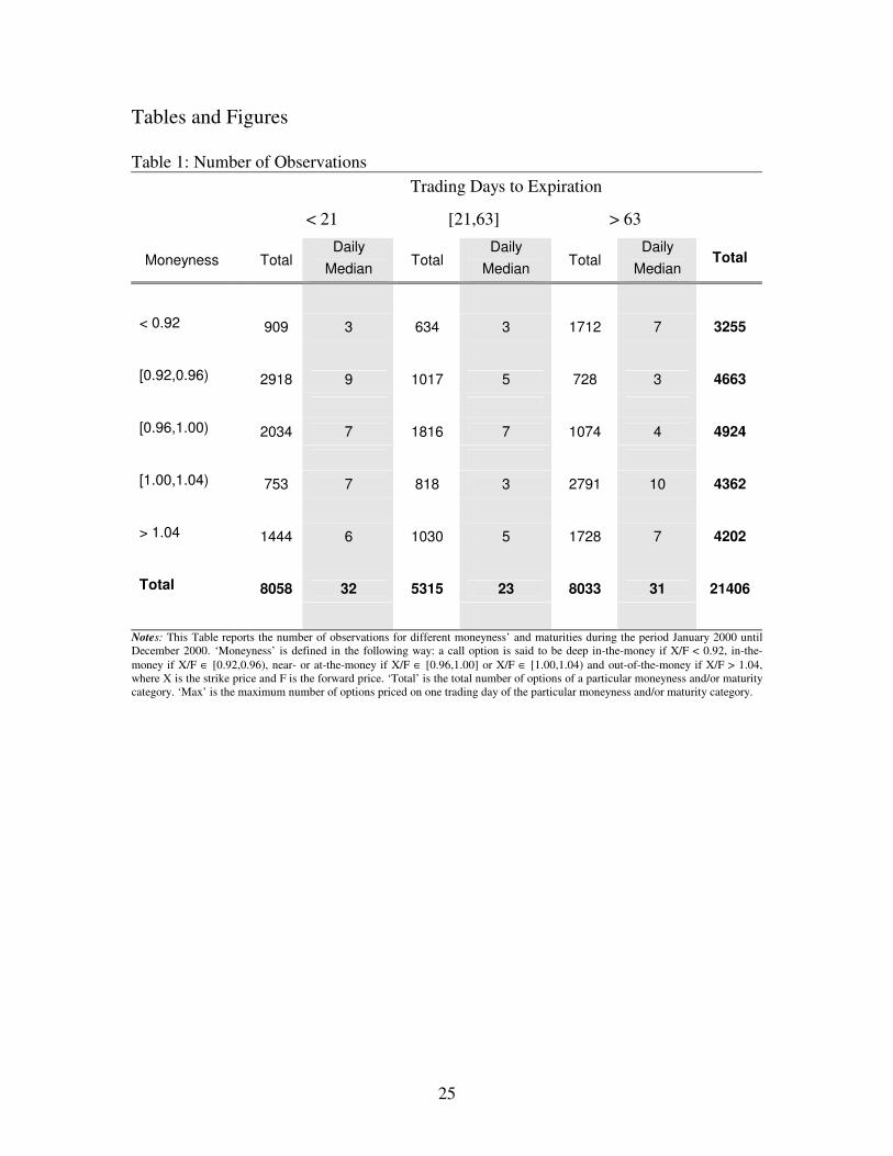
We exclude options with less than one week and more than 25 weeks until
maturity and options with a price of less than 2 Euro to avoid liquidity-related biases and
because of less useful information on volatilities. We filter the available option prices and
include all options that are actively traded, inside or outside the 10% absolute moneyness
interval. In practice, in volatile periods deep out-of-the money options are highly
informative if they are actively traded. As a result, each day we use a minimum of 3, but
typically 4 different maturities for the calibration.
_____________________
Insert Table 1 Here
_____________________

11
The DAX index calculation is based on the assumption that the cash dividend payments
are reinvested. Therefore, when calculating option prices, theoretically we do not have to
adjust the index level for the fact that the stock price drops on the ex-dividend date. But
the cash dividend payments are taxed and the reinvestment does not fully compensate for
the decrease in the stock price. Therefore, in the conversion from e.g. futures prices to the
implied spot rate, one empirically observes a different implied dividend adjusted
underlying for different maturities. For this reason, we work with the adjusted underlying
index level implied out from futures or option market prices.
In a nutshell, the option pricing procedure boils down the following. First of all,
the dividend adjusted value for the underlying is determined for a certain day; in our case,
that is the DAX30 on January 1st 2000. Next, a set of options is observed with different
times to maturity and different strikes for that same day. Using Monte Carlo simulations,
the model generates a certain forecasts for all the different expiration dates. In other
words, it starts off from the observed dividend-adjusted underlying of today, and iterates
forward until expiration. Next, option prices are calculated with these forecasts using the
standard Black and Scholes approach, and compared with the empirically observed
option prices. The optimisation procedure then consists of minimizing the root-mean-
squared pricing error of the total set of options per day. The equilibrium set of
coefficients is then used as starting values for the optimization procedure for the next
day. This whole procedure is repeated for each trading day in the dataset. In particular we
are using the following procedure for one particular day to price options on the following
trading day:
First, we compute the implied interest rates and implied dividend adjusted index
rates from the observed put and call option prices. We are using a modified put-call parity
regression proposed by Shimko (1993). The put-call parity for European options reads:
)(
,, )]([tTr
ijtjiji
jjeXDPVSpc−−
−−=− (8)
where ci,j and pi,j are the observed call and put closing prices, respectively, with exercise
prices Xi and maturity (Tj-t), PV(Dj) denotes the present value of dividends to be paid
12
from time t until the maturity of the options contract at time Tj and rj is the continuously
compounded interest rate that matches the maturity of the option contract. Therefore, we
can infer a value for the implied dividend adjusted index for different maturities, St-
PV(Dj), and the continuously compounded interest rate for different maturities, rj. To
ensure that the implied dividend adjusted index value is a non-increasing function of the
maturity of the option, we occasionally adjust the standard put-call parity regression.
Therefore, we control and ensure that the value for St - PV(Dj) is decreasing with
maturity, Tj. Since we are using closing prices for the estimation, one alternative is to use
implied index levels from DAX index futures prices assuming that both markets are
closely integrated.
Second, we estimate the parameters of the particular models by minimizing the
loss function. Parameters of the model are calibrated by minimizing the root mean
squared absolute pricing error between the market prices and the theoretical option
prices:
( )∑∑= =
−=n
i
m
j
jiji
i
ccN
RMSE1 1
2
,,ˆmin
1 (9)
where N is the total number of call options evaluated, the subscript i refers to the n
different maturities and subscript j to the mi different strike prices in a particular maturity
series i.
Given reasonable starting values, we price European call options with exercise
price Xi and maturity Tj. Using well-known optimization methods (e.g. Newton-Raphson
method), we obtain the parameter estimates that minimize the loss function. The
goodness of fit measure for the optimization is the mean squared valuation error criterion.
Third, having estimated the parameters in-sample, we turn to out-of-sample
valuation performance and evaluate how well each day’s estimated models value the
traded options at the end of the following day. We filter the available option prices
according to our criteria for the in-sample calibration. The futures market is the most
liquid market and the options and the futures market are closely integrated, therefore it
can also be assumed that the futures price is more informative for option pricing than just
13
using the value of the index. For every observed futures closing price we can derive the
implied underlying index level and evaluate the option. Given a futures price Fj with time
to maturity Tj, spot futures parity is used to determine St-PV(Dj) from
jjT-re)(S jjt FDPV =− (10)
where PV(Dj) denotes the present value of dividends to be paid from time t until the
maturity of the options contract at time Tj and rj is the continuously compounded interest
rate (the interpolated EURIBOR rate) that matches the maturity of the futures contract (or
time to expiration of the option). If a given option price observation corresponds to an
option that expires at the time of delivery of a futures contract, then the price of the
futures contract can be used to determine the quantity St-PV(Dj) directly.
The maturities of DAX index options do not always correspond to the delivery
dates of the futures contracts. In particular for index options the two following months
are always expiration months, but not necessarily a delivery month for the futures
contract. When an option expires on a date other than the delivery date of the futures
contract, then the quantity St-PV(Dj) is computed from various futures contracts. Let F1
be the futures price for a contract with the shortest maturity, T1 and F2 and F3 are the
futures prices for contracts with the second and third closest delivery months, T2 and T3,
respectively. Then the expected future rate of dividend payment d can be computed via
spot-futures parity by:
)TT(
)F/F(logTrTrd
23
232233
−
−−= (11)
Hence, the quantity St-PV(D) = Ste–dT
associated with the option that expires at time T in
the future can be computed by6
))((
111 dTTdrdT
t eFeS−−−− = . (12)
6 See e.g. the appendix in Poteshman (2001) for details.

14
This method allows us to perfectly match the observed option price and the underlying
dividend adjusted spot rate. Given the parameter estimates and the implied dividend
adjusted underlying we can calculate option prices and compare them to the observed
option prices of traded index options. For the out-of-sample part the same loss functions
for call options are used. The prediction performance of the various models are evaluated
and compared by using the root mean squared valuation error criterion. We compare the
predicted option values with the observed prices for every traded option. We repeat the
whole procedure over the out-of-sample period and conclude, which model minimizes the
out-of-sample pricing error.
In order to evaluate options, the physical process has to be transformed to a risk-
neutral process. We make use of the Local Risk Neutral Valuation Relationship
(LRNVR) developed in Duan (1995). Under the LRNVR the conditional variance
remains unchanged, but under the pricing measure Q the conditional expectation of rt is
equal to the risk free rate rf :
[ ] )exp()exp( 1 ftt
QrrE =Ω − , (13)
The risk-neutral Gaussian process reads:
tttf
ttt
ttt hr
DPVS
DPVSr εσ +−=
−
−=
−−
2
21
11 )(
)(ln ,
)1,0(~| 1 Ntt −Ωε under the risk-neutralized probability measure Q
(14)
In Equation (14), tε is not necessarily normal, but to include the Black-Scholes model as
a special case we typically assume that tε is a Gaussian random variable. The locally
risk-neutral valuation relationship ensures that under the risk neutral measure Q, the
volatility process satisfies

15
[ ] [ ] ttt
P
tt
QhrVarrVar =Ω=Ω −− 11 . (15)
A European call option with exercise price X and time to maturity T has at time t
price equal to:
( ) ( )[ ]1|0,maxexp −Ω−−= tt
Q
tt XSErTc (16)
For this kind of derivative valuation models with a high degree of path dependency,
computationally demanding Monte Carlo simulations are commonly used for valuing
derivative securities. We use the recently proposed simulation adjustment method, the
empirical martingale simulation (EMS) of Duan and Simonato (1998), which has been
shown to substantially accelerate the convergence of Monte Carlo price estimates and to
reduce the so called ‘simulation error’.
In the empirical part of the paper, we model the expectations of conditional
volatility of fundamentalists (and chartists) in an EGARCH setting, which is motivated
by the empirical data fitting (see Lehnert (2003)). Applying a standard GARCH
framework resulted in numerous violations of parameters in their permissible parameter
space. The EGARCH setting resolves these issues, as it imposes no restrictions on the
parameter space (see Nelson, 1991).
5. Results
This section presents the empirical results of the option pricing application of our
heterogeneous agents model for the second moment. First, we present one specific path
from the Monte Carlo simulations in order to gain somewhat more feeling on the
behaviour of the proposed model. Second we focus on both the estimation results and the
stability of the estimates through time. Finally, we look at the pricing errors of our model,
both in-sample and out-of-sample. The estimation exercises are conducted in a setting
with and without switching. This allows us to examine the direct effect of introducing
more flexibility in the model; in other words, it allows us to see the advantage of our
model over a standard GARCH.

16
_______________________
Insert Figure 1 Here
_______________________
Figure 1 presents a close-up of a one simulation path out of 10.000 in the Monte Carlo
setup; it uses the (optimized) coefficients from a random day, May 5th
in this case7. A
number of observations can be made. As one would expect, the volatility h lies between
the expectations of the fundamentalists hF and chartists h
C. The distance between the
three is governed by the weight wt. Weights fluctuate continuously around the benchmark
of one half with a minimum of 0.14 and maximum of 0.81. The nature of the two groups
is clearly illustrated by the course of the volatility process. High spikes in volatility
always coincide with low weights; i.e., a relatively high volatility is caused by the fact
that the market is dominated by chartists. The most clear example of this can be seen
around observation number 40 where w reaches its minimum and h its maximum. The
reverse is true as well; when fundamentalist make up over 80% of the market around
period 70, volatility drops towards its long-run value. Therefore, fundamentalists are
stabilizing, and chartists destabilizing. None of the groups gets driven out of the market,
and both groups experience periods of dominance.
_______________________
Insert Table 2 Here
_______________________
7 The coefficients are given by α=-0.087; β0=-0.365; β1=0.337; and γ=40.450.

17
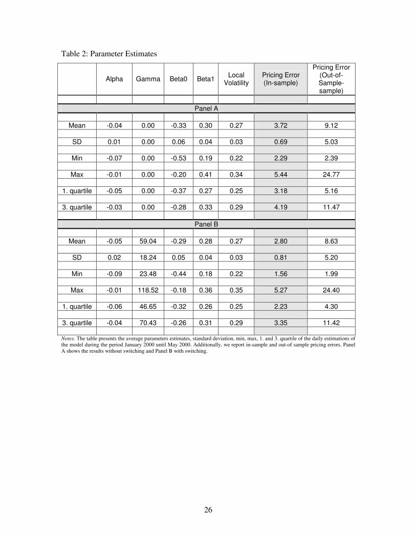
Table 2 presents the estimation results of the option pricing application of the
heterogeneous agents model; the distributional characteristics of the estimates over time
are depicted. Overall, we observe that all coefficients have the sign and magnitude as
hypothesized by the model. Both fundamentalists and chartists appear to be active on the
market; their individual effects on the variance process are as expected (stabilizing and
destabilizing, respectively). Also, we find significant evidence of switching between the
two rules.
Focusing on the static setup first (Panel A); the mean-reversion parameter α is
negative throughout the sample, implying that fundamentalists consistently apply a
stabilizing expectation formation rule. They therefore introduce a mean reverting
dynamics into the variance process, as they expect the variance to return to the long run
volatility. The absolute magnitude of the mean estimate of α indicates that
fundamentalists expect on average 4% of the excess volatility to disappear in the next
period. The average estimated local volatility, i.e. the starting value for the volatility
dynamics, is estimated to be equal to 27% (annualized), which is very much in line with
the time series volatility of the DAX index in that period.
Parameter estimates for the chartist expectation formation rule in the model, β0
and β1, have the expected sign as well. The results for this asymmetric setup imply that
there is a clear leverage effect: Positive shocks in the level result in a reduction of the
variance β0<0; negative shocks in the level result in an increase of the variance β1>0.
Therefore, negative shocks in the level have a destabilizing effect to the variance process
because of the chartists’ expectation formation rule.
The results for the switching setup, in Panel B, are generally consistent with the
static setup. The difference, the sensitivity of choice parameter γ, is positive throughout
the sample. This implies that the switching mechanism functions as a positive feedback
rule. In other words, the positive sign of the coefficient indicates that agents switch
towards the group with the smallest forecasting error. The magnitude of γ is conditional
on the functional form of the profit function (in our case, a loss function consisting of the
percentage forecasting error). Therefore, it is not possible to make any statements about
the sensitivity to profit differences of traders in the option market at this time. We will,
18
however, be able to say something about the evolution of individual’s behaviour over
time in the sensitivity analysis below.
As additional empirical evidence for our model, we examined both the in-sample
and out-of-sample pricing errors. The results for the models with and without switching
are depicted in the final two columns of Table 2. Results suggest that the assumption that
agents always switch to the more profitable forecasting rule is very much supported by
the data. Comparing Panel A and B reveals that our most sophisticated model
outperforms the benchmark with on average € 0.92 for the in-sample and € 0.49 for the
out-of-sample pricing error. In other words, next to introducing a more intuitive appeal to
volatility models, our heterogeneous agents setup for the second moment also proves to
be more effective in explaining and forecasting option prices.
To our best knowledge, a heterogeneous agents model has never been applied to
the options market. We can, however, compare our results with related literature. First of
all, the signs and magnitudes of the chartist expectation formation function are directly
comparable to the standard EGARCH-results, due to Nelson (1991). The relative impact
of positive versus negative shocks corroborates previous findings; the typical results for
the leverage effect indicate that the relative effect of negative shocks on the variance
process is larger than the positive shocks. Second, our results are directly in line with
previous findings on estimates of heterogeneous agents models for alternative markets.
Boswijk et al. (2007) find significant evidence of the co-existence of chartists and
fundamentalist for the S&P500 from 1870 to 2006; De Jong et al. (2007) present similar
results for the British Pound during the EMS crisis. Our results on the switching
mechanism, however, are stronger compared to Boswijk et al. (2007) and De Jong et al.
(2007); evidence for switching is limited given their estimate of the switching parameter.
This implies that traders in the options market are more prone to change their strategy in
response to a difference in profits compared to traders in the S&P500 or foreign exchange
market.
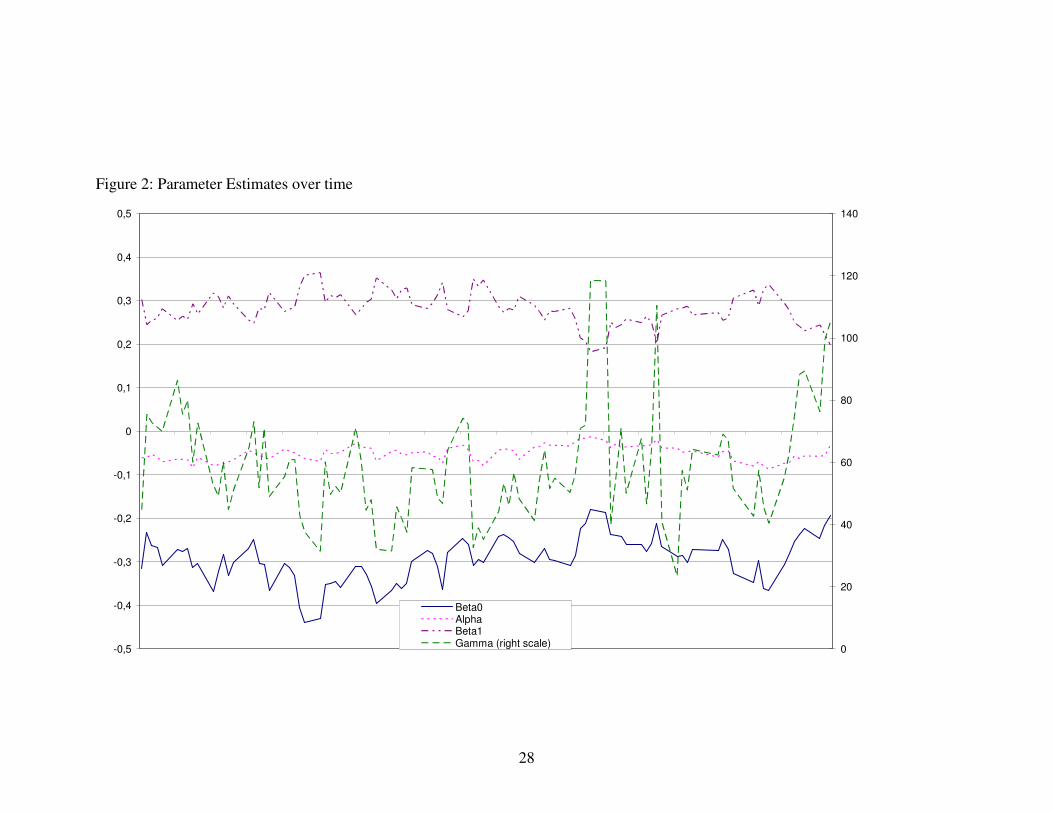
Given that the model is estimated for different maturities and levels of moneyness
for each day of the year, we can examine the stability of the estimated coefficients during
the estimation process. By following the evolution of the estimated coefficients, we will
19
be able to say something about the conditional behaviour of heterogeneous traders.
Figure 2 depicts the development of the coefficient estimates over time.
______________________
Insert Figure 2 Here
______________________
Figure 2 displays the development of the two expectation formation functions,
fundamentalists and chartists, and the intensity of choice parameter. Overall, the
parameters of the fundamentalist and chartist expectation formation functions are
relatively stable; α, β0 and β1 move in a relative small band within the region you expect
them to be.
At around two-thirds of the sample α, β0 and β1 start moving towards zero, while γ
becomes larger and more volatile. This evolution of the parameters can be directly
explained by the logic of the underlying heterogeneous agents model. Apparently, the
volatility in the underlying is relatively constant in this middle period, which can be seen
from the fact that the coefficients of the expectation formation functions go to zero. Both
groups form their expectation as the most recently observed volatility, plus some
correction term; as the correction term goes to zero, agents expect a constant volatility.
As both fundamentalists and chartists expect small innovations to the volatility process,
the profit difference between the two strategies as well as the forecasting error itself will
be small. As the forecasting errors are small, large shifts in γ will not induce large shifts
in the distribution of weights over strategies (see Equation 4). This is exactly why the
estimate of γ shows large shifts in this period.
_________________________
Insert Figure 3 Here

20
_________________________
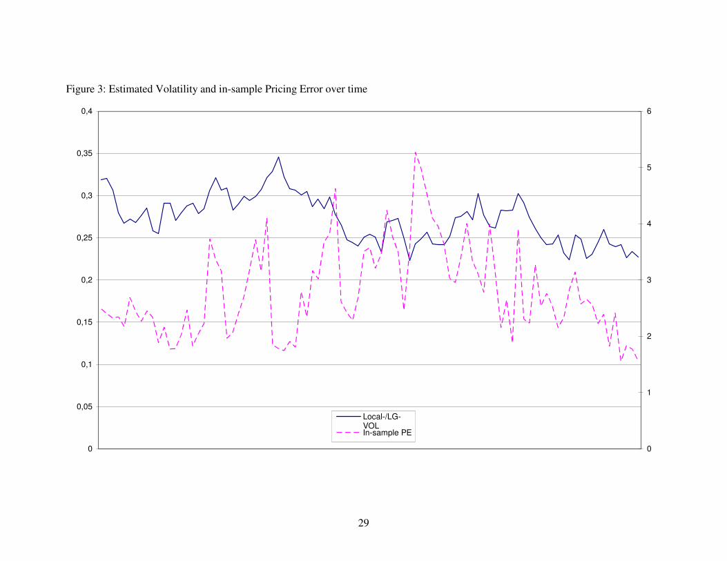
Figure 3 presents the evolution of the estimated local volatility and the in-sample pricing
error of our model. There is a clear positive correlation between the estimated
fundamental volatility and the pricing error. Consistent with previous literature, we find
that volatility shows distinctive periods of high and low volatility. Interestingly, the local
volatility estimates exactly fluctuate around the long-run volatility level estimated from
return data.
6. Conclusions
In this paper we introduce a model of behavioral volatility trading. Being the only
unobserved variable in an option pricing model, volatility plays a pivotal role in the
determination of the value of an option. Our market consists of two types of agents that
have different views on volatility and trade accordingly. Fundamentalists are expecting
the conditional volatility to mean revert to a long-run volatility level. Chartists on the
other hand respond solely on noise from the level process and bid up (down) volatility if
they receive a negative (positive) signal from the stock market. Depending on the
profitability of their strategy, agents are able to switch between groups according to a
multinomial logit switching mechanism. The model is shown to reduce to a GJR-
GARCH(1,1) with time varying coefficients. The difference, however, lies in the fact that
we provide a behavioral underpinning; also, time variation in the coefficients is
dependent on trader behavior.
In an application of the model to DAX index options, using the GARCH option
pricing model, we find evidence that different types of traders are actively involved in
trading volatility. Both fundamentalists and chartists are shown to be active in the options
markets, and both groups are consistently present. Hence, we find evidence that observed
option prices are the result of heterogeneity in expectations about future volatility. Also,
we find evidence of switching between the groups; that is, at certain points in time the
market is dominated by mean-reverting fundamentalists, at other points by destabilizing
chartists. Introducing the possibility to switch gives a substantial reduction in both in- and
21
out-of-sample pricing errors. In other words, volatility traders indeed change their
forecasting behavior dependent on the relative profitability.
Extensions to the current results are both possible and necessary. Our current
dataset only comprises of call-options for a limited time span. More data will obviously
yield more confidence in the results. The estimation procedure as it is now estimates the
model daily; using the data as a panel, so using both the time-series as the cross-sectional
variation, would make it possible to construct standard errors around the estimates.
It would also be interesting to experiment with alternative specifications of the
model. Think of alternative profit functions, as is common in the heterogeneous agents
literature. Also, the expectation formation functions are flexible to incorporate numerous
different specifications, including ones with exogenous information.

22
References
Avromov, D., T. Chordia and A. Goyal (2006). The Impact of Trades on Daily Volatility,
Review of Financial Studies 19: 1241-1277.
Barberis, N., A. Shleifer, and R. Vishny (1998). A Model of Investor Sentiment, Journal
of Financial Economics 49: 307-343.
Boswijk, H.P., C.H. Hommes and S. Manzan (2007). Behavioral Heterogeneity in Stock
Prices, Journal of Economic Dynamics and Control, forthcoming.
Brock, W. and C. Hommes (1997). A Rational Route to Randomness, Econometrica 69:
1059-1095.
Brock W. and C. Hommes (1998). Heterogeneous Beliefs and Routes to Chaos in a
Simple Asset Pricing Model, Journal of Economic Dynamics and Control 22: 1235-1274.
Carr, P. and D. Madan (2002). Towards a Theory of Volatility Trading. NYU Working
Paper.
Christoffersen, P. and K. Jacobs (2004). Which GARCH Model for Option Valuation?,
Management Science 50: 1204-1221.
De Long, J.B., A. Shleifer, L.H. Summers, and R.J. Waldmann (1990). Noise trader risk
in Financial markets, Journal of Political Finance 98: 703-738.
Duan, J.-C. and J.-G. Simonato (1998), ”Empirical Martingale Simulation for Asset
Prices”, Management Science 44, 1218-1233.
Duan, J.-C. (1995), ”The GARCH Option Pricing Model”, Mathematical Finance 5, 13-
32.
Engle, R. and G. Lee (1999). A Permanent and Transitory Component Model of Stock
Return Volatility, In: Engle, R. and H. White (eds.), Cointegration, Causality, and
Forecasting: A Festschrift in Honour of Clive W.J. Granger. Oxford University Press,
pp. 475-497.
Hommes, C.H. (2006). Heterogeneous Agents Models in Economics and Finance, In:
Tesfatsion, L. and Judd, K.L. (eds.), Handbook of Computational Economics, Volume 2:
Agent-Based Computational Economics, Elsevier Science.
Fama, E. (1971). Risk, Return, and Equilibrium, Journal of Political Economy 79(1):30-
55.
23
Frankel, J.A. and Froot, K.A. (1986). Understanding the US Dollar in the Eighties: The
Expectations of Chartists and Fundamentalists, Economic Record, 62(supplement): 24-
38.
Frankel, J.A. and Froot, K.A. (1990). Chartists, Fundamentalists, and Trading in the
Foreign Exchange Market, American Economic Review, 80(2):181-185.
Frijns, B., Koellen, E. and T. Lehnert (2008). On the Determinants of Portfolio Choice,
Journal of Economic Behavior and Organization (forthcoming).
Glosten L., R. Jagannathan and D. Runkle (1993). Relationship between the Expected
Value and the Volatility of the Nominal Excess Return on Stocks, Journal of Finance,
48: 1779-1801.
Grauwe, De. P. and M. Grimaldi (2005). Heterogeneity of Agents, Transaction Costs and
the Exchange Rate, Journal of Economic Dynamics and Control 29: 691-719.
Grauwe, De. P. and M. Grimaldi (2006). Exchange Rate Puzzles: A Tale of Switching
Attractors, European Economic Review 50(1): 1-33.
Guo, C. (1998). Option Pricing with Heterogeneous Expectations, The Financial Review
33: 81-92.
De Jong, E., W. Verschoor and R. Zwinkels (2007). A Heterogeneous Route to the EMS
Crisis, Applied Economics Letters (forthcoming).
Kahneman, D., and A. Tversky (1979). Prospect Theory: An Analysis of Decision under
Risk, Econometrica, XVLII: 263–291.
Kurz, M. (1994). On the Structure and Diversity of Rational Beliefs, Economic Theory,
4(6): 877-900.
LeBaron, B., W.B. Arthur and R. Palmer (1999). Time Series Properties of an Artificial
Stock Market, Journal of Economic Dynamics and Control 23: 1487-1516.
Lee, W. Y., Jiang, C. X. and Indro, D.C. (2002), “Stock market volatility, excess returns,
and the role of investor sentiment,” Journal of Banking and Finance, Vol. 26, pp. 2277-
2299.
Lehnert, T. (2003)”, “Explaining Smiles: GARCH Option Pricing with Conditional
Leptokurtosis and Skewness, Journal of Derivatives 10, 3, 27-39.
Lux, T. (1998). The Socio-Economic Dynamics of Speculative Markets: Interacting
Agents, Chaos and the Fat Tails of Return Distribution. Journal of Economic Behavior
and Organization 33: 143-165.
24
MacDonald, R. (2000). Expectations Formation Risk in Three Financial Markets:
Surveying what the Surveys Say, Journal of Economic Surveys 14(1): 69-100.
Milgrom, P. and N. Stokey (1982). Information, Trade, and Common Knowledge,
Journal of Economic Theory 26(1): 17-27.
Muth, J.F. (1961). Rational Expectations and the Theory of Price Movements,
Econometrica, 29(3): 315-335.
Nelson, D.B., 1991, Conditional Heteroskedasticity in Asset Returns: A New Approach,
Econometrica 59(2):347-370.
Poteshman, A.M. (2001), “Underreaction, Overreaction, and Increasing Misreaction to
Information in the Option Market”, Journal of Finance 56, 3, 851-876.
Reitz, S. and F.H. Westerhoff (2003). Nonlinearities and Cyclical Behavior: the Role of
Chartists and Fundamentalists. Studies in Nonlinear Dynamics and Econometrics 7(4), 3.
Reitz, S. and F. Westerhoff (2006): Commodity price cycles and heterogeneous
speculators: A STAR-GARCH model. Empirical Economics, in press.
Reitz, S. and F. Westerhoff. (2005): Commodity price dynamics and the nonlinear market
impact of technical traders: empirical evidence for the U.S. corn market. Physica A:
Statistical Mechanics and its Application 349: 641-648.
Ziegler, A. (2002). State-price Densities under Heterogeneous Beliefs, the Smile-Effect,
and Implied Risk Aversion. European Economic Review 46: 1539-1557.
25
Tables and Figures
Table 1: Number of Observations
Trading Days to Expiration
< 21 [21,63] > 63
Moneyness Total Daily
Median Total
Daily
Median Total
Daily
Median Total
< 0.92 909 3 634 3 1712 7 3255
[0.92,0.96) 2918 9 1017 5 728 3 4663
[0.96,1.00) 2034 7 1816 7 1074 4 4924
[1.00,1.04) 753 7 818 3 2791 10 4362
> 1.04 1444 6 1030 5 1728 7 4202
Total 8058 32 5315 23 8033 31 21406
Notes: This Table reports the number of observations for different moneyness’ and maturities during the period January 2000 until
December 2000. ‘Moneyness’ is defined in the following way: a call option is said to be deep in-the-money if X/F < 0.92, in-the-
money if X/F ∈ [0.92,0.96), near- or at-the-money if X/F ∈ [0.96,1.00] or X/F ∈ [1.00,1.04) and out-of-the-money if X/F > 1.04,
where X is the strike price and F is the forward price. ‘Total’ is the total number of options of a particular moneyness and/or maturity
category. ‘Max’ is the maximum number of options priced on one trading day of the particular moneyness and/or maturity category.
26
Table 2: Parameter Estimates
Alpha Gamma Beta0 Beta1 Local
Volatility Pricing Error (In-sample)
Pricing Error (Out-of-Sample-sample)
Panel A
Mean -0.04 0.00 -0.33 0.30 0.27 3.72 9.12
SD 0.01 0.00 0.06 0.04 0.03 0.69 5.03
Min -0.07 0.00 -0.53 0.19 0.22 2.29 2.39
Max -0.01 0.00 -0.20 0.41 0.34 5.44 24.77
1. quartile -0.05 0.00 -0.37 0.27 0.25 3.18 5.16
3. quartile -0.03 0.00 -0.28 0.33 0.29 4.19 11.47
Panel B
Mean -0.05 59.04 -0.29 0.28 0.27 2.80 8.63
SD 0.02 18.24 0.05 0.04 0.03 0.81 5.20
Min -0.09 23.48 -0.44 0.18 0.22 1.56 1.99
Max -0.01 118.52 -0.18 0.36 0.35 5.27 24.40
1. quartile -0.06 46.65 -0.32 0.26 0.25 2.23 4.30
3. quartile -0.04 70.43 -0.26 0.31 0.29 3.35 11.42
Notes. The table presents the average parameters estimates, standard deviation, min, max, 1. and 3. quartile of the daily estimations of
the model during the period January 2000 until May 2000. Additionally, we report in-sample and out-of sample pricing errors. Panel
A shows the results without switching and Panel B with switching.
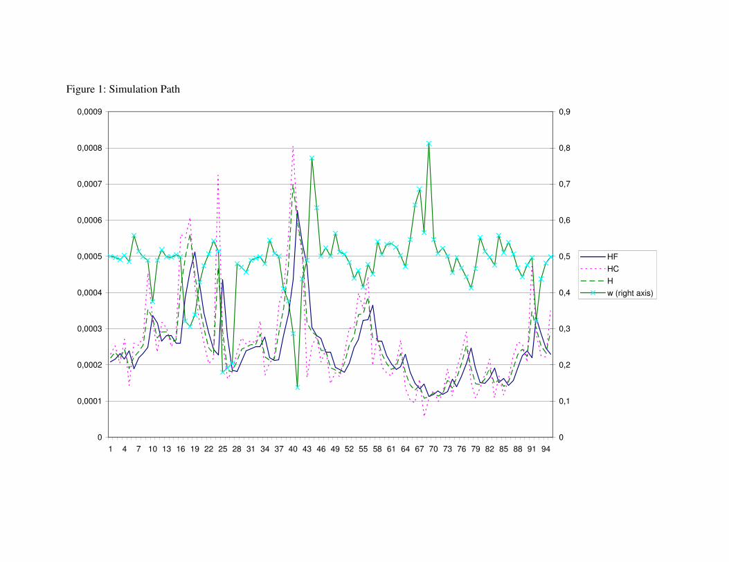
Figure 1: Simulation Path
0
0,0001
0,0002
0,0003
0,0004
0,0005
0,0006
0,0007
0,0008
0,0009
1 4 7 10 13 16 19 22 25 28 31 34 37 40 43 46 49 52 55 58 61 64 67 70 73 76 79 82 85 88 91 94
0
0,1
0,2
0,3
0,4
0,5
0,6
0,7
0,8
0,9
HF
HC
H
w (right axis)
28
Figure 2: Parameter Estimates over time
-0,5
-0,4
-0,3
-0,2
-0,1
0
0,1
0,2
0,3
0,4
0,5
0
20
40
60
80
100
120
140
Beta0AlphaBeta1Gamma (right scale)
29
Figure 3: Estimated Volatility and in-sample Pricing Error over time
0
0,05
0,1
0,15
0,2
0,25
0,3
0,35
0,4
0
1
2
3
4
5
6
Local-/LG-VOLIn-sample PE