L

AA ~ .. ~----------------------------------------

AIAA-2003-3975 On a Non-Reflecting Boundary Condition for Hyperbolic Conservation Laws Ching Y. Loh Taitech, Inc. Beaver Creek, OH

16th AIAA Computational Fluid Dynamics Conference and the 33rd Fluid Dynamics Conference and Exhibit

June 23-26, 2003 / Orlando, FL

For permission to copy or republish, contact the American Institute of Aeronautics and Astronautics 1801 Alexander Bell Drive, Suite 500, Reston, VA 20191-4344

____ ___ J

https://ntrs.nasa.gov/search.jsp?R=20150012266 2019-05-28T13:37:45+00:00Z

I~

ON A NON-REFLECTING BOUNDARY CONDITION FOR HYPERBOLIC CONSERVATION LAWS

Ching Y. Loh* Taitech Inc.

Beaver Creek, Ohio 44135,U8 A

Abstract A non-refl ecting boundary condition (NRBC) fo r practical computati ons in fluid dynamics and aeroacousti cs is presented. The technique is based on the hyperbolic ity of the Euler equa­ti on system and the first principle of pl ane (s imple) wave propagati on [1] . The NRBC is s imple and effec tive, provided the numerical scheme maintains locall y a C 1 continuous so­lution at the bounda ry. Several numerical ex­amples in ID, 2D and 3D space are illustrated to demonstrate its ro bustness in practical com­putati ons.

1 Introduction It is well -known that non-refl ecting boundary con­

di tio ns (NRBCs) play a n important role in fluid fl ow and aeroacousti cs computati ons. The need fo r arti fi cial boundary conditions ari ses when the domain of the prob­lem is unbounded and ex tends to infinity. In order to treat the problem numericall y, a domain of finite s ize is required and artificial boundari es are imposed. A t these artificia l boundaries , NRBCs are sought for to minimize their influences on the fl ow. A spurious re fl ecti on result­ing from an inappropriate numerical boundary condition will contaminate the fl ow fi eld and may entire ly spoil the fl ow computation. Research on NRBC is a challeng­ing topic in e ng ineering and applied mathematics. For decades, a vast number of papers on NRBC have been published, e.g. see [3-6], the rev iew paper by Gi vo li [2], and the references cited there .

In one-dimensional fl ow, at an artific ial boundary, E n­qui st and Majda [3], and Hedstrom [7] proved that a boundary condition is non-re fl ecting is equi vale nt to say­ing that the characteri sti c vari ables corresponding to the incoming characteristi c c urve remain constant across the artifi cia l boundary (see also Hirsch [8], p. 370). For multi-dime nsional fl ow, thi s I -D technique is combined with d imension spli tting and applied in the practi ca l

NRBC treatme nt. Such a combined treatment has been the topic of many papers on the characteristic based NR­BCs (see e.g. [4] and references in [2]) .

Other alternative treatments for NRBC found in the literature inc lude (see [2-6]):

(i) in the far- fi eld , using a predictable asy mptotic a na­lyti ca l solution at the boundary ( the radi ati on boundary condition),

(ii ) diminishing the stre ngth of the waves/di sturbances before they reach the arti fic ial boundary, and thus mini ­mi zing the refl ecting effect. Usuall y, increased nume ri­cal damping is applied to a zone between the core domain and the arti fic ia l boundary (the buffer zone or sponge zone) to do the job. In the recentl y developed PML (pe r­fec tl y matched layer) method, a spec iall y des igned equa­ti on system is imposed in the matching layer (or sponge zone) to guarantee the exponenti al decay ing of the di s­turbances in the layer [5,6].

In the present paper, a di fferent but simple criteri on is in troduced to treat the NRBCs of the time-dependent hyperbolic conservati on laws of gas dynamics. T he c ri ­teri on is based on the first principl e of plane (simple) wave propagati on [1] rather than the characteri stics the­ory. Emphas is is put on the ir viable practical applica­tions. As it turns out that the NRBCs used in the recent CE/SE finite volume schemes fo r fl ow and aeroacous­tics computatio ns (e.g. [ 14 , 15]) can be directl y derived from thi s criteri on, the present paper also serves to ex­plain why these simple NRBCs of the CE/SE schemes work .

The paper is arranged as fo llows: In Secti on 2 , based on the hyperbolicity of the Euler equation system and the propagati on of plane wave, the continui ty cri teri on of NRBC is introduced and proved. An extrapo lati on­li ke NRBC (Type I) based on thi s criteri on and the nu­merical procedure are described. Then the relati on be­tween the NRBC and the flu x balance across the bound­ary surface is establi shed, which leads to another type of NRBC (Type II). In Section 3, several numeri cal ex-

American Institu te of Aeronautics and Astronautics

-

I

L

amples for outfl ow NRBC in one and mu lti-dimens ional space are presented. Numerica l examples with Type II NRBC at the inflow and other artificial boundaries are demo nstrated in Section 4. Applicati on of buffer/sponge ones is illustrated in Section 5. At last, the paper is con­

cluded with remarks in Section 6.

As the time-dependent hyperbo lic conservati on laws of gas dynamics ( in d imensionless fo rm) is a lways in ­corporated in the new trea tments of NRBC in the present pape r, they are brie fl y described here for later use:

Ut+ F x+ G y +Hz = Q , ( I )

where x, y, z and t are the streamwise and transversal co­ordinates and time, respecti vely. The conservative fl ow variable vector U and the flux vectors in the streamwise and radi al directi ons, F , G , and H , are g iven by:

( Ul ) ( P) (Fl ) ( pu ) U2 pu F2 pu 2 + P

U = g: = :: ' F = ~: = :: U5 pe F5 puH

G ~ (g: ) ~ (;: p } G4 pvw G5 pvH

H ~ (~ ) ~ ( :: ) H 4 pw2 + P H 5 pwH

where u , v, wand p, p are respectively the veloc ity com­

pone nts, density and pressure, e = p(-t- l ) + 1/ 2(u2 + v2 + w2

), and the enthalpy H = pi p + e with "f = 1.4. The right hand side Q is the source term which may in­clude the poss ible external forc ing terms and/or viscous fluxes.

By considering (x,y, z, t) as coordinates of a four­dime nsio nal E uclidean space, E 4 , and using Gauss 's di­vergence theorem, it fo llows that Eq. ( 1) is equi valent to the following integral conservati on laws:

1 1m . ds = r Qmd V, Ts(v) Jv

m = 1, 2,3,4, 5, (2)

where S(V) denotes the surface around a volume V in E4 and 1m = (Fm , Gm, Hm, Urn) stands for the flu x vectors, 1mds = 1m • n d8 , n be ing the outgo ing unit normal vector in E4 , is the flu x at the infinitesima l sur­face ele ment d8 .

2

boundary surface element L'l.s inner side \ outer

P;-<> Pe--o

.~

x computational domain

Figure 1: The NRBC criterio n in E3 .

2 The continuity criterion of NRBC for time dependent conservation laws

There are various techn iques to treat the NRBC based on characteri sti cs theory o f the hyperboli c sys tem. For instance, a we ll-known I -D fl ow NRBC treatme nt by E n­qui st and Majda [3], and Hedstrom [7] is the require me nt that the loca l pe rturbati on (di sturbance) along incoming characteristics be made va ni sh at the boundary (see [8], p.370). Let W = (Wl ,W2, W3)T be the 1-0 c haracter­istic fl ow variables, the above require ment states that for those k such that the corresponding characteristic enters the computa ti onal domain through the artific ia l bo und­ary:

6.Wk = 0 (3)

Tho mpson [4] , for example, has detail s on the prac ti cal impleme ntati on of the characteri stic NRBCs with a finite difference sche me. Hirsch [8] also offers an excell e nt resource of vario us NRBCs.

In finite vo lume numeri cal approaches with hyperbolic conservati on laws, grid nodes are ofte n ce ll centers and the boundary faces are ofte n formed by the boundary cell surfaces. No node lies exactly on the boundary. As such, a continuity crite ri on o fNRBC a nd the consequent NRBC treatme nts are recomme nded based on the hy­perbolic ity of the equati o n system and the first princ iple of plane wave propagati on [1]. They are s imple, robust and particul arly appropria te for cell center finite vo lume schemes. Their limitati ons are also brie fl y di scussed.

2.1 The continuity criterion of NRBC The continui ty crite ri on is first introduced in an heuri stic way and then proved via the first princ iple of pl ane wave propagati on [I].

Under a general assumption that the fl ow is continu­ous near the boundary, i.e., with no shock or contac t di s­continuity, we first consider the behav ior of the charac­te ri stic variables W = (Wl, W2 , W3 , W4 , W5) T across the artifi cial boundary surface ele ment 6.8 as time elapses. 6.8 also represents the interface between a boundary cell

Ameri can Institute of Aeronautics and Astronautics

I

L __

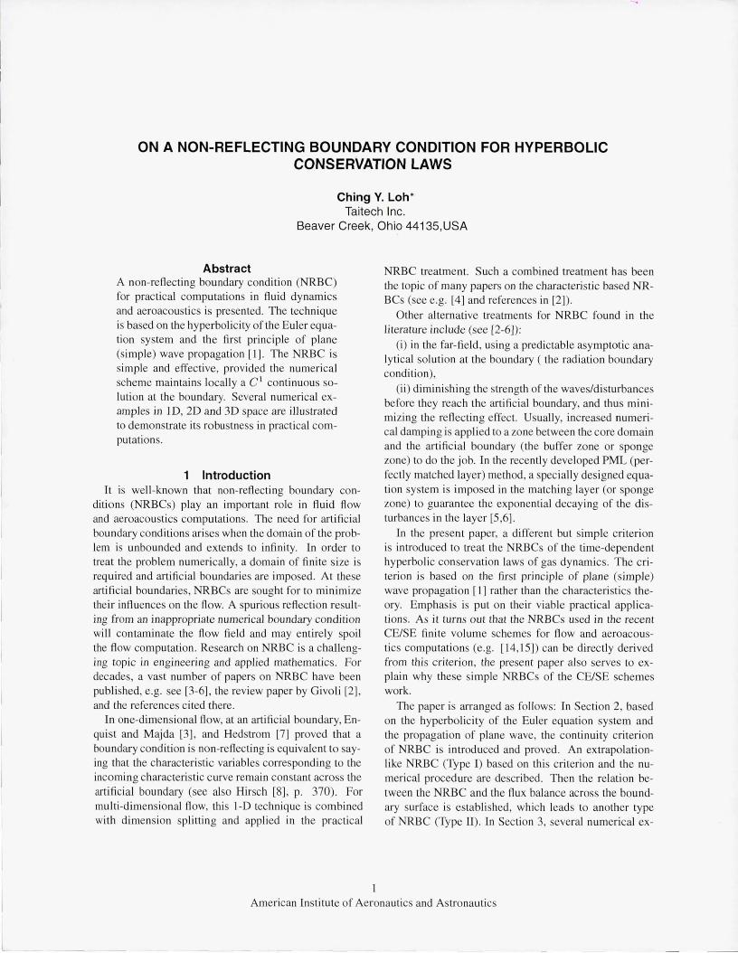
and its corresponding ghost cell. Note that any (artifi ­cial) spatial boundary is a cylindrica l hyper-surface in the space-time E4 space (Fig. 1 demonstrates the s ituation in

E3)' Let Pi and Pe be respectively an interi or poi nt and

an exteri or point of the computat ional domain in the E4 space. Both Pi and Pe li e in the neighborhood of 0 , a poi nt on 6.. s (Fig. I ). Recall the standard NRBC treat­ment for J-D fl ow [3,7] ,

!1Wk = Wk( Pi ) - Wk( Pe ) = 0, for selected k.

Whe n Pi tends to 0 from the interior of the doma in and Pe tends to 0 from the exteri or of the domain , the NRBC Eq. (3) becomes:

lim Wk(Pi ) = lim Wk(Pe ) = Wk(O) (4) Pi--+O Pe--+O

for those selected ks. Therefore, the usual NRBC treat­ment is form ally interpre ted as a continuity problem of Wk across the boundary surface.

Secondly, for the NRBC of multi-dime nsional fl ow, we forma ll y ex tend the continui ty of Wk across the boundary surface to all ks rather than just a selected num­ber of ks:

lim Wk(Pi ) = lim Wk(Pe ), f or all k. (5) Pi--+O Pe--+O

Let U = (Ul ,U2 ,U3,U4,US)T = (p,pu,pv,pw,pe)T and V = (V! ,V2,V3,V4,V5)T = (p ,u ,v,w, p)T be re­specti ve ly the conservative fl ow variab les and the prim­itive flow variables. From the local equi valence of the characteri stic variables W and V or U (see e.g. Hirsch[8] , p.155- I 56), Eq. (5) is equi valent to the conti­nuity of V or U across the artific ial boundary surface:

lim Uk(Pi ) = lim Uk(Pe ), f or all k (6) Pi --+O Pe--+O

or

lim Vk(Pi ) = lim Vk(Pe ), for all k (7) Pi --+0 Pe --+O

It is advantageous to sw itch from the continuity re lation (5) of W to that of V o r U , (6) or (7), s ince the latter can be treated in an easy way. At this stage, the conti­nuit)' criterion of NRBC is heuri sticall y inferred and will be proved later. The feas ibility that all UkS (VkS and WkS as well) can be made approx imate ly continuous s imul ta­neously at the boundary surface is demonstrated in the numerical examples of NRBC in § 2.2. l.

Now, with the presence of the artificial boundary s (hyper-surface) , E4 is bi sected in to two portions, domain interior D i and domain exteri or D e. Within each portion , the flow is governed by the same Eq . ( 1). From the first pri nc iple of plane wave propagation , it can be shown that

3

Vi

vi t=t 0

plane

x Xo

Figure 2: Sketch of the continuity criteri on in I-D fl ow, only a real compone nt of V is shown.

locally there is no re fl ecti on at the artific ial boundary sur­face s if the continui ty criteri on Eq. (7 ) (or Eq. (6), or Eq. (5) ) is sati sfied.

Proof: Consider a non-conservation form of Eq. (I) in primitive vari ab les V :

8 V -8V -8V -8V -at + A ox + B oy + CTz = Q, (8)

where A, B, and G are the jacobian matrices and func­tions of V . Q is the source term vector. As a result of the continuity condition (7), an admiss ible given set of V at the boundary s may be used as a common boundary condition to so lve separately for V i and V e in their cor­respondi ng subdomains D i and D e, which are separated by the artific ial boundary s. (Note that generally, the ad­miss ible V given at s should be identica l to the so lution of V over the entire domain , see Appendi x II). Here, V i and V e are respective ly the so lutions of (8) in D i and D e. Let V be the so lution of (8) over the entire domain . Due to the uniqueness of so lu tion for well-posed initi al­bo undary value problems (Appendi x II), V i is identical to V in D i and V e is identical to V in D e. Therefore, in a ne ighborhood of s, V iand V e are mutually a con­tinuation of each other across the boundary s and he nce there is no refl ection (Fig. 2).

To be more specific in terms of plane wave propaga­ti on, notice that fro m the hyperbolic ity of the system (8), fo r any propagati on directi on k = (kx , ky, kz ) (the wave

number vector) , the matri x k = kxA + ky -Bt- kzG has rea l e igenvalues and linearly independent left eigenvec­tors, and then , there ex ists a plane wave (or s imple wave) solution:

V = V ei(kex-«! t) (9)

where x =(x , y, z) is the position vector, i = .;=I, w is the angular freq ue ncy that is re lated to the e igenval­ues via the dispersion relati on (see Courant and Hilbert [I] , and Hirsch [8] , p. 147, ISO, and Appendix I) . As a wave so lution of the hyperbol ic system (8) can be locall y written as a superpos ition of the plane wave so lu tions by Fouri er in tegral (Ap pend ix I), it suffices to consider o nl y the behavior of a s ingle plane wave so lution in the form of (9) a t the artificial boundary s.

American Institute of Aeronauti cs and Astro nautics

I

1 __

time level n

Figure 3: Numerica l treatment o fNRBC in E3 .

Let 0 (xo, to) be any po int at the artific ial boundary 8, then (8) can be locally lineari zed in the neighborhood of 0 , i. e.,A, 13 and C are frozen at V Q. For any given wave number vector k , from the continuity criteri o n (7), V a = V i = V e, all A, fJ and C remain the same across the boundary and so also the eigenvalues Wi = We = W (see Appendix I) . At 0 , the plane waves V i and V e share the same k,x , wand t, and hence the same phase. Again , from the continuity criterion (7), V i = V e, or

V iei(kex-w t) = V eei(k.><-w t),

i.e. , V i = V e. Thus, the plane waves V i and V e share the same amplitudes too. Therefore, V i is complete ly ide ntical to V e in a neighborhood of 0 at the boundary (in terms of phase and amplitude), and there is no re fl ec­tion at 0 across the artificia l boundary surface .

The continuity of V , or U or W (Eq.(5)- Eq.(7» across the boundary surface is thus the bas ic criteri on of NRBC adopted in the present paper. In §2.2, the numeri­ca l NRBC (Type I) is constructed based on the continuity criteri on. In §2.3, the rela ti on between an NRBC a nd the flu x balance across the boundary surface is establi shed. Suc h relation leads to another absorbing NRBC (Ty pe IT).

2.2 The numerical treatment of NRBC Fig. 3 illustrates a 2-D ( in E3 ) NRBC treatment. Let 6.ABC be a boundary cell centered at P , with the side BC co incident with the artifi cial boundary sur face. 6.BCD is the ghost cell centered at Q , sharing the boundary edge B C with 6.AB C. Let 0 be the centroid of the boundary surface e lement B CC' B' . The limiting process oflimpi-to U (Pi ) is equi valent to extrapo lating U from the inte ri or node P to 0 by Taylor expansion. Si milarl y, limpe-to U (Pe) is equi valent to extrapo lating U from the exteri or ghost node Q to 0 by Tay lor expan­sion.

4

Although theoretica ll y, (6) implies up to Coo continu­ity, in numerical approxi mati on, only low order continu­ity such as Co, Cl or C2 , etc. can be achieved . Si nce a plane wave so lution (9) is based on two parameters, its ampli tude and phase, the numerical approximation of U (or V ) is required to be at least C 1 continuous at the arti­fic ial boundary in order to be consistent with the phys ical so lu ti on. Taking a l-D vers ion of (9) fo r example, the C 1

continui ty req uireme nt is explained as fo llows. It suffices to consider onl y a scalar component of V ,

say, the first one p. After discreti zation, the (artific ial ) boundary surface eleme nt center 0 is used to represent the entire surface eleme nt 6..8. Then, from the continuity cri teri on, approximate ly, it can be inferred that the 'am­plitude' (i5o)i = (Po) e = Po, where the subscripts 0,

i and e stand respectively for the surface center 0, do­main interi or and ex teri or. Approximately, at the bound­ary surface 6..8,

Pi = poei(kiXO - wito) = Pe = poei(kexo-weto). (10)

Note that nume rica ll y the Co continuity resul t ( 10) pro­vides no informat ion about the wave number k and the frequency w. With the presence of phase error, numeri­cal refl ection may still occur. However, if the numerica l continui ty is enhanced From Co to C l , i.e.

(Pi)x = i~Pi = (Pe)x = ikePe,

(Pi)t = -iWiPi = (Pe)t = -iwePe ,

the n ki = ke and Wi = We and there is no phase erro r. In constructing the NRBCs, a lthough anyone of U , V ,

and W can be used, U is selected since it is employed in the numerical examples in the present paper. Therefore, in add ition to Up , the space and time gradients of U at P , namely, U x , U y , U z and U t are also required. The result ing linear Tay lor expansion (C l continuity) yields better accuracy and is consiste nt with the NRBC c rite­ri on. T he NRBC at the ghos t node Q now turns out to be a problem of how to defi ne U and its gradients at Q so that the fl ow is C l continuous at the boundary surface (represented by 0 ).

2.2.1 Examples of NRBC For the Type I (out­fl ow) NRBC, under a mirror image assumption explained later, it is fo und that a simple extrapolati on technique works well.

First, an example of NRBC in E3 (2-D space) for tri ­angul ar mesh is illustrated. As shown in Fig. 3, assume 6.. AB C is a tr iangular boundary cell with the edge B C lying on the boundary and conve nientl y parall el to the y­ax is. Defin e a ghost node D as the mirror image of the tri angle vertex A with respect to B C. The n 6.. AB C and 6.DBC are mutua lly mirror images of each other (the mirror image assumption). At time step n , conservative

A merican Institute of Aeronauti cs and Astronautics

-'

L

variab les U are g iven at the cell center P of 6.. ABC. T he n, the NRBC (labeled as Type I) at the geome trical center Q of the ghost cell may be defi ned as:

(U )Q = (U )p , (U x)Q = (U x)p = 0, (Uy )Q = (Uy )p . (1 1 )

Apply linear Tay lor expansions to domain interi or and exteri or separate ly:

(U O)interior = U P +(YO-yp)(U y )p+ l /26.. t(U t )p .

(U O)exterior = U Q+(YO-YQ)(U y)Q+ l /26.. t(U t )Q

hence, (U 0 )exterior = (U 0 ) interior .

Here, the subscripts P , Q and 0 of x and Y de note the corresponding coordinates of P , Q and 0 , a nd from ( I ), the time partial de ri va tives (Ut )Q = (Ut )p can be di­rectly obtained. Th us, U is C1 continuous at 0 across the boundary surface e le ment, (6) is sati s fied and the boundary surface e lement is non-re fl ective.

In a consistent way, for 3-D fl ows, under the same mir­ror image assumption on the ghost cell s, the fo llowing extrapo lat ions are valid NRBCs with C1 continuity:

U Q = Up , (Ux)Q = (Ux )p = 0,

(Uy)Q = (Uy )p , (Uz )Q = (U z)p, ( 12)

or

UQ = Up + 6..x(U x )p , (Ux )Q = (Ux)p ,

(Uy )Q = (Uy )p , (U z)Q = (Uz )p , ( 13)

where 6.. x = xQ - Xp.

As de monstrated in the examples in §3 and §4, thi s Type I NRBC works well for either supersoni c or sub­sonic flows at the outfl ow boundary, but it should be noted that:

1. (12) or(13) is but a poss ible selection underthe mir­ror image ass umptio ns, there are other forms of NR­BCs based on (5) - (7);

2. The extrapolati on technique utili zes the nearby U p data to approx imate the U data at the artifi c ia l boundary, which is not an unreasonable choice, but there is a danger that the so lu tion could drift away from the true solutio n (see Appendi x II) . A re medy is to incorporate the Type I NRBC with other phys­ical boundary conditions (e.g. back pressure, e tc.)

5

P - boundary cell center Q - ghost cell center

Figure 4: Control vo lu mes (CVs) in E3 for compact updating . Le ft: boundary cell 6..AB C and the corre­spondin g hexagon CV base ASBQC RA; ri ght: qu adri­latera l boundary cell A B C D and its correspondi ng oc­tagon CV base AT BQC RDSA; R , S , T are cente rs o f ne ighboring ce ll s and B C the boundary. In any case, quadri lateral P BQC is a porti on of the CV base.

2.2.2 Numerical implementation of NRBC T he implementation of the NRBC is incorporated in the numerical procedure and may be summarized in the fo l­lowing steps:

(i) Based on the fl ow data at the boundary cell center P , i.e. Up and its spati a l gradients (s lopes) U x, U y and U z, determine the fl ow data UQ as well as its gradients U x , U y and U z , i.e. the NRBC at Q, as described in §2.2 .1 .

(ii ) Update U a t boundary cell center P to the new time level by the conservatio n laws (2). In order that U be C1 continuous across the artifi c ia l boundary, th e up­dating procedure must be carefull y des igned to take ac­count o f the accuracy of surface flux calculati on. Here a compact updating procedure described in §2.2.3 is rec­ommended.

(iii ) Afte r U at a ll the interior cell centers of the com­putational domain are upd ated , evaluate the new spatial gradients U x , U y , U z at the boundary cell center P by fi nite difference. For mu lti -dimensional flows, a linear equatio n system is required to so lve for the grad ie nts .

(iv) Repeat s teps (i) - (iii ) and march in time.

2.2.3 Compact updating The updating proce­dure recomme nded here is identical to the one used in the recent CE/SE method (Chang et a1 [10, LI ]) and s im­ilar to the NT (Nessyahu-Tadmor ) sche me [12] in I-D flow.

The purpose for compact updati ng is to achieve hi gh accuracy (C 1 continuity) from a sma ll cell stencil (e.g. the stencil formed by the immediate neighborin g cell s). Therefore, not only U but also its gradi ents U x ) U y

and U z are req uired . The compact updating is capable of mainta ining C 1 continuity of U across the artific ia l

American Institute o f Aeronauti cs and Astronautics

control volume

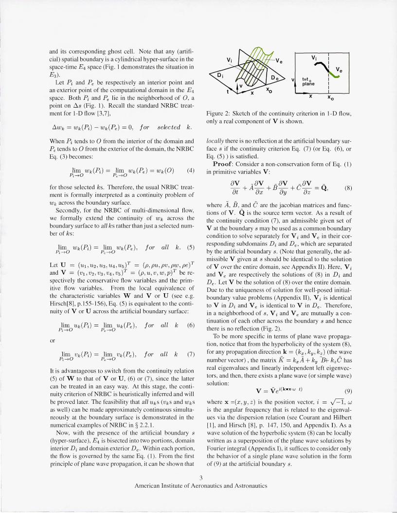
Figure 5 : Fl uxes ba lance on an internal face Si in E 3 .

boundary. Consider a triangular ce ll 6.ABC in E3 (FigA, shaded

area). Let P and Q, R , S be respectively the cell centers of 6.ABC and its ne ighboring triang ul ar cell s. Most o f the finite vo lume schemes use the space- time cy linder 6.ABC as the contro l vo lume (CV) for updating V or U a t P . Surface flux alo ng, say, AB is obtained by ex­trapolati on from S across the ce ll to the surface center along AB. Another treatment is to include S in the CV and replace the flux along AB by the fluxes along AS and S B. Since S s its right on both surfaces along AS and S B , no extrapo latio n across the interi or of the CV is invo lved. For the triangular cell 6. AB C in F ig. 4 the CV turns out to be a space- time hexagon cylinder in E3 based on ASBQCRA. By applying the integra l conser­vation laws (2) to the CV, updating fl ow data at P based on the fl ow data at a compact node stencil of Q, R, S is now completed. Fig. 4 also de mo nstrates that for quadrilateral mesh cells the CV is an octagon cy linder in E3 (2-D space).

The surface fluxes for the CV surfaces passing through a vertex , say, cell centers Q, R, S, can be evaluated by first extrapolating U alo ng the surface to their cor­res ponding surface centers by linear Tay lor ex pansio n, ca lc ul ating flu x funct ions Fo- and H , and then incor­porating the surface unit normal vector and computing the fluxes. For hi gh space dimensions, the CVs are geo­metrically more complicated. More details including the updating of U "" U y , and U z can be fou nd in [10,11 ].

It should be noted that the compact updating is sug­gested for boundary cell s only. For interior cell s , o ne may still continue to use other finite volume schemes.

2.3 Relation between an NRBC and the flux balance across the boundary surface

In thi s subsection , the re latio n between two sta teme nts is establi shed. The first one states that the incoming flu xes at the artific ia l bou ndary surface are equal to the o utgo­ing flu xes, or flu xes are balanced across the boundary

6

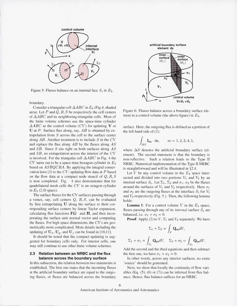
artificial boundary surface element ds

Figure 6: Fluxes ba lance across a boundary surface e le­me nt in a control vo lume (the above fi gure) in E 3 .

surface. Here , the outgo ing flux is defi ned as a porti o n of the left hand s ide of (2):

r 1m ' ds , l6s

m = 1, 2, 3,4, 5,

where 6.S denotes the artific ial boundary surface (el­eme nt). The second state me nt is that the boundary is no n-re fl ective . Such a re lati on leads to the Type II NRBC. Numeri ca l impleme ntat ion of the Type II NRBC is straightforward and wi ll be illus trated in §2A .

Let V be any control vo lume in the E4 space inte r­sected a nd divided into two portions VI and V2 by an internal surface Si . Let I\, ~2 and 0"1, 0"2 be the fluxes around the surfaces of VI and V2 respectively. Here 0"1

and 0"2 are the outgo ing flu xes at the interface Si for V1

and V2 respecti vely (Fig . 5 ). Then , the fo ll owing lemma ho lds:

Lemma 1: For a control volume V in the E4 space, flu xes pass ing through any of its internal surface Si are balanced , i.e. 0"1 + 0"2 = O.

Proof: Appl y (2) to V, VI and V2 separate ly. We have

~1 + ~2 = Iv QmdV,

~1 + 0"1 = r QmdV, l v) ~2 + 0"2 = r QmdV. l v.

Add the second and the third equations and then subtract the first one, we have 0"1 + 0"2 = O.

In other words, across any interior surfaces, no ex tra 'source' should be ge nerated .

Next, we show that locall y the continuity of fl ow vari­ables (Eq. (5), (6) or (7)) can be inferred from flu x bal ­ance. He nce, flu x balance suffices for an NRBC.

American Institute of Aeronautics and Astronautics

Consider an element ds of the cylindrical spati al boundary surface in E4 . As shown in the contro l vol­ume in Fig. 6 (in E 3 ), ds is centered at O. As­sume the outgoing unit normal vector at 0 is n1 = (nx , ny , n z , of, then, the incoming unit normal is n2 = (-nx , - ny , - n z, O)T. The outgo ing flu x 0"1 for the in­ner boundary surface:

a 1 = (

0"11 ) (Fl ) (Gl) (HI) ~2 ~ ~ ~ 0"13 = ds [n x F 3 +ny G3 +n z H 3 ]

~4 ~ ~ ~ 0"15 F5 G5 H 5

= ds [nxF + ny G + n zH ].

Let the outgoing boundary surface flu x vector be:

L = [nx F + ny G + n zH ],

then

L = O"l /ds.

Let V = (p,u ,v ,W,p)T be the primiti ve fl ow variable vector. L may be considered as a non-linear vector func­tion of V . The jacobian matrix g~ has the eigen values (e.g. see Hirsch [8], p. I77 ):

Al = A2 = A3 = u· nx + v . ny + W . n z ,

A4 = Al - C, A5 = Al + C.

where C is the speed of sound . If none of the eigenvalues vani shes at 0 , the jacobian g~ is non-singular, and an inverse vector function, the primitive fl ow variables V as a vector functi on of the surface flu x L ex ists. Thus,

Lemma 2: If the jacobian g~ is non-singul ar, then, loca ll y, the primitive variables V are uniquely de fined by the flu x vector L at the center 0 of ds.

Proof: Assume L (V 1) = L 1 and there is anothe r V 2 in the neighborhood of V 1, such that L (V 2) = L1. By a linear Tay lor expansion,

L (V 2) - L (V 1) =

8L 2 (8V )V=V1 (V 2 - V I) + 0 (I V 2 - V 11 ) = 0

Hence V 2 - V 1 = 0 or V 2 = V 1 since the first order term cannot cancel with the second order term.

From Lemma 2 and the NRBC continuity criteri on (7), it is inferred that locall y, under the condition that the ja­cobian g~ is non-singular, the foll owing lemma holds:

Lemma 3: For hyperbolic conservati on laws of gas dynamics, an element of the artificial boundary surface is non-refl ecti ve if its outgo ing flu xes and incoming flu xes are equal (balanced) .

7

boundary surface element 6s _______

control volume V

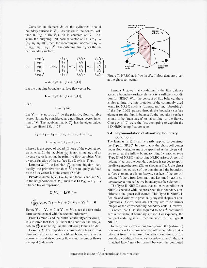
Figure 7: NRBC at inflow in E3 . Inflow data are given at the ghost cell center.

Lemma 3 states that conditionally the flux balance across a boundary surface element is a suffi cient condi­ti on for NRBC. With the concept of flu x balance, there is also an intuitive in terpretation of the commonl y used terms for NRBC such as ' transparent ' and 'absorbing'. If the flu x 10(% passes through the boundary surface element (or the flu x is balanced), the boundary surface is said to be ' transparent ' or 'absorbing' to the flu xes. Chang et al [9] were the fi rst attempting to explain the \-D NRBC using flu x concepts.

2.4 Implementation of absorbing boundary condition

The lemmas in §2.3 can be eas il y applied to construct the Type II NRBC. In case that at the ghost ce ll center nodes fl ow variables must be specified as the given val­ues (e.g. at the in fl ow boundary, Fig. 7), another type (Type II) of NRBC - absorbing NRBC ari ses. A control vo lume V across the boundary surface is needed to apply the di vergence theorem (2). As shown in Fig. 7, the ghost cell center lies outside of the domain , and the boundary surface element 6. s is an internal surface of the control vo lume V , then, from Lemma I and Lemma 3, 6. s is au­tomaticaLLya non-refl ective boundary surface element.

The Type II NRBC states that no extra condition of NRBC is needed with the prescribed fl ow boundary con­diti ons at the ghost cell center. This Type II NRBC is fl ex ible and valid with practicall y any cell shapes or con­fig urations. Ghost cell s are not required to be mirror images of the corresponding boundary cell s. However, it is noted that U is sti ll required to be C 1 continuous across the artifi cial boundary surface. Consequently, the compact updating is still recommended for the Type II NRBC.

In many cases, over a long time period, the (subsonic) fl ow may develop a fl ow near the infl ow boundary that is di fferent from the imposed boundary conditi ons, or the boundary condition becomes 'overdetermined', then, a 'matched layer' may be fo rmed between the computed

American Insti tute of Aeronautics and Astronautics

1 __ -

interi or fl ow and the imposed fl ow boundary condition (see Fig. 18). The situation is somewhat similar to that in the PML (perfectl y matched layer) method [5 ,6]. The shock-capturing numerical scheme should be able to quic kl y resolve thi s non-physica l di scontinuity in a few cell s .

2.5 Discussions on the NRBCs In practical applicati ons, due to di scretizati on, approxi­mation and lack of information in the domain exte rior, there are limitations for both Type I and Type II NRBCs.

For Type I NRBC, as mentioned in §2.2. 1, ex trapola­ti on technique might lead to drifting or dev iation from the true solution because no fl ow data outs ide the out­fl ow boundary is availab le. In addition, under the mirror image assumption on the ghost cell s in §2.2.1 and the as­sumption that the boundary surface 6.s is normal to the x ax is, the NRBC (12) implies that the NRBC continuity crite ri on (5 - 7) are sati sfied at any po int on 6.s . H ow­ever, as explained in the fo llowing, due to di scre ti zation and the poss ible consequent phase error, the accuracy of the NRBC could be degraded.

Consider a Fourier mode in the plane wave so lution (9): e i (k ex -w t ) . Here, B(x, t) = k • x - wt is the phase of the wave mode, wi th k being the wave number vec­tor in the propagation directi on. Generally, the directi on of k mayor may not be the same as the fl ow direction. O(x, t) = canst. s tands for a wavefront ( or a charac­teristic surface, see e.g. Hirsch [8], p.150, Courant and Hilbert [1] ). After di screti zation, the center 0 of 6.s (Fig. 3) is employed to represent the entire 6. s. Then how much phase error is introduced to the Fourier mode by the di screti zati on? Let x = (x , y , z) be the pos ition vec tor of any poin t on 6.s and Xo the pos ition vector of the center O. For clarity, assume time t is held un­changed . Then, after discretization , the phase erro r 6.B due to re placing x by Xo is :

6.B = k . x - k . Xo = k . (x - xo) (14)

note that 6.x = x - Xo lies on 6. s, 6.B = ° when k is normal to 6. s. Therefore, for Type I NRBC, the best result is obtained when the wave propagati on direction is normal or onl y s li ghtl y oblique to the boundary surface. Otherwise, a phase error of order O( 6.x) may be intro­duced. It deteri orates the accuracy of NRBC and causes numerical re fl ection.

For Type II NRBC, in add iti on to the s imil ar phase er­ror of Type I NRBC, there are other restric tions too. In §2.3 , Lemma 3 is conditionall y va lid because it is based on the o ne to one correspondence between the boundary surface flu x vector L and the primitive fl ow variab le vec­tor V . The latter relies on the non-sing ul ar ity of the jaco­bian gt- . In case that gt- is s ingul ar, Lemma 3 may fa il. In addition, Lemma 3 is val id onl y locall y. Globall y, the

8

x EXACT CE / SE ----------------- - -- - -----------

430.00 0. 000000 0000 0.000000000 0 431. 00 0 . 00 00000000 0 . 00 00 000000 4 3 2 . 0 0 0.000000 0000 0.0000000 000 433.00 0 . 0000000 001 0 . 0000000001 43 4 .00 0 . 00 00000014 0.0000000014 4 3 5 .00 0 . 00 00 000149 0. 0 0 0 000 014 9 436.00 0.000 0 0 01391 0 . 000000139 1 437.00 0 . 0 0 00 01112 5 0 . 00000 11125 438 . 00 0. 00 0 007 6294 0 . 0 0 000 7 6 294 43 9 .00 0 . 00 00448 5 27 0 . 00 0 0 4485 27 44 0.00 0 . 0002 26 043 6 0.00 0 2260 436 44 1. 00 0. 00 097 65 62 5 0. 0009 7 6 5625 44 2 . 00 0 .00 3 6166981 0 .00361 6 69 81 443.00 0.0114823007 0 . 01148 23 00 7 444. 00 0. 031250000 0 0 . 0312500000 445 . 00 0.072908065 0 0 . 0 7 2 90 80650 44 6 . 00 0. 145816129 9 0.1 4 581 61 299 447 .00 0.25 0 0000 0 00 0. 2 500000000 448.00 0.367 4 33623 1 0.367 4336231 449.00 0 .462 9 3735 61 0 . 4 62937356 1 45 0 . 00 0 .5 0 00 0 000 00 0. 50 0 0000000 4 51 .0 0 0 . 4 629373 561 0. 4 62937356 1

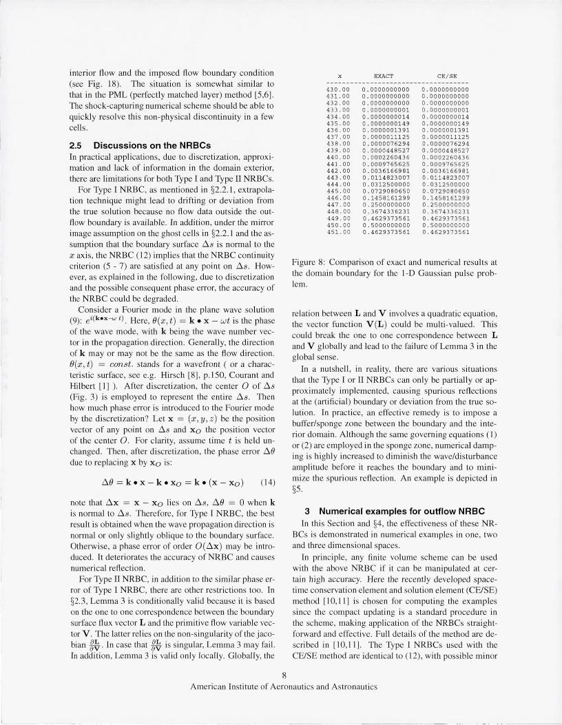
Figure 8: Comparison of exact and numerical results at the domain boundary for the 1-0 Gauss ian pu lse prob­lem.

re lat ion between L a nd V involves a quadratic equation, the vector function V eL) could be mu lti-valued. This could break the one to one correspondence between L and V g loball y and lead to the fai lure of Lemma 3 in the global sense.

In a nutshell, in reality, there are various s ituations that the Type l or II NRBCs can only be parti ally or ap­prox imately implemented, causing spurious re fl ections at the (artifi c ial ) boundary or dev iati on from the true so­lution. In practice, an effective remedy is to impose a buffer/sponge zone between the boundary and the inte­rior domain . Although the same governing equati ons (1) or (2) are employed in the sponge zone, numerical damp­ing is highl y increased to dimini sh the wave/disturbance amplitude before it reaches the boundary and to mini ­mi ze the spuri ous refl ectio n. An example is depicted in §5.

3 Numerical examples for outflow NRBC In thi s Section and §4, the effectiveness of these NR­

BCs is demonstrated in numerica l examples in one, two and three dime ns iona l spaces.

In principle, any fi nite vo lume scheme can be used with the above NRBC if it can be manipulated at cer­tain high accuracy. Here the recentl y developed space­time conservati on element and solution e lement (CE/SE) method [10,11] is chosen for computing the examples since the compact updating is a standard procedure in the scheme, making application of the NRBCs s tra ight­forward and effective. Fu ll details of the method are de­scribed in [10,11]. The Type I NRBCs used with the CE/SE method are identical to (12) , with poss ible minor

American Institute of Aeronautics and Astronautics

l.

l"ITf l n ..,lIi1l11 a oc1 1450"" il

0.6 Cat. problem 1.1, cfl=1,ep=O, 1=450

0.5 ---- numerical

0.4 L ••••••• • ••• exact

0.3

U 0.2

0.1

o.o E ---

430 435 440 X 445

0.6

0.0

450

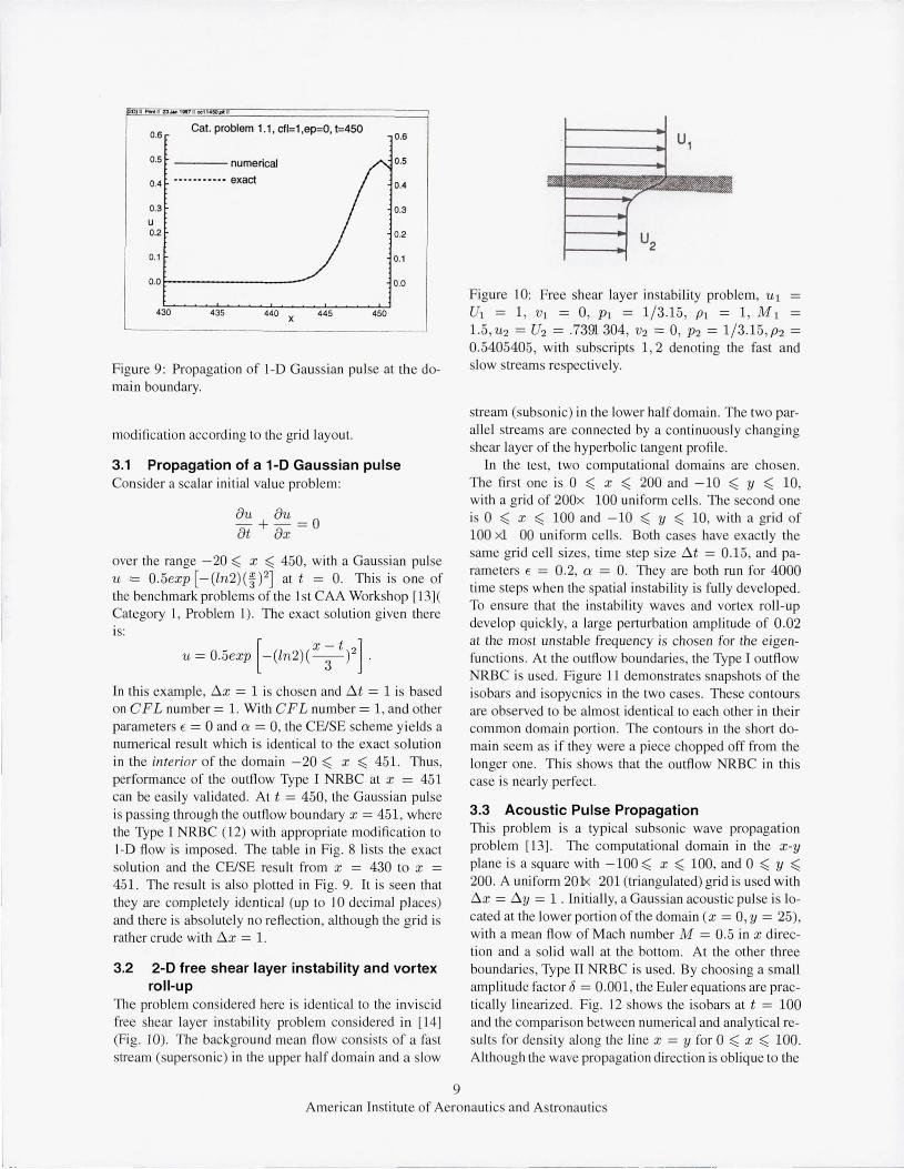
F igure 9: Propagati on of l-D Gauss ian pulse at the do­main boundary.

modification according to the grid layout.

3.1 Propagation of a 1-0 Gaussian pulse Consider a scal ar initi al va lue problem:

au au_ o at + ox -over the range - 20 ~ x ~ 450, with a Gaussian pulse u = 0.5exp [- ( ln2)(~)2] at t = O. This is o ne o f the benchmark problems of the 1st CAA Workshop [1 3]( Category I , Problem I ). The exact so lution given there is:

[X - t ] u = 0.5exp -(ln2)(-3-? .

In thi s example, ~x = 1 is chosen and ~t = 1 is based on CFL number = 1. With CFL number = 1, and other paramete rs E = 0 and a = 0, the CE/SE scheme y ie lds a numerical result which is identical to the exact so lutio n in the interior of the do main -20 ~ x ~ 451. Thus, performa nce of the outfl ow Type I NRBC at x = 451 can be easily va lidated. At t = 450, the Gauss ian pulse is pass ing throug h the outfl ow boundary x = 451, where the Type I NRBC (1 2) with appropri ate modificati on to ] ·D fl ow is imposed . The table in Fig . 8 lists the exact solution and the CE/SE result fro m x = 430 to x = 451. The result is a lso plotted in Fig. 9. It is seen that they are completely identi cal (up to 10 decimal places) and there is abso lutely no re fl ecti on, although the grid is rather crude with ~x = 1.

3.2 2-D free shear layer instability and vortex roll -up

The problem considered here is identical to the invisc id free shear layer instabili ty proble m considered in [1 4] (Fig. 10). The background mean fl ow consists of a fas t stream (supersonic) in the upper half domain and a slow

9

U1

U2

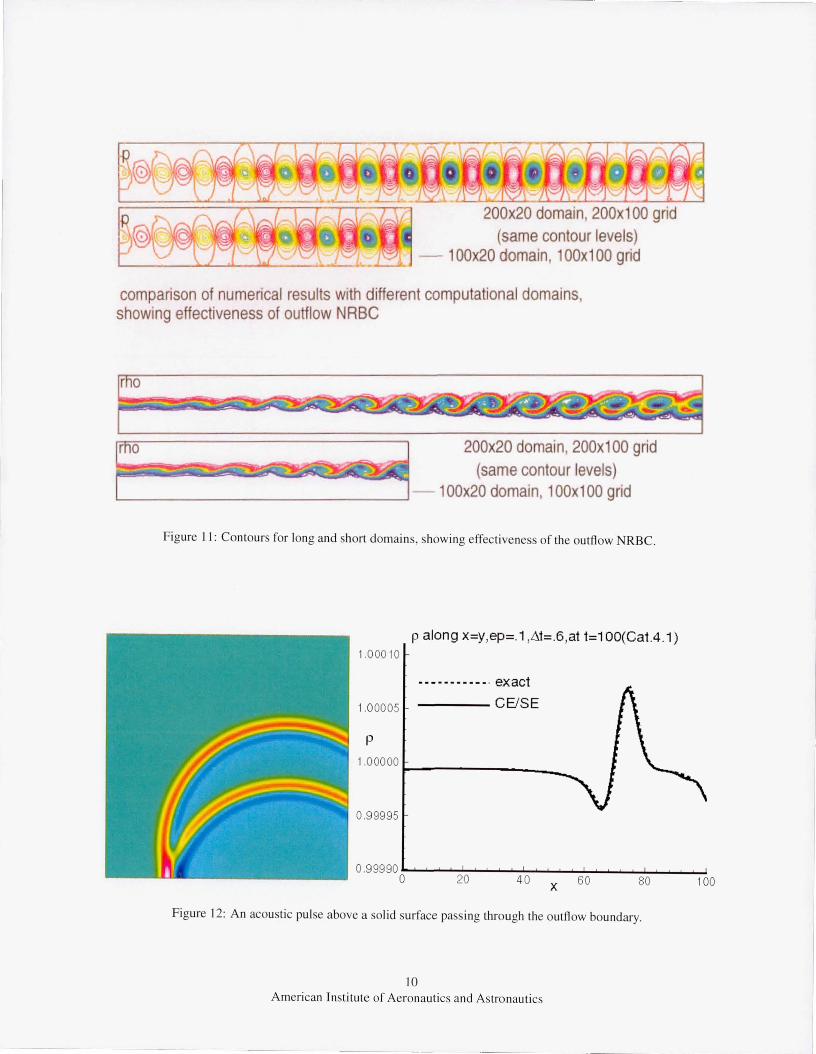
Figure 10: Free shear layer instabili ty problem, Ul = U1 = I , Vi = 0, Pi = 1/ 3.15, Pi = I , M 1 = 1.5,U2 = U2 = .7391304, V2 = 0, P2 = 1/3. 15, P2 = 0.5405405, with subscripts 1, 2 denoting the fas t a nd s low streams respecti vely.

stream (subsonic) in the lower half doma in . The two par­a ll e l streams are connected by a continuously chang ing shear layer of the hype rbolic ta ngent pro fi le.

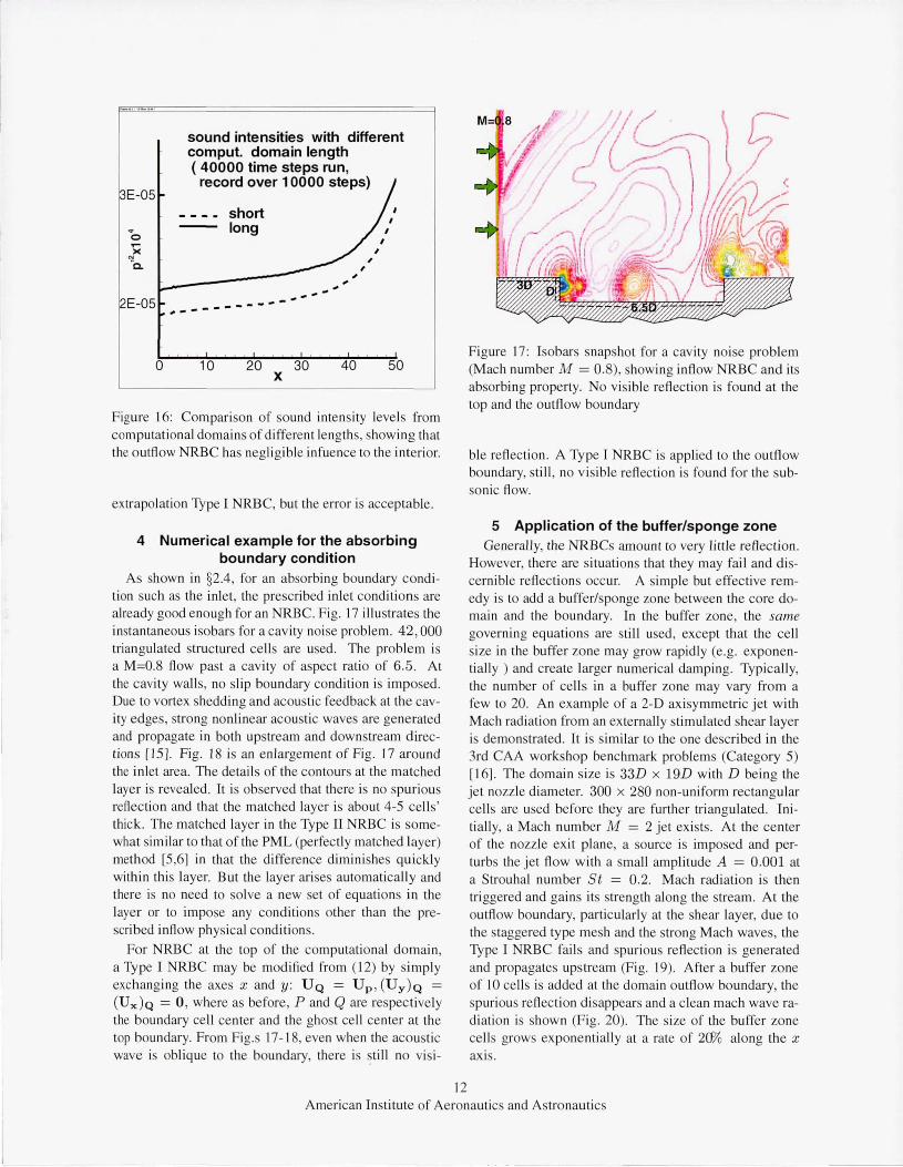
In the test, two computati onal domains are chosen. The first one is 0 ~ x ~ 200 and -10 ~ Y ~ 10, with a grid of 200x 100 uniform cell s. T he second o ne is 0 ~ x ~ 100 and - 10 ~ Y ~ 10, with a grid of 100 xl 00 unifo rm cells. Both cases have exactl y the same grid cell sizes, time step size ~t = 0.15, and pa­rameters E = 0.2, a = O. They are both run for 4000 time steps whe n the spa ti a l instability is full y developed. To ensure that the instabi lity waves and vortex roll-up develop qui ckl y, a large perturbation amplitude of 0.02 at the mos t uns table frequency is chosen for the eigen­functi ons. At the outfl ow boundaries, the Type I outfl ow NRBC is used . Fig ure I I de monstrates snapshots of the isobars and isopycnics in the two cases. These conto urs are observed to be a lmost identical to each other in their common doma in porti o n. The contours in the short do­main seem as if they were a piece chopped off from the longer one. This shows that the outflow NRBC in thi s case is nearl y perfect.

3.3 Acoustic Pulse Propagation This problem is a typical subsonic wave propagation problem [1 3]. The computational domain in the x -y plane is a square with - 100 ~ x ~ 100, and 0 ~ y ~ 200 . A uni fo rm 20lx 201 (triangulated) grid is used with ~x = ~y = 1 . Initi ally, a Gaussian acoustic pulse is lo­cated at the lower porti o n of the domain (x = 0 , y = 25), with a mean fl ow of M ach number M = 0. 5 in x direc­ti on and a solid wa ll a t the bottom. At the other three boundari es, Type II NRBC is used. By choosing a small amplitude facto r b = 0.001, the Euler equations are prac­tica ll y lineari zed. Fig. 12 shows the isobars at t = 100 and the compari son between numerical and analyti ca l re­sults for density along the line x = y for 0 ~ x ~ 100. Althoug h the wave pro pagati on directi on is oblique to the

A meri can Institute of Aeronautics a nd Astronauti cs

----------------------------_._._ .. _. __ .. _ ..

200x20 domam, 200x100 grid (same contour levels)

' . J , I ' cI - , ). s' .J.,--~J - 1 00x20 domain, 1 00x1 00 grid

comparison of numerical results with different computational domains, showing effectiveness of outflow NRBC

200x20 domain, 200x100 grid (same contour levels)

1...--.. ____________ -.l,- 100x20 domain, 100x100 grid

Figure II : Contours for long and short domains, showi ng effecti veness of the outfl ow NRBC.

p along x=y,ep=.1 ,L1t= .6,at t=1 00(Cat.4 .1) 1.000 10

- - - - - - - - - - - , ex act

1.0 0005 ----CEISE

P

1.0 00 00 l-f-------_

0.99995

!! t ! ! [ , t ! , !

.. , 0.99990 t 20 40 x 60 80 '---------

Figure 12: An acoustic pulse above a solid surface pass ing through the outfl ow boundary.

10 American Institute of Aeronautics and Astronautics

100

~1-........ Computational ~;' : ........ ..... Domain

/~ ............ , ........ ........ /

,. I -r ..... ", '" I ..... .... ....

~,. '" I rec tangular .............

\

j......... I no zzle .... ........ I .... .... J ........ ;:::.

I "."... .......... ,,"" I I ".:<............. '" I

H I r:::;. '" ..... .... .... ..... ..... ..... ..... ",, '" I I '" .... .... .... '" I

II ."."" n o zzle ............. .... ...... .... ,,/' I I ",,'" lip wall .... .....;:<.. I I ", ........ "'..... I <. .... r .... .... I

~.... ........ : ........ ........ ) ~.... .... I '"

L ............. ........ : / ", / /

rectangular ~'....... .... I ",/ no z zle inner ~........ I, ........ ........ .... narro w side = D, wide side - 50 .

........ ...!..".'"

F igure 13: Sketch of the rectangular jet, aspect ra tio 5, jet Mach number MF 1 .6 , L = 16D, W = 16D and H = 5.6D.

outflow boundary, only tiny re fl ecti o n is observed from Fig. 12. Another 2-D example with complete ly subsonic fl ow will be illustrated in §4.

3.4 3-~ rectangular jet flow Fig. 13 is the sketch of an underexpanded rectangular jet in 3-D space. The rectangular nozzle protrudes into the compu tati onal domain by l = 2D , D be ing the width of the jet. The unstructured mesh consis ts of about 1. 7 mil ­lion tetrahedral cell s. At the in let plane, ambient (s ta tion­ary) condition is specified. Jet fl ow at higher press ure is spec ified at the nozzle ex it. All the rest boundaries are e i­ther Type I or Type II NRBC. Fig.s 14 shows snapshots o f the isobars and v veloc ity contours on the cross secti onal mid-planes after running 60,000 time steps. Fig. 15 demonstrates the 3-D pressure iso-surfaces. No visible refl ecti on is observed.

3.5 Influence of the NRBC to the numerical accuracy

When the outflow boundary is non-refl ecting, the influ­ence from the boundary to the interi or fl ow is small . Fig. 16 demonstrates the sound intensity leve l computed based on two domains with different lengths but same width for the 2-D Mach radiation problem in the 3rd CAA Workshop (Category 5) [1 6]. The short domain has a grid of 2ffi x 144 nodes. The onl y di fference is that the longer domain has 30 more uni form ly di stribu ted nodes added in the x directi on downstream. Fig. 16 shows the sound intensity levels (square of r.m.S. p' - pressure flu c­tuation ) along the line y = 10 at t = 400 (40000 time steps or 28 periods) for bo th domains. It is observed that the max imum diffe rence is about 2 x 10- 10 , fa r be­low the di screti zati on error, thus is negli gible. Thi s case also demonstrates the relati ve dri ft ing side effect of the

II

I~ It.~ . '-

v- contours on the mid plane (narrow side)

v-contours on the mid- plane (wide side)

Figure 14: v veloc ity contours on the mid-planes w ith mesh bac kground. No visib le re fl ection is observed. At the outflow boundary, fl ow is supersonic in the jet core and then becomes subsonic across the thi ck shear layer.

p isosurfaces from the narrow side

vortical structure

p isosurfaces from the wide side

NRBC

Figure 15: Pressure iso-surfaces, no refl ection is ob­served .

Ameri can Institute of Aeronautics and Astronauti cs _J

E-05

.. o ~

>< N -0.

E-05

o

sound intensities with different com put. domain length ( 40000 time steps run,

record over 10000 steps)

short long

~ .. -.. -----;;-.

10 20 30 x

40 50

F igure 16: Comparison of sound inte nsity levels from computational domains of di ffe rent lengths, showing th at the outflow NRBC has neglig ible infuence to the inte ri or.

ex trapolation Type I NRBC, but the error is acceptable.

4 Numerical example for the absorbing boundary condition

As shown in §2.4, for an absorbing boundary condi ­tion such as the inlet, the prescribed inlet conditions are already good enough for an NRBC. Fig. 17 illustrates the instantaneous isobars for a cavity noise problem. 42 , 000 tri angulated structured cells are used. The proble m is a M=0.8 fl ow past a cavity of aspect ra tio o f 6 .5. At the cavity wall s, no slip boundary condition is imposed. Due to vortex shedding and acoustic feedback at the cav­ity edges, strong nonlinear acousti c waves are gene rated and propagate in both upstream a nd downstream direc­tions [15J. Fig. 18 is an enl argement of Fig. J 7 aro und the inlet area. The detail s of the contours at the matched layer is revealed. It is observed that there is no spurious refl ecti on and that the matched layer is about 4-5 cell s ' thick. The matched layer in the Type II NRBC is some­what similar to that of the PML (perfectl y matched layer) method [5 ,6J in that the difference dimini shes quick ly within this laye r. But the layer ari ses automati cally and there is no need to solve a new set of equations in the layer or to impose any conditions other than the pre­scribed inflow phys ical conditions.

For NRBC at the top of the computational domain , a Ty pe I NRBC may be modified from (1 2) by s impl y exchang ing the axes x and y : U Q = Up , (Uy )Q = (Ux )Q = 0 , where as be fore, P and Q are respecti vely the boundary ce ll center and the ghost cell center at the top boundary. From Fig.s 17- 18, even when the acousti c wave is oblique to the boundary, there is still no vis i-

12

"/ , ,-

" f , / { , '-/ (o' __ ., . ,,-

. . "~-, ~ ..... , ;t ,

'.

Figure 17: Isobars snapshot for a cav ity no ise problem (Mach number M = 0.8), showing inflow NRBC and its absorbing property. No vis ible refl ection is found at the top and the outfl ow boundary

ble re fl ecti on. A Ty pe I NRBC is applied to the outflow boundary, still , no v isible re fl ecti on is found fo r the sub­so nic fl ow.

5 Application of the buffer/sponge zone Ge nerally, the NRBCs amount to very little refl ec ti on.

However, there are s ituati ons th at they may fa il and di s­cernible re fl ecti ons occur. A simple but effecti ve rem­edy is to add a buffe r/sponge zo ne between the core do­ma in and the boundary. In the buffer zone, the same governing equations are still used, except that the cell s ize in the buffe r zone may grow rapidly (e.g. expone n­ti a lly ) and create larger numerical damping. Typicall y, the number of cell s in a buffer zo ne may vary fro m a few to 20. An example of a 2-D ax isymmetri c je t with Mach radi ati on from an externall y stimulated shear layer is demonstrated . It is similar to the one described in the 3rd CAA workshop benchmark pro blems (Category 5) [16J. The domain s ize is 33D x 19D with D be ing the jet nozzle di ameter. 300 x 280 non-uniform rectangular cell s are used before they are further triangulated . Ini ­ti a ll y, a Mach number M = 2 jet ex ists. At the ce nter of the nozzle exit plane, a source is imposed and per­turbs the jet fl ow with a small ampli tude A = 0 .001 at a Strouhal number St = 0. 2. Mach radi ati on is then tri ggered and gains its strength along the stream. At the outflow boundary, parti cularl y at the shear layer, due to the staggered type mesh and the strong Mach waves, the Type I NRBC fail s and spurious re fl ecti on is genera ted and propagates upstream (Fig. 19). After a buffer zo ne of 10 cell s is added at the domain outflow boundary, the spurious refl ecti on di sappears and a clean mach wave ra­di ati on is shown (Fig. 20). The s ize of the buffer zone cell s grows expone nti all y at a rate of 2(% along the x ax is.

A merican Institute of Aeronautics and Astro nauti cs

Figure J 8 : Deta il s of the contours at the inflow boundary, showing the matched layer at the inlet and its spreading over the grid.

F igure 19: Mach radi ation from a M = 2 axisymmetric jet (without buffer zone), showing severe spurious nu­meri ca l re fl ecti on.

13

p

Figure 20: Mach radi ation from a M = 2 ax isymmetri c jet (with buffe r zone but not shown), showing a c lean acoustic field .

6 Concluding Remarks In the present paper, the hyperbolicity of the E uler

equati on system and the propagati on of plane waves are rev isited, and then combined to deri ve the continuity criteri on of NRBC. The rela ti on between flu x balance across the boundary surface and the NRBC is estab­li shed. Simple but effecti ve C 1 continui ty NRBCs are consequentl y developed.

These NRBCs are simple a nd robust, as demonstrated in the one and mul ti-dimens ional numeri cal examples based on the the recent CE/SE method. Numerical examples with other finite volume schemes, e.g., N.T. (Nessyahu and Tadmor) or upwind schemes can be fo und in [17] (§8). Generall y, the ir perfo rmances are similar to those of the characteri stics-based NRBCs. Limitations of the NRBCs are also di scussed in §2.5 . In particul ar, the Type I extrapolation NRBCs may cause solution drifting due to lack of informati on beyond the (outfl ow) bound­ary. A remedy is to incorporate the phys ical boundary conditions or to use a sponge zone.

The di versity of various NRBCs in fl ow computations can never be overestimated. The purpose of the present pape r is to show some guide lines in thi s direction a nd develop NRBCs th at are simple but robust for practica l computati ons. The compact updating procedure proves to work well with the NRBCs and prov ides C 1 acc u­racy in surface flu x eva luati on. But it is de finitely not the only way to achieve non-refl ecting effect. Different schemes may have different treatments. Sometimes , a combinati on of the NRBC treatments may prov ide much improved results, such as the incorporati on of the buffer zone. As a byproduct, we are now able to explain wh y the NRBCs with the recentl y developed CE/SE scheme [ 10,11 ,14,15] are robust.

The restric ti on in §2. l that the fl ow is continuous may be li fted, since fo r shock-capturing schemes, a discon-

A merican Institute of Aeronautics and Astronautics

tinuity may be considered as a continuous wave with steeper gradient. But if the wave propagation direction is ob lique to the (artifi c ial ) boundary, the NRBC may per­form poorly due to reasons expla ined in §2.5. Chang et at [9] , Huynh [17] presented 1-D examples ( i.e. wave propagati on directi o n no rmal to the boundary) showing how a shock passes through an arti fi c ial boundary with­out causing visible re fl ec ti on.

At last, we comment on the influence of the errors of the NRBCs on the accuracy for domain inte ri or. G ener­a ll y speaking, thi s involves the stability property of the sche me. If the time-marching explicit scheme sati sfi es the von Neumann stabi lity crite ri o n, an error introduced by the boundary conditi o n wi ll decay exponentia ll y in time and space when it convects towards the domain in­teri o r.

Acknowledgements This work received support from the Supersoni c

Propuls ion Technology Projec t Office of NASA G lenn Researc h Cente r. The author wishes to thank Drs. R.Hixon, R. Bl ech, P.C.E . Jorgenson, A. Himansu and x.Y. Wa ng for fruitfu l di scussions on the issues in the present paper.

References [I] Courant, R. and Hi lbert,D. " M ethods of Mathe mat­

ical Physics", VoI.II, John Wiley & Sons, London, 1962.

[2] Givoli ,D. , "No n-refl ecting Boundary Conditi o ns", 1. Comput. Phys. , Vo l. 94 , 1-29(199 1).

[3] Engquist, B . and M ajda, A. , "Absorbing boundary conditi ons for the numerical simulati o n of waves", Math . Camp. , Vol. 31 , pp. 629-65 1 (1977).

[4] Tho mpson, K. W "Ti me-dependent boundary con­ditio ns for hyperbolic systems" , i & ii , 1. Comput. Phys. , Vo l. 68, pp. 1-24, (1987); a lso Vol 89, pp 439-461 , (1 990).

[5] Hu , F.Q. , "On Absorbing Boundary Conditions for Lineari zed Eul er Equati ons by a Perfectl y Matched Layer" ,J. Com put. Phys ., Vo1.l29, 20 1-2 19 (1996).

[6] Hesthaven, lS .,"The Analys is and Co nstructi on of Perfectly Matched Layers fo r the Lineari zed E ul er Equations", ICASE Report No. 97-49 ( 1997) (a lso in I . Compu£. Phys.)

[7] Hedstrom,G .W , " Nonrefl ecting Boundary Condi­ti ons fo r Nonlinear Hyperboli c Systems" , 1. Com­put. Phys. , Vo 1.30, 222-237 (1979) .

[8] Hirsch, C. "Numerical Computation ofIntern a l and Ex ternal Flows" , Vo l. II, John Wiley & Sons ( 1993).

14

[9] Chang, S. c. , Himansu, A. , Loh, C. Y., Wang, X. Y. , Yu, S.-T. and Jorgenson, P. C. E . "Robust and Sim­ple Non-Re fl ecting Boundary Conditions for the Space-Time Conservati on E lement and So luti o n E l­ement Method ", AIAA Paper 97-2077 ( 1997).

[10] Chang, S. c. , Wa ng, X . Y. and Chow, C. Y. , " The Space-Time Conservation E leme nt and Solutio n E l­ement Method - A New High-Resolu tion and Gen­uine Mu ltidimensio na l Paradig m for Sol ving Co n­servation Laws ", 1. Comput. Phys. vo l. 156, pp. 89- 136 ( 1999).

[11] Wang, X .-Y. and Chang S.-c. , " A 2-D N o n­spli tting U nstructured Triang ul ar Mesh E uler Sol ver Based o n the Space-Ti me Co nservati o n E l­e ment and S olution E lement Method" CFD 1. vol. 8, pp309-325 ( 1999).

[1 2] Nessyahu , H . a nd Tadmor, E . "Non-oscill a tory Ce ntra l Di ffewre nc ing fo r Hyperbolic Conservati on Laws", 1. Comput. Phys. , Vo1. 87 , 408-463 ( 1990) .

[ 13] "ICASElLaRC Workshop o n Benchmark Proble ms in Computational Aeroacoustics", Eds. lHardin , J.R.Ri storcelli , and C.K.WTam, NASNCP-3300 ( 1994).

[ 14] Loh , C. Y. , Hultgren, L. S. and Chang S.-c. , "Computing Waves in Compressible F low Using the Space-Time Conservatio n E lement Solu tion E l­ement Method," AlAA 1., Vol. 39, pp. 794-80 I (2001 ).

[15] Loh, Ching Y. , Wang, Xiao Y. , Chang, Sin-Chung and Jorgenson, Philip c.E. , "Computati on of Feed­back Aeroacousti c System by the CE/SE M ethod", in proceedings of the 1st Int ' l Conf. on CFD (IC­CFD), Kyoto, Japan, Jul y, 2000; (publis hed by Springer-Verlag, 2001 ).

[16] "Third Computational Aeroacousli cs Workshop o n Benchmark Problems" , NASNCP-2000-209790.

[17] Huynh , H.T. , "Compari son and Improvement of Upwind and Centered Schemes on Quadrilateral and Triangular M eshes", AIAA Paper 2003-3541 (2003).

Appendix I: Plane wave solutions The plane wave so lutions are based o n the Cauchy's

method of Fourier Integral (see Courant and Hilbert[l], pp.2 10-2 11 ) for li near homogeneous differenti a l equa­ti on. Consider Eq . (8):

aV -aV -aV -aV -7ft +A ax + B a:;; +C-y; = Q,

American Institute of Aeronautics and Astronautics

~ F igure 2 1: Continuity criterion in I-D fl ow.

In the neighborhood of a point 0 (xo , to) at the artifi ­cial boundary, (8) can be loca ll y linearized by setting the jacobians A, E, C to their va lues at O. Assume a plane wave with the fo rm V = Y eiO , and substitute in (8) . Here () = () (x , t) = x. k - wt is the phase of the simple wave, i = J=T. () = canst . stands for a characteristic surface or wave fro nt [J ]. (8) then becomes:

aY -aY - aY - aY - - - ·0 (-+A-+B -+C-)+i( K-wI )V = Q e- t

, at ax ay az where I is the 5 Xl identity matri x. For any given wave number vector k = (kx , ky, kz ), fro m the hyperboJicity of (8), rea l ~s exist such that k - wI = 0 (di spersion relation), where the matrix k = kxA + ky E + kzC. Then the 'amplitude' Y may be solved fro m

aY -aY - aY - aY - - iO -+A-+ B -+C-= Qe at ax ay a z

For more general waves other than the simple plane waves, as (8) is locally lineari zed in the neighborhood of the boundary point O(xo , to), they may be decomposed by Fourier integral with respect to wave number k and repl aced by the superpos ition of plane waves.

Appendix II: Discussions on the continuity criterion and the extrapolation technique

Without loss of generali ty, consider a I-D fl ow shown in F ig. 2 1. As a pure ini ti al value Cauchy problem, V = V (x, O) at t = 0 is given. This problem is well ­posed and there exists a unique soluiton V = V o(x, t) over the entire domain D : -00 < x < 00, t ~ O. If a boundary exists on the left inlet side, the pro blem becomes an initial-boundary-value problem, a boundary condition is required at the inlet boundary.

Assume the art ific ial boundary locates at x = 0 and bisects the entire domain D into domain interior Di and domain ex terior De: D = Di + De (see §2. 1). In order that V i and V e in §2. 1 are respecti vely the unique well ­posed solutions in subdomains Di and De, an admi ssible common boundary cond ition they share at x = 0 is:

V ieO, t) = V e(O, t) = V o(O, t).

Here, V o(O, t) is the entire domain solution along the line x = 0; or equivalently, V o(O, t) may be obta ined

15

--- --- -- --,

by the method of characteristics as sketched in Fig. 2 1 at point 0 at the boundary.

However, fo r NRBC problems in reality, V o(x, t) , x ~ 0; or V e(x , t) is totally miss ing (otherwise there is no need to investigate the NRBCs). In this situation, the extrapolation technique e.g. (12) is not an unreasonable choice fo r the NRBC co ntinuity criterion. The ini ti al-boundary va lue problem fo r V i is well -posed onl y when the fl ow is supersonic or is kn own to remain unchanged across the artifi cial boundary at x = 0 by a priori info rmati on. Otherwise, even though locally the extrapolati on (12) leads to non-refl ecting effect, globally the 'so lution' will keep dri ft ing away and deviate fro m the true solution. The fo llowing are some remedies fo r practica l numerica l fl ow computations:

[ I ] use a sponge (bu ffer) zone with highly increased nu­merical damping to fi lter away the wave ingredients in the fl ow; when the Type I ex trapolati on NRBC is app lied to the outer outfl ow boundary, the fl ow is already uniform at the boundary.

[2] incorporate the extrapolation with other phys ical boundary conditions (e.g. back pressure etc.).

Notice that the present discussions do not apply to the Type II NRBCs.

American Institute of Aeronautics and Astronautics