Embed Size (px)
Citation preview
Beamforming of Ultrasound Signals from 1-D and2-D Arrays under Challenging Imaging Conditions
by
Marko Jakovljevic
Department of Biomedical EngineeringDuke University
Date:Approved:
Gregg Trahey, Supervisor
Stephen Smith
Jeremy Dahl
Jeffrey Krolik
Rendon Nelson
Dissertation submitted in partial fulfillment of the requirements for the degree ofDoctor of Philosophy in the Department of Biomedical Engineering
in the Graduate School of Duke University2015

ABSTRACT
Beamforming of Ultrasound Signals from 1-D and 2-DArrays under Challenging Imaging Conditions
by
Marko Jakovljevic
Department of Biomedical EngineeringDuke University
Date:Approved:
Gregg Trahey, Supervisor
Stephen Smith
Jeremy Dahl
Jeffrey Krolik
Rendon Nelson
An abstract of a dissertation submitted in partial fulfillment of the requirements forthe degree of Doctor of Philosophy in the Department of Biomedical Engineering
in the Graduate School of Duke University2015

Copyright c© 2015 by Marko JakovljevicAll rights reserved except the rights granted by the
Creative Commons Attribution-Noncommercial Licence

Abstract
Beamforming of ultrasound signals in the presence of clutter, or partial aperture block-
age by an acoustic obstacle can lead to reduced visibility of the structures of interest and
diminished diagnostic value of the resulting image. We propose new beamforming meth-
ods to recover the quality of ultrasound images under such challenging conditions. Of
special interest are the signals from large apertures, which are more susceptible to par-
tial blockage, and from commercial matrix arrays that suffer from low sensitivity due to
inherent design/hardware limitations. A coherence-based beamforming method designed
for suppressing the in vivo clutter, namely Short-lag Spatial Coherence (SLSC) Imaging,
is first implemented on a 1-D array to enhance visualization of liver vasculature in 17
human subjects. The SLSC images show statistically significant improvements in ves-
sel contrast and contrast-to-noise ratio over the matched B-mode images. The concept
of SLSC imaging is then extended to matrix arrays, and the first in vivo demonstration
of volumetric SLSC imaging on a clinical ultrasound system is presented. The effective
suppression of clutter via volumetric SLSC imaging indicates it could potentially com-
pensate for the low sensitivity associated with most commercial matrix arrays. The rest of
the dissertation assesses image degradation due to elements blocked by ribs in a transtho-
racic scan. A method to detect the blocked elements is demonstrated using simulated, ex
vivo, and in vivo data from the fully-sampled 2-D apertures. The results show that turn-
ing off the blocked elements both reduces the near-field clutter and improves visibility of
anechoic/hypoechoic targets. Most importantly, the ex vivo data from large synthetic aper-
iv

tures indicates that the adaptive weighing of the non-blocked elements can recover the loss
of focus quality due to periodic rib structure, allowing large apertures to realize their full
resolution potential in transthoracic ultrasound.
v

To friends and family for always believing in me.
vi

Contents
Abstract iv
List of Tables xi
List of Figures xii
Acknowledgements xvi
1 Background and Introduction 1
1.1 Overview . . . . . . . . . . . . . . . . . . . . . . . . . . . . . . . . . . 1
1.2 Clinical Motivation . . . . . . . . . . . . . . . . . . . . . . . . . . . . . 2
1.2.1 Problem of Image Clutter . . . . . . . . . . . . . . . . . . . . . . 4
1.2.2 Problem of Blocked Elements . . . . . . . . . . . . . . . . . . . 5
1.3 Conventional Ultrasound Imaging . . . . . . . . . . . . . . . . . . . . . 6
1.3.1 Delay and Sum Beamforming . . . . . . . . . . . . . . . . . . . 7
1.3.2 Speckle Statistics . . . . . . . . . . . . . . . . . . . . . . . . . . 9
1.3.3 Covariance of the Received Pressure Field . . . . . . . . . . . . . 13
1.4 Beamforming Limitations and Image Degradation . . . . . . . . . . . . . 14
1.4.1 Effects of Phase Aberration . . . . . . . . . . . . . . . . . . . . 14
1.4.2 Reverberation Clutter . . . . . . . . . . . . . . . . . . . . . . . . 16
1.4.3 Limited Acoustic Window . . . . . . . . . . . . . . . . . . . . . 17
1.4.4 Image Degradation due to Blocked Elements . . . . . . . . . . . 18
1.5 Adaptive Imaging Methods . . . . . . . . . . . . . . . . . . . . . . . . . 19
vii

1.5.1 Phase Aberration Correction . . . . . . . . . . . . . . . . . . . . 20
1.5.2 Clutter Suppression via Coherence-based Imaging Methods . . . 22
1.5.3 Compensation for the Blocked and Missing Elements . . . . . . . 24
1.6 Imaging with Matrix Arrays . . . . . . . . . . . . . . . . . . . . . . . . 26
2 Short-Lag Spatial Coherence Imaging on 1-D Arrays: Results of a Pilot Studyon Human Livers 31
2.1 Introduction . . . . . . . . . . . . . . . . . . . . . . . . . . . . . . . . . 31
2.2 Methods . . . . . . . . . . . . . . . . . . . . . . . . . . . . . . . . . . . 34
2.2.1 Short-Lag Spatial Coherence Imaging . . . . . . . . . . . . . . . 34
2.2.2 Clinical study . . . . . . . . . . . . . . . . . . . . . . . . . . . . 35
2.2.3 Data Processing and Statistical Analysis . . . . . . . . . . . . . . 36
2.3 Results . . . . . . . . . . . . . . . . . . . . . . . . . . . . . . . . . . . . 38
2.4 Discussion . . . . . . . . . . . . . . . . . . . . . . . . . . . . . . . . . . 44
2.5 Conclusion . . . . . . . . . . . . . . . . . . . . . . . . . . . . . . . . . 46
3 Short-lag Spatial Coherence Imaging on Matrix Arrays: Phantom and In VivoValidation 48
3.1 Introduction . . . . . . . . . . . . . . . . . . . . . . . . . . . . . . . . . 48
3.2 Methods . . . . . . . . . . . . . . . . . . . . . . . . . . . . . . . . . . . 50
3.2.1 Short-Lag Spatial Coherence Imaging on Matrix Arrays . . . . . 50
3.2.2 Rapid Single Channel Acquisition . . . . . . . . . . . . . . . . . 51
3.2.3 Flow Phantom Experiment . . . . . . . . . . . . . . . . . . . . . 52
3.2.4 In Vivo Experiments . . . . . . . . . . . . . . . . . . . . . . . . 53
3.2.5 Data processing . . . . . . . . . . . . . . . . . . . . . . . . . . . 53
3.3 Results . . . . . . . . . . . . . . . . . . . . . . . . . . . . . . . . . . . . 54
3.4 Discussion . . . . . . . . . . . . . . . . . . . . . . . . . . . . . . . . . . 60
3.5 Conclusion . . . . . . . . . . . . . . . . . . . . . . . . . . . . . . . . . 64
viii
4 Blocked Elements Signal Characteristics and Impact on Visualizing Anechoicand Hypoechoic Targets 66
4.1 Introduction . . . . . . . . . . . . . . . . . . . . . . . . . . . . . . . . . 66
4.2 Methods . . . . . . . . . . . . . . . . . . . . . . . . . . . . . . . . . . . 69
4.2.1 Full-wave Simulations . . . . . . . . . . . . . . . . . . . . . . . 69
4.2.2 Phantom Experiments . . . . . . . . . . . . . . . . . . . . . . . 71
4.2.3 In Vivo Study . . . . . . . . . . . . . . . . . . . . . . . . . . . . 72
4.2.4 Data Processing and Receive Aperture Growth . . . . . . . . . . 72
4.3 Results . . . . . . . . . . . . . . . . . . . . . . . . . . . . . . . . . . . . 74
4.3.1 Individual Channel Signals . . . . . . . . . . . . . . . . . . . . . 74
4.3.2 Growing Aperture B-mode Images . . . . . . . . . . . . . . . . . 79
4.4 Discussion . . . . . . . . . . . . . . . . . . . . . . . . . . . . . . . . . . 89
4.4.1 Detection of Blocked Elements . . . . . . . . . . . . . . . . . . 89
4.4.2 Decreased Visibility of Anechoic and Hypoechoic Targets due toBlocked Elements . . . . . . . . . . . . . . . . . . . . . . . . . 91
5 Blocked Element Compensation Methods as applied to Large Coherent Aper-tures 93
5.1 Introduction . . . . . . . . . . . . . . . . . . . . . . . . . . . . . . . . . 93
5.2 Methods . . . . . . . . . . . . . . . . . . . . . . . . . . . . . . . . . . . 96
5.2.1 Large Coherent 2-D Aperture Acquisitions . . . . . . . . . . . . 96
5.2.2 Ex vivo Experiments . . . . . . . . . . . . . . . . . . . . . . . . 98
5.2.3 Blocked-element Detection and Compensation . . . . . . . . . . 99
5.2.4 Adaptive re-weighting of K-space . . . . . . . . . . . . . . . . . 100
5.2.5 Arrival-time Estimates . . . . . . . . . . . . . . . . . . . . . . . 103
5.3 Results . . . . . . . . . . . . . . . . . . . . . . . . . . . . . . . . . . . . 105
5.3.1 Aperture-domain Signals . . . . . . . . . . . . . . . . . . . . . . 105
5.3.2 Compensated B-mode images . . . . . . . . . . . . . . . . . . . 111
ix
5.3.3 Arrival-time Profiles . . . . . . . . . . . . . . . . . . . . . . . . 122
5.4 Discussion . . . . . . . . . . . . . . . . . . . . . . . . . . . . . . . . . . 124
5.4.1 Blocked-element Detection in Large Coherent Apertures . . . . . 124
5.4.2 Image Degradation due to Blocked Elements . . . . . . . . . . . 124
5.4.3 Impact of Phase Aberration . . . . . . . . . . . . . . . . . . . . 126
5.4.4 Efficacy of Compensation Methods . . . . . . . . . . . . . . . . 126
5.5 Conclusion . . . . . . . . . . . . . . . . . . . . . . . . . . . . . . . . . 128
6 Concluding Observations 130
Bibliography 133
Biography 144
x

List of Tables
2.1 Mean and range for contrast and CNR values of hypoechoic/anechoic tar-gets in B-mode and SLSC images. . . . . . . . . . . . . . . . . . . . . . 43
2.2 Average improvements achieved between fundamental B-mode and SLSCand between harmonic B-mode and HSCI. . . . . . . . . . . . . . . . . . 43
3.1 Image quality metrics for sample phantom and in vivo acquisitions. . . . . 61
4.1 Acoustic properties of different tissue types used in simulation. . . . . . . 70
4.2 Changes in image quality following the receive aperture growth for transcostaland abdominal acquisitions in five different patients. . . . . . . . . . . . 88
5.1 Assessment of the PSFs reconstructed from the large synthetic apertureacquisitions through the samples of ribs, abdomen, and water-paths only. . 121
xi

List of Figures
1.1 Simulated lateral PSF of an ultrasound imaging system. . . . . . . . . . . 8
1.2 Sinusoidal pulse transmitted by an ultrasound imaging system. . . . . . . 8
1.3 Measured lateral autocovariance function of the speckle pattern. . . . . . 12
1.4 Measured axial autocovariance function of the speckle pattern. . . . . . . 12
2.1 Example of a high quality fundamental B-mode image and its matchedSLSC image. . . . . . . . . . . . . . . . . . . . . . . . . . . . . . . . . 39
2.2 Example of a medium quality fundamental B-mode image and its matchedSLSC image. . . . . . . . . . . . . . . . . . . . . . . . . . . . . . . . . 40
2.3 Harmonic B-mode image and the matched HSCI image of the same vesselas in Figure 2.2. . . . . . . . . . . . . . . . . . . . . . . . . . . . . . . . 41
2.4 Example of a poor quality fundamental B-mode image and its matchedSLSC image. . . . . . . . . . . . . . . . . . . . . . . . . . . . . . . . . 41
2.5 Scatter plots of contrast values calculated from the matched B-mode andSLSC images for each patient. . . . . . . . . . . . . . . . . . . . . . . . 42
2.6 Scatter plots of CNR values calculated from the matched B-mode andSLSC images for each patient. . . . . . . . . . . . . . . . . . . . . . . . 42
3.1 B-mode, SLSC, and color-Doppler 3-D images generated from a phantom. 56
3.2 Orthogonal slices created from the volumes shown in Figure 3.1. . . . . . 56
3.3 B-mode, SLSC, and color-Doppler volumes created from the first in vivoacquisition of the liver vasculature. . . . . . . . . . . . . . . . . . . . . . 58
3.4 Orthogonal slices created from the volumes shown in Figure 3.3. . . . . . 59
3.5 B-mode, SLSC, and color-Doppler volumes created from the second invivo acquisition of the liver vasculature. . . . . . . . . . . . . . . . . . . 60
xii
3.6 Orthogonal slices created from the volumes shown in Figure 3.5. . . . . . 61
4.1 Speed of sound and density maps used for the transcostal and control full-wave simulations. . . . . . . . . . . . . . . . . . . . . . . . . . . . . . . 71
4.2 The amplitude and the nearest-neighbour normalized cross-correlation ofthe channel-signals collected on the lesion phantom in the control acquisi-tion. . . . . . . . . . . . . . . . . . . . . . . . . . . . . . . . . . . . . . 75
4.3 The amplitude and the nearest-neighbour normalized cross-correlation ofthe channel-signals collected on the lesion phantom through a layer ofsound-absorbing rubber. . . . . . . . . . . . . . . . . . . . . . . . . . . 75
4.4 Channel amplitude and the nearest-neighbour normalized cross-correlationas functions of depth for the signals collected on in vivo liver, away fromthe ribs. (first subject) . . . . . . . . . . . . . . . . . . . . . . . . . . . . 77
4.5 Channel amplitude and the nearest-neighbour normalized cross-correlationas functions of depth for the signals collected on in vivo liver, transcostally.(first subject) . . . . . . . . . . . . . . . . . . . . . . . . . . . . . . . . 77
4.6 Channel amplitude and the nearest-neighbour normalized cross-correlationas functions of depth for the signals collected on in vivo liver, away fromthe ribs. (second subject) . . . . . . . . . . . . . . . . . . . . . . . . . . 78
4.7 Channel amplitude and the nearest-neighbour normalized cross-correlationas functions of depth for the signals collected on in vivo liver, transcostally.(second subject) . . . . . . . . . . . . . . . . . . . . . . . . . . . . . . . 78
4.8 Average channel amplitude and average nearest-neighbour cross-correlationdisplayed across the 2-D aperture for the same acquisitions used to createFigures 4.6 and 4.7. . . . . . . . . . . . . . . . . . . . . . . . . . . . . . 79
4.9 Average amplitude and average nearest-neighbour cross-correlation of thesimulated channel-signals collected off a 2-D array during a no-rib and(simulated) transcostal liver scans. . . . . . . . . . . . . . . . . . . . . . 80
4.10 B-mode images of liver reconstructed from the simulated no-rib scan. Theimages are created using the receive apertures that increase in the elevationdimension. . . . . . . . . . . . . . . . . . . . . . . . . . . . . . . . . . . 82
4.11 B-mode images of liver reconstructed from the simulated transcostal ac-quisition where a part of the aperture is blocked by a rib. Images arereconstructed using the receive apertures of the same sizes as in Figure 4.10. 83
xiii

4.12 Lesion contrast and CNR measured as functions of the receive-aperturesize for the simulated no-rib and transcostal acquisitions. . . . . . . . . . 84
4.13 B-mode images of in vivo liver vasculature acquired through the abdomenand reconstructed using the receive apertures that increase in the elevationdimension. . . . . . . . . . . . . . . . . . . . . . . . . . . . . . . . . . . 86
4.14 B-mode images of in vivo liver vasculature acquired transcostally and re-constructed using the receive apertures of the same sizes as in Figure 4.13. 86
4.15 Contrast and CNR as functions of the receive-aperture size for the bloodvessels captured during the abdominal and transcostal acquisitions. . . . . 87
5.1 Schematics of the setup used to acquire large synthetic aperture data. . . . 97
5.2 Photograph of the experimental setup taken during a transcostal acquisition. 99
5.3 Tissue samples used in large synthetic aperture acquisitions. . . . . . . . 99
5.4 The amplitude and the nearest-neighbor normalized cross-correlation ofthe channel signals received across large synthetic 2-D apertures. . . . . . 108
5.5 Binary aperture maps obtained by thresholding channel amplitudes for thetranscostal acquisition displayed in Figure 5.4. . . . . . . . . . . . . . . . 110
5.6 The system responses in k-space derived from the binary aperture maps inFigure 5.5. . . . . . . . . . . . . . . . . . . . . . . . . . . . . . . . . . . 110
5.7 B-mode images of point targets created from a pair of matching transcostaland control acquisitions, with and without different blocked-element com-pensation schemes applied. . . . . . . . . . . . . . . . . . . . . . . . . . 112
5.8 Individual point-target images used to create compounded images in Fig-ure 5.7. . . . . . . . . . . . . . . . . . . . . . . . . . . . . . . . . . . . 113
5.9 Beamplots created from the 2-D PSFs in Figure 5.7. . . . . . . . . . . . . 113
5.10 B-mode images of clutter before and after blocked-element compensationis applied to an ex vivo transcostal data set. . . . . . . . . . . . . . . . . . 115
5.11 Individual B-mode images of clutter used to create the compounded imagein Figure 5.10. . . . . . . . . . . . . . . . . . . . . . . . . . . . . . . . . 116
5.12 Average signal amplitudes as functions of depth for the B-mode imagesdisplayed in Figures 5.10 and 5.11. . . . . . . . . . . . . . . . . . . . . . 117
xiv

5.13 Point-target images created from different subsets of channels collectedthrough the abdominal wall ex vivo, and in the corresponding control ac-quisition. . . . . . . . . . . . . . . . . . . . . . . . . . . . . . . . . . . 118
5.14 Beamplots created from the 2-D PSFs in Figure 5.13. . . . . . . . . . . . 118
5.15 B-mode images of clutter caused by propagation through the abdomainalwall during a synthetic aperture acquisition. . . . . . . . . . . . . . . . . 119
5.16 Average clutter magnitude as a function of depth for the B-mode imagesin Figure 5.15. . . . . . . . . . . . . . . . . . . . . . . . . . . . . . . . . 120
5.17 The arrival-time profiles from a point target created from a transcostal,control, and abdominal acquisitions. . . . . . . . . . . . . . . . . . . . . 123
xv

Acknowledgements
I would first like to thank my adviser, Gregg Trahey for giving me his full support
and guidance from the beginning of grad school. Among other things, big appreciation is
given to the late-night abstract revisions, and to email exchanges in the eve of conference
deadlines, as well as for letting me stay in his house during my first week in Durham. Also,
an apology goes for being late to all the lab meetings, overdue results, and stress incurred
from the last-minute abstract submissions. Another special thank-you goes to Jeremy Dahl
for his close mentorship throughout the years, for helping me with writing and presenting
at the conferences, listening about my frustrations with the scanner, and being the main
to-go-to person for most of obstacles I faced in my early times in grad school. I would like
to thank all the other members of my committee as well, for being patient and taking time
to meet with me over the years.
I would also like to acknowledge the direct contributions of several people to the results
presented in later chapters of this dissertation. A big thank-you goes to Gianmarco Pinton
for his time and effort to run endless cycles of fullwave simulations, and for being able
to bear with my nocturnal work schedule and my inpatient email reminders. I would also
like to thank Lily Kuo, Shalki Kumar, and Trisha Lian for preparing the tissue samples and
helping me image them, and to Ellen Dixon-Tulloch for managing all four of us during the
animal studies. I also want to thank David Adams for his help with the in vivo liver
imaging. Finally, I want to thank Nick Bottenus for many useful discussions and advice
regarding synthetic aperture acquisitions and beamforming in general.
xvi

Among the people who helped me and influenced me over the years in grad school,
a big thank-you also goes to Brett Byram, first for bearing with me while developing the
single-channel tool, and then for all the discussions that helped me develop appreciation
for math and science far beyond the scope of ultrasound. I would also like to thank Mark
Palmeri for many advice on scientific thinking, writing, computing, and handling grad
school in general. I would like to thank Ned Daniely for his constant support and patience
regarding all the technical system failures I caused during my time at Duke. Big thanks
goes to all my current and previous officemates: Josh, V, DW, Will, and Matt, for bearing
with me at many times of frustration, and again to Matt for helping me revise this docu-
ment. I would also like to thank to all the other members of Trahey and Nightingale labs,
mainly for enjoying my laud laugh down the hallway.
I would like to give special thanks to Konstantin Sokolov, Linda Nieman, and Kort
Travis from UT Austin for shaping my understanding and love for science in its early
stages.
I would like to thank a lot to all my family and friends, many of whom I unintentionally
neglected over the years. Without their constant support none of this would be possible!
Special thank you goes to the Neimar family for truly supporting me from my first day in
the U.S. and helping me achieve this high goal.
Last but not the least, I would like to thank all the funding sources that directly or
indirectly supported me through grad school, including the NIH and the Duke BME De-
partment.
xvii

1
Background and Introduction
1.1 Overview
Chapter 1 offers a brief introduction to medical ultrasound imaging and builds clinical
motivation for the development of methods that will improve ultrasound image quality.
The fundamentals of ultrasound image formation and associated limitations/challenges are
presented first. Particular sources of image degradation such as phase aberration, clutter,
and blocked elements are discussed together with some of the existing imaging methods to
alleviate for them. The last section gives an overview of 2-D arrays as one of the important
tools to improve image quality and diagnostic value of ultrasound.
Chapters 2 through 5 contribute novel methods for beamforming ultrasound signals
under challenging conditions. In particular, Chapters 2 and 3 discuss suppression of in
vivo clutter via Short-lag Spatial Coherence (SLSC) Imaging, as implemented on a 1-D
and a 2-D array, respectively. Chapter 2 was published in Ultrasound in Medicine and Bi-
ology under title ”In Vivo Application of Short-Lag Spatial Coherence Imaging in Human
Liver” [59]. Work in Chapter 3 was published in IEEE Transactions on Ultrasonics, Fer-
roelectrics, and Frequency Control under ”Short-lag Spatial Coherence Imaging on Matrix
1

Arrays Part II: Phantom and In Vivo Experiments” [58]. While both chapters discuss the
in vivo results in liver, the beamforming principles presented therein also apply to imaging
other tissues where suppression of clutter is necessary.
A specific problem of imaging in the presence of blocked array elements is addressed
in Chapters 4 and 5. Chapter 4 covers detection of blocked elements and their impact on
visualizing anechoic/hypoechoic targets in simulation and in vivo. In Chapter 5, blocked
element detection and compensation schemes are applied on large coherent 2-D apertures.
In particular, reverberation clutter and point-spread functions are measured ex vivo to as-
sess improvements in image quality when the blocked elements are turned off and the
intercostal subapertures are coherently summed, compounded, or adaptively weighted to
recover k-space response of a fully sampled array. Chapters 4 and 5 are written in a
journal-paper format but have not been submitted for publication yet.
1.2 Clinical Motivation
Ultrasound imaging is widely used in clinical practice to provide real-time and non-
invasive visualization of anatomy and pathology. Due to low cost and high specificity of
the modality, periodic ultrasound exams are recommended as a part of standard surveil-
lance procedure for a range of liver diseases including non-alcoholic fatty liver disease
and hepatocellular carcinoma [8, 18, 63, 64, 88, 103]. Ultrasound imaging is also an in-
tegral part of emergency and intensive care units where real-time feedback is critical for
well-being of a patient. In that regard, many studies list bedside echocardiography and
Doppler ultrasound as irreplaceable tools for emergency diagnosis of cardiac pathologies
[2, 108, 109], and for monitoring cardiac function during surgery [46, 83]. According to
Lichtenstein et al. [73], a routine ultrasound exam in an intensive care setting may change
therapeutic plans for up to 25 % of admitted patients. Lack of ionizing radiation combined
with its real-time nature makes diagnostic ultrasound the imaging modality of choice when
2

it comes to monitoring fetal health.
The quality of clinical ultrasound images (and their diagnostic value) can be compro-
mised by tissue inhomogeneities and poor acoustic windows [37, 50, 51, 89, 94, 104, 110].
Tissue inhomogeneities imply deviations of speed of sound from the expected value, which
causes aberrations of the acoustic wavefront (so-called phase aberrations). Phase aberra-
tions result in a broader ultrasound beam and increased side-lobe levels making it more
difficult to resolve tissue boundaries and small structures1 [89, 106, 110]. Phase aberra-
tions have been measured in breast [37, 110], liver [89, 94], and transcranial ultrasound
imaging [95]. In addition to phase aberration, tissue inhomogeneities can cause waves to
undergo multiple scattering events (reverberation) before impinging on the transducer sur-
face. Reverberant echoes add noise and can overwrite signals originating at larger depths
in an ultrasound image.
A poor acoustic window, defined as the presence of a strongly attenuating, distorting,
or reflecting structure along the imaging path, is another major challenge in diagnostic
ultrasound with reported incidence of over 60 % in the low quality abdominal scans [104].
Ribs, scar tissue, poor abdominal muscle tone, abdominal gas, and shallow breathing have
been listed as some of the common difficulties to obtaining a good acoustic window in ab-
dominal imaging. Transthoracic ultrasound is also troubled by limited acoustic windows
as the air and rib cage prevent significant penetration of ultrasound waves [49]. In a clinical
study of 183 patients, the sensitivity and specificity of transthoracic ultrasound in detect-
ing mediastinal masses2 were evaluated using CT as the ’gold standard’ [121]. Due to
limited acoustic window, the posterior mediastinum and paravertebral regions were poorly
visualized with a sensitivity of 11 % or less.
In the following, we focus on two particular subsets of challenges in ultrasound im-
1 Degradation of ultrasound beam due to phase aberration is more thoroughly discussed in Section 1.4.2 Mediastinal tumors form in the area of the chest that separates the lungs. This area is surrounded by the
breastbone in front, the spine in back, and the lungs on each side.
3

age formation. First, reverberation due to tissue inhomogeneities within the subcuta-
neous fat layer can cause acoustic noise known as clutter that degrades visibility of ane-
choic/hypoechoic targets. Second, when parts of the aperture are blocked by ribs during
a transthoracic scan, image quality is degraded by a combination of limited acoustic win-
dow and tissue inhomogeneities. The clinical impact of clutter and blocked elements are
discussed in sections 1.2.2 and 1.2.1, respectively.
1.2.1 Problem of Image Clutter
Clutter is a type of acoustic noise that appears as an overlaying haze in images and
obscures visibility of in vivo structures [68, 99]. In cardiac applications, clutter can impede
detection of thrombi, tumors, and other abnormalities. Between 10 and 20 % of routine
echocardiograms are reported as suboptimal due to clutter [86]. Shmulewitz et al. showed
in a study of 140 patients that there is also a strong association between clutter and poor
image quality in abdominal sonography, with clutter reported in about 60 % of low-quality
abdominal scans [104].
Image degradation due to clutter has become more clinically relevant with the rise of
obese population in the United States. According to National Health and Nutrition Ex-
amination Survey from 2008, 68 % of adult population in the U.S. is overweight or obese
[36]. While obesity in itself is not necessarily a cause clutter [104], many factors that
contribute to clutter, including thick layers of subcutaneous fat and fat/connective tissue
interfaces, loose abdominal musculature, and large body habitus, are typically present in
obese and overweight individuals and can lead to poor image quality. Indeed, for these
groups of patients, low sensitivity values (of ultrasound) have been reported in diagnosing
fatty liver disease and hepatocellular carcinoma [18, 90]. In echocardiography, the occur-
rence of suboptimal exams is recorded to be three times higher in obese patient population
than that in normal-weight patients [33]. To improve quality of cardiac scans in obese
patients, use of contrast agents is frequently required and the exam-times are longer (than
4

for normal-weight patients) increasing the exam cost. Further, in a study involving over
seven thousand gravid women, Hendler et al. showed that maternal obesity significantly
limits visualization of the fetal heart [48]. Despite the use of state-of-the-art ultrasound
scanners in the study, the fraction of obese patients that had suboptimal ultrasound exams
remained at over 35 %. To improve this statistic, advanced signal-processing techniques
are needed that will allow formation of high-quality ultrasound images in the presence of
clutter.
1.2.2 Problem of Blocked Elements
In abdominal imaging (or therapy), transducer elements are often blocked by the ribs.
This leads to two types of distortions discussed above; it introduces sound speed error and
it limits the acoustic window. Ribs present an obstacle in sound wave propagation as a
large portion of energy gets reflected from the ribs due to high mismatch in sound speed
and density between soft tissue and bone. Waves that end up propagating through the
ribs do so at different speeds (than the one accounted for in time-delay calculations) intro-
ducing significant phase aberrations. As a part of their transcostal high intensity focused
ultrasound (HIFU) feasibility study, Aubry et al. measured these types of distortion in
simulations and ex vivo experiments [3]. In both cases, they found that waves that propa-
gated through bone had pressure amplitude about 6 times lower than waves that propagated
through soft tissue (in between the ribs). Degraded beampatterns associated with trans-rib
imaging had a 1.25 mm spreading in the mainlobe half-width and a 20 dB increase in the
sidelobe level.
Scar tissue leads to degradation of image quality via similar mechanisms as the ribs
do; dense layers of connective tissue present in a scar cause strong reflection and distortion
of ultrasonic wavefronts. While suboptimal liver scans due to abdominal scars are often
encountered in the clinic, to our knowledge, there has not been a thorough study dedicated
to this subject.
5

Inoperable transducer elements are another (related) cause of distortion of the ultra-
sound beam. Weigan et al. showed in a clinical study that two or more consecutive ele-
ments that suffer from a loss in transmit/receive sensitivity (so-called dead elements) can
have a significant negative impact on the overall image quality [120]. Elements can ex-
perience a reduction or loss in sensitivity due to transducer delamination (detachment of
backing material, the matching layer, or the lens from one or more elements), a break in
the transducers cable, a short circuit, or damaged piezoelectric material, all of which can
result from the constant use of transducers in the clinic. A study conducted by Martensson
et al. in 32 hospitals across Sweden reported 39 % of the inspected transducers suffered
one of the listed defects [85]. Delamination and cable breaks, which usually affect mul-
tiple elements, constituted 96 % of the defective transducers. Despite introducing annual
quality controls as a part of standard protocol for testing equipment in participant hos-
pitals, the incidence of transducer defects remained high with 27 % of tested transducers
being defective in the follow up study [84].
Problems of blocked and inoperable elements are becoming increasingly important as
manufacturers continue to develop larger arrays in an attempt to improve quality of in
vivo images. 1.5-D and 2-D arrays with big footprints and high number of elements are
more likely to experience a partial blockage that can offset the expected improvements in
resolution and contrast. It remains critical to find the point of diminishing returns for the
aperture size in the presence of acoustic obstacles, and to develop beamforming methods
that will allow for effective use of larger arrays in such environments.
1.3 Conventional Ultrasound Imaging
Clinical ultrasound imaging is usually performed with an array of elements that are
designed to both transmit and receive acoustic pulses. Transmit pulses on the individ-
ual elements are electronically delayed to create a focused ultrasound beam and insonify
6
the tissue region of interest. Backscattered echoes are then recorded (using the same el-
ements), delayed, and summed to focus the energy coming from a desired location. This
method of creating a receive ultrasound beam is known as delay-and-sum (DAS) beam-
forming. For a single transmit event, a different set of receive delays is usually applied
to focus the element data at each axial locations (or for a range of locations), the process
called dynamic receive focusing.
Transmit pulses used in ultrasound imaging are typically in the radio frequency (RF)
range. After delaying and summing the signals from the individual elements, the result-
ing RF line is envelope detected, meaning the carrier frequency is removed and only the
amplitude information is saved, yielding an A-line. To obtain a full B-mode image, the
transmit beam is swept laterally across the field of view and an A-line is created for every
transmit event. Envelope detected data is log compressed for display purposes.
1.3.1 Delay and Sum Beamforming
Delaying pulses on transmit and receive has an effect similar to that of an optical lens
used to focus light; it improves system’s sensitivity to waves coming from the desired
location. Time delays required to focus the transmit (or receive) beam at the point Ppr,θ q
can be calculated using simple geometric relationships according to the formula below
∆tn “´x2
n2rc
´xn sinθ
c. (1.1)
In equation 1.1, r and θ are the polar coordinates of point P with respect to the center
of the transducer, and xn is the lateral position of the nth transducer element. It is also
assumed that the wave propagates through the medium with the uniform speed c (typically
c“ 1540m{s) and that r ąą xn.
Time delays align pulses from the individual elements to effectively create plane-waves
at the focus. The pressure distribution of the transmit or receive beam at the focal depth,
7
−10 −5 0 5 10−80
−60
−40
−20
0
Lateral Position (mm)
Pre
ssure
Am
plit
ude (
dB
)
Tx/Rx Sensitivity Pattern of Linear Array
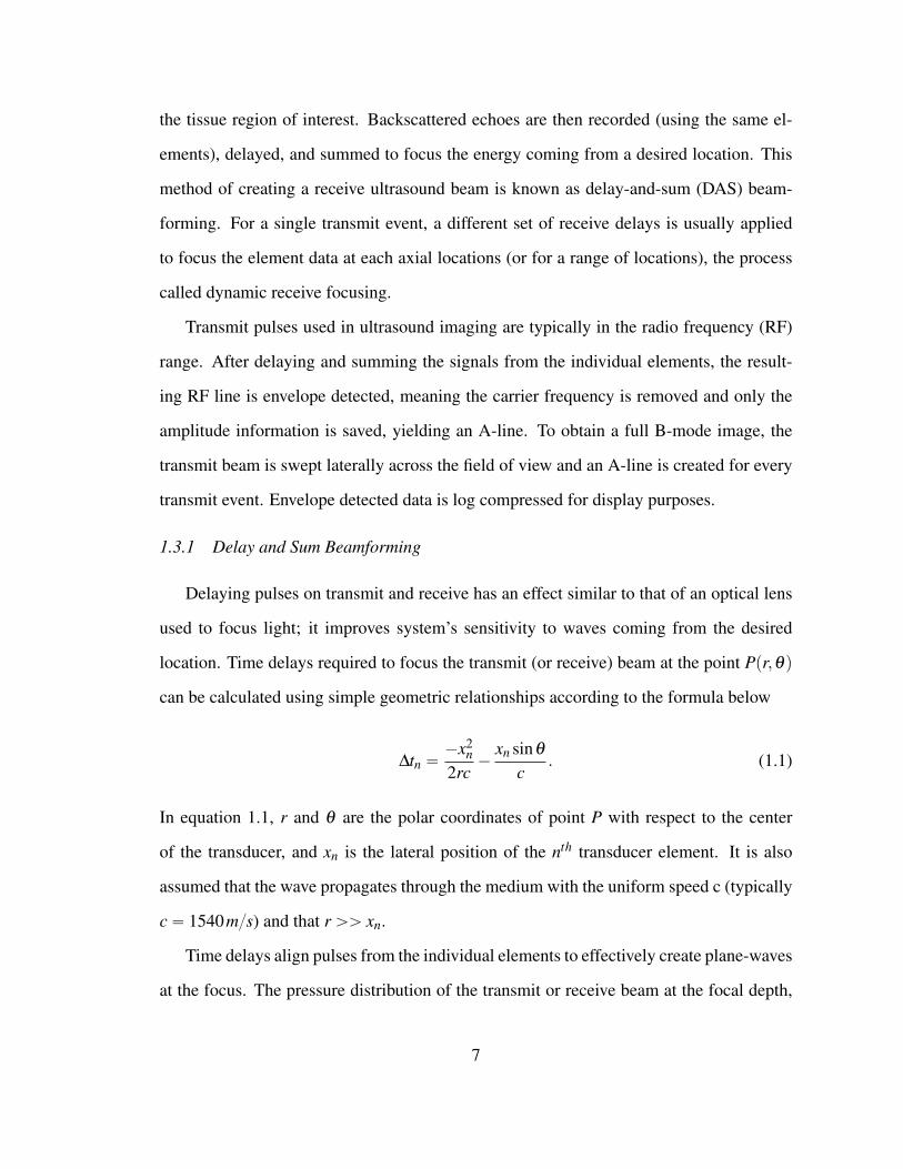
FIGURE 1.1: A simulated lateral PSF of an ultra-sound system that uses a 15 mm, 75-element, lin-ear array. Fractional bandwidth of the array is 0.5and the pulses are transmitted at 4 MHz center fre-quency. The width of the mainlobe (at half maxi-mum) is approximately 0.8 mm as predicted by theFourier transform relationship ( λ z
D ). The highestsidelobe levels are about -27 dB.
0 0.5 1 1.5 2 2.5−30
−20
−10
0
10
20
30
Time (us)
Voltage (
V)
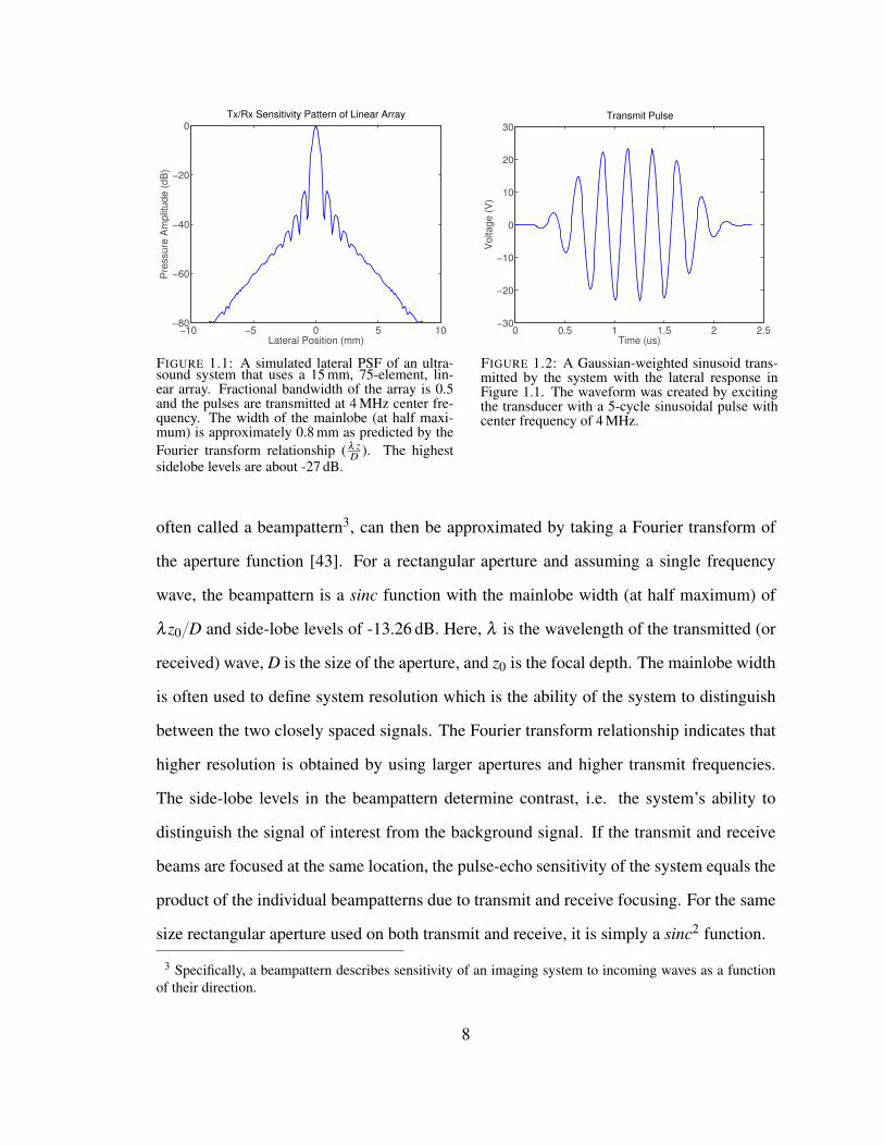
Transmit Pulse
FIGURE 1.2: A Gaussian-weighted sinusoid trans-mitted by the system with the lateral response inFigure 1.1. The waveform was created by excitingthe transducer with a 5-cycle sinusoidal pulse withcenter frequency of 4 MHz.
often called a beampattern3, can then be approximated by taking a Fourier transform of
the aperture function [43]. For a rectangular aperture and assuming a single frequency
wave, the beampattern is a sinc function with the mainlobe width (at half maximum) of
λ z0{D and side-lobe levels of -13.26 dB. Here, λ is the wavelength of the transmitted (or
received) wave, D is the size of the aperture, and z0 is the focal depth. The mainlobe width
is often used to define system resolution which is the ability of the system to distinguish
between the two closely spaced signals. The Fourier transform relationship indicates that
higher resolution is obtained by using larger apertures and higher transmit frequencies.
The side-lobe levels in the beampattern determine contrast, i.e. the system’s ability to
distinguish the signal of interest from the background signal. If the transmit and receive
beams are focused at the same location, the pulse-echo sensitivity of the system equals the
product of the individual beampatterns due to transmit and receive focusing. For the same
size rectangular aperture used on both transmit and receive, it is simply a sinc2 function.
3 Specifically, a beampattern describes sensitivity of an imaging system to incoming waves as a functionof their direction.
8

For a system employing DAS beamforming, pulse-echo sensitivity of the system can
also be directly measured by creating an image of a point target. The system response
to a point target, also known as the point spread function (PSF), is a two-dimensional
function that can be factored into separate lateral and axial responses at the focus. For
DAS beamforming, the lateral PSF is the same as beampattern. The simulated lateral
PSF of an ultrasound system employing a 15 mm, 75-element, linear array that has 0.5
fractional bandwidth and transmits at 4 MHz center-frequency is shown in Figure 1.1.
The PSF in the axial dimension is primarily determined by the shape of the transmit
pulse. For a Gaussian weighted sinusoid, the axial resolution at the focus is approximated
by nλ{2 where n is the number of transmitted cycles. A Gaussian weighted sinusoidal
pulse transmitted from the system with the lateral response plotted in Figure 1.1 is shown
in Figure 1.2.
1.3.2 Speckle Statistics
Assessing performance of an ultrasound system only in terms of its ability to detect a
point target has a limited applicability to in vivo imaging as there are few real point targets
in the human body. A more common scenario in imaging human tissue is to insonify lots
of sub-wavelength scatterers that cannot be resolved individually and whose amplitudes
and positions vary according to some probability distribution. Depending on their relative
phases for a particular realization, echoes from these scatterers add together at the face
of the transducer constructively or destructively, resulting in a pattern of dark and bright
regions called speckle, in the final ultrasound image. To characterize ultrasound images
(and system performance) in the presence of speckle, the use of 1st and 2nd order image
statistics is required.
Speckle patterns due to laser illumination have been extensively studied in optics [42]
and the results for the 1st and 2nd order speckle statistics have been extended to ultrasound
by several authors [13, 34, 116]. Wagner et al. [116] report speckle statistics for the
9

case of large number of randomly dispersed small scatterers (more than 10 scatterers per
resolution cell), assuming phases of the scatterers are uniformly distributed between 0 and
2π , and assuming the phase and amplitude of a single scatterer are independent of those
of other scatterers and of each other. In that case, the envelope-detected signal V can be
described by a Rayleigh probability distribution:
ppV q “Vσ2 exp
ˆ
´V 2
2σ2
˙
. (1.2)
In equation 1.2, σ2 is the variance of the complex signal recorded on the aperture and it
depends on the mean-square scattering amplitude of the particles in the imaged tissue. The
mean and the variance of V are given by:
xV y “´
π
2
¯1{2σ , (1.3a)
VarpV q “ˆ
4´π
2
˙
σ2, (1.3b)
where the angled brackets are used to designate the expectation operator. The quantity
xV y{pVarpV qq1{2 is called the speckle SNR and (under the previously stated assumptions)
is found to be a constant, 1.91. Thus, the speckle SNR is independent of scattering prop-
erties of imaged tissue or imaging system being used.
In addition to knowing the properties of signal at a single location in the speckle pat-
tern, it is important to know how these properties change over space. The autocorrelation
and the autocovariance of speckle are (interchangeably) used to convey the average simi-
larity between the signals measured at two locations in the speckle pattern, as a function
of their separation in space4. For the case of diffuse scatterers discussed above, Wagner et
al. [116] show that the autocovariance of complex amplitude (of ultrasound signal) can be
expressed in terms of the PSF of the system, gpxq, as follows:
Ccp∆xq “ a20 gp´∆xqbg˚p∆xq, (1.4)
4 The autocorrelation and the autocovariance are the same when both signals have zero mean.
10

where a0 is the average scattering strength of the particles, ∆x is the distance between the
locations x1 and x2 in the speckle pattern, and b is the convolution operator. When the
function in (1.4) is normalized by its maximum value, it is called the normalized autoco-
variance in c and is dependent only on the characteristics of the imaging system [116].
At the focus, the PSF, and therefore the autocovariance can be separated into factors
arising from lateral and axial directions:
Cc,x,zp∆x,∆zq “Cc,xp∆xq ¨Cc,zp∆zq. (1.5)
In equation 1.5, x and z are used to denote lateral and axial dimensions, respectively,
and Cc,xp∆xq and Cc,zp∆zq are the corresponding covariances. For a rectangular aperture
transmitting a Gaussian weighted sinusoid, the lateral and axial autocovariance functions
of complex amplitude are given by:
Cc,xp∆xq “ Kx sinc2pπ∆xD{λ z0qb sinc2
pπ∆xD{λ z0q, (1.6a)
Cc,zp∆zq “ Kz expp´p∆zq2{4σ2z q, (1.6b)
where D is the size of the aperture, λ is the wavelength of the sinusoid, z0 is the focal
depth, σz determines the width of the Gaussian envelope, and Kx and Kz are normalization
constants.
In practice, the autocovariance functions of signal magnitude and intensity (CV p∆xq
and CIp∆xq, respectively) are used rather than the autocovariance in complex amplitude as
the former two can be measured from a B-mode image. CV p∆xq and CIp∆xq are shown to
be very similar (no more than 3% difference), and can be computed from Ccp∆xq using
formulas presented in [87] and [116]. Measured normalized autocovariance functions for
lateral and axial directions are shown in Figures 1.3 and 1.4, respectively. Figures are
recreated from [106] and [115] and the original measurements were made on tissue mim-
icking phantoms. Distance is normalized in both plots to better convey the general shape
of the functions.
11
0 0.2 0.4 0.6 0.8 1 1.20
0.2
0.4
0.6
0.8
1
Distance (λz/D )
Norm
aliz
ed A
uto
covariance
Lateral Autocovariance of Speckle Pattern
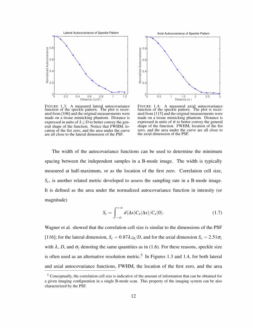
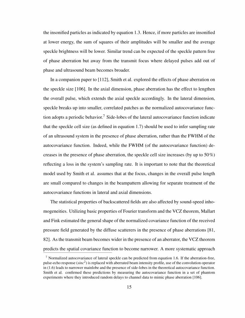
FIGURE 1.3: A measured lateral autocovariancefunction of the speckle pattern. The plot is recre-ated from [106] and the original measurements weremade on a tissue mimicking phantom. Distance isexpressed in units of λ z{D to better convey the gen-eral shape of the function. Notice that FWHM, lo-cation of the fist zero, and the area under the curveare all close to the lateral dimension of the PSF.
0 0.5 1 1.5 2 2.5 30
0.2
0.4
0.6
0.8
1
Distance (σ )
Norm
aliz
ed A
uto
covariance
Axial Autocovariance of Speckle Pattern
FIGURE 1.4: A measured axial autocovariancefunction of the speckle pattern. The plot is recre-ated from [115] and the original measurements weremade on a tissue mimicking phantom. Distance isexpressed in units of σ to better convey the generalshape of the function. FWHM, location of the fistzero, and the area under the curve are all close tothe axial dimension of the PSF.
The width of the autocovariance functions can be used to determine the minimum
spacing between the independent samples in a B-mode image. The width is typically
measured at half-maximum, or as the location of the first zero. Correlation cell size,
Sc, is another related metric developed to assess the sampling rate in a B-mode image.
It is defined as the area under the normalized autocovariance function in intensity (or
magnitude)
Sc “
ż `8
´8
dp∆xqCxp∆xq{Cxp0q. (1.7)
Wagner et al. showed that the correlation cell size is similar to the dimensions of the PSF
[116]; for the lateral dimension, Sc “ 0.87λ z0{D, and for the axial dimension Sc “ 2.51σz
with λ , D, and σz denoting the same quantities as in (1.6). For these reasons, speckle size
is often used as an alternative resolution metric.5 In Figures 1.3 and 1.4, for both lateral
and axial autocovariance functions, FWHM, the location of the first zero, and the area
5 Conceptually, the correlation cell size is indicative of the amount of information that can be obtained fora given imaging configuration in a single B-mode scan. This property of the imaging system can be alsocharacterized by the PSF.
12

under the curve are all similar to the corresponding dimension of the PSF.
1.3.3 Covariance of the Received Pressure Field
When diffuse scatterers in tissue are coupled with a transmit beam, they act as an
incoherent source6. Statistical properties of the wavefields emanating from incoherent
sources have been extensively studied in optics and a thorough review can be found in
[42]. In particular, the spatial coherence of a wavefield describes the average similarity
between two of its points as a function of their separation, and can be used to characterize
signals received across the aperture.
The Van Cittert-Zernike (VCZ) theorem predicts the coherence of the wavefield prop-
agating away from an incoherent source as the Fourier transform of that source’s intensity
distribution. Mallart and Fink applied the VCZ theorem to pulse-echo ultrasound [81],
and derived the expression for normalized covariance of the received pressure field when
imaging diffuse scatterers:
C1r f p∆xq “1
Cr f p0q
ż `8
´8
|Hpεq|2 exp„
´ j2π
zcp∆xεq
dε. (1.8)
In equation 1.8, the normalized covariance C1r f p∆xq is a function of distance between the
observation points x1 and x2, and H is the transmit beam amplitude. Normalized spatial
covariance is independent of focal length and transmit frequency and can be used to infer
shape of the transmit beam [82]. Utilizing properties of the Fourier transform, the covari-
ance can also be expressed in terms of the autocorrelation function of the transmit aperture.
When using a rectangular aperture of size D to insonify a region of diffuse scatterers, the
normalized covariance of received presure field is a triangle function with base 2D. It is
worth noting that these results are valid only when the observation points x1 and x2 are
located on the focused surface [81].
6 Incoherent source is a source that has statistical properties of white noise, i.e. its power spectrum is aconstant.
13

1.4 Beamforming Limitations and Image Degradation
Theory presented in Section 1.3 has been developed to characterize an ultrasound sys-
tem assuming ideal imaging conditions. In the following, we expand this theory to include
more realistic imaging scenarios. Changes of the beampattern, speckle statistics, and (spa-
tial) correlation of backscattered pressure fields are discussed to account for the presence
of phase aberration, reverberation, and limited acoustic window. Understanding of those
mechanisms is used to predict image degradation caused by the blocked elements.
1.4.1 Effects of Phase Aberration
The time-delay calculations in equation 1.1 assume that waves propagate through the
tissue with a uniform speed c. In the presence of sound-speed inhomogeneities, however,
different parts of wavefront will propagate at different speeds so the delayed pulses from
the individual elements will add out of phase at the focus. The beampattern in the presence
of phase aberration has been characterized through simulations [106, 110] and through in
vitro and in vivo experiments [89]. The results indicate widening and decrease in amplitude
of the mainlobe, and increased energy level in the tails of the function. A lateral shift of
the mainlobe (steering error) is also possible if the phase aberrator has a periodic structure
to it [106]. Following the definitions of lateral resolution and contrast outlined in section
1.3.1, these changes of the beampattern imply reduced lateral resolution and lower contrast
of the B-mode images in the presence of phase aberration.
Degradation of beampattern due to phase aberration also affects the 1st and 2nd order
speckle statistics. Trahey et al. showed through simulations and phantom experiments that
the average brightness of the speckle decreases with broadening of the ultrasound beam
(caused by phase aberration) [112]. As the energy of the beam shifts from mainlobe to tails
of the function, a larger number of diffuse scatterers is insonified at lower amplitude. The
mean value of speckle brightness xV y depends on the mean-square scattering amplitude of
14
the insonified particles as indicated by equation 1.3. Hence, if more particles are insonified
at lower energy, the sum of squares of their amplitudes will be smaller and the average
speckle brightness will be lower. Similar trend can be expected of the speckle pattern free
of phase aberration but away from the transmit focus where delayed pulses add out of
phase and ultrasound beam becomes broader.
In a companion paper to [112], Smith et al. explored the effects of phase aberration on
the speckle size [106]. In the axial dimension, phase aberration has the effect to lengthen
the overall pulse, which extends the axial speckle accordingly. In the lateral dimension,
speckle breaks up into smaller, correlated patches as the normalized autocovariance func-
tion adopts a periodic behavior.7 Side-lobes of the lateral autocovariance function indicate
that the speckle cell size (as defined in equation 1.7) should be used to infer sampling rate
of an ultrasound system in the presence of phase aberration, rather than the FWHM of the
autocovariance function. Indeed, while the FWHM (of the autocovariance function) de-
creases in the presence of phase aberration, the speckle cell size increases (by up to 50%)
reflecting a loss in the system’s sampling rate. It is important to note that the theoretical
model used by Smith et al. assumes that at the focus, changes in the overall pulse length
are small compared to changes in the beampattern allowing for separate treatment of the
autocovariance functions in lateral and axial dimensions.
The statistical properties of backscattered fields are also affected by sound-speed inho-
mogeneities. Utilizing basic properties of Fourier transform and the VCZ theorem, Mallart
and Fink estimated the general shape of the normalized covariance function of the received
pressure field generated by the diffuse scatterers in the presence of phase aberrations [81,
82]. As the transmit beam becomes wider in the presence of an aberrator, the VCZ theorem
predicts the spatial covariance function to become narrower. A more systematic approach
7 Normalized autocovariance of lateral speckle can be predicted from equation 1.6. If the aberration-free,pulse-echo response (sinc2) is replaced with aberrated beam intensity profile, use of the convolution operatorin (1.6) leads to narrower mainlobe and the presence of side-lobes in the theoretical autocovariance function.Smith et al. confirmed these predictions by measuring the autocovariance function in a set of phantomexperiments where they introduced random delays to channel data to mimic phase aberration [106].
15

was provided by Walker and Trahey [117] who modeled the aberrator as a near-field phase
screen and derived the following expression for the normalized covariance of the pressure
field received from a speckle generating target
C1r f p fzq “
ş`8
´8T pXaqT ˚pXa´∆XqdXa
ş`8
´8T pXaqT ˚pXaqdXa
ˆ exp`
p´2π fzq2pRττp0q´Rττp∆Xqq
˘
. (1.9)
In equation 1.9, C1r f is a function of transmit frequency fz, T pXq is the transmit aperture
function, and Rττ is the spatial autocovariance of the aberrator. This model showed excel-
lent agreement with the simulation results predicting a sharp drop in the spatial covariance
function in the presence of a severe aberrator [117].
1.4.2 Reverberation Clutter
Tissue inhomogeneities can also lead to reverberation (multipathing), which is another
significant source of image degradation [14, 67, 99]. Layered tissue structures or defuse
inhomogeneities can cause waves to undergo many scattering events before impinging on
the transducer surface. If waves resonate between the parallel tissue interfaces (such as
those found in a vessel wall), received echoes will write bright periodic bands over the
signal of interest. If waves insonify a region with diffuse inhomogeneities, or if there is
a large number of non-parallel interfaces (e.g. fat-connective tissue interfaces in obese
individuals), receive channels will be corrupted with a less-coherent noise causing a sharp
decorrelation of signal across the aperture [66]. This type of noise appears in images as
diffuse haze and is called clutter.
While many methods for clutter reduction have been proposed recently, few analytic-
form models of clutter appear in the ultrasound literature. In [24], Dahl et al. modeled
clutter as additive white-noise, filtered with the transducer impulse response. In particu-
lar, they used FIELD II simulations to assess performance of short-lag spatial coherence
(SLSC) imaging in lesion detection in the presence of clutter; the applied clutter model
16

yielded contrast and CNR trends that were in good agreement with the in vivo results [59].
Byram et al. modeled echoes from multipathing as linear-frequency-modulated sinusoids
(i.e. chirps) in the aperture domain, and subsequently removed them from the overall sig-
nal to successfully reduce clutter in simulated and in vivo images [14, 15]. Pinton et al.
[99] estimated image degradation due to clutter by numerically simulating wave propaga-
tion through a layer of abdomen. Simulations were based on the full-wave equation, which
accounts for the effects of non-linearity, attenuation, and reverberation. By controling the
density and speed-of-sound maps, the effects of reverberation and phase aberration could
be studied independently. Removing the sources of reverberation clutter recovered CNR
of the anechoic lesion located at 3.5 cm depth by as much as 30 % (of the control value
obtained from the homogenous simulation); CNR of the anechoic lesion at 5 cm depth was
increased by 16 % of its control value.
1.4.3 Limited Acoustic Window
Beam degradation due to a limited acoustic window can be predicted by using a Fourier
transform relationship between the pressure distributions at the face of the transducer and
at the focus, as outlined in section 1.3.1. In particular, if an acoustic obstacle effectively
prevents parts of the array from transmitting and/or receiving acoustic pulses, the degraded
beampattern can be estimated by taking a Fourier transform of the newly-formed sparse-
aperture function. A corrupt beampattern typically has higher side-lobe levels than the
beampattern due to fully functional array. Additionally, if end-elements of the array are
blocked, the overall aperture size is reduced and a wider mainlobe results [70].
Ramsdale and Howerton addressed a similar problem of beampattern degradation due
to element failure in sonar arrays [101]. They found that the peak sidelobe level of the
average beampattern is proportional to the ratio of the sum of the weights of the inoperative
17
elements to the sum of the weights of the operative elements
SSLxPpθqypmaxq9ř
anpinoperativeqř
anpoperativeq. (1.10)
Using equation 1.10, Ramsdale and Howerton found that a single faulty element leads
to an increase in the maximum sidelobe level that corresponds to a 30˝ maximum phase
error across the array (approximately 3.5dB). As the number of faulty elements increases,
maximum sidelobe level increases and the shape of the sidelobes starts to depend more on
the beampattern of the inoperative part of the aperture [101].
1.4.4 Image Degradation due to Blocked Elements
As stated previously, the loss of image quality in the presence of blocked elements
can be explained as a combination of two factors, sound-speed inhomogeneities and a
limited acoustic window. Both factors lead to broadening of the ultrasound beam and
increased side-lobe levels, which in turn, causes a loss of resolution and decreased visi-
bility of anechoic/hypoechoic targets. Further, the 1st and 2nd order speckle statistics are
expected to follow the changes in the beampattern outlined in Section 1.4.1. Speckle is
expected to break up into smaller, correlated patches and its average brightness should
be lower.8 Backscattered echoes should rapidly decorrelate across the receive aperture as
the signals from the blocked elements experience attenuation, a random phase shift, and
increased amount of reverberation noise due to acoustic-impedance mismatch between the
soft tissue and bone. The nearest-neighbor cross-correlation between the blocked elements
should be particularly low. Acoustic noise due to reverberation is expected to appear as
clutter in the near-field region of the final B-mode image.
8 The normalized autocovariance function of lateral speckle is expected to exhibit a periodic behavior dueto increased side-lobe levels in the beampattern. Therefore, speckle cell size (defined in (1.7)) should beused to assess the number of independent samples in a degraded B-mode image.
18

1.5 Adaptive Imaging Methods
The beampattern shown in section 1.3.1 assumes uniform weighting of the individual
channel signals. To reduce the width of the mainlobe or to decrease the sidelobe levels
different weighting (apodization) schemes can be applied to the channel data. When the
weights are independent of the channel data (conventional beamforming), there is a trade-
off between the mainlobe width and the sidelobe levels of the resulting beampattern. Some
of the typically used (non-adaptive) apodization functions are Gaussian, Hamming, Dolph-
Chebyshev, Hann, and Kaiser windows [60].9
System sensitivity (in the lateral dimension) can be further improved if the channel
weights are allowed to change with the received signals, process known as adaptive beam-
forming. Adaptive weights are usually chosen to minimize some cost function subject
to a constraint. For example, in a Minimum Variance Distortionless Response (MVDR)
beamformer, weights are chosen that minimize the total output power while keeping the
response to signal coming from a desired direction unchanged [60]. In other words, the
weight vector wMVDR is a solution to the following constrained optimization problem
minw pw`Rwq subject to e`w“ 1 ,
where R is the cross-correlation matrix of the received channel data, e is a so-called steer-
ing vector that specifies the direction of the desired signal, and ` stands for the conjugate
transpose operator. Using the method of Lagrange multiplier wMV DR is calculated as
wMVDR “R´1e
e`R´1e. (1.11)
Adaptive weights defined by (1.11) result in suppression of interference (signal coming
from undesired direction) while preserving the signal of interest. MVDR is the most ef-
fective in suppressing isolated, point-like targets that are not in the immediate proximity9 Applying weights to the individual channel data can be conceptualized as a spatial filtering operation.
Therefore, windowing functions that are used to filter time-series data can be also used for aperture apodiza-tion.
19

of the desired signal. In the presence of distributed targets, the performance of MVDR
approaches that of DAS beamforming.
The adaptive imaging methods can be also used to improve image quality in the pres-
ence of phase aberration, clutter, and blocked or missing elements. Some of the most
commonly used such methods are reviewed in the remainder of this section.
1.5.1 Phase Aberration Correction
Several methods have been developed to improve a beampattern in the presence of
phase aberration [23, 32, 35, 38, 76, 77, 91, 93, 123], and they can be grouped based on
the model of the aberrator they employ. When the aberrator is modeled as a thin screen
at the face of the transducer (the so-called near-field phase-screen model), the received
waveforms are assumed to be time-delayed versions of their non-aberrated counterparts.
If this assumption is true, the ideal beampattern can be recovered by estimating the tissue-
induced time-delays and applying them to the individual channel signals so they can be
summed in phase.
Liu et al. [77] applied the near-field phase-screen model to find a least-squares (LS)
estimate of the arrival-time profiles for the wavefronts that propagated through the excised
sections of human abdomen. Specifically, they measured the (tissue-induced) time-delays
between the neighbouring channels from the peak of their cross-correlation functions. A
large number of delay measurements (four nearest-neighbour delay values per channel)
allowed them to model a highly over-determined system and compute an LS estimate of
the arrival-time10 for each channel. The corrected beampatterns showed the -10 dB effec-
tive width that is on average 30 % smaller than the effective width of the non-compensated
beampattern, and is 4 % larger than the effective width of the ideal (non-aberrated) beam-
pattern. The average ratio of the energy outside of the -10 dB effective-width-region to
the energy inside the region is 1.81 for the uncompensated, 0.93 for the compensated, and
10 The arrival time for a channel can be thought of as a time-delay relative to the reference waveform.
20

0.35 for the ideal beampatterns. A similar LS-based phase-aberration correction technique
was successfully applied in [23, 30, 40], but in combination with the property of phase
enclosure, which states that the signal-phases (or time-delays) along any closed path on
the aperture have to add to zero. If the system of equations is allowed to include the delay
measurements at higher lags (in addition to neighbouring elements), phase enclosure can
provide for multiple measurements for any pair of channels in the aperture which increases
accuracy of the arrival-time estimates.
Under a more realistic imaging scenario, parts of the wavefront experience time-shifts
at some distance away from the transducer surface. As the time-shifted wavefront con-
tinues to propagate, the amplitude and shape distortions develop and the received signals
lose similarity (coherence) across the channels. In that case, estimating the delays from
the channel data is more difficult, and delaying the individual channel signals alone is
not sufficient to fully recover the beampattern. Indeed, in [76], Liu et al. showed that the
phase-aberration correction can be improved if the phase-screen is modeled at some (axial)
distance away from the transducer, and the received waveforms are back-propagated to the
phase-screen location before estimating the time-delays. The axial location of the phase-
screen was determined where the (back-propagated) signals showed the highest degree of
similarity along the array dimension. For the beampatterns measured on 14 samples of hu-
man abdomen, the -10 dB peripheral energy ratio decreased on average from 0.63 for the
time-shift compensation alone to 0.47 when the time-shift compensation was preceeded
by back-propagation.
For the time-delay focusing techniques to be effective, speed-of-sound inhomogeneities
have to be confined to a thin region, i.e. they have to meet the assumptions of the phase-
screen model. If the speed-of-sound inhomogeneities are distributed throughout the medium,
the shape of the propagating wave gets distorted through refraction, diffraction, and mul-
tiscattering, and the adaptive channel-delays can no longer improve focusing. To achieve
optimal focusing in the presence of such an aberrator, Fink et al. proposed the method of
21

time-reversal mirror (TRM) [32, 123]. Specifically, if a point-like source is placed at the
(desired) target location, the aberrated wavefronts can be recorded on the aperture, time-
reversed, and re-emitted. The energy at the target location is then maximized since the
time-reversal of the aberrated waveform allows the inhomogenous transfer function be-
tween the array and the target to act as a matched filter. Corrected beampatterns measured
in the phantom experiments in [123] demonstrate that the TRM can achieve high-quality
focus for different positions and shapes of the aberrator. While the TRM is insensitive
to the aberrator geometry/structure, it requires the presence of a point source at the focus
making its in vivo application difficult.
1.5.2 Clutter Suppression via Coherence-based Imaging Methods
Low coherence of ultrasound signals across the receive aperture can be an indicator
of low image quality. When a region of diffuse scatterers is insonified with a rectangular
aperture of size D, the (spatial) covariance of receive pressure fields is expected to be a
triangle function with base 2D (section 1.3.3). However, the spatial covariance decreases
at a faster rate in the presence of phase aberration and reverberation (section 1.4). The
idea behind most of coherence-based imaging methods is to identify and suppress the
incoherent portions of the signal in order to reduce the effects of phase aberration and
reverberation.
Some of the metrics based on the receive-signal coherence are listed bellow:
1) the Coherence Factor - defined as as a ratio of the coherent sum to the incoher-
ent sum of the received echoes, it was designed to measure the focus quality of
an ultrasound imaging system and to measure the performance of phase-aberration
correction algorithms [82],
2) the Waveform Similarity Factor - a metric similar to the Coherence Factor, it was in-
troduced to measure similarity of the received waveforms along the array dimension,
as they were back-propagated to determine the axial location of the phase screen and
22

to perform subsequent aberration correction [76],
3) the Generalized Coherence Factor - similar to the Coherence Factor and developed
to suppress phase-aberrated signals [71],
4) the Phase Coherence Factor and the Sign Coherence Factor - the two metrics were
based on the variance of phase of the received echoes across the aperture, and were
intended to reduce the off-axis scattering [16].
The latter three metrics were used to weight B-mode images on a pixel-by-pixel bases in
order to reduce the effects of phase aberration.
In an alternative approach, Walker and Trahey developed a translating aperture method
that uses multiple transmits to improve correlation of speckle across the receive channels
[117]. Specifically, if the aperture is translated between the transmits by the same amount
and in direction opposite to that of a desired receive-element lag, the decorrelation of
speckle due to (transmit-receive) geometry is eliminated, and only decorrelation due to
aberration remains. For the phase aberration correction schemes that rely on the near-
field phase-screen model, this technique can improve the estimates of tissue-induced time
delays resulting in a higher quality of corrected images.
Lediju et al. have recently developed a beamforming method called Short-Lag Spatial
Coherence (SLSC) imaging [66] that suppresses the incoherent portion of received echoes
and has the potential to reduce clutter. Unlike the previously described coherence-based
metrics that are used to weight B-mode images, SLSC imaging relies solely on the coher-
ence of back-scattered echoes, and not on their magnitude. Specifically, to determine the
value of a pixel in SLSC image, the spatial coherence curve is computed from the individ-
ual channel signals and integrated over the region of low lags. The exact implementation
of the SLSC method on 1-D and 2-D arrays is described in sections 2.2.1 and 3.2.1, re-
spectively. Simulated and in vivo SLSC images look comparable to conventional B-mode
images under noise-free conditions, and show dramatically improved visualization of ane-
choic and hypoehoic targets in a noisy environment [24, 25]. The beamforming principles
23

behind the SLSC imaging have been also applied to harmonic signals (the method called
Harmonic Spatial Coherence Imaging or HSCI [25]), and towards power Doppler imaging
for improved flow detection (Coherent Flow Power Doppler or CFPD [72]).
Other (non-coherence-based) approaches for clutter reduction include harmonic (DAS)
imaging [5, 19], chirp-based signal decomposition [14, 15], and motion-based approach
to clutter reduction [69].
1.5.3 Compensation for the Blocked and Missing Elements
To improve the beampattern in the presence of blocked or inoperable elements, the
constrained optimization approach can be used to solve for the weights on the remaining
elements. Er and Hui proposed to minimize the mean-square error in the mainlobe region11
while keeping the mean-square sidelobe levels within some user-defined boundary ε and
forcing the weights of inoperable elements to zero [28]. As indicated by the simulated
beampatterns, the resulting weight vector effectivelly reduces sidelobes for a small number
of faulty elements. However, since the weights are not adaptive (despite being a solution
to a constrained optimization problem)12, the DAS sensitivity pattern sets the upper limit
on the method’s performance.
A common way to adaptively compensate the array beampattern in the presence of in-
operable elements is to interpolate the signals on those elements. In that case, a constrained
optimization problem can be formulated as
minp pp`Q`minQminpq subject to }L`p´xoperable}22 ă ε ,
with the solution given by
p“ pQminQ`min`µLL`q´1µLxoperable . (1.12)
11 Here, the error is defined as a difference between the actual array response and a desired array response.12 The weights do not depend on the received signals and the locations of the inoperable elements are knowna priori.
24
In other words, a full array data-set p is reconstructed such that its noise component is
minimized while keeping the distortion of the signals from the operable elements xoperable
within some value ε . In equation 1.12, columns of Qmin are eigenvectors that define the
noise-subspace of the channel cross-correlation matrix R, L is a selection matrix that spec-
ifies the positions of the operable elements, and the scalar parameter µ controls the amount
of noise suppression. Kazanci and Krolik modified this approach by solving the optimiza-
tion problem in the beam-space rather than in the element-space and called it Beam-space
Adaptive Channel Compensation (BACC) [61]. Assuming that the highest receive-beam
sidelobes occur within the mainlobe of the transmit-beam and that the number of receive
beams needs not be large, transforming from element-space to beam-space significantly
improves computational efficacy of the algorithm. Simulation results show that BACC
is capable of suppressing sidelobes and improving target detectability in the presence of
distributed targets (clutter) or directional interference.
As discussed previously (section 1.4.3), the effects of blocked elements on the beam-
pattern are similar to those caused by inoperable elements. Nevertheless, instead of trying
to correct the distorted beampattern, Li et al. developed a method that compensates for
the blocked elements by directly suppressing the contributions from the off-axis scatterers
[70]. For every transmit beam, multiple receive beams are created (via DAS beamform-
ing) to measure the source profile. Measured source profile can be represented by the
convolution sum of the true source profile and the beampattern (degraded by the blocked
elements)
Ba“ x (1.13)
In equation 1.13, each column of matrix B is a degraded beampattern centered around the
direction of the ith source ∆i, vector a contains the complex amplitudes of the scattering
sources (targets), and vector x is the measured complex source profile. The direction
and amplitude of the most dominant targets can then be estimated as the solution to the
25

following minimization problem
∆i , a“min}Ba´x}2 . (1.14)
With a and ∆i’s known, the undesired sidelobe contributions from the off-axis scatterers
are easily removed from (the receive beam at) the transmit direction.
To construct the model in (1.13), Li et al. made the following assumptions:
1) the medium is insonified with a continuous wave so the degraded beampattern can
be approximated by the Fourier transform of the sparse-aperture function where the
blocked elements are weighted by zero and the active elements are weighted by one,
2) the number and position of blocked elements are known for each imaged point al-
lowing matrix B to be updated accordingly, and
3) the targets can be presented by delta functions.
In addition, the estimates of a are obtained via the total least squares (TLS) method and as
such, are robust to the imperfections in the model.13 The method was shown to be effec-
tive in improving phantom images of point-targets and distributed targets for a reasonable
number of blocked elements. However, in the in vivo setting, the targets would have to
be classified before the method could be used since the TLS is not adequate for bimodal
targets and anechoic regions.
1.6 Imaging with Matrix Arrays
The conventional ultrasound system described in section 1.3 uses a 1-D array of el-
ements to scan a single plane in tissue. Electronic delays are applied to the individual
elements to steer and focus ultrasound beam at the desired locations in the azimuth plane.
In the elevation plane, a cylindrical ultrasound lens covering the aperture provides a fixed
focus.13 Unlike the traditional least squares method which assumes that the model is correct and the error isconfined to the observation vector, the method of total least squares allows for error to reside in both modeland measurements. This improves robustness of the estimates but increases computational complexity of thealgorithm.
26

This configuration imposes several limitations on image quality and potential applica-
tions. The small elevation dimension of the array (typically less than 2 cm), in combination
with the fixed focus yields a relatively thick B-mode slice and significant contributions
from the out-of-plane scatterers. Outside of the fixed focus, elevation resolution can be up
to several times larger than lateral resolution, making the ultrasound beam highly asym-
metric and limiting the detection rate of small targets. Simulation studies have compared
the performance of 1-D and 2-D arrays when imaging small hypoechoic lesions, and re-
ported a loss of target contrast for images created with the linear array [114]. Further, some
adaptive imaging algorithms, such as most of the phase-aberration correction schemes and
SLSC imaging show limited success when implemented on a 1-D array because the quanti-
ties they estimate (a phase-screen aberrator and the normalized spatial covariance, respec-
tively) usually vary along both dimensions of the aperture [31, 54]. Completely averaging
one of the dimensions degrades the accuracy of the estimate.
Arrays that have at least three rows of elements can also focus an ultrasound beam in
elevation plane, with varying degrees of freedom. Following the nomenclature in [122],
a 1.5-D array can apply dynamic focusing in the elevation dimension, but only along the
center-axis of the transducer. 1.5-D arrays typically have three to five rows of elements,
and have demonstrated reduced slice thickness and a more uniform beam profile in the ele-
vation direction compared to linear arrays [22, 122]. In addition to variable depth focusing,
a 1.75-D array can slightly deflect a beam in the elevation plane. Some 1.75-D arrays can
steer up to 30 degrees in elevation while maintaining a reasonable beamwidth [47]. Al-
though 1.75-D arrays contain a limited number of element rows (usually no more than
10), they proved successful in measuring and correcting for 2-D phase aberration profiles
[23, 30, 31, 39]. In simulation and in phantom experiments, Fernandez et al. [31] showed
that as the aperture sampling along the elevation dimension increases, the accuracy of a
2-D aberration profile improves, with as few as three rows of elements bringing significant
improvements in accuracy over a linear array. Hyun et al. showed similar trends relating
27
aperture sampling (in either dimensions) and the quality of SLSC images [54].
2-D arrays can achieve full electronic steering, focusing, and aperture selection in the
elevation dimension allowing them to scan complete 3-D volumes at high speeds [100,
105, 107]. To this end, they usually have a similar number of elements in both dimensions.
One of the first 2-D arrays was a 17-by-17 phased array developed as a part of a real-time
volumetric system at Duke University [100, 105]. Due to a limited number of system
channels (32 on transmit and 32 on receive), active elements had to be sparsed through
the aperture. Different array geometries, such as Mills cross, circular aperture, and com-
bination of the two were tested on transmit and receive to optimize the 2-D pulsed-echo
response.
Since then, 2-D arrays have been developed to have thousands of elements and the
sparse sampling methods have been used widely to pass the aperture data to a limited
number of system channels [4, 12, 27, 53, 74, 78, 119, 124]. Typically, the active ele-
ments are distributed so to minimize the mainlobe width while keeping the grating lobes
under a reasonable level. Lockwood et al. [78] achieved this by choosing transmit and
receive apertures that are analogous to the stationary and sliding parts of the Vernier scale
(so-called Vernier arrays). The ’sliding’ aperture has less elements and a slightly smaller
element spacing than the ’stationary’ aperture, so that the resultant effective aperture ap-
proximates that of a fully populated array. In another approach, Davidsen et al. [27]
explored performance of randomly populated sparse arrays; a random array with Gaus-
sian distribution on transmit and uniform distribution on receive showed improved resolu-
tion and depth-of-field compared to standard Mills cross design and a random array with
uniform distribution on both transmit and receive. A comprehensive overview of sparse
periodic designs based on different combinations of symmetry is presented in [4], includ-
ing symmetric and asymmetric periodicity, and periodicity along x-axis and y-axis, along
diagonals, and along radii.
To allow use of all elements in a 2-D aperture while accommodating for a limited
28

number of systems channels, most of modern commercial 2-D arrays employ subaperture
beamforming in the transducer handle. ASICs in the handle perform delay-and-sum beam-
forming on small groups of elements and partially beamformed data is passed on to system
channels for further processing; this reduces the number of signals the scanner would have
to process from several thousand to typically less then two hundred. While subaperture
electronics brings down cable weights and overall system cost, they cause a significant
loss of sensitivity in 2-D arrays [79]. In addition, the resultant inability to access radio-
frequency (RF) data for each element inhibits the realization of many techniques requir-
ing custom transmit sequences or advanced aperture-domain signal processing, including
phase aberration correction and adaptive beamforming.
Small element size, electronics in the transducer handle, and use of broad transmit
beam are the main causes of reduced sensitivity when imaging with 2-D arrays. Specif-
ically, elements of a matrix array are small and therefore have high impedance (or low
capacitance) resulting in poor impedance match with front-end electronics; this causes
both low transmit power and low receive sensitivity [41]. In addition, it requires ASICs
for partial-beamforming to be as close to elements as possible to minimize parasitic capac-
itance [79]. Electronics in the handle therefore have to be small and can operate only in
low voltage regime, which further limits sensitivity of the array. Electronics in the handle
also couples energy from an active element to the surrounding elements resulting in un-
desirable cross-talk [113]. Finally, to scan full volumes at real-time rates, broad transmit
beams are typically used causing a loss in transmit resolution.
Despite their design limitations, matrix arrays offer a unique opportunity to visualize
structures in three dimensions, non-invasively, and in real-time. This hold tremendous
potential for many clinical applications including volume estimation of heart chambers
and tumor masses, volumetric angle-independent flow imaging, and 3-D motion tracking
of heart walls and valves. Beamforming methods that would mitigate loss of sensitivity
and reduce the rate of suboptimal 3-D exams would secure a wider use of matrix arrays in
29

clinical practice.
30
2
Short-Lag Spatial Coherence Imaging on 1-DArrays: Results of a Pilot Study on Human Livers
2.1 Introduction
Ultrasound is commonly used for surveillance and diagnosis of liver diseases because
of its high specificity (75-98%), relatively low cost, and lack of ionizing radiation [8, 18,
64, 88, 90, 103]. In many hospitals, asymptomatic patients with an incidental elevation of
liver enzymes receive periodic abdominal ultrasound scans in an attempt to diagnose early
onset of non-alcoholic fatty liver disease (NAFLD), the most common form of liver dis-
ease [63, 88]. Hepatorenal echo contrast, liver tissue brightness, and vascular blurring are
indicators typically used to detect and stage NAFLD [88]. In a similar manner, the Amer-
ican Association for the Study of Liver Diseases has recommended periodic ultrasound
exams as a part of standard surveillance procedure for hepatocellular carcinoma (HCC)
[10].
For both NAFLD and HCC, the role of ultrasound in diagnosing and staging the disease
is sometimes limited by inadequate image quality. Most of the patients that are at risk of
or are already suffering from NAFLD are categorized as overweight or obese (based on
31
their body mass index) and may yield low quality images. A study done on morbidly
obese patients reports the sensitivity of ultrasound in diagnosing hepatic steatosis (fatty
liver disease) to be only 49.1% [90]. The growing population of overweight and obese
patients is also under increased risk of developing HCC. The American Association for the
Study of Liver Diseases acknowledges that these patients are often not good candidates for
HCC surveillance [10], where the reported values for sensitivity are as low as 65% [18].
The body habitus of overweight and obese patients introduces a variety of challenges in
ultrasonic imaging, one of which is an increased level of acoustical noise known as clutter.
Clutter is a significant reason for diminished quality of ultrasound images of the liver
[68, 97]. It appears as an overlaying haze or fill-in that obscures in vivo structures such
as lesions and blood vessels and leads to inadequate visualization of liver anatomy and
function. The three main sources of clutter that have been identified are phase aberration,
reverberation among tissue layers, and off-axis scattering [97]. Many of these sources of
clutter are present in overweight and obese individuals due to thick layers of subcutaneous
fat and fat/connective tissue interfaces. As a result, there is a growing clinical need for
ultrasound imaging techniques that would reduce clutter or improve image quality and
allow for more patients to be effectively surveyed for liver diseases such as NAFLD or
HCC.
Harmonic imaging and various phase aberration correction methods are examples of
techniques developed to reduce clutter. Harmonic imaging is based on nonlinear wave
propagation, which generates frequency components at integer multiples of the transmitted
frequency. This phenomenon is negligible close to the surface of the transducer, which re-
sults in a reduction of near-field reverberation clutter [5, 19]. However, harmonic imaging
does not suppress clutter originating from phase aberration; in fact, it is more susceptible
to phase aberration than fundamental B-mode due to the higher receive frequency [97].
Phase aberration correction methods can reduce side-lobe levels and the effects of off-axis
scattering [32, 35, 76, 92]. However, their potential to improve quality of fundamental
32

B-mode images is limited because of overlaying reverberation clutter [97].
Adaptive imaging methods based on spatial coherence of the pressure field present an
alternative approach to improving image quality. Walker and Trahey developed a translat-
ing aperture technique to improve speckle correlation and thus facilitate near-field phase
aberration correction [117]. Mallart and Fink introduced the Coherence Factor, defined
as a ratio of the coherent sum to the incoherent sum of the received echoes, in an attempt
to quantify focusing characteristics of ultrasonic imaging systems [82]. The Generalized
Coherence Factor [71] is a coherence measurement similar to the Coherence Factor and
was developed primarily to suppress phase-aberrated signals. The Phase Coherence Factor
and the Sign Coherence Factor are based on the variance of phase of the received echoes
across the aperture and are intended to reduce the off-axis scattering [16]. The General-
ized Coherence Factor, Phase Coherence Factor, and Sign Coherence Factor are all used
to weight the B-mode on a pixel-by-pixel basis in order to improve B-mode image quality.
We have recently developed a beamforming method called Short-Lag Spatial Coher-
ence (SLSC) imaging [66] that suppresses the incoherent portion of the backscattered
ultrasound field and has the potential to reduce clutter. We have also adapted SLSC imag-
ing to the backscattered harmonic field and called it Harmonic Spatial Coherence Imag-
ing (HSCI) [25]. Both SLSC and HSCI are based purely on the spatial coherence of
backscattered echoes and do not depend on the echo magnitude. We have demonstrated
through simulations that SLSC imaging performs as well as conventional B-mode imag-
ing in detecting lesions under noise-free conditions while it dramatically improves lesion
detectability in a noisy environment [24]. Sample SLSC and HSCI images of in vivo liver,
heart, and kidney also show improved visibility of targets and indicate that SLSC and
HSCI could have significant clinical impact [25]. In this chapter, we report the results of
a pilot patient study conducted to assess the clinical performance of SLSC and HSCI in
liver imaging. Image metrics (contrast and CNR) are computed for fundamental B-mode,
harmonic B-mode, SLSC, and HSCI images to quantify and compare visibility of in vivo
33
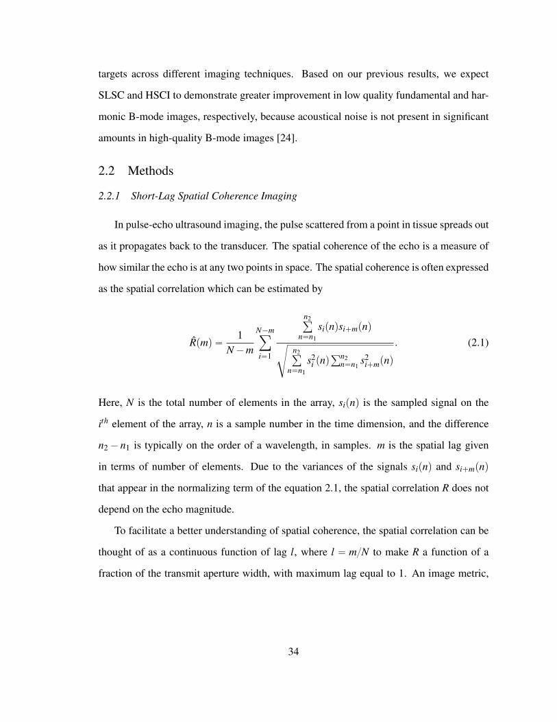
targets across different imaging techniques. Based on our previous results, we expect
SLSC and HSCI to demonstrate greater improvement in low quality fundamental and har-
monic B-mode images, respectively, because acoustical noise is not present in significant
amounts in high-quality B-mode images [24].
2.2 Methods
2.2.1 Short-Lag Spatial Coherence Imaging
In pulse-echo ultrasound imaging, the pulse scattered from a point in tissue spreads out
as it propagates back to the transducer. The spatial coherence of the echo is a measure of
how similar the echo is at any two points in space. The spatial coherence is often expressed
as the spatial correlation which can be estimated by
Rpmq “1
N´m
N´mÿ
i“1
n2ř
n“n1
sipnqsi`mpnqd
n2ř
n“n1
s2i pnq
řn2n“n1
s2i`mpnq
. (2.1)
Here, N is the total number of elements in the array, sipnq is the sampled signal on the
ith element of the array, n is a sample number in the time dimension, and the difference
n2´ n1 is typically on the order of a wavelength, in samples. m is the spatial lag given
in terms of number of elements. Due to the variances of the signals sipnq and si`mpnq
that appear in the normalizing term of the equation 2.1, the spatial correlation R does not
depend on the echo magnitude.
To facilitate a better understanding of spatial coherence, the spatial correlation can be
thought of as a continuous function of lag l, where l “ m{N to make R a function of a
fraction of the transmit aperture width, with maximum lag equal to 1. An image metric,
34
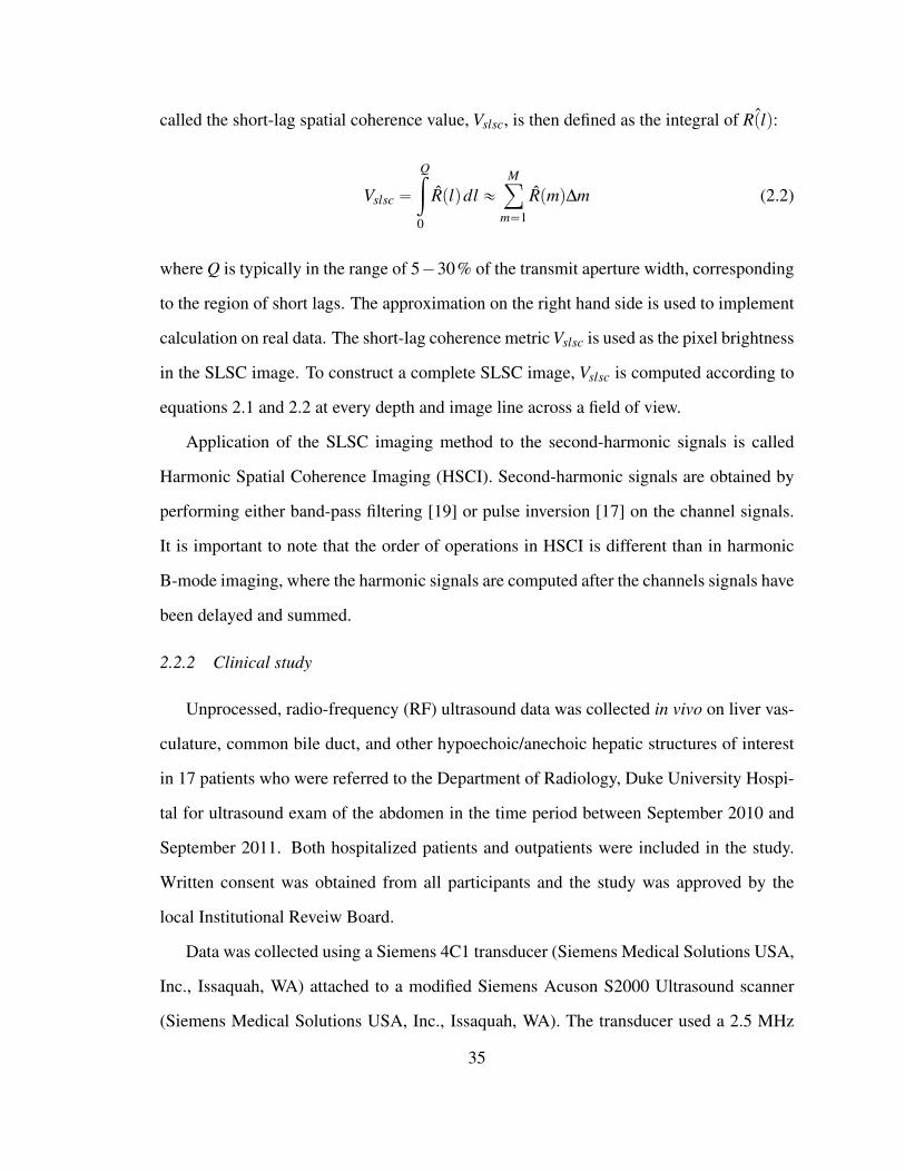
called the short-lag spatial coherence value, Vslsc, is then defined as the integral of ˆRplq:
Vslsc “
Qż
0
Rplqdl «Mÿ
m“1
Rpmq∆m (2.2)
where Q is typically in the range of 5´30% of the transmit aperture width, corresponding
to the region of short lags. The approximation on the right hand side is used to implement
calculation on real data. The short-lag coherence metric Vslsc is used as the pixel brightness
in the SLSC image. To construct a complete SLSC image, Vslsc is computed according to
equations 2.1 and 2.2 at every depth and image line across a field of view.
Application of the SLSC imaging method to the second-harmonic signals is called
Harmonic Spatial Coherence Imaging (HSCI). Second-harmonic signals are obtained by
performing either band-pass filtering [19] or pulse inversion [17] on the channel signals.
It is important to note that the order of operations in HSCI is different than in harmonic
B-mode imaging, where the harmonic signals are computed after the channels signals have
been delayed and summed.
2.2.2 Clinical study
Unprocessed, radio-frequency (RF) ultrasound data was collected in vivo on liver vas-
culature, common bile duct, and other hypoechoic/anechoic hepatic structures of interest
in 17 patients who were referred to the Department of Radiology, Duke University Hospi-
tal for ultrasound exam of the abdomen in the time period between September 2010 and
September 2011. Both hospitalized patients and outpatients were included in the study.
Written consent was obtained from all participants and the study was approved by the
local Institutional Reveiw Board.
Data was collected using a Siemens 4C1 transducer (Siemens Medical Solutions USA,
Inc., Issaquah, WA) attached to a modified Siemens Acuson S2000 Ultrasound scanner
(Siemens Medical Solutions USA, Inc., Issaquah, WA). The transducer used a 2.5 MHz
35

center frequency with a 60 % fractional bandwidth. The individual channel signals needed
to create SLSC and HSCI images were recorded using a custom synthetic-receive-aperture
sequence in combination with the Axius DirectTM Ultrasound Research Interface [11]. The
transducer had a total of 192 elements but, due to the limited system programmability,
individual-channel RF data was saved for only 64 elements from 54 A-lines, where the
64 elements were centered about the transmit aperture for each beam. For comparison,
conventional beamformed RF signals were acquired concurrently with the single-channel-
acquisition sequence to construct full B-mode images. Full aperture (192 elements) was
used on the transmit end with the transmit frequency set to 1.82 MHz and the focal depth
adjusted to optimally capture the liver vasculature and other structures of interest.
Harmonic channel data was obtained using the pulse-inversion method [17]. Individual
channel data was collected for positive and negative transmit pulses and the two data sets
were added together to produce a harmonic channel data set. The signals obtained from
the positive transmit pulse were used to construct fundamental B-mode and SLSC images.
Because the single-channel acquisition sequence for harmonic data was developed after
the start of the study, harmonic data was collected for the final 12 of the 17 subjects.
2.2.3 Data Processing and Statistical Analysis
SLSC and HSCI images were created from the fundamental and harmonic individual
channel data, respectively, using equations 2.1 and 2.2. The size of the correlation kernel
used to compute the spatial correlation function (n2´n1 in Eq. 2.1) was chosen to be one
wavelength in order to maintain axial resolution similar to B-mode imaging and, at the
same time, yield stable coherence functions. Contrast and contrast-to-noise ratio (CNR)
were calculated in the B-mode and SLSC/HSCI images for the structures of interest ac-
cording to the equations below:
Contrast “´20log10
ˆ
Si
So
˙
, (2.3)
36
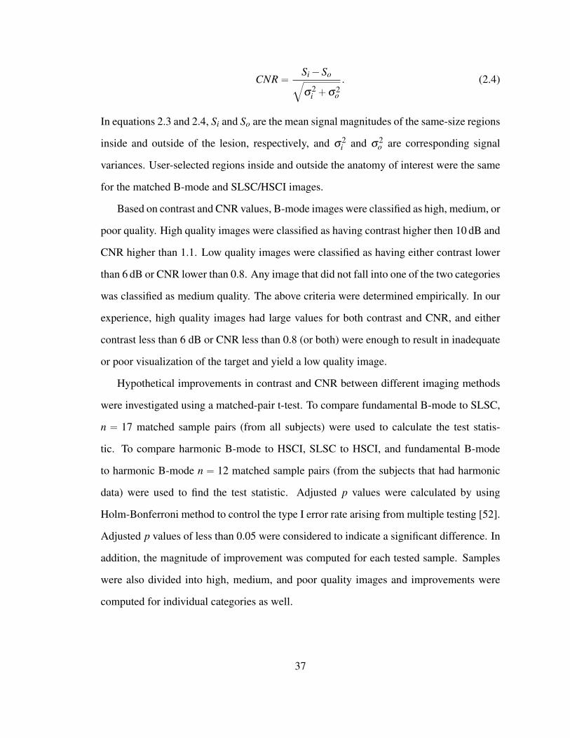
CNR“Si´So
b
σ2i `σ2
o
. (2.4)
In equations 2.3 and 2.4, Si and So are the mean signal magnitudes of the same-size regions
inside and outside of the lesion, respectively, and σ2i and σ2
o are corresponding signal
variances. User-selected regions inside and outside the anatomy of interest were the same
for the matched B-mode and SLSC/HSCI images.
Based on contrast and CNR values, B-mode images were classified as high, medium, or
poor quality. High quality images were classified as having contrast higher then 10 dB and
CNR higher than 1.1. Low quality images were classified as having either contrast lower
than 6 dB or CNR lower than 0.8. Any image that did not fall into one of the two categories
was classified as medium quality. The above criteria were determined empirically. In our
experience, high quality images had large values for both contrast and CNR, and either
contrast less than 6 dB or CNR less than 0.8 (or both) were enough to result in inadequate
or poor visualization of the target and yield a low quality image.
Hypothetical improvements in contrast and CNR between different imaging methods
were investigated using a matched-pair t-test. To compare fundamental B-mode to SLSC,
n “ 17 matched sample pairs (from all subjects) were used to calculate the test statis-
tic. To compare harmonic B-mode to HSCI, SLSC to HSCI, and fundamental B-mode
to harmonic B-mode n “ 12 matched sample pairs (from the subjects that had harmonic
data) were used to find the test statistic. Adjusted p values were calculated by using
Holm-Bonferroni method to control the type I error rate arising from multiple testing [52].
Adjusted p values of less than 0.05 were considered to indicate a significant difference. In
addition, the magnitude of improvement was computed for each tested sample. Samples
were also divided into high, medium, and poor quality images and improvements were
computed for individual categories as well.
37

2.3 Results
Examples of matched B-mode and SLSC/HSCI images are presented in Figures 2.1
through 2.4. Because a limited amount of individual channel data can be saved to create
an SLSC/HSCI image (due to programability limitations of the ultrasound scanner), the
SLSC/HSCI images cover a narrower field of view than the B-mode images. For display
purposes, the SLSC/HSCI images are overlayed on the corresponding B-mode images
between the arrows. B-mode images are displayed on a decibel scale while a linear gray-
scale colormap is used to display SLSC/HSCI images. The dynamic range of the B-mode
images were chosen to optimally visualize structures of interest while the background
brightness of the SLSC and HSCI images were scaled to match that of the B-mode images.
The regions used to calculate the contrast and CNR are indicated by white contour lines in
the B-mode images (the same regions are used in the matched SLSC/HSCI images).
Figure 2.1 demonstrates a high quality fundamental B-mode image (left) and its corre-
sponding SLSC image (right). A large blood vessel appears at the center of field of view
in both images. In the B-mode image, the lumen of the vessel contains low-level acoustic
noise. In the SLSC image, the clutter in the lumen is reduced and the surrounding tissue
is smoother, which results in slightly higher contrast and CNR; 13.5 dB contrast and 1.86
CNR obtained for the SLSC image compared to 11.3 dB contrast and 1.4 CNR obtained
for the B-mode image.
An example of a medium quality fundamental B-mode and its corresponding SLSC
image is shown in Figure 2.2. A blood vessel spanning the depth of the image at the
center of field of view can be seen in both images, with the SLSC image demonstrating
significant improvements in target visualization. Contrast and CNR values were calculated
to be 8.9 dB and 2.05 for SLSC imaging, respectively, and 7.8 dB and 0.95 for B-mode
imaging. Matched harmonic B-mode and HSCI images of the same structure in Figure 2.2
are shown in Figure 2.3. Following the criteria (for contrast and CNR) outlined in section
38

Azimuth (cm)
Depth
(cm
)
B−mode
−8 −4 0 4 8
5
10
15
Azimuth (cm)
B−mode with overlayed SLSC
−8 −4 0 4 8
5
10
15
FIGURE 2.1: High quality fundamental B-mode image (left) and its matched SLSC image (right). Note thatthe SLSC image is the sector inserted into the B-mode image between the arrows. SLSC reduces clutterinside of blood vessels and increases smoothness of the surrounding tissue. The contrast of the large bloodvessel located at the center of field of view at 10 cm depth is 11.3 dB and 13.5 dB, and the CNR is 1.4 and1.86 for B-mode and SLSC images, respectively. The white contour lines in the B-mode image indicate theregions used to calculate contrast and CNR values.
2.2.3, the harmonic B-mode image is classified as medium quality. The overall level of
noise in the image is reduced when compared to the fundamental B-mode (Figure 2.2).
In the HSCI image, clutter is reduced further than in the harmonic B-mode. The CNR
was found to be 2.13 for the HSCI image and 1.16 for B-mode. Contrast is comparable
between the two images; 9 dB for HSCI and 9.6 dB for B-mode.
Figure 2.4 shows a poor quality fundamental B-mode and its matched SLSC image.
Here, the B-mode image has diminished diagnostic value as part of the blood vessel in the
center of field of view is not visible. In the SLSC image, acoustic noise is suppressed and
the structure is clearly visualized. This is reflected in tremendous improvement in contrast
and CNR from B-mode to SLSC. Contrast was found to be 4.44 dB for SLSC compared to
0.26 dB for B-mode imaging. CNR was estimated to be 0.79 for SLSC imaging compared
to 0.03 for B-mode imaging.
39
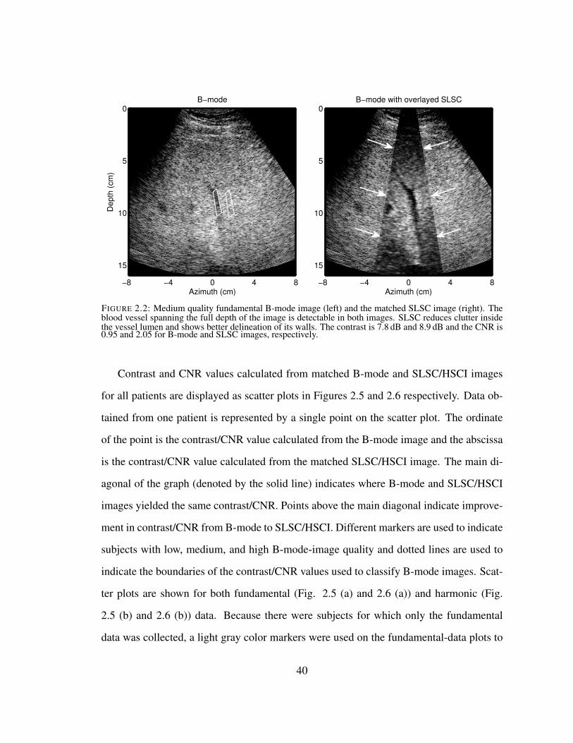
Azimuth (cm)
Depth
(cm
)
B−mode
−8 −4 0 4 8
0
5
10
15
Azimuth (cm)
B−mode with overlayed SLSC
−8 −4 0 4 8
0
5
10
15
FIGURE 2.2: Medium quality fundamental B-mode image (left) and the matched SLSC image (right). Theblood vessel spanning the full depth of the image is detectable in both images. SLSC reduces clutter insidethe vessel lumen and shows better delineation of its walls. The contrast is 7.8 dB and 8.9 dB and the CNR is0.95 and 2.05 for B-mode and SLSC images, respectively.
Contrast and CNR values calculated from matched B-mode and SLSC/HSCI images
for all patients are displayed as scatter plots in Figures 2.5 and 2.6 respectively. Data ob-
tained from one patient is represented by a single point on the scatter plot. The ordinate
of the point is the contrast/CNR value calculated from the B-mode image and the abscissa
is the contrast/CNR value calculated from the matched SLSC/HSCI image. The main di-
agonal of the graph (denoted by the solid line) indicates where B-mode and SLSC/HSCI
images yielded the same contrast/CNR. Points above the main diagonal indicate improve-
ment in contrast/CNR from B-mode to SLSC/HSCI. Different markers are used to indicate
subjects with low, medium, and high B-mode-image quality and dotted lines are used to
indicate the boundaries of the contrast/CNR values used to classify B-mode images. Scat-
ter plots are shown for both fundamental (Fig. 2.5 (a) and 2.6 (a)) and harmonic (Fig.
2.5 (b) and 2.6 (b)) data. Because there were subjects for which only the fundamental
data was collected, a light gray color markers were used on the fundamental-data plots to
40

Azimuth (cm)
Depth
(cm
)B−mode harmonic
−8 −4 0 4 8
0
5
10
15
Azimuth (cm)
B−mode harmonic with overlayed HSCI
−8 −4 0 4 8
0
5
10
15
FIGURE 2.3: Harmonic B-mode image (left) and matched HSCI image (right) of the same vessel as in Figure2.2. Even though the B-mode image is of medium quality, the HSCI image shows notable improvement intarget visualization. The contrast is 9.6 dB and 9 dB and the CNR is 1.16 and 2.13 for B-mode and SLSCimages, respectively.
Azimuth (cm)
Depth
(cm
)
B−mode
−8 −4 0 4 8
4
8
12
Azimuth (cm)
B−mode with overlayed SLSC
−8 −4 0 4 8
4
8
12
FIGURE 2.4: Poor quality fundamental B-mode image (left) and matched SLSC image (right). Noise hascorrupted the B-mode image and does not indicate the presence of a vessel at the center of the field of view.In the SLSC image, the vessel is easily visualized. The contrast is 0.26 dB and 4.44 dB and the CNR is 0.03and 0.79 for B-mode and SLSC images, respectively.
41
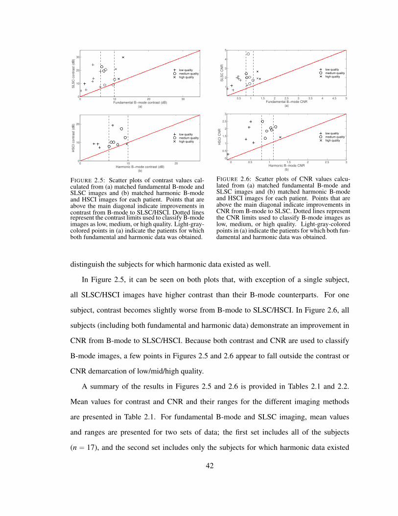
0 10 20 300
10
20
30
Fundamental B−mode contrast (dB)(a)
SL
SC
co
ntr
ast
(dB
)
low quality
medium quality
high quality
0 10 200
10
20
Harmonic B−mode contrast (dB)(b)
HS
CI
co
ntr
ast
(dB
)
low quality
medium quality
high quality
FIGURE 2.5: Scatter plots of contrast values cal-culated from (a) matched fundamental B-mode andSLSC images and (b) matched harmonic B-modeand HSCI images for each patient. Points that areabove the main diagonal indicate improvements incontrast from B-mode to SLSC/HSCI. Dotted linesrepresent the contrast limits used to classify B-modeimages as low, medium, or high quality. Light-gray-colored points in (a) indicate the patients for whichboth fundamental and harmonic data was obtained.
0.5 1 1.5 2 2.5 3 3.5 4 4.5 5
1
2
3
4
5
Fundamental B−mode CNR(a)
SLS
C C
NR
low quality
medium quality
high quality
0 0.5 1 1.5 2 2.5 3
0
0.5
1
1.5
2
2.5
3
Harmonic B−mode CNR(b)
HS
CI C
NR
low quality
medium quality
high quality
FIGURE 2.6: Scatter plots of CNR values calcu-lated from (a) matched fundamental B-mode andSLSC images and (b) matched harmonic B-modeand HSCI images for each patient. Points that areabove the main diagonal indicate improvements inCNR from B-mode to SLSC. Dotted lines representthe CNR limits used to classify B-mode images aslow, medium, or high quality. Light-gray-coloredpoints in (a) indicate the patients for which both fun-damental and harmonic data was obtained.
distinguish the subjects for which harmonic data existed as well.
In Figure 2.5, it can be seen on both plots that, with exception of a single subject,
all SLSC/HSCI images have higher contrast than their B-mode counterparts. For one
subject, contrast becomes slightly worse from B-mode to SLSC/HSCI. In Figure 2.6, all
subjects (including both fundamental and harmonic data) demonstrate an improvement in
CNR from B-mode to SLSC/HSCI. Because both contrast and CNR are used to classify
B-mode images, a few points in Figures 2.5 and 2.6 appear to fall outside the contrast or
CNR demarcation of low/mid/high quality.
A summary of the results in Figures 2.5 and 2.6 is provided in Tables 2.1 and 2.2.
Mean values for contrast and CNR and their ranges for the different imaging methods
are presented in Table 2.1. For fundamental B-mode and SLSC imaging, mean values
and ranges are presented for two sets of data; the first set includes all of the subjects
(n “ 17), and the second set includes only the subjects for which harmonic data existed
42

Table 2.1: Mean and range for contrast and CNR values of hypoechoic/anechoic targets.
Fundamental B-mode SLSC Harmonic B-mode HSCI
Contrast ( dB) mean 5.58 12.36 — —
n“ 17 range 0.26 - 12.52 4.44 - 29.81 — —
Contrast ( dB) mean 5.14 11.08 5.76 9.18
n“ 12 range 0.26 - 10.37 4.44 - 24.15 0.57 - 9.72 1.50 - 19.33
CNR mean 0.75 1.88 — —
n“ 17 range 0.03 - 1.39 0.66 - 4.56 — —
CNR mean 0.69 1.82 0.76 1.70
n“ 12 range 0.03 - 1.28 0.66 - 4.56 0.08 - 1.28 0.28 - 2.50
Table 2.2: Average improvements achieved between fundamental B-mode and SLSC and between harmonicB-mode and HSCI.
Fundamental B-mode to Harmonic B-mode to
B-mode quality SLSC HSCI
Contrast
High 22% 3.4%
Medium 39% 22%
Poor 288% 137%
Overall153% 68%
pă 0.0001, n“ 17 pă 0.01, n“ 12
CNR
High 63% 10%
Medium 158% 102%
Poor 533% 300%
Overall318% 177%
pă 0.0001, n“ 17 pă 0.001, n“ 12
as well (n“ 12). For harmonic B-mode and HSCI, mean values and ranges are shown for
all subjects that had harmonic data (n “ 12). Overall, for both contrast and CNR, SLSC
obtains the highest mean values followed by HSCI, harmonic B-mode, and fundamental
B-mode. Also, all of the mean values obtained for fundamental B-mode and SLSC on
the subset of data (n “ 12) are slightly lower than those obtained on the full set of data
(n“ 17) (Table 2.1).
43

A more detailed comparison is presented in Table 2.2 which shows average improve-
ments (expressed as percentages) of contrast and CNR achiveved between different imag-
ing methods. For each pair of imaging methods, separate improvements for images of
high, medium, and poor quaity are shown in addition to the overall improvement. Due
to the insufficient number of samples for some of the categories, statistical significance
is shown only for the overall improvements (shown are adjusted p values and number of
sample pairs, n, used to calculate the test statistic). Overall, SLSC and HSCI show sig-
nificant improvements in target detection when compared to fundamental and harmonic
B-mode, respectively; adjusted p values are smaller than 0.001 for both contrast and CNR.
In addition, the results obtained from the individual image-quality categories suggest that
the improvements increase as the image quality decreases with the highest percentage
improvements (between fundamental B-mode and SLSC and between harmonic B-mode
and HSCI) observed for poor quality B-mode images. Also, greater improvements are
observed between fundamental B-mode and SLSC than between harmonic B-mode and
HSCI. The improvements between fundamental B-mode and harmonic B-mode and be-
tween HSCI and SLSC are statistically insignificant (adjusted p values are larger than
0.05 for both contrast and CNR). As such, these improvements are not reported in Table
2.2.
2.4 Discussion
SLSC and HSCI tend to reduce clutter and improve the overall image quality compared
to B-mode liver images. As seen in the sample images (Figures 2.1 - 2.4), the most signif-
icant improvements are achieved in visualization of small-size, negative intrinsic-contrast
structures such as blood vessels. While the source of contrast in B-mode images is the
difference in echo brightness, the contrast in SLSC/HSCI images arises from the differ-
ence in signal coherence [24, 66]. This means that in B-mode images, incoherent signals
44

inside of a vessel lumen appear similar to surrounding tissue while in SLSC/HSCI images,
these signals are highly suppressed. As a result, when compared to their matched B-mode
images SLSC/HSCI images display crisper vessel boundaries and reduced clutter inside
of a vessel lumen.
The surrounding tissue appears smoother and more uniform in SLSC/HSCI images
compared to their matched B-mode images (Figures 2.1 - 2.4). We hypothesize that these
differences arise because the mechanisms responsible for speckle noise in SLSC/HSCI
images are different than those in B-mode images. The grainy texture of B-mode im-
ages is due to variations of the speckle brightness, resulting from the constructive and
destructive interference of reflections from sub-wavelength particles. The variance of the
speckle brightness increases with average echo magnitude often reaching large values
[116]. Speckle noise in the SLSC/HSCI images is due to variations of the spatial co-
herence function, which does not depend on echo magnitude and exhibits relatively high
uniformity at low lags [117].
Improvements in target visualization between fundamental B-mode images and SLSC
images and between harmonic B-mode images and HSCI images are supported by sta-
tistically significant differences in target contrast and CNR. For both contrast and CNR,
greater relative improvements are observed between fundamental B-mode and SLSC than
between harmonic B-mode and HSCI. We hypothesize that this is due to the fact that har-
monic B-mode already reduces near-field reverberation clutter, thus leaving HSCI with
less incoherent signal to suppress.
Similarly, an increase in relative contrast/CNR improvements (between B-mode and
SLSC/HSCI) is observed with the decrease in B-mode image-quality (Table 2.2) because
lower quality B-mode images have a stronger incoherent component, meaning that the rel-
ative improvements made by SLSC/HSCI would be higher. As hypothesized, the largest
improvements are seen for the poor quality B-mode images. Some B-mode image-quality
categories lack the number of samples to show statistical significance of these improve-
45

ments. Therefore, hypothesis testing was done only for the overall improvements.
As previously stated, the results did not show significant differences (in contrast or
CNR) between SLSC and HSCI and between fundamental B-mode and harmonic B-mode
images. A power analysis indicated that these tests lacked power due to insufficient num-
ber of samples. As the primary focus of our study was to determine if SLSC and HSCI
produced higher quality images than the delay-and-sum beamforming methods currently
used in clinic and for that purpose, our sample size was sufficiently large.
This study faces several limitations. First, for all study participants, we were unable
to acquire any images of focal lesions in the liver. We are aware of the importance of
lesion detection/visualization in ultrasound liver imaging and acknowledge that this spe-
cific population needs to be included in order to assess the performance of SLSC/HSCI
in fulfilling this task. Second, we are unable to create B-mode images that have similar
high-quality displays as commercial, state-of-art US scanners because access to the so-
phisticated post-processing filters developed by major scanner manufacturers is not readily
available. In addition, the lack of hardware/computational power that would allow faster
acquisition and on-site processing of large amounts of individual-channel data prevented
us from obtaining real-time feedback of SLSC/HSCI images. These issues could be allevi-
ated with new software-based-beamforming platforms that would allow quick acquisition
and access to large amounts of single-channel data. Nevertheless, the results presented
here are encouraging because the improvements in blood vessel visualization demonstrate
that SLSC/HSCI could be well suited for in vivo detection of other anechoic/hypoechoic
targets in the liver (such as focal lesions).
2.5 Conclusion
A study was performed that showed SLSC and HSCI imaging produce higher quality
in vivo liver images than conventional delay-and-sum beamforming methods. SLSC and
46

HSCI images of the livers of 17 randomly selected patients display improved visibility of
blood vessels (i. e. sharper delineation of vessel walls and suppressed clutter in the ves-
sel lumen) as well as higher uniformity of the surrounding tissue when compared to their
matched B-mode images. These observations are supported by statistically significant
improvements in target contrast and CNR from fundamental B-mode to SLSC and from
harmonic B-mode to HSCI. In addition, the magnitude of the improvements obtained by
spatial-coherence imaging increases as the quality of B-mode images decreases; the high-
est relative improvements are observed for poor quality fundamental B-mode images. In
the future, we plan to acquire real-time SLSC/HSCI images by using a computationally
powerful, software-based beamforming system. We also anticipate further exploration of
clinical applications of SLSC/HSCI imaging by recruiting additional patients and conduct-
ing other task-specific studies.
47

3
Short-lag Spatial Coherence Imaging on MatrixArrays: Phantom and In Vivo Validation
3.1 Introduction
High-speed volumetric ultrasound has a unique ability to provide real-time and non-
invasive visualization of anatomy and pathology in three dimensions [29]. However, there
are challenges associated with the small element size of typical 2-D arrays and the use
of broad transmit beams that can lead to suboptimal image quality and decreased diag-
nostic utility of the modality. In particular, small 2-D array elements have relatively high
impedance (compared to 1-D array elements) making them more susceptible to parasitic
capacitance [41, 79, 102, 107]. The small element size also limits the area over which an
element can receive the signal compromising that element’s sensitivity to weak echoes in
a noisy in vivo environment. System sensitivity is further reduced due to the use of broad
transmit beams needed to achieve real-time frame rates [100].
In [54], we extended the use of a recently developed beamforming method, short-
lag spatial coherence (SLSC) imaging [66], to volumetric data in an attempt to improve
image quality in clinical 3-D ultrasound. In particular, we presented a theoretical model
48

for applying SLSC imaging to 2-D arrays as well as simulations showing that volumetric
SLSC imaging improves lesion detectability compared to conventional 3-D delay-and-sum
imaging [54]. Here, we demonstrate the feasibility of volumetric SLSC imaging in vivo
on a modified commercial 3-D ultrasound system.
System architecture of most clinical ultrasound scanners makes implementation of ad-
vanced beamforming methods difficult. These systems provide limited programmability
of transmit waveforms and lack access to the channel echo data. In addition, for the high
element-count 2-D arrays for modern 3-D ultrasound systems, partial beamforming of
the subaperture data is implemented in the handle of the array in order to limit losses in
sensitivity (due to impedance mismatching or parasitic capacitance), as well as to reduce
cable weights and system cost [79]. The resultant inability to access radio-frequency (RF)
data for each element limits the realization of many techniques requiring custom trans-
mit sequences or advanced aperture-domain signal processing, including phase aberration
correction and adaptive beamforming. Such methods have seen limited or no usage on
commercial real-time 3-D systems and are difficult to evaluate in off-line studies without
access to individual channel data.
Noteworthy are several implementations of phase-aberration correction algorithms on
clinical 3-D ultrasound scanners using single channel data of partially beamformed sub-
apertures [55, 56, 57, 75]. Ivancevich et al. [55] implemented multi-lag least-squares
cross-correlation and speckle brightness algorithms and compared their performance in
correcting for physical aberrators using a single sparsely-sampled 2-D array. For the
speckle-brightness method, no off-line processing was used; the entire method was im-
plemented using the scanner beamforming routines. Lindsey et al. [75] implemented a
least-squares cross-correlation method on a pitch-catch setup in order to correct for phase
aberration in 3-D transcranial ultrasound in vivo. Here, each matrix array was used as a
correction source for the opposing array thus allowing estimation of multiple arrival time
maps and reducing the error in aberration correction.
49

Hyun et al. explored the performance of the SLSC method on simulated volumetric
data and showed that for small 2-D subapertures, partial beamforming within subapertures
does not degrade the SLSC-image quality [54]. In the following, we demonstrate the con-
cept of volumetric SLSC imaging using phantom and in vivo liver data from a commercial
matrix array and 3-D ultrasound scanner. Utilizing the system’s large-scale parallel re-
ceive processing, we collected partially-beamformed channel data from the fully-sampled
matrix array at high speeds and reconstructed matched B-mode and SLSC volumes of a
vessel phantom and liver vasculature off-line. Contrast and CNR are computed for the
vessels of interest using complete matched volumes to compare target visibility between
the two beamforming methods. Concurrently acquired 3-D Doppler data is used as a gold
standard for visualizing vasculature in three dimensions.
3.2 Methods
3.2.1 Short-Lag Spatial Coherence Imaging on Matrix Arrays
The spatial coherence of a backscattered ultrasonic wave is a measure of how similar
the echo is at any two points in space. It can be predicted by the Van Cittert-Zernike (VCZ)
theorem as the Fourier transform of the square of transmit beam amplitude if the imaging
target is diffuse scatterers [81]. Spatial coherence can be expressed as spatial correlation
and further simplified to a product of two triangle functions when the diffuse scatterers are
insonified with a narrowband pulse from an unapodized rectangular aperture. The spatial
correlation for this case (of diffuse scatterers) has been derived in [54], and is presented
here for convenience:
RDSp∆x,∆yq “ˆ
1´ˇ
ˇ
ˇ
ˇ
∆xDx
ˇ
ˇ
ˇ
ˇ
˙ˆ
1´ˇ
ˇ
ˇ
ˇ
∆yDy
ˇ
ˇ
ˇ
ˇ
˙
, (3.1)
In 3.1, ∆x and ∆y denote the distance between two points in the aperture plane, and Dx
and Dy denote the transmit aperture size in the x and y dimensions, respectively. The
50

spatial correlation of the pressure field can be estimated from the signals of the individual
elements of a matrix array as
Rpi, jq “
n2ř
n“n1
sipnqs jpnqd
n2ř
n“n1
s2i pnq
n2ř
n“n1
s2jpnq
, (3.2)
where i and j are two elements on the 2-D aperture, sipnq and s jpnq are the signals sampled
by those elements, n is a sample number in the time dimension, and the difference n2´n1
represents the axial kernel length used to calculate interelement correlation and is typically
on the order of a wavelength. Note that the signals sipnq and s jpnq in equation 3.2 are
already delayed to achieve focusing at the desired location.
To create an SLSC volume, first, a region of short lags is defined on the 2-D aperture
to include all element pairs whose signals would have a correlation coefficient above some
value P for the theoretical case of diffuse scatterers. In other words, for every element i, a
set of elements j is defined such that RDSpxi´x j,yi´x jq ě P , 0ă Pă 1. Then, to obtain a
single SLSC voxel, Rpi, jq is computed (by applying equation 3.2 to the individual-element
signals) and summed over all short-lag pairs of i and j. For a complete SLSC volume, the
last step is repeated at each depth for every received individual-element data set [54].
To implement volumetric SLSC imaging on a clinical matrix array, we applied the
above procedure on the partially-beamformed channel data as the signals from the indi-
vidual elements were not accessible.
3.2.2 Rapid Single Channel Acquisition
Single channel data was acquired from a 4z1c matrix array (Siemens Medical Solu-
tions USA, Inc.). This high-element-count 2-D array has both an azimuthal pitch and an
elevational pitch of 0.4 mm. Array elements are grouped in rectangular subapertures that
are beamformed in the handle of the transducer giving signals for 192 system channels. In
51

our previous implementations [26], each channel corresponded to a single array element.
Herein, data from an individual channel refers to data beamformed within a rectangular
subaperture. The array was connected to a modified Siemens Acuson SC2000 scanner
(Siemens Medical Solutions USA, Inc., Mountain View, CA) that has a 64:1 parallel-
receive capability; i.e. it can use the channel data from one transmit event to create up to
64 receive beams in parallel.
The complex data of the individual channels were collected using a full-synthetic re-
ceive sequence, similar to the one described by Dahl et al [26]. With this method, the
full aperture is used for transmit, while the signal from a subset of individual channels is
collected on receive. The same transmit event is repeatedly fired until the signals for each
of the channels (i.e. beamformed subapertures) are collected. Integrating this approach
with parallel receive beamforming on the scanner allows for multiple channels to be ac-
quired at one time, thus reducing the number of transmits needed to acquire a complete
channel-data-set.
For the experiments described herein, a 30:1 parallel receive configuration was used to
collect the data for 180 channels (total of six transmit pulses per image line) at 2.5 volumes
per second. 0.4 seconds was required to obtain a complete single channel data set needed
to reconstruct a full (B-mode or SLSC) volume. The complex I/Q data collected for each
channel was sampled at a rate of 2.5 MHz, which was sufficient to obtain high-resolution
ultrasound images.
3.2.3 Flow Phantom Experiment
The individual-channel data needed to reconstruct complete B-mode and SLSC vol-
umes was acquired on an ATS Laboratories model 523A Doppler phantom (ATS Labora-
tories, Bridgeport, CT) with a 4 mm vessel, using the sequences described in the section
3.2.2. The data was acquired using a transmit frequency of 2.5 MHz and a transmit focus of
60 mm. The field of view spanned 38˝ in azimuth and 19.2˝ in elevation and was interro-
52

gated with 330 transmits that were fired sequentially to populate a 22 by 15 transmit-beam
grid. The dense transmit-beam configuration was used to ensure that the spatial sampling
was sufficient to reconstruct high-resolution B-mode and SLSC volumes.
A water-based corn-starch solution (10 g/l) was constantly flowing through the vessel
while the phantom was scanned, and the conventional 3-D color Doppler volume was
acquired concurrently with the individual channel data to be used as a gold standard for
visualizing the vessel lumen. Because a default Doppler sequence was used on the scanner,
the Doppler data was collected over a different field of view than the channel data. The
Doppler field of view spanned 32˝ in azimuth and 26˝ in elevation and was sampled with
90 Doppler lines using a transmit frequency of 2.5 MHz. Doppler data was processed by
the scanner before acquisition.
3.2.4 In Vivo Experiments
Individual-channel data was also collected in vivo on the liver vasculature of four hu-
man volunteers, ages 29 to 58. Written consent was obtained from all participants, and
the study protocol was approved by the local Institutional Review Board. The same data
acquisition sequences and imaging configuration were used as for the flow-phantom ex-
periment (section 3.2.3). Conventional 3-D color Doppler was used for guidance and
targeting of blood vessels. Color Doppler volumes were acquired concurrently with the
single-channel-acquisition sequence as a gold standard for visualizing the vasculature in
the region of interest (ROI).
3.2.5 Data processing
From the single-channel data, matched B-mode and SLSC volumes were reconstructed
off-line. SLSC volumes were reconstructed following the procedure outlined in section
3.2.1 (for a more detailed description of the reconstruction methods reader is referred to
the Methods section of [54]). Contrast and CNR values were computed for the vessels of
53

interest for complete matched volumes according to the equations 2.3 and 2.4, respectively.
For the sake of clarity, both equations are reproduced bellow:
Contrast “´20log10
ˆ
Si
So
˙
,
CNR“Si´So
b
σ2i `σ2
o
.
Si and So are the mean signal magnitudes of the regions inside and outside of the vessel,
respectively, and σ2i and σ2
o are corresponding signal variances. The regions outside of
the vessels were selected to have the same average speckle brightness as the vessel walls.
The regions inside of the vessels were selected using a Doppler mask. To create the mask,
a general region containing the vessel of interest in the Doppler volume was manually
selected. The dynamic range of the Doppler signal within that region was then limited
to remove the noise and obtain a clean and continuous mask of the vessel lumen. To
minimize the spillage of Doppler signal (mask) outside of the vessel lumen, the cutoff
value for amplitude was calibrated on the vessel-phantom with the known vessel diameter.
The mask was then applied to the matched B-mode and SLSC volumes.
3.3 Results
Examples of 2-D and 3-D images generated from matched B-mode, SLSC, and color-
Doppler volumes are presented in Figures 3.1 through 3.6. The B-mode images are dis-
played on the decibel scale with the dynamic range that allows for the clearest view of the
vessels of interest for a given acquisition. The SLSC images are displayed using a linear
color-map with a dynamic range that has been scaled to match the background brightness
of the B-mode images. The Doppler images are also displayed using a linear map but with
the dynamic range and transparency adjusted (independently of the B-mode and SLSC
images) to show clear and continuous Doppler signal from the vessels of interest. The red
54

contour lines in the 3-D Doppler images highlight the regions of the vessel lumen used to
calculate contrast and CNR for the B-mode and SLSC volumes.
Figure 3.1 shows matched B-mode, SLSC, and color-Doppler volumes reconstructed
from a phantom data set. For the 3-D B-mode and SLSC volumes, cutaway views are
displayed (at 48˝ azimuth and 22˝ elevation angle) in order to expose a 4 mm vessel
that spans the azimuth dimension of the volumes. Orthogonal slices of the volumes in
Figure 3.1 are shown in Figure 3.2 and are selected to optimally display different cross-
sections of the vessel. The vessel can be observed in all 2-D and 3-D images. The SLSC
images demonstrate reduced acoustic noise inside the vessel lumen when compared to
the corresponding B-mode images. The SLSC images also display reduced background
brightness in the upper part of the field of view, which can be attributed to suppression
of reverberant clutter in that region.1 Reverberant clutter appeared as parts of the aperture
were not in full contact with the phantom due to the shape of the phantom and the scanning
geometry employed to obtain optimal Doppler signal. The Doppler images show the vessel
lumen fully populated by color-Doppler signal and the lumen boundaries can be clearly
visualized. Using Doppler signal to select a 3-D region inside the blood vessel, the contrast
and CNR values are calculated to be 2.27 dB and 0.34 for the B-mode volume, and 4.73 dB
and 1.58 for the SLSC volume.
Examples of matching B-mode, SLSC, and color-Doppler images of in vivo liver vas-
culature are shown in Figures 3.3 through 3.6. 2-D and 3-D images are created from two
volumetric data-sets, both acquired from a 29 year old male volunteer, in the same general
region of the liver, but at slightly different angles to demonstrate spatial stability of volu-
metric SLSC imaging. In order to make the vasculature fully visible in the 3-D B-mode
and SLSC images, Figures 3.3 and 3.5 display cutaway views of the volume.
1 We previously showed [66] that the coherence curves for diffuse targets exhibit lower values in thepresence of acoustic noise resulting in darker SLSC pixels/voxels. This is in contrast to B-mode imageswhere average speckle brightness is proportional to signal variance [116] and the regions of diffuse scattererscan appear bright in the presence of clutter.
55

FIGURE 3.1: Left to right: B-mode, SLSC, and color-Doppler 3-D images generated from a phantom. TheB-mode and SLSC images show only a part of the acquired field of view in order to expose a 4 mm vesselspanning the elevation dimension of the volumes. The SLSC image demonstrates improved visualization ofthe vessel cross-section compared to the matched B-mode image. The Doppler image confirms the extent ofthe vessel and shows clear and continuous color-Doppler signal at the location of the vessel lumen.
Azimuth (cm)
Depth
(cm
)
B−mode
−3 0 3
4
8
Azimuth (cm)
SLSC
−3 0 3
4
8
Azimuth (cm)
Doppler
−3 0 3
4
8
Elevation (cm)
Depth
(cm
)
−2 0 2
4
8
Elevation (cm)−2 0 2
4
8
Elevation (cm)−2 0 2
4
8
FIGURE 3.2: Orthogonal slices created from the volumes shown in Figure 3.1. Left to right: matchedB-mode, SLSC, and color-Doppler slices in azimuth plane (top row) and elevation plane (bottom row).The SLSC slices display less clutter inside the vessel lumen and better delineation of the vessel walls thanthe corresponding B-mode slices. In the Doppler slices, the boundaries of the vessel lumen are clearlyvisualized.
56
3-D and 2-D images created from the first in vivo acquisition are presented in Figures
3.3 and 3.4, respectively. In both the B-mode and SLSC volumes of Figure 3.3, a narrow
vessel spanning 6 to 9 cm depth is observed as well as a large vessel in the lower part of
the field of view. In the B-mode volume, the lumen of these vessels contains low level
acoustic noise. In the SLSC volume, clutter inside the large vessel is suppressed and the
surrounding tissue appears smoother. Part of the narrow vessel in the SLSC volume also
shows reduced clutter, but the upper region of the vessel lumen is difficult to distinguish
from the surrounding tissue; this is probably because of the 3-D rendering which makes
the far wall of the vessel appear like clutter. 2-D SLSC slices in Figure 3.4 indeed show
that the clutter in this part of the vessel vessel is suppressed. Using the Doppler signal to
define the region inside of the narrow vessel, the contrast is calculated to be 15.32 dB and
10 dB, and the CNR is calculated to be 1.6 and 2.3 for the B-mode and SLSC volumes,
respectively. The signal from the large vessel has not been captured in the Doppler volume
as the clinical system used to collect the data was designed primarily for cardiac applica-
tion and had difficulties detecting slower hepatic flow. The SLSC volume also shows two
potential small blood vessels (denoted by black arrows) that do not appear in the B-mode
and Doppler volumes. These structures can be more clearly visualized in the azimuth
SLSC slice in Figure 3.4.
Figure 3.4 shows azimuth and elevation (2-D) slices of the volumes displayed in Figure
3.3. Cross-sections of the same blood vessels that are observed in both B-mode and SLSC
volumes are observed in the B-mode and SLSC slices, with SLSC slices showing reduced
noise inside of the vessels and improved edge definition of the vessel walls. 2-D SLSC
images also display details that are not visible in their B-mode counterparts. As suggested,
two potential small blood vessels are located at about 6 cm depth in the azimuth SLSC scan
and are marked by white arrows for clarity. In the corresponding B-mode image, these
strucutres are not visible due to high acoustic noise. The Doppler scans fail to confirm the
presence of the small vessels but they do show the full extent of the narrow vessel located
57
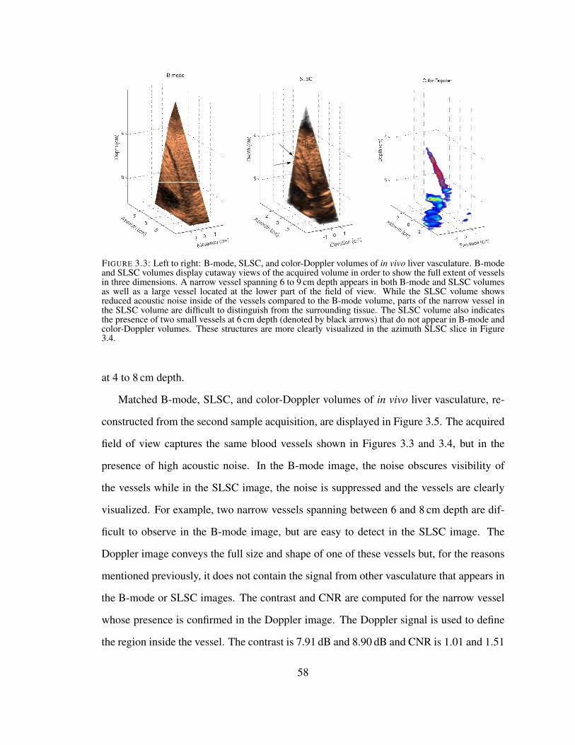
FIGURE 3.3: Left to right: B-mode, SLSC, and color-Doppler volumes of in vivo liver vasculature. B-modeand SLSC volumes display cutaway views of the acquired volume in order to show the full extent of vesselsin three dimensions. A narrow vessel spanning 6 to 9 cm depth appears in both B-mode and SLSC volumesas well as a large vessel located at the lower part of the field of view. While the SLSC volume showsreduced acoustic noise inside of the vessels compared to the B-mode volume, parts of the narrow vessel inthe SLSC volume are difficult to distinguish from the surrounding tissue. The SLSC volume also indicatesthe presence of two small vessels at 6 cm depth (denoted by black arrows) that do not appear in B-mode andcolor-Doppler volumes. These structures are more clearly visualized in the azimuth SLSC slice in Figure3.4.
at 4 to 8 cm depth.
Matched B-mode, SLSC, and color-Doppler volumes of in vivo liver vasculature, re-
constructed from the second sample acquisition, are displayed in Figure 3.5. The acquired
field of view captures the same blood vessels shown in Figures 3.3 and 3.4, but in the
presence of high acoustic noise. In the B-mode image, the noise obscures visibility of
the vessels while in the SLSC image, the noise is suppressed and the vessels are clearly
visualized. For example, two narrow vessels spanning between 6 and 8 cm depth are dif-
ficult to observe in the B-mode image, but are easy to detect in the SLSC image. The
Doppler image conveys the full size and shape of one of these vessels but, for the reasons
mentioned previously, it does not contain the signal from other vasculature that appears in
the B-mode or SLSC images. The contrast and CNR are computed for the narrow vessel
whose presence is confirmed in the Doppler image. The Doppler signal is used to define
the region inside the vessel. The contrast is 7.91 dB and 8.90 dB and CNR is 1.01 and 1.51
58

Azimuth (cm)
Depth
(cm
)
B−mode
−3 0 3
4
8
Azimuth (cm)
SLSC
−3 0 3
4
8
Azimuth (cm)
Doppler
−3 0 3
4
8
Elevation (cm)
Depth
(cm
)
−2 0 2
4
8
Elevation (cm)−2 0 2
4
8
Elevation (cm)−2 0 2
4
8
FIGURE 3.4: 2-D scans created from the volumes shown in Figure 3.3. Left to right: matched B-mode,SLSC, and color Doppler scans in azimuth orientation (top row) and elevation orientation (bottom row).The SLSC images show improved visualization of the vessel cross-sections compared to the correspondingB-mode scans. In partcular, cross-sections of two small vessels can be clearly observed at 6 cm depth in theazimuth SLSC slice (denoted by white arrows); these vessels are not well visualized in the correspondingB-mode image. The Doppler slices fail to confirm the presence of the small vessels but they outline thenarrow vessel located at 4 to 8 cm depth.
for the B-mode and SLSC volumes, respectively.
Azimuth and elevation cross sections of the volumes in Figure 3.5 are shown in Fig-
ure 3.6. Both B-mode scans are of poor quality as the tissue structures are overwritten
by acoustic noise. SLSC scans reduce noise and show improved visualization of the hep-
atic vasculature. Specifically, cross-sections of the narrow vessels located around 6 cm
depth are difficult to detect in the B-mode images but are well observed in their SLSC
counterparts. The presence of one of these vessels is confirmed in the matching Doppler
scans.
Image quality metrics for B-mode and SLSC volumes in Figures 3.2 through 3.6 are
summarized in Table 3.1. In all examples, the SLSC volumes show higher CNR val-
59

FIGURE 3.5: Left to right: B-mode, SLSC, and color-Doppler volumes created from the second in vivodata-set. The 3-D images offer a different view of the same hepatic structures shown in Figures 3.3 and3.4, but contain a significant amount of clutter. The 3-D SLSC image demonstrates reduced clutter andimproved visualization of blood vessels compared to the matched B-mode image. Specifically, two narrowblood vessels spanning 6 to 8 cm depth cannot be visualized in the B-mode image, but the structures areclearly shown in the SLSC image. The shape and size of one of these vessels can also be seen in the 3-DDoppler image.
ues than the matching B-mode volumes. In addition, the B-mode contrast values are
in agreement with of our previous in vivo measurements of clutter magnitude in ane-
choic/hypoechoic regions (which range from about 25 dB to about 5 dB below the mean
brightness of the surrounding tissue) [68].2 For the B-mode volumes created from the
phantom and second in vivo acquisitions, clutter levels are high and the matching SLSC
volumes demonstrate improvements in vessel contrast. For the first in vivo data-set, the B-
mode volume yields higher contrast than the matched SLSC volume with contrast values
being large (clutter being low) for both modalities.
3.4 Discussion
Phantom and in vivo results demonstrate the feasibility of SLSC imaging on a com-
mercial matrix array and 3-D ultrasound scanner. SLSC images of the vessel phantom
(Figures 3.1 and 3.2) convey the extent of the vessel in three dimensions, without sig-
2 In [68], the magnitude of clutter was measured at different points inside of anechoic/hypoechoic regionsin units of dB relative to the mean brightness of the surrounding tissue. Assuming the echogenicity ofblood is significantly lower than the echogenicity of the surrounding tissue, vessel contrast can be used toapproximate mean clutter magnitude inside of the vessel.
60

Azimuth (cm)
Depth
(cm
)
B−mode
−3 0 3
4
8
12
Azimuth (cm)
SLSC
−3 0 3
4
8
12
Azimuth (cm)
Doppler
−3 0 3
4
8
12
Elevation (cm)
Depth
(cm
)
−2 0 2
4
8
12
Elevation (cm)−2 0 2
4
8
12
Elevation (cm)−2 0 2
4
8
12
FIGURE 3.6: Orthogonal slices created from the volumes shown in Figure 3.5. Left to right: matched B-mode, SLSC, and color-Doppler slices in azimuth orientation (top row) and elevation orientation (bottomrow). The azimuth and elevation slices indicate improved visualization of hepatic vasculature achieved byvolumetric SLSC imaging compared to conventional 3-D B-mode. In particular, cross-sections of the narrowblood vessels located around 6 cm depth do not appear in the B-mode images but are clearly visible in theirSLSC counterparts. The presence of one of these vessels is confirmed in the matching Doppler slices.
nificant artifacts, and using the data from a single volumetric acquisition. The in vivo
data-sets (acquired in the same general region of the liver) demonstrate the stability and
consistency of SLSC imaging on a matrix array; the shape and size of the blood vessels
look comparable between the two SLSC volumes despite different scanning orientation
used at each acquisition (Figures 3.3 and 3.5). In all examples, the SLSC volumes are re-
Table 3.1: Image quality metrics for sample phantom and in vivo acquisitions.
AcquisitionPhantom 1st in vivo 2nd in vivo
B-mode SLSC B-mode SLSC B-mode SLSC
Contrast (dB) 2.27 4.73 15.32 10.00 7.91 8.90
CNR 0.34 1.58 1.60 2.30 1.01 1.51
61

constructed from the partially beamformed data. Delaying-and-summing the signals with
subapertures prior to constructing the spatial coherence curves provides averaging of the
channel-noise and ensures that the coherence function is sufficiently sampled in both az-
imuth and elevation dimensions. The improvements in contrast and CNR achieved by this
hybrid SLSC imaging technique are consistent with the results demonstrated from noisy
and noise-free simulations [54].
Sample 2-D and 3-D images reconstructed from the SLSC volumes show improved
visibility of the vessels when compared to their B-mode counterparts (Figures 3.1 - 3.6).
The SLSC imaging on a matrix array integrates the coherence function strictly over the
short-lag region (in both azimuth and elevation dimensions), thus leaving out the incoher-
ent signals present in the long-lag region [54]. Via this mechanism, the SLSC imaging
suppresses incoherent echoes (and thus clutter) inside the vessels that come from the off-
axis scatterers or reverberation, which enhances definition of the vessel walls [24, 66]. In
a B-mode volume, the echo amplitude is displayed instead of coherence, so the incoherent
echoes tend to overwrite and obscure the structures of interest. The rate of acquisition of
single channel data listed in section 3.2.2 and low echogenecity of blood ensure that the
observed improvements in vessel visualization in the SLSC images are not biased by the
motion of blood/corn-starch solution inside of vessel during the acquisition.3
The liver tissue appears smoother and more uniform in the in vivo SLSC images than in
the corresponding B-mode images (Figures 3.3 - 3.6). This smooth texture is not associated
3 Given the data acquisition rates presented in section 3.2.2 the estimated motion of blood/corn-starchsolution during the acquisition of a single imaging line was 0.1 - 0.2 mm, which was unlikely to result ina substantial decorrelation of the echoes from the moving scatterers across the aperture [111]. In addition,due to low echogenecity of blood compared to the surrounding tissue (up to -30 dB [20]), contribution ofthese echoes to the signal received from the vessel lumen is very small compared to the off-axis scatteringand reverberation from the surrounding medium. Any fluctuation in correlation of these weak echoes alonewould therefore not be sufficient to cause a significant change in vessel visualization. Finally, with the singlechannel acquisition sequence described in section 3.2.2 data is collected on 30 channels simultaneously,which means that for majority of channels comprising the region of short lags there is no decorrelation ofsignal due to flow. The last statement would hold true even for the cases of high flow and high echogenecityof scatterers inside of vessel.
62

with the loss of resolution (or information in the image) but it is rather due to reduction in
variance of SLSC pixels.4 We have demonstrated that the variance of the speckle bright-
ness in the SLSC images is lower (than in the corresponding B-mode images) because the
spatial-coherence function exhibits high uniformity (and thus low variance) in the region
of short lags [117]. In addition, the hybrid SLSC imaging technique implemented on the
clinical matrix array averages noise within the subapertures of the array (prior to comput-
ing the coherence curves), which further reduces the variance of SLSC speckle. As shown
in simulation [54], subaperture averaging can effectively reduce speckle noise in the SLSC
images even for small subaperture sizes.
Improvements in vessel visualization between B-mode and SLSC images are supported
by contrast and CNR values computed for the complete B-mode and SLSC volumes (Table
3.1). Observed CNR values are in agreement with the simulation results in [54]. For
example, the plots in Figure 10 (in [54]) show that CNR of a -12 dB lesion in the presence
of low and medium acoustic noise (up to element SNR of -20 dB) is between 2.8 and
3.0 for the SLSC volumes formed using 8 x 8 element subapertures; CNR values for the
corresponding B-mode volumes are about 1.5. These values are comparable to CNR values
obtained for the B-mode and SLSC volumes from the first in vivo acquisition (1.6 and 2.3,
respectively). Further, CNR values obtained from the second in vivo acquisition (1.01
and 1.51 for the B-mode and SLSC volumes, respectively) are within the range of values
shown in plots in Figure 10 (in [54]), at high noise levels. In particular, at -20 dB element
SNR, simulations predict CNR of a -12 dB lesion to be about 1.0 for B-mode and about
1.8 for hybrid SLSC imaging (implemented on 8 x 8 element subapertures).
The analysis presented in this chapter faces several limitations. First, the data was
collected using a phased matrix array which was designed primarily for cardiac imaging
and had a relatively small aperture. With this setup, we were unable to create B-mode
4 Our previous measurements of resolution in the SLSC images (defined as width of a point target ordistance between two point targets), indicate that it is highly dependent on the level of noise and that it isnot directly related to the texture size.
63
images that had high-resolution displays similar to those obtained with large linear arrays
that are typically used in abdominal imaging. Second, the Doppler confirmation is lack-
ing for some vessels in the in vivo acquisitions because the cardiac system used to collect
the Doppler data was not calibrated to capture slower hepatic flow and acquisitions were
not synchronized with the cardiac cycle (the latter causing significant discontinuities in
the Doppler signal in the presence of pulsatile flow). Because contrast and CNR could be
only computed for those vessels that were detected with Doppler, a more quantitative com-
parison between the corresponding B-mode and SLSC volumes could not be performed.
Finally, visualizing the differences between the complete B-mode and SLSC volumes is
limited due to the lack of an efficient way to display volumetric data. Nevertheless, the
results indicate that the hybrid SLSC imaging technique as implemented on the clinical
matrix array improves visualization of blood vessels in three-dimensions and they encour-
age its use for imaging other structures.
3.5 Conclusion
We have successfully demonstrated the concept of volumetric SLSC imaging on the
clinical 3-D ultrasound scanner and matrix array. Through a series of phantom and in
vivo liver experiments, we showed that 3-D and 2-D images generated from the SLSC
volumes exhibit improved visualization of the vessels compared to their matched B-mode
images. We used the color Doppler signal to confirm the presence of the vessels of interest
and to define the 3-D regions used in contrast and CNR calculations. SLSC volumes
yielded higher CNR values than the matched B-mode volumes while the contrast values
were comparable between the two modalities. Our finding also showed that delaying-and-
summing the signals with subapertures (of the 2-D array) prior to constructing the spatial
coherence curves did not compromise the quality of SLSC images; this is in agreement
with our previous simulation results. In the future, we hope to expand our single-channel-
64

acquisition tool to matrix arrays with larger apertures that are more suitable to abdominal
imaging but also further improve data acquisition rates which would allow us to extend
volumetric SLSC imaging to cardiac application.
65
4
Blocked Elements Signal Characteristics andImpact on Visualizing Anechoic and Hypoechoic
Targets
4.1 Introduction
When imaging with ultrasound through the chest wall, it is not uncommon for parts
of the array to be positioned against the ribs, preventing them from properly transmitting
and/or receiving acoustic pulses [51]. Other structures such as scar tissue or air in the
lungs can also introduce a high acoustic impedance mismatch and effectively block ar-
ray elements, or parts of them, during an ultrasound scan [49, 121]. Blocked elements
tend to significantly degrade overall image quality, limit the acoustic window, and impede
visualization of the structures of interest [70]. With the development of large-aperture,
high-element-count, 2-D arrays and their potential use in transthoracic imaging, detecting
and compensating for the blocked elements is becoming increasingly important. In the
remainder of Chapter 4, we focus on the ways to detect blocked elements and to measure
their impact on visibility of anechoic targets in vivo.
The system architecture of most clinical ultrasound scanners makes it difficult to as-
66

sess the problem of blocked elements in vivo. Typically, the raw echoes from individual
elements can be collected from a clinical system only through custom pulse sequencing,
which is difficult to realize in real-time due to limits on the internal memory size and
data-transfer rates. In addition, in most high-element count 2-D arrays, signals from the
individual elements are partially beamformed in the handle of the transducer [79], and
are not accessible even through the custom sequencing; this prevents complete and precise
characterization of blocked parts of the array. To our knowledge, there have been no in vivo
attempts to characterize signals from blocked elements and to measure image-degradation
they introduce.
There have been several ex vivo studies aimed at understanding the mechanisms and
extent of image degradation in transthoracic ultrasound. Notably, Hinkelman et al. [51]
measured arrival-time and energy-level fluctuations across a mechanically scanned 2-D
aperture for ultrasonic wavefronts that propagated through the extracted samples of human
chest-wall. The average rms values were 21.3 ns and 1.57 dB for arrival-time and energy-
level fluctuations, respectively. The receive 2-D apertures were windowed to minimize
parts blocked by bone and to isolate distortions introduced by soft-tissue inhomogeneities;
the above-reported results are thus clinically relevant only for intercostal imaging with
small arrays.
As a part of their transcostal, high-intensity, focused ultrasound (HIFU) feasibility
study, Aubry et al. measured distortions of the ultrasound beam transmitted through the
ribs [3]. In simulation and ex vivo experiments, they found that waves that propagated
through bone had a pressure amplitude about six times lower than waves that propagated
through soft tissue (in between the ribs). Compared to the control transmit beampatterns
measured in the absence of acoustic obstacles, the beampatterns associated with trans-
rib imaging experienced a mean spreading in the mainlobe half-width of 1.25 mm and
an increase in the sidelobe levels of up to 20 dB. However, the transducer used in the ex
vivo study was designed for HIFU experiments (transmitting at 1 MHz with 200 elements,
67
8 mm in diameter each) leaving it unclear to what extent the beam would be distorted in a
conventional imaging setup.
In [62], Khokhlova et al. presented a more systematic analysis of intensity distributions
at the focal plane of a HIFU transducer during transrib therapy. In particular, they assessed
the appearance of secondary foci due to periodic structure of the ribs, the phenomenon
known as focus splitting. They simulated propagation from a phased array containing
254 randomly distributed elements (7 mm in diameter each), and predicted that ribs can
lead to the appearance of anywhere between one and five focal maxima, depending on the
ratio of sizes of intercostal spaces and ribs. The diameter of each focus is similar to the
diameter of the focal spot in the absence of ribs. In addition, the absolute intensities
in the focal plane are a function of position of ribs relative to the transducer surface;
maximum focus amplitude is achieved when the beam area covered by ribs is minimal.
These conclusions were reached using diffraction theory and pursuing both analytic and
numerical approaches. In all cases, a strong agreement was achieved between the two
solutions, and with the intensity measurements from the ex vivo setup. The studies in [62]
and [3] were both aimed at ultrasound therapy, and did not address the effect of beam
degradation (due to blocked elements) on visibility of distributed and anechoic targets.
In this chapter, we characterize the signals on blocked elements and measure their
impact on visualizing anechoic/hypoechoic targets using simulated, phantom, and in vivo
data from fully sampled 2-D apertures. Utilizing the full-wave simulation tool and a com-
mercial 3-D ultrasound system, we demonstrate methods for detecting blocked elements
based on the amplitude and cross-correlation of their signals. From simulated and in vivo
data we also reconstruct B-mode images of liver vasculature using receive apertures of
different sizes; vessel contrast and CNR are measured to assess visibility of targets as a
function of number of blocked elements in the aperture. In order to compare performance
of 1-D versus 2-D arrays for transcostal imaging, the contrast/CNR measurements are ob-
tained for receive apertures growing in one and two dimensions of the array. In Chapter
68
5, we continue to address the problem of blocked elements. In particular, we measure the
loss of focus quality and clutter levels when imaging through the ribs with large synthetic
apertures ex vivo. We then evaluate different beamforming schemes aimed at recovering
this loss of image quality.
4.2 Methods
4.2.1 Full-wave Simulations
We simulated single channel data received on a fully sampled 2-D array while imaging
liver intercostally. We first created a 3-D acoustic map of parts of thorax and abdomen
that would be captured in an intercostal liver scan, and then we used the full-wave code
developed by Pinton et al. [96] to model wave propagation through the medium, including
the effects of non-linearity, attenuation, and multiple scattering (reverberation).
The 3-D acoustic map of tissue was built using the National Library of Medicine’s
Visible Human data set, which provides high resolution registered optical, MRI, and CT
scans of the entire male and female bodies. Following the procedure outlined in [98], each
structure in the region of interest was declared as one of the six tissue types (homoge-
neous, fat, muscle, connective, liver, or bone tissue) and assigned appropriate values for
its acoustic properties (speed of sound, density, nonlinearity, and attenuation). Acoustic
properties of each tissue type were determined from the data compiled by Goss et al. [44,
45] and are listed in Table 4.1. While the reported speed of sound in bone is as high as
3000 m/s, a significantly lower value (800 m/s) was used in the simulation to allow for
more efficient temporal sampling of wave propagation. The bone density was set so that
the acoustic impedance mismatch between bone and soft tissue remained similar as in real
tissue.
In order to simulate speckle generating targets, small local variations in speed of sound
(average variation of 5 % from the surrounding tissue) were introduced throughout the
69
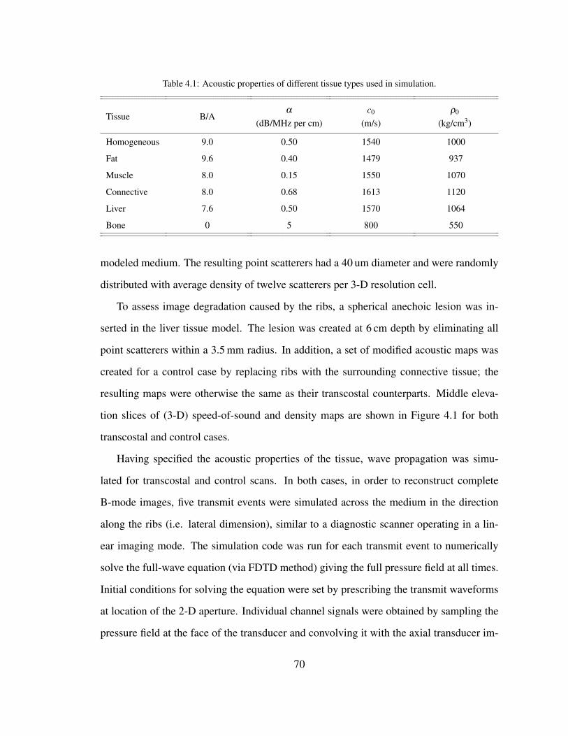
Table 4.1: Acoustic properties of different tissue types used in simulation.
Tissue B/Aα
(dB/MHz per cm)c0
(m/s)ρ0
(kg/cm3)
Homogeneous 9.0 0.50 1540 1000
Fat 9.6 0.40 1479 937
Muscle 8.0 0.15 1550 1070
Connective 8.0 0.68 1613 1120
Liver 7.6 0.50 1570 1064
Bone 0 5 800 550
modeled medium. The resulting point scatterers had a 40 um diameter and were randomly
distributed with average density of twelve scatterers per 3-D resolution cell.
To assess image degradation caused by the ribs, a spherical anechoic lesion was in-
serted in the liver tissue model. The lesion was created at 6 cm depth by eliminating all
point scatterers within a 3.5 mm radius. In addition, a set of modified acoustic maps was
created for a control case by replacing ribs with the surrounding connective tissue; the
resulting maps were otherwise the same as their transcostal counterparts. Middle eleva-
tion slices of (3-D) speed-of-sound and density maps are shown in Figure 4.1 for both
transcostal and control cases.
Having specified the acoustic properties of the tissue, wave propagation was simu-
lated for transcostal and control scans. In both cases, in order to reconstruct complete
B-mode images, five transmit events were simulated across the medium in the direction
along the ribs (i.e. lateral dimension), similar to a diagnostic scanner operating in a lin-
ear imaging mode. The simulation code was run for each transmit event to numerically
solve the full-wave equation (via FDTD method) giving the full pressure field at all times.
Initial conditions for solving the equation were set by prescribing the transmit waveforms
at location of the 2-D aperture. Individual channel signals were obtained by sampling the
pressure field at the face of the transducer and convolving it with the axial transducer im-
70

Transcostal Acquisition Control Acquisition
elevation (cm)
axia
l (c
m)
ρ
−1 0 1
0
1
2
3
4
5
6
7
8
elevation (cm)
axia
l (c
m)
c
−1 0 1
0
1
2
3
4
5
6
7
8
elevation (cm)
axia
l (c
m)
ρ
−1 0 1
0
1
2
3
4
5
6
7
8
elevation (cm)a
xia
l (c
m)
c
−1 0 1
0
1
2
3
4
5
6
7
8
FIGURE 4.1: Speed of sound and density maps used for the transcostal simulations (left) and for the controlsimulations (right). For the transcostal case, a rib can be observed at about 1 cm depth in the left side of fieldof view in both maps. The acoustic maps used for the control simulations are identical to their transcostalcounterparts except ribs are replaced by the connective tissue. In both speed-of-sound maps, the lesionboundaries are denoted using a black dashed line.
pulse response. Specifically, the center frequency of transmitted waves was set at 2.5 MHz
and the transducer impulse response was set to yield a fractional bandwidth of 0.5. The
2-D aperture extended 1.9 cm in lateral and 1.4 cm in elevation dimension, and was posi-
tioned so that roughly one half of it was blocked by ribs during the transcostal scan. The
individual channel signals from each transmit event were used to beamform 50 receive
lines to ensure sufficient sampling in the lateral dimensions.
4.2.2 Phantom Experiments
Using the sequences described in section 3.2.2, the individual-channel data needed
to reconstruct complete B-mode volumes was acquired on a tissue mimicking phantom
(CIRS, Norfolk, VA). A region of diffuse scatterers in the phantom was first imaged
71

through a piece of absorbing rubber that was placed directly underneath the array to block
a part of the 2-D aperture. The absorbing rubber was then removed and the same region of
phantom was imaged to collect a control data set. The data was acquired using a transmit
frequency of 2.5 MHz and a transmit focus set at 60 mm. A relatively dense transmit-beam
configuration was used to ensure the field-of-view (FOV) was sampled at the Nyquist fre-
quency at the focal depth. Specifically, 330 transmits were fired sequentially to populate a
22 by 15 transmit-beam grid that spanned 38˝ in azimuth and 19.2˝ in elevation dimension.
4.2.3 In Vivo Study
Using the same sequences and imaging configuration as in 4.2.2, the individual-channel
data was acquired on the liver vasculature of five human volunteers, ages 29 to 59. Written
consent was obtained from all participants, and the study protocol was approved by the lo-
cal Institutional Review Board. Livers were first imaged intercostally, so that parts of the
2-D aperture were blocked by the ribs. To obtain the control data (with all the transducer
elements free to transmit and receive pulses), the same vasculature was also imaged sub-
costally, away from the ribs. In both cases, the probe was angled so that the vasculature of
interest was in the middle of the FOV. To minimize the motion artifacts, the patients were
asked to hold their breath and to remain still for the duration of each acquisition.
4.2.4 Data Processing and Receive Aperture Growth
For simulated, phantom, and in vivo data sets, the amplitude and the nearest-neighbors
normalized cross-correlation of the individual channel signals were computed to detect
blocked elements. The two quantities were averaged axially, over a 4 cm range centered
around the transmit focus, and observed as functions of channel position on the receive 2-D
aperture. Channels/elements were classified as blocked if their depth-averaged amplitude
was -8 dB or lower (compared to the maximum channel amplitude on the 2-D aperture),
and if their nearest-neighbor normalized cross-correlation was less than 0.5. The above
72
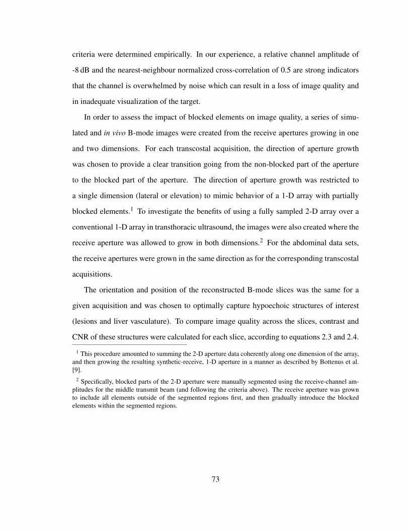
criteria were determined empirically. In our experience, a relative channel amplitude of
-8 dB and the nearest-neighbour normalized cross-correlation of 0.5 are strong indicators
that the channel is overwhelmed by noise which can result in a loss of image quality and
in inadequate visualization of the target.
In order to assess the impact of blocked elements on image quality, a series of simu-
lated and in vivo B-mode images were created from the receive apertures growing in one
and two dimensions. For each transcostal acquisition, the direction of aperture growth
was chosen to provide a clear transition going from the non-blocked part of the aperture
to the blocked part of the aperture. The direction of aperture growth was restricted to
a single dimension (lateral or elevation) to mimic behavior of a 1-D array with partially
blocked elements.1 To investigate the benefits of using a fully sampled 2-D array over a
conventional 1-D array in transthoracic ultrasound, the images were also created where the
receive aperture was allowed to grow in both dimensions.2 For the abdominal data sets,
the receive apertures were grown in the same direction as for the corresponding transcostal
acquisitions.
The orientation and position of the reconstructed B-mode slices was the same for a
given acquisition and was chosen to optimally capture hypoechoic structures of interest
(lesions and liver vasculature). To compare image quality across the slices, contrast and
CNR of these structures were calculated for each slice, according to equations 2.3 and 2.4.
1 This procedure amounted to summing the 2-D aperture data coherently along one dimension of the array,and then growing the resulting synthetic-receive, 1-D aperture in a manner as described by Bottenus et al.[9].
2 Specifically, blocked parts of the 2-D aperture were manually segmented using the receive-channel am-plitudes for the middle transmit beam (and following the criteria above). The receive aperture was grownto include all elements outside of the segmented regions first, and then gradually introduce the blockedelements within the segmented regions.
73

4.3 Results
4.3.1 Individual Channel Signals
The amplitude and the nearest-neighbour normalized cross-correlation of the channel
signals collected on the lesion phantom are shown in Figures 4.2 and 4.3, for the control
acquisition and for the acquisition through a layer of sound-absorbing rubber, respectively.
The two quantities are displayed through depth for each row of receive channels in a series
of images (a through l) starting with the upper most row of channels in image a. For
every image, the axial range is limited to 4 cm around the Tx focus, where the nearest-
neighbour cross-correlation values are expected to follow the Van-Cittert-Zernike theorem.
The channel amplitude is normalized and displayed on the decibel scale with the dynamic
range that allows for clear distinction between the blocked and non-blocked parts of the
aperture. Normalized cross-correlation is displayed using a linear map with the dynamic
range from 0 to 1.
For the control acquisition (Figure 4.2), both sets of images look uniform with the nor-
malized cross-correlation values being relatively high (close to one). For the acquisition
where a layer of rubber was blocking the right side of the array (Figure 4.3), a sharp drop
in amplitude/cross-correlation is observed over this part of the aperture.
Examples of images characterizing the individual-channel signals acquired on the liv-
ers of two subjects (out of five) are presented in Figures 4.4 through 4.8. In particular, the
images of channel amplitude and the nearest-neighbour normalized cross-correlation in
Figures 4.4 and 4.5 are created from a transcostal and an abdominal data set, respectively,
both acquired on the liver of a 59-year old male. The two quantities are shown for all
rows of channels over 4 cm depth, in a similar format as in Figures 4.2 and 4.3. For the
abdominal acquisition (Figure 4.4), the images indicate no significant difference between
the individual-channel signals received across the aperture. For the transcostal acquisition
(Figure 4.5), the amplitude and the nearest-neighbour cross-correlation are low for the
74
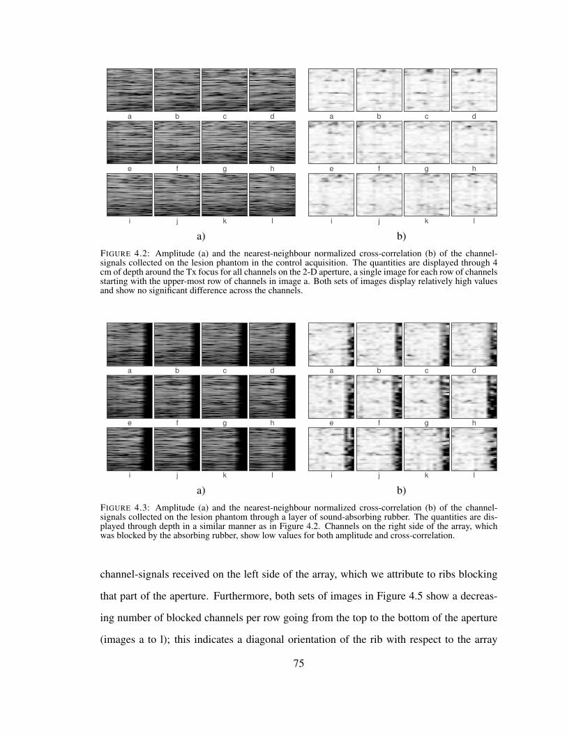
a b c d
e f g h
i j k l
a b c d
e f g h
i j k l
a) b)
FIGURE 4.2: Amplitude (a) and the nearest-neighbour normalized cross-correlation (b) of the channel-signals collected on the lesion phantom in the control acquisition. The quantities are displayed through 4cm of depth around the Tx focus for all channels on the 2-D aperture, a single image for each row of channelsstarting with the upper-most row of channels in image a. Both sets of images display relatively high valuesand show no significant difference across the channels.
a b c d
e f g h
i j k l
a b c d
e f g h
i j k l
a) b)
FIGURE 4.3: Amplitude (a) and the nearest-neighbour normalized cross-correlation (b) of the channel-signals collected on the lesion phantom through a layer of sound-absorbing rubber. The quantities are dis-played through depth in a similar manner as in Figure 4.2. Channels on the right side of the array, whichwas blocked by the absorbing rubber, show low values for both amplitude and cross-correlation.
channel-signals received on the left side of the array, which we attribute to ribs blocking
that part of the aperture. Furthermore, both sets of images in Figure 4.5 show a decreas-
ing number of blocked channels per row going from the top to the bottom of the aperture
(images a to l); this indicates a diagonal orientation of the rib with respect to the array
75

surface. While the images in Figures 4.4 and 4.5 are noisier than their phantom counter-
parts (Figures 4.2 and 4.3),3 the extent of the blocked part of the aperture in the transcostal
acquisition can be still clearly visualized.
Figures 4.6 and 4.7 show the images of channel amplitude and the nearest-neighbour
normalized cross-correlation reconstructed from the second pair of transcostal and abdom-
inal acquisitions, in the presence of high acoustic noise. The images are formatted in the
same way as in Figures 4.2 through 4.5. For the abdominal acquisition (Figure 4.6), al-
though corrupt by noise, signals do not appear significantly different across the channels.
A bright horizontal band at about 7 cm depth can be attributed to a piece of connective tis-
sue or to a blood vessel boundary. For the transcostal acquisition (Figure 4.7), the images
h through l show lower amplitude and cross-correlation values (than the other images in
the figure), which suggests that those rows of channels are partially blocked by bone. Due
to high levels of clutter, it is difficult to identify the individual blocked channels by visual
inspection of images h through l.
The channel amplitude and the nearest-neighbour normalized cross-correlation dis-
played in Figures 4.6 and 4.7 are averaged through depth and are shown over the extent of
the 2-D aperture in Figure 4.8, for both abdominal and transcostal data sets. Both quan-
tities are displayed using a linear grayscale colormap, with the dynamic range from 0 to
1. For the abdominal acquisition (Figure 4.8 a)), the average amplitude and the nearest-
neighbour cross-correlation exhibit high uniformity over the entire surface of the array.
For the transcostal acquisition (Figure 4.8 b)), a region of dark pixels located in the lower-
right corner of both images clearly shows the extent of the blocked part of the aperture and
indicates a diagonal orientation of the rib. Signals received on this part of the array have
8.4 dB lower average amplitude than the signals received on the remainder of elements.
The average amplitude and the average nearest-neighbour cross-correlation of the sim-
3 In particular, the decorrelation among the neighbouring channels in Figures 4.4 and 4.5 is attributed to invivo clutter.
76

a b c d
e f g h
i j k l
a b c d
e f g h
i j k l
a) b)
FIGURE 4.4: Amplitude (a) and the nearest-neighbour normalized cross-correlation (b) of the channel-signals collected on the liver of the first subject during an abdominal scan. The quantities are displayedas functions of depth in a similar manner as in Figures 4.2 and 4.3. Both sets of images display relativelyhigh values and show no significant difference across the channels. Noise in the nearest-neighbour cross-correlation images is attributed to in vivo clutter.
a b c d
e f g h
i j k l
a b c d
e f g h
i j k l
a) b)
FIGURE 4.5: Amplitude (a) and the nearest-neighbour normalized cross-correlation (b) of the channel-signals collected on the liver of the first subject transcostally. The quantities are displayed through a rangeof depths around the Tx focus in a similar manner as in Figures 4.2 through 4.4. The amplitude and cross-correlation are low for the channel-signals received on the left side of the array due to ribs blocking that partof the aperture. Going from image a to l, the number of blocked channels in a row decreases suggestingdiagonal orientation of the rib with respect to the array surface. Despite the presence of acoustic noise,boundaries of the blocked part of the aperture are clearly observed.
ulated channel signals are shown in Figure 4.9. The receive-channel signals are char-
acterized for the middle Tx beam of a simulated transcostal scan, and for the matching
77

a b c d
e f g h
i j k l
a b c d
e f g h
i j k l
a) b)
FIGURE 4.6: Amplitude (a) and the nearest-neighbour normalized cross-correlation (b) of the channel-signals acquired on the liver of the second subject during an abdominal scan. Both quantities are displayedin a similar format as in Figures 4.2 through 4.5. In both sets of images, no significant difference can beobserved across the channels. A bright band in the lower part of images is due to a piece of connective tissue,or to a blood vessel boundary.
a b c d
e f g h
i j k l
a b c d
e f g h
i j k l
a) b)
FIGURE 4.7: Amplitude (a) and the nearest-neighbour normalized cross-correlation (b) of the channel-signals collected on the liver of the second subject, transcostally. The quantities are displayed in a similarmanner as in Figures 4.2 through 4.6. The images h through l show lower amplitude and cross-correlationvalues relative to other images in the figure, which indicates that a part of the array is blocked by a rib.However, due to presence of high acoustic noise, it is difficult to identify the individual blocked channels byvisual inspection.
simulation where the ribs are substituted by the surrounding connective tissue (i.e. no-rib
scan). The amplitude and the nearest-neighbour cross-correlation are averaged over 4 cm
of depth around the Tx focus, and are displayed across the receive 2-D aperture using
78
Lateral element
Ele
vation e
lem
ent
Amplitude
12 24 36
1
18
36
Lateral element
ρ
12 24 36
Lateral element
Ele
vation e
lem
ent
Amplitude
12 24 36
1
18
36
Lateral element
ρ
12 24 36
a) b)
FIGURE 4.8: Average amplitude (left) and average nearest-neighbour normalized cross-correlation (right)of the channel-signals collected off the 2-D array during an abdominal (a) and a transcostal (b) liver scans.The images are created by averaging through depth the channel amplitude and cross-correlation displayedin Figures 4.6 and 4.7. For the abdominal acquisition, both quantities appear relatively uniform throughoutthe extent of the aperture indicating echoes have been received without significant obstruction. For thetranscostal acquisition, a region of low values in the bottom right corner (of both images) is attributed to arib blocking that part of the aperture. Shape of the blocked region suggests diagonal orientation of the ribwith respect to the array surface.
a linear grayscale map and the dynamic range from 0 to 1. For the no-rib scan (Figure
4.9 a)), both quantities are uniform across the array. For the (simulated) transcostal scan
(Figure 4.9 b)), the top four rows of channels (that are positioned above the rib in Fig-
ure 4.1) display lower amplitude and cross-correlation values than the rest of the aperture.
While there is an agreement between the amplitude and cross-correlation images for both
simulations, the cross-correlation image created from the transcostal scan displays sharper
boundaries of the blocked region (of the aperture) than its corresponding amplitude image.
4.3.2 Growing Aperture B-mode Images
Examples of B-mode images of liver reconstructed from the simulated control (i.e.
no-rib4) and transcostal acquisitions are shown in Figures 4.10 and 4.11, respectively. In
both Figures, going from left to right images are created using the receive apertures that in-
crease in size along the elevation dimension of the array and comprise the upper 33, 67, and
100 % of the total physical aperture. For the transcostal simulation, this implies that the
receive aperture grows to include the blocked elements first, and the non-blocked elements
4 The terms ’no-rib’ and ’control’ are used interchangebaly in this section to reffer to the simulation casein which the acoustic properties of bone were substituted with those of the surrounding connective tissue.
79
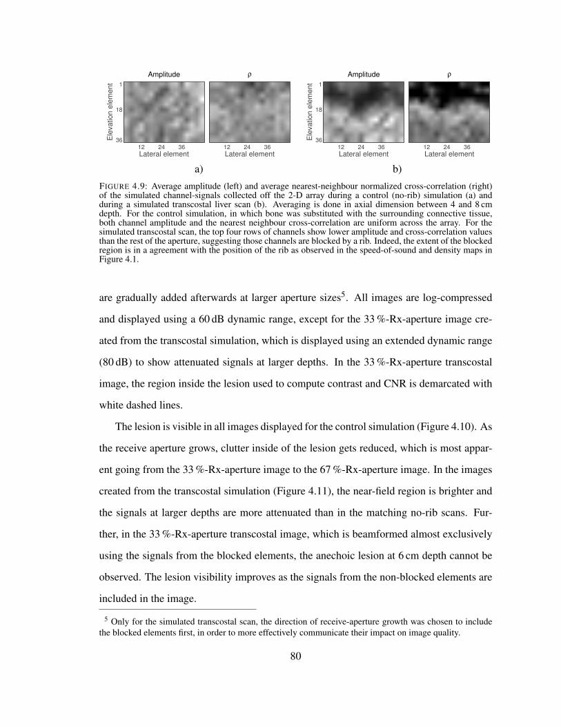
Lateral element
Ele
va
tio
n e
lem
en
t
Amplitude
12 24 36
1
18
36
Lateral element
ρ
12 24 36
Lateral element
Ele
va
tio
n e
lem
en
t
Amplitude
12 24 36
1
18
36
Lateral element
ρ
12 24 36
a) b)
FIGURE 4.9: Average amplitude (left) and average nearest-neighbour normalized cross-correlation (right)of the simulated channel-signals collected off the 2-D array during a control (no-rib) simulation (a) andduring a simulated transcostal liver scan (b). Averaging is done in axial dimension between 4 and 8 cmdepth. For the control simulation, in which bone was substituted with the surrounding connective tissue,both channel amplitude and the nearest neighbour cross-correlation are uniform across the array. For thesimulated transcostal scan, the top four rows of channels show lower amplitude and cross-correlation valuesthan the rest of the aperture, suggesting those channels are blocked by a rib. Indeed, the extent of the blockedregion is in a agreement with the position of the rib as observed in the speed-of-sound and density maps inFigure 4.1.
are gradually added afterwards at larger aperture sizes5. All images are log-compressed
and displayed using a 60 dB dynamic range, except for the 33 %-Rx-aperture image cre-
ated from the transcostal simulation, which is displayed using an extended dynamic range
(80 dB) to show attenuated signals at larger depths. In the 33 %-Rx-aperture transcostal
image, the region inside the lesion used to compute contrast and CNR is demarcated with
white dashed lines.
The lesion is visible in all images displayed for the control simulation (Figure 4.10). As
the receive aperture grows, clutter inside of the lesion gets reduced, which is most appar-
ent going from the 33 %-Rx-aperture image to the 67 %-Rx-aperture image. In the images
created from the transcostal simulation (Figure 4.11), the near-field region is brighter and
the signals at larger depths are more attenuated than in the matching no-rib scans. Fur-
ther, in the 33 %-Rx-aperture transcostal image, which is beamformed almost exclusively
using the signals from the blocked elements, the anechoic lesion at 6 cm depth cannot be
observed. The lesion visibility improves as the signals from the non-blocked elements are
included in the image.
5 Only for the simulated transcostal scan, the direction of receive-aperture growth was chosen to includethe blocked elements first, in order to more effectively communicate their impact on image quality.
80

Contrast and CNR of the anechoic lesions observed in Figures 4.10 and 4.11 are plotted
as functions of receive-aperture size in Figure 4.12. The two image-quality metrics are
presented on the same graph using the dual-axis plots with contrast values displayed on
the left y-axis and CNR values displayed on the right y-axis. Colored solid and dashed
lines are used to plot the image-quality metrics for the transcostal and control simulations,
respectively. The aperture size is expressed as a percentage of total number of receive
elements in the array used for image reconstruction. Vertical black dashed lines indicate
sizes of the receive apertures used to reconstruct images in Figures 4.10 and 4.11.
For the control simulation, both contrast and CNR increase gradually as the receive
aperture grows. For the transcostal simulation, the image quality metrics stay low as the
images are beamformed using only blocked elements. Specifically, as the Rx aperture
grows to include 33 % of total array size, contrast and CNR for the transcostal simulation
increase from 2.14 dB to 3.1 dB, and from 0.34 to 0.49, respectively. Following the same
change in the Rx aperture for the no-rib simulations, lesion contrast and CNR increase
from 9.36 dB to 14 dB, and from 1.19 to 1.49, respectively. Lesion contrast and CNR
(computed for the transcostal simulation) start to improve as the non-blocked elements are
added to the Rx aperture, reaching maxima of 14.8 dB and 1.42 at the full Rx aperture.
Sample B-mode images of in vivo liver vasculature reconstructed using receive aper-
tures of different sizes are shown in Figures 4.13 and 4.14. The images are created from
the same abdominal and transcostal acquisitions used to generate Figure 4.8 with the re-
ceive apertures growing in the elevation dimension. Going from left to right the images in
each figure are beamformed using the upper 8, 67, and 100 % of receive array-elements.
The means that for the transcostal scan, the receive aperture is started with the non-blocked
elements only, and the blocked elements are added gradually at larger aperture sizes. All
images are displayed on a decibel scale with the dynamic range chosen to optimally visu-
alize vasculature of interest for a given acquisition.
Figure 4.13 shows the selected growing-aperture images created from the abdominal
81
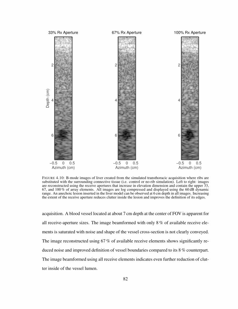
Azimuth (cm)
Depth
(cm
)
33% Rx Aperture
−0.5 0 0.5
2
4
6
Azimuth (cm)
67% Rx Aperture
−0.5 0 0.5
2
4
6
Azimuth (cm)
100% Rx Aperture
−0.5 0 0.5
2
4
6
FIGURE 4.10: B-mode images of liver created from the simulated transthoracic acquisition where ribs aresubstituted with the surrounding connective tissue (i.e. control or no-rib simulation). Left to right: imagesare reconstructed using the receive apertures that increase in elevation dimension and contain the upper 33,67, and 100 % of array elements. All images are log compressed and displayed using the 60 dB dynamicrange. An anechoic lesion inserted in the liver model can be observed at 6 cm depth in all images. Increasingthe extent of the receive aperture reduces clutter inside the lesion and improves the definition of its edges.
acquisition. A blood vessel located at about 7 cm depth at the center of FOV is apparent for
all receive-aperture sizes. The image beamformed with only 8 % of available receive ele-
ments is saturated with noise and shape of the vessel cross-section is not clearly conveyed.
The image reconstructed using 67 % of available receive elements shows significantly re-
duced noise and improved definition of vessel boundaries compared to its 8 % counterpart.
The image beamformed using all receive elements indicates even further reduction of clut-
ter inside of the vessel lumen.
82
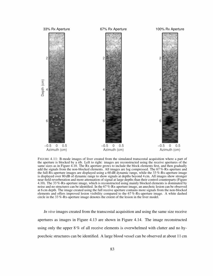
Azimuth (cm)
67% Rx Aperture
−0.5 0 0.5
2
4
6
Azimuth (cm)
100% Rx Aperture
−0.5 0 0.5
2
4
6
Azimuth (cm)
Depth
(cm
)
33% Rx Aperture
−0.5 0 0.5
2
4
6
FIGURE 4.11: B-mode images of liver created from the simulated transcostal acquisition where a part ofthe aperture is blocked by a rib. Left to right: images are reconstructed using the receive apertures of thesame sizes as in Figure 4.10. The Rx aperture grows to include the block elements first, and then graduallyadd the signals from the non-blocked elements. All images are log compressed. The 67 %-Rx-aperture andthe full-Rx-aperture images are displayed using a 60 dB dynamic range, while the 33 %-Rx-aperture imageis displayed over 80 dB of dynamic range to show signals at depths beyond 4 cm. All images show strongernear-field reverberation and more attenuation of signal at large depths than their control counterparts (Figure4.10). The 33 %-Rx-aperture image, which is reconstructed using mainly blocked elements is dominated bynoise and no structures can be identified. In the 67 %-Rx-aperture image, an anechoic lesion can be observedat 6 cm depth. The image created using the full receive aperture contains more signals from the non-blockedelements and offers improved lesion visibility compared to the 67 %-Rx-aperture image. A white dashedcircle in the 33 %-Rx-aperture image denotes the extent of the lesion in the liver model.
In vivo images created from the transcostal acquisition and using the same size receive
apertures as images in Figure 4.13 are shown in Figure 4.14. The image reconstructed
using only the upper 8 % of all receive elements is overwhelmed with clutter and no hy-
poechoic structures can be identified. A large blood vessel can be observed at about 11 cm
83

25 50 75 1000
5
10
15
20
Co
ntr
ast
(dB
)
Aperture Size (%)
0
0.5
1
1.5
CN
R
0
0.5
1
1.5
CN
R
ContrastCNR
FIGURE 4.12: Contrast and CNR of the anechoic lesions in the liver model measured as functions of thereceive-aperture size during the simulated no-rib scan (dashed lines) and during the simulated transcostalacquisition (solid lines). The two image quality metrics are presented on the same graph using the dual-axisplots with contrast values displayed on the left y-axis and CNR values displayed on the right y-axis. Forthe control simulation, both contrast and CNR increase gradually with the receive aperture size reachingmaxima of 15.9 dB and 1.58, respectively, at full aperture. For the transcostal simulation, the two image-quality metrics remain low as the receive aperture contains mainly blocked elements. Specifically, as the Rxaperture grows to reach 33 % of the total array size, contrast and CNR increase by 1 dB and 0.15, respectively.For the same change in the Rx aperture for the control simulations, contrast and CNR increase by 4.6 dB and0.4, respectively. For the transcostal simulation, as the non-blocked elements are added to the Rx aperture,contrast and CNR grow to reach maxima of 14.8 and 1.42, respectively, at full-aperture. As a reference. thevertical black dashed lines denote the sizes of the Rx-apertures used to reconstruct the displayed B-modeimages (in Figures 4.10 and 4.11).
depth at the right side of FOV in the images reconstructed using 67 % and 100 % of the
available receive aperture with the 67 %-receive-aperture image displaying clearer vessel
lumen and more pronounced vessel walls.
Contrast and CNR of the vessels observed in Figures 4.13 and 4.14 are plotted over a
range of receive-aperture sizes in Figure 4.15. The plots are formatted in a similar manner
as in Figure 4.12, with the following modifications. The image quality metrics obtained
for each acquisition are plotted on a separate graph. Contrast and CNR values that corre-
spond to the displayed B-mode images (in Figures 4.13 and 4.14) are additionally denoted
with the colored circles, while the vertical black dashed lines are used to indicate the
aperture size at which contrast and CNR achieve maxima for the transcostal acquisition.
Furthemore, due to diagonal orientation of the rib with respect to the array surface for the
84

transcostal acquisition (Figure 4.14), the receive aperture was also grown along both di-
mensions to potentially offer improved discrimination of the blocked region. Colored solid
and dashed lines are used to plot the image-quality metrics following the receive-aperture
growth in one and two dimensions, respectively.
For the abdominal acquisition (Figure 4.15 left), both contrast and CNR of the vessel
increase as more elements are used to beamform the images reaching maxima of 11.4 dB
and 1.57, respectively, at full aperture. This trend is independent of the direction of receive
aperture growth. For the transcostal acquisition (Figure 4.15 right), the two image-quality
metrics improve as the receive aperture grows until noisy signals from the blocked ele-
ments are introduced. For the receive aperture growing in the elevation dimension (solid
lines), maximum values of contrast and CNR are 10 dB and 1.46, respectively, and are
both measured when (the upper) 66.7 % of available receive aperture is used to beamform
an image. When all receive elements are used in image reconstruction, contrast and CNR
decrease to 9 dB and 1.36, respectively. Image-quality metrics obtained for the transcostal
acquisition and receive-aperture growth in 2-D (dashed lines in the right graph of Figure
4.15) exhibit similar general behavior as their 1-D counterparts except measurements are
noisier and maxima are slightly lower.
Changes in contrast and CNR following the receive-aperture growth in one and two
dimensions are summarized for the abdominal and transcostal acquisitions in all five sub-
jects in Table 4.2.
85

Azimuth (cm)
Depth
(cm
)
8% Rx Aperture
−4 −2 0 2 4
4
8
Azimuth (cm)
67% Rx Aperture
−4 −2 0 2 4
4
8
Azimuth (cm)
100% Rx Aperture
−4 −2 0 2 4
4
8
FIGURE 4.13: B-mode images of in vivo liver vasculature acquired through the abdomen and reconstructedusing receive apertures of different sizes. Left to right: images are reconstructed using the receive aperturesthat increase in elevation dimension and contain the upper 8, 67, and 100 % of array elements. All imagesare log compressed and displayed using the 45 dB dynamic range. A vessel located in the center of FOV atabout 7 cm depth can be observed for all three receive-aperture sizes. Increasing the extent of the receiveaperture reduces clutter and improves visibility of the vessel in the resulting images.
Azimuth (cm)
De
pth
(cm
)
8% Rx Aperture
−4 −2 0 2 4
8
12
Azimuth (cm)
67% Rx Aperture
−4 −2 0 2 4
8
12
Azimuth (cm)
100% Rx Aperture
−4 −2 0 2 4
8
12
FIGURE 4.14: B-mode images of in vivo liver vasculature acquired transcostally and reconstructed using thereceive apertures of the same sizes as in Figure 4.13. The receive aperture is grown to gradually transitionfrom the non-blocked region to the blocked region of the array. All images are log compressed and displayedusing the 45 dB dynamic range. When only 8 % of receive elements are used, the image is overwhelmedwith noise and no structures can be identified. In the 67 % receive-aperture image, a large blood vessel canbe observed in the right side of FOV at about 9 cm depth. The image created using the full receive apertureincludes the noise from the blocked elements and displays higher levels of clutter inside of the vessel lumencompared to its 67 %-receive-aperture counterpart.
86

Abdominal Acquisition Transcostal Acquisition
25 50 75 1000
5
10
15
Co
ntr
ast
(dB
)
Aperture Size (%)
0.5
1
1.5
CN
R
Contrast
CNR
25 50 75 1006
8
10
Co
ntr
ast
(dB
)
Aperture Size (%)
1
1.5
CN
R
Contrast
CNR
FIGURE 4.15: Contrast and CNR as functions of the receive-aperture size for the blood vessels capturedduring the abdominal acquisition (left) and transcostal acquisitions (right). Colored solid and dashed linesare used to plot values for the receive apertures growing along one and two dimensions of the array, respec-tively. Colored circles additionally denote the values that correspond to the displayed B-mode images (inFigures 4.13 and 4.14). For the abdominal acquisition (left), both contrast and CNR increase with receiveaperture size reaching maxima of 11.4 dB and 1.57, respectively, at full aperture. This trend follows both1-D and 2-D aperture growth. For the transcostal acquisition (right), the two image-quality metrics improveas the receive aperture grows until signals from the blocked elements are included in the image. For thereceive aperture growing in the elevation dimension (solid lines), contrast and CNR reach maxima of 10 dBand 1.46, respectively, at the 66.7 % receive-aperture, and then decrease monotonically to 9 dB and 1.36,respectively, at full aperture. As a reference, the receive-aperture size at maximum for the transcostal acqui-sition is denoted by black vertical dashed line in both plots. Contrast and CNR measurements obtained forthe transcostal acquisition and 2-D aperture growth (right side, colored dashed lines) are noisier and achievelower maxima than their 1-D aperture-growth counterparts.
87

Tabl
e4.
2:C
hang
esin
imag
equ
ality
follo
win
gth
ere
ceiv
eap
ertu
regr
owth
inon
ean
dtw
odi
men
sion
sfo
rtr
ansc
osta
lan
dab
dom
inal
acqu
isiti
ons
infiv
edi
ffer
entp
atie
nts.
Patie
nt
num
ber
Cha
nge
inC
ontr
ast(
%)
Cha
nge
inC
NR
(%)
Ape
rtur
ein
crea
se(%
ofR
x
aper
ture
)Tr
ansc
osta
lA
bdom
inal
Tran
scos
tal
Abd
omin
al
1-D
2-D
1-D
2-D
1-D
2-D
1-D
2-D
1-D
2-D
1-3
2.9
\a17
.7\
-21.
88\
20.0
0\
56.2
\
2-1
7.4
-31.
231
.140
.3-3
.37
-6.5
2-2
.89
12.0
050
.055
.6
3-1
5.9
\36
.8\
-6.8
5\
27.6
4\
50.0
\
4-1
8.2
\12
5.3b
\-1
2.50
\10
3.85
b\
66.7
\
5-1
1.7
-22.
457
.473
.7-5
.88
-6.5
737
.74
52.0
850
.074
.4
mea
ns-1
9.2
-24.
135
.742
.1-1
0.10
-10.
8620
.62
27.9
354
.660
.6
std
8.0
7.6
16.5
23.3
7.38
6.66
17.2
817
.32
7.3
9.8
aD
irec
tion
ofap
ertu
regr
owth
was
chos
ento
yiel
dth
ehi
ghes
tpea
k-co
ntra
st/C
NR
valu
esfo
ra
tran
scos
tala
cqui
sitio
n.Fo
rso
me
subj
ects
,an
addi
tiona
lde
gree
offr
eedo
mha
sno
tcha
nged
the
dire
ctio
nof
optim
alap
ertu
regr
owth
resu
lting
inth
esa
me
peak
-con
tras
t/CN
Rva
lues
asfo
rthe
sing
le-d
imen
sion
aper
ture
-gro
wth
.The
sere
peat
edva
lues
are
notd
ispl
ayed
tore
duce
clut
ter.
bL
ack
ofa
good
acou
stic
win
dow
thro
ugh
the
abdo
men
resu
lted
inlo
wim
age
qual
ityan
dex
trem
ely
larg
ech
ange
sin
cont
rast
and
CN
Rfo
rthi
sacq
uisi
tion.
The
seva
lues
have
been
trea
ted
asou
tlier
san
dha
veno
tbee
nin
clud
edin
mea
n/st
anda
rdde
viat
ion
calc
ulat
ions
.
88

4.4 Discussion
4.4.1 Detection of Blocked Elements
Simulation, phantom, and in vivo results demonstrate that blocked elements can be
detected based on low amplitude and cross-correlation values of their signals. In particu-
lar, the elements were declared as blocked if their average amplitude was -8 dB or lower
(relative to the maximum channel amplitude in the aperture) and if their average nearest-
neighbour cross-correlation was less than 0.5. The locations of the blocked elements in
the phantom and simulation acquisitions were verified based on the (known) positions of
the acoustic obstacles. Specifically, in the images of channel amplitude and the nearest-
neighbour normalized cross-correlation created from the phantom acquisition through a
piece of sound-absorbing rubber (Figure 4.3), the array elements that were positioned di-
rectly above the rubber (on the right side of the array) show lower values than the rest
of the aperture. In a similar way, in the aperture-domain images created from the simu-
lated transcostal scan (Figure 4.9 a)), parts of the 2-D aperture that were in the geometric
shadow of a rib 6 display lower amplitude and cross-correlation values than the remaining
channels.
The validity of the blocked element-detection method is further confirmed with the
matched control data obtained on phantoms and in simulation. When collecting the matched
control data, the acoustic obstacles were removed from the wave-propagation path while
the rest of imaging conditions remained the same as in the corresponding blocked-element
acquisitions. For the control acquisition in a tissue-mimicking phantom, this meant that the
region of diffuse scatterers was imaged without the sound-absorbing rubber in the prop-
agation path. For the control simulations, the acoustic maps of the thorax were modified
by replacing bone with the surrounding connective tissue. For both acquisitions, the re-
sulting images of channel amplitude and the nearest neighbour cross-correlation (Figures
6 The acoustic shadow cast by ribs in the simulated transcostal scan can be predicted from the speed-of-sound and density maps in Figure 4.1.
89

4.2 and 4.9 a) are uniform and display high values across the channels, which confirms
the absence of acoustic obstacles. This indicates that the blocked elements detected in
the matching transcostal simulations/phantom experiments can be attributed only to the
presence of acoustic obstacles.
The channel amplitude and cross-correlation images reconstructed from the in vivo
acquisitions support the results obtained from the simulation and phantom experiments.
The images of average channel amplitude and average nearest-neighbour cross-correlation
reconstructed from an abdominal liver scan (Figure 4.8 a)) display uniformity across the
channels in the absence of an acoustic obstacle. In the corresponding images created from
the matching transcostal acquisition, a region of low values can be observed in the bottom
right corner (Figure 4.8 b)), and is attributed to a rib blocking that part of the aperture.
The examples of aperture-domain images reconstructed from the in vivo scans also
demonstrate that depth averaging improves blocked-element detection in the presence of
high acoustic noise. The in vivo images that display channel amplitude and the nearest-
neighbour cross-correlation as functions of depth (Figures 4.4 through 4.7) are noisier than
their phantom counterparts (Figures 4.2 and 4.3). Noise in the channel data is attributed to
the in vivo clutter and can especially affect the nearest-neighbour cross-correlation images.
We have shown previously that in the presence of clutter, spatial covariance can decrease
even at low lag values [66]. As the cross correlation takes on lower values, its estimates
exhibit significantly higher variance according to the VCZ theorem [117]. The amplitude
and cross-correlation images reconstructed from the transcostal acquisition on the second
subject are corrupted with acoustic noise (Figure 4.7), and while low values indicate that
part of the aperture is blocked by a rib, the individual blocked channels cannot be identi-
fied. However, after those images are averaged axially (over 4 cm depth), the extent of the
blocked regions can be clearly visualized in the resulting 2-D aperture images (Figure 4.8
b)).
90

4.4.2 Decreased Visibility of Anechoic and Hypoechoic Targets due to Blocked Elements
Signals received on the blocked channels are overwhelmed with noise and they degrade
visibility of anechoic/hypoechoic targets. The B-mode image created from the transcostal
simulations using the upper 33 % of the receive aperture is saturated with noise and the
anechoic lesion at 6 cm depth is not visible (Figure 4.10). As observed in the correspond-
ing channel amplitude and cross-correlation images (Figure 4.9 b)), the receive aperture
used to create this B-mode is comprised almost entirely of the blocked elements. The
B-mode image created from the matching control simulation with the same-size Rx aper-
ture shows the lesion with a contrast of 9.36 dB and CNR of 1.19 (Figures 4.11 and 4.12).
In addition, the contrast and CNR plots in Figure 4.12 show that the lesion visibility in
the simulated transcostal scans stays low as the Rx aperture is expanded to include more
blocked elements.
The B-mode images reconstructed form the in vivo acquisitions indicate that turning
off blocked elements could improve contrast and CNR of the anechoic/hypoechoic targets.
As observed in the B-mode images created from the transcostal acquisition in Figure 4.14,
when the blocked elements are added to the Rx aperture to increase its size from 66 % to
100 % of the total array size, vessel contrast and CNR decrease from 10 dB to 9 dB, and
from 1.46 to 1.36, respectively. Again, this is contrasted with the matching abdominal
acquisition where the vessel contrast and CNR increase monotonically with the receive
aperture size. Similar trends have been observed in the other four subjects. Adding signals
from the blocked elements results in the mean drop in contrast of up to 24 %, while the
average drop in CNR (computed for the same changes in the receive apertures) is measured
at 10 % (Table 4.2). Excluding signals from the blocked elements in the image could
therefore partially recover loses in vessel contrast and CNR.
The analysis of in vivo and simulated B-mode images presented in this Chapter faces
several limitations. The images reconstructed from the transcostal acquisitions fail to
91

demonstrate that fully sampled 2-D apertures offer improved discrimination of the blocked
regions compared to conventional 1-D arrays. In particular, the 2-D aperture growth yields
larger improvements in contrast and CNR than the 1-D aperture growth only for two sub-
jects (Table 4.2). In contrast and CNR plots created from a sample transcostal acquisition
(Figure 4.15), maximum values achieved for the case of 1-D aperture growth are larger
than maxima for the 2-D aperture growth, despite the diagonal orientation of the rib with
respect to the array surface (Figure 4.8). This can be attributed to the fact that the size
and location of the blocked regions change with the Tx beam direction, and that this kind
of variation makes it difficult to track smaller changes in contrast and CNR. One way to
improve discrimination of blocked regions (in matrix arrays) would be to grow the receive
apertures independently for each transmit beam.
There are several discrepancies between the trends observed in simulated and in vivo B-
mode images. The difference in lesion contrast and CNR between the simulated transcostal
and control images (reconstructed using the full Rx aperture) is not as large as the corre-
sponding difference between the in vivo transcostal and abdominal images. Further, unlike
the in vivo images created from the abdominal acquisitions, the B-mode images created
from the control (no-rib) simulation do not show significant changes in lesion visibility
for the larger receive-aperture sizes. These (unexpected) trends in simulation results can
be paritally attributed to crude tissue models employed. For example, inhomogeneities
in subcutaneous tissue are roughly sampled, and ribs are presented as uniform regions of
bone tissue, while in reality, they have a more layered structure. In addition, contrast and
CNR measurements can vary depending on a particular realization of speckle, and the sim-
ulation measurements ought to be averaged over multiple realizations to allow for a fair
comparison with the in vivo results.
92
5
Blocked Element Compensation Methods asapplied to Large Coherent Apertures
5.1 Introduction
The use of large apertures in medical ultrasound has the potential to improve image
resolution and visibility of anechoic and hypoechoic targets at larger depths. However,
when imaging through the ribs, acoustic obstacles and inhomogeneities can cause dimin-
ishing returns for increasing aperture size. Large apertures are more susceptible to partial
blockage by bone. In addition, wavefront distortions induced by intercostal soft tissues
can make it difficult to preserve signal coherence across large array surfaces. Both mech-
anisms can degrade the quality of transthoracic scans and diminish diagnostic utility of
increased aperture size.
In Chapter 4, we described simulation and in vivo studies where we imaged liver vas-
culature transcostally using a clinical 2-D array. We demonstrated a method to detect ele-
ments blocked by ribs and to measure the resulting loss of vessel contrast and CNR. Here,
we apply blocked-element detection to large synthetic aperture data acquired through rib
samples ex vivo, and we evaluate different beamforming methods aimed at recovering the
93

loss of image quality.
Several methods have been proposed for alleviating beam degradation during high-
intensity, focused ultrasound (HIFU) treatment through the ribs [3, 6, 7, 21]. In time-
reversal mirror (or phase-conjugation1) [3, 7, 21], signals from a point source located at
the focus are recorded, time-reversed, and re-emitted on each element. Alternatively, in-
stead of assigning a range of amplitude and phase values across the transducer surface,
elements located in the geometric shadow of ribs are turned off while the remaining trans-
mit elements are uniformly weighted; this is referred to as a geometric approach in [7].
The time-reversal method accounts for diffraction effects and distributed tissue inhomo-
geneities making it more effective (than geometric approach) at reducing sidelobe levels
at the focal plane and energy deposited on ribs. However, it requires the physical presence
of a point source at the focus, or modeling wave propagation from a point source using CT
or MRI data.
In an ex vivo experiment, Aubry et al. applied the time-reversal mirror to focus the
transmit beam behind a sample of porcine ribs [3]. The correction resulted in a 5 dB de-
crease in sidelobes, while the ratio between the energy delivered at the target location to
the total emitted energy increased six times. As a part of the same study, the geometric
approach was simulated with qualitatively similar results, except the energy-increase at
the target location was 13 % lower than for the time-reversal mirror. Bobkova et al. com-
pared geometric and time-reversal-based compensation methods directly in simulation, for
an idealized radiator [7]. Both approaches yielded approximately a two-fold increase in
intensity at the focus (compared to no-compensation), while the time-reversal resulted in
less energy deposited on the ribs than the geometric approach; power loss on the ribs was
1, 7.5, and 58 % for the time-reversal, geometric compensation, and no-compensation,
respectively. An upgraded version of time-reversal compensation scheme involved de-
1 The time reversal method is applied to the pulsed beams while the phase conjugation method is used forcontinuous wave transmit.
94

composition of a time-reversal operator (DORT method) and was proposed by Cohard et
al. [21].
To improve the efficacy of a transcostal HIFU treatment, Ballard et al. implemented
adaptive refocusing on a dual-mode (imaging plus therapy) array [6]. Complex weights for
the array elements were computed by solving a constrained optimization problem where
the goal was to maximize the intensity at the target location and minimize the intensity
across the ribs. Images obtained with the array were used to infer locations of the ribs and
target. In an ex vivo setup that utilized a Plexiglas ribs phantom, the desired changes in
energy distribution after refocusing were confirmed through the direct temperature mea-
surements and through changes in echogenecity of the images.
An adaptive beamforming method for improving the quality of transthoracic images
was developed by Li et al. [70]. They used the information from multiple receive beams
to estimate locations and amplitudes of acoustic sources and to suppress the undesired
sidelobe contributions. The estimates were obtained via the method of total least squares,
and as such were robust to the imperfections in the model. The approach by Li et al.
was effective in improving phantom images of point-targets and distributed targets but
the additional complexity of bimodal targets prevented its in vivo implementation. In all
experiments, the elements blocked by ribs were labeled as missing and were not used in
image formation.
In Chapter 4, we presented a method to detect blocked elements, and we measured
image degradation they cause while trying to visualize anechoic and hypoechoic targets
in vivo. In the following, we apply the blocked-element detection and compensation to
large synthetic apertures while imaging point targets through canine rib samples ex vivo.
Specifically, large synthetic transmit and receive apertures spanning across multiple ribs
are created by collecting the channel data from a fully sampled clinical matrix array at mul-
tiple and known array locations. To improve image quality, blocked elements are detected
and retroactively turned off, while the apertures covering intercostal spaces are either com-
95

pounded, or coherently summed using uniform and adaptive channel-weighting schemes.
Clutter levels and point spread functions are measured to evaluate the compensation meth-
ods, and to assess the effect of aperture size on image quality. As a reference, some of
the beamforming schemes are also applied to synthetic aperture data collected through a
section of canine abdomen, in the absence of acoustic obstacles. Arrival-time surfaces are
reconstructed for all acquisitions to estimate the tissue-induced aberration, and to offer
further means to understand and compensate for the loss of focus quality in transthoracic
imaging.
5.2 Methods
5.2.1 Large Coherent 2-D Aperture Acquisitions
Large coherent 2-D aperture data sets were created by collecting full synthetic data
from a Siemens 4z1c matrix array (Siemens Medical Solutions USA, Inc.) at multiple
and known array positions. This high-element-count 2-D array has a 1.92 cm-by-1.44 cm
aperture footprint and a pitch of 0.4 mm in both dimensions. Array elements are grouped
in square subapertures that are beamformed in the handle of the transducer giving signals
for 192 system channels. While in the previous work [26] each channel corresponded to
a single array element, herein data from an individual channel refers to data beamformed
within a rectangular subaperture. With the full synthetic sequence, signals are collected for
each transmit/receive pair of channels. The array was connected to a modified Siemens
Acuson SC2000 scanner (Siemens Medical Solutions USA, Inc., Mountain View, CA)
that has a 64:1 parallel-receive capability which was used to increase acquisition rate of
channel signals as described in (Section) [58].
The 4z1c array was positioned using a high-precision motorized translation stage setup
that provided four degrees of freedom. Specifically, the setup consisted of three linear
translation stages arranged orthogonally to one another (2 x Newport UTM100, 1 x Newport
96

ILS100, Newport Corporation, Santa Clara, CA), and of a rotation stage (Newport URS50)
that allowed the transducer to be rotated around its elevation axis. The accuracy of the lin-
ear translation stages was better than 5 um and their unidirectional repeatability was better
than 1.5 um. The rotation stage had a specified accuracy of 0.03˝, unidirectional repeata-
bility of 0.002˝, and could provide a range of motion of 180˝. By adjusting the angle of
rotation around its elevation axis, the transducer could be mechanically steered to image
the same region of interest from different lateral locations. The translation stage assembly
was fixed on a portable cart, on top of a 212x 102x 82fiberglass water tank.
−20−1001020
0
20
40
60
80
lateral (mm)
axia
l (m
m)
−5
0
5
−5 0 5
late
ral (m
m)
elevation (mm)
a) b)
FIGURE 5.1: Transducer locations used to collect large synthetic aperture data (a) and geometry of an indi-vidual 4z1c aperture (b). Dashed lines indicate look-direction at each transducer position; they all intersectat the point-target location (denoted with a red circle). Adjacent apertures overlap by half-of-the-transducerlength. The resulting synthetic aperture is three times longer than an individual 4z1c aperture.
For the experiments described herein, the full synthetic aperture data was collected
97

at five lateral transducer positions spaced half-of-the-transducer length apart. At each
position, the transducer was mechanically steered towards the region of interest. This
ensured that Tx beams fired from individual channels at different array positions achieved
maximum overlap necessary to synthesize high resolution images. Synthetic Tx/Rx data
from different array positions was summed to increase the lateral extent of the physical
aperture (1.92 x 1.44 cm) and generate a large virtual aperture (5.76 x 1.44 cm). The
geometry of the setup employed to collect large synthetic aperture data as well as geometry
of an individual 4z1c aperture are shown in schematics in Figure 5.1.
5.2.2 Ex vivo Experiments
Using sequences and setup described in section 5.2.1, large coherent 2-D aperture data
was acquired on a custom-designed point target phantom. The phantom consisted of a
sapphire sphere 0.2 mm in diameter that was suspended in a slab of gelatin. The phantom
was imaged through freshly excised sections of canine chest wall, and through a section of
canine abdomen. For each acquisition, the tissue samples were placed directly underneath
the array. Both phantom and the tissue were immersed in a tank filled with the (10:1)
mixture of water and n-propanol that had speed of sound of approximately 1540 m/s. 170 g
of salt was added to 19 liters of mixture to make it osmotically neutral and preserve the
internal tissue structure.2 For the transcostal acquisitions, the rib samples were oriented
with respect to the direction of transducer translation in such a way so that the resulting
large synthetic apertures spanned across multiple ribs. After each tissue acquisition, a
control data-set was acquired as well by imaging the phantom through a water-alcohol
path only. All the data was acquired using a transmit frequency of 2.5 MHz. A photo
of the imaging setup taken during a transcostal acquisition is shown in Figure 5.2. It is
followed by the close-up views of ribs and abdomen samples in Figure 5.3.
2 The exact amounts of water, alcohol, and salt used in the mixture were based on the models presented in[1, 80, 125].
98
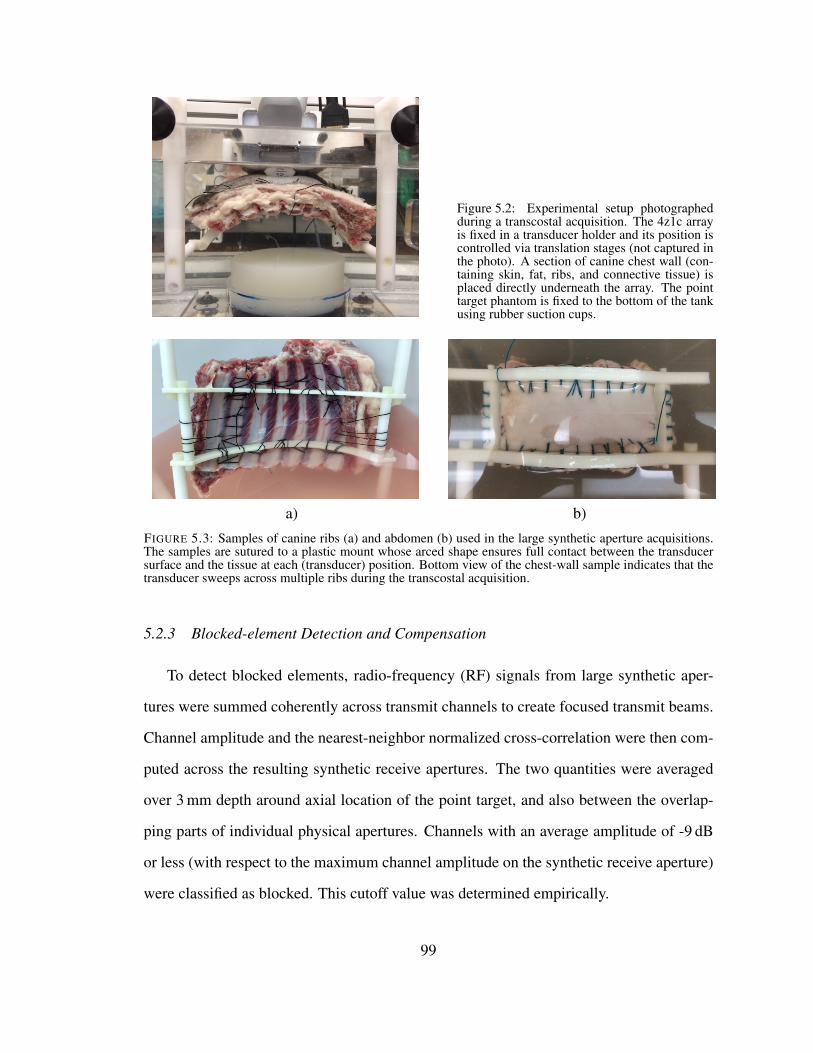
Figure 5.2: Experimental setup photographedduring a transcostal acquisition. The 4z1c arrayis fixed in a transducer holder and its position iscontrolled via translation stages (not captured inthe photo). A section of canine chest wall (con-taining skin, fat, ribs, and connective tissue) isplaced directly underneath the array. The pointtarget phantom is fixed to the bottom of the tankusing rubber suction cups.
a) b)
FIGURE 5.3: Samples of canine ribs (a) and abdomen (b) used in the large synthetic aperture acquisitions.The samples are sutured to a plastic mount whose arced shape ensures full contact between the transducersurface and the tissue at each (transducer) position. Bottom view of the chest-wall sample indicates that thetransducer sweeps across multiple ribs during the transcostal acquisition.
5.2.3 Blocked-element Detection and Compensation
To detect blocked elements, radio-frequency (RF) signals from large synthetic aper-
tures were summed coherently across transmit channels to create focused transmit beams.
Channel amplitude and the nearest-neighbor normalized cross-correlation were then com-
puted across the resulting synthetic receive apertures. The two quantities were averaged
over 3 mm depth around axial location of the point target, and also between the overlap-
ping parts of individual physical apertures. Channels with an average amplitude of -9 dB
or less (with respect to the maximum channel amplitude on the synthetic receive aperture)
were classified as blocked. This cutoff value was determined empirically.
99
To assess the impact of aperture size and (blocked-element) compensation methods on
image quality, B-mode images of point targets were beamformed using all, and subsets
of channels from the large synthetic aperture data sets. Specifically, for the transcostal
acquisitions, the images were beamformed:
1) by coherent summation of all channels,
2) by applying uniform weighting and coherent summation to the non-blocked chan-
nels only,
3) by applying adaptive weighting (and coherent summation) to the individual, non-
blocked Tx/Rx channel pairs,
4) and by compounding the intercostal sub-apertures.
In particular, for the adaptive blocked-element compensation, phase-aberration correction
was applied along with rescaling of the available Tx/Rx channel-pairs to recover the atten-
uated spatial frequencies. This method is presented in greater detail in section 5.2.4.
The PSFs created from the abdominal acquisition were used to indicate performance
of the beamforming methods under less severe imaging conditions. Due to the lack of
blocked elements, only full synthetic aperture and compounding were applied to the chan-
nel data. For each tissue image, a matching control image was created using the same
subsets of channels from the corresponding water-path acquisitions. Image quality was
characterized by full-width at half-maximum (FWHM) and side-lobe levels (SLL) of the
point spread functions, and by average clutter levels in the near-field.
5.2.4 Adaptive re-weighting of K-space
To adaptively compensate for the blocked channels, the remaining Tx/Rx channel pairs
were weighted to recover attenuated k-space frequencies and reduce associated side-lobes
in the PSF. The weights were determined following the convolution model of k-space
outlined by Walker and Trahey [118].
100
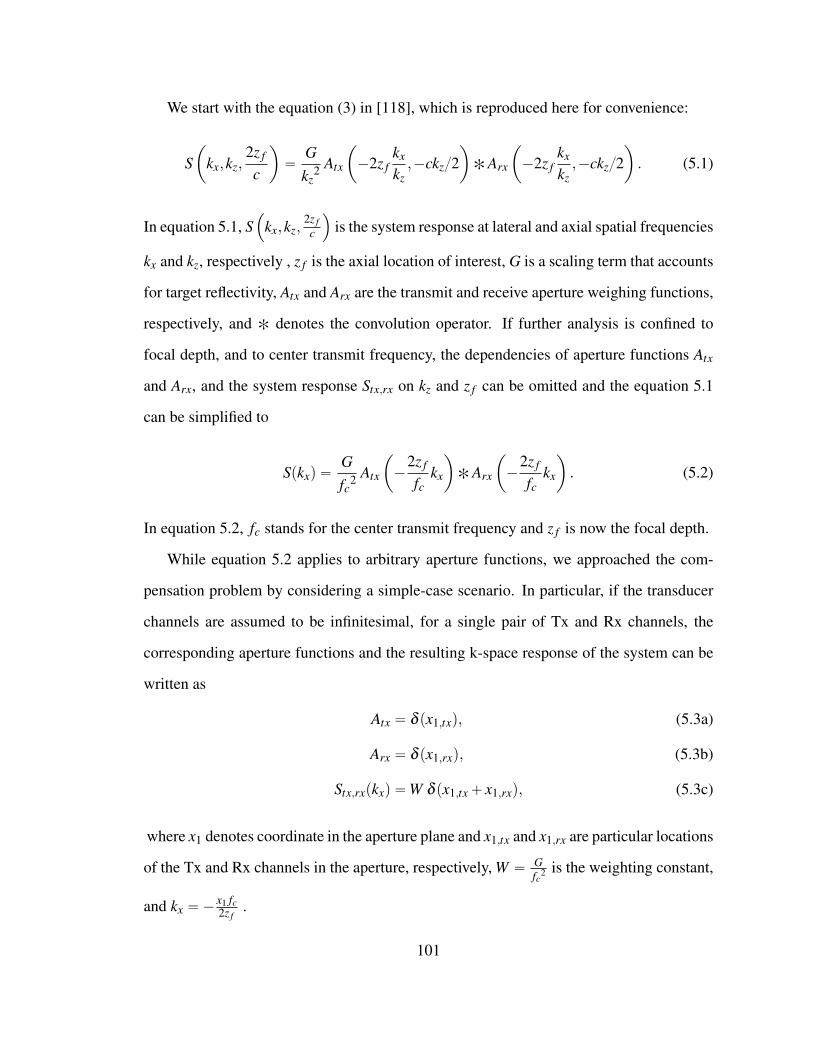
We start with the equation (3) in [118], which is reproduced here for convenience:
Sˆ
kx,kz,2z f
c
˙
“Gkz
2 Atx
ˆ
´2z fkx
kz,´ckz{2
˙
˚ Arx
ˆ
´2z fkx
kz,´ckz{2
˙
. (5.1)
In equation 5.1, S´
kx,kz,2z fc
¯
is the system response at lateral and axial spatial frequencies
kx and kz, respectively , z f is the axial location of interest, G is a scaling term that accounts
for target reflectivity, Atx and Arx are the transmit and receive aperture weighing functions,
respectively, and ˚ denotes the convolution operator. If further analysis is confined to
focal depth, and to center transmit frequency, the dependencies of aperture functions Atx
and Arx, and the system response Stx,rx on kz and z f can be omitted and the equation 5.1
can be simplified to
Spkxq “Gfc
2 Atx
ˆ
´2z f
fckx
˙
˚ Arx
ˆ
´2z f
fckx
˙
. (5.2)
In equation 5.2, fc stands for the center transmit frequency and z f is now the focal depth.
While equation 5.2 applies to arbitrary aperture functions, we approached the com-
pensation problem by considering a simple-case scenario. In particular, if the transducer
channels are assumed to be infinitesimal, for a single pair of Tx and Rx channels, the
corresponding aperture functions and the resulting k-space response of the system can be
written as
Atx “ δ px1,txq, (5.3a)
Arx “ δ px1,rxq, (5.3b)
Stx,rxpkxq “W δ px1,tx` x1,rxq, (5.3c)
where x1 denotes coordinate in the aperture plane and x1,tx and x1,rx are particular locations
of the Tx and Rx channels in the aperture, respectively, W “ Gfc2 is the weighting constant,
and kx “´x1 fc2z f
.
101

The k-space response of a multichannel system can be described as a sum of responses
from the individual Tx/Rx channel pairs:
Stotalpkxq “ÿ
tx,rxStx,rxplq | x1,tx` x1,rx “ l, (5.4)
where Stx,rx is rewritten as a function of sum of positions of Tx and Rx channels in the aper-
ture, l, and kx “ ´l fc{2z f . If the weighting constant W is assumed to be the same across
the aperture, then the total response Stotalpkxq is proportional to the number of available
Tx/Rx channel pairs at frequency kx. In a case of a missing (blocked) Tx/Rx channel pair,
the lack of its k-space response can be compensated by rescaling the remaining channel-
pair responses (at that frequency). In particular, the rescaling factor at spatial frequency kx
is computed as
RSpkxq “Stotalpkxq
Savailablepkxq, (5.5)
where Savailablepkxq and Stotalpkxq are the k-space responses of the apertures with and with-
out blocked channels, respectively.
To determine the individual channel-pair weights for the data acquisition setup de-
scribed in section 5.2.1, the k-space response for the large synthetic aperture was computed
from the individual physical apertures by utilizing the shifting property of convolution
[65]. First, blocked channels were detected following the procedure outlined in section
5.2.3. The blocked-channel maps for the individual apertures were then auto-convolved
and their respective k-space responses were shifted according to
Spkx`2∆x1fc
2z fq “ Atxpx1`∆x1q˚ Arxpx1`∆x1q. (5.6)
As stated in section 5.2.1, ∆x1 in equation 5.6 was incremented in half-of-the-transducer
length. The shifted k-space responses of the individual apertures were summed together to
synthesize a large-aperture k-space response. The rescaling factor was determined at each
102

spatial frequency of this response via equation 5.5. The weights for the channel-pairs in
the large synthetic aperture were re-mapped to the channel-pairs in individual apertures.
To ensure that the rescaled channel-pairs were adding in-phase and could recover atten-
uated frequencies, the arrival-time profiles estimated in section 5.2.5 for the transcostal
acquisition were applied to the non-blocked channels first.
5.2.5 Arrival-time Estimates
The large synthetic aperture data-sets collected on point targets through the ribs and
abdomen were also used to estimate the shape and magnitude of the respective tissue
induced aberrations. The arrival-time profiles were estimated from the channel data using
a least-squares method.
In the first step, focal delays were applied to the individual-channel signals to correct
for geometric path-length differences in the direction of the point target. Each signal
associated with a pair of transmit and receive channels could then be modeled as a delayed
version of the transmitted waveform ψ , corrupted with some additive noise
stx,rxptq “ ψpt`δtx,rxq` εchan. (5.7)
In equation 5.7, the signal stx,rx is in its time-continuous form, δtx,rx is a tissue-induced
delay associated with the pair of transmit and receive channels, and εchan accounts for
random-noise due to channel electronics. To find delays δtx,rx, the discrete signals were
cross-correlated with an estimate of the transmitted waveform
rtx,rxpmq “n2ÿ
n“n1
stx,rxpn`mqψpnq. (5.8)
In Equation 5.8, n and m are a sample number and lag value in time dimension, respec-
tively, and the difference n2´ n1 is on the order of wavelength. The reference waveform
ψ was obtained by averaging the focused point-target signals received across the aperture
103

in the control experiment. The channel signals stx,rx were temporally weighted by a de-
caying exponential centered around the estimated point-target depth. A 3-by-3-channel
moving-average window was also applied across the synthetic transmit aperture to reduce
the channel noise and improve cross-correlation estimates.
For each signal, the delay δtx,rx was estimated as the time-lag corresponding to the
maximum cross-correlation value
dtx,rx “ δtx,rx “ argmaxm
rtx,rxpmq ¨Ts (5.9)
where dtx,rx and Ts are used to denote the delay-estimate and sampling interval of the
signal, respectively. The measured signal delay can be expressed in terms of individual
delays on transmit and receive channels:
dtx,rx “ pttx` trxq´2tc` εd, (5.10)
dtx,rx “ pttx´ tcq`ptrx´ tcq` εd, (5.11)
dtx,rx “ ∆ttx`∆trx` εd, (5.12)
In equations 5.10 through 5.12, ttx and trx are times for a pulse to travel from the transmit
channel (to the point target), and (from the point target) to the receive channel, respectively,
2tc is the time of flight extracted from the reference waveform, and ∆ttx and ∆trx are the
tissue-induced delays on associated Tx and Rx channels that need to be estimated. εd is
a random delay-error caused by noise in the cross-correlation estimate. The equations for
all Tx/Rx channel-pairs can be written in the matrix form as
»
—
—
—
—
–
2 0 0 0 0 . . . 01 1 0 0 0 . . . 01 0 1 0 0 . . . 0. . . . . . . . . . . . . . . . . . .0 0 0 0 0 . . . 2
fi
ffi
ffi
ffi
ffi
fl
M
p180 ¨192qˆ192
»
—
—
—
—
—
–
∆t1∆t2∆t3
...∆t192
fi
ffi
ffi
ffi
ffi
ffi
fl
∆t
192ˆ1
`
»
—
—
—
—
—
–
ε1,1ε1,2ε1,3
...ε180,192
fi
ffi
ffi
ffi
ffi
ffi
fl
ε
p180 ¨192qˆ1
“
»
—
—
—
—
—
–
d1,1d1,2d1,3
...d180,192
fi
ffi
ffi
ffi
ffi
ffi
fl
d
p180 ¨192qˆ1
, (5.13)
104

where each row of model matrix M encodes a Tx/Rx channel pair, vectors d and ε con-
tain all measured signal delays and associated errors, respectively, and vector ∆t contains
tissue-induced delays for each channel. The dimensions of each vector and the matrix are
written underneath their respective symbols. The vector ∆t was estimated via the least-
squares solution
p∆t “ pMT Mq´1MT d. (5.14)
The Equations 5.8 through 5.14 were applied at each of the five physical-aperture
positions using the same reference waveform ψ . For the transcostal acquisition, blocked
channels were excluded from the arrival-time estimates. Arrival times estimates were also
obtained for wavefronts propagating through a water/alcohol-path only. These control
estimates were subtracted from the tissue estimates to obtain true aberrator profiles.
5.3 Results
5.3.1 Aperture-domain Signals
Signal information obtained from the individual channels of large synthetic apertures is
presented in Figures 5.4 through 5.6. Figure 5.4 shows channel amplitude and the nearest-
neighbor normalized cross-correlation for sample point-target acquisitions through excised
sections of canine ribs and abdomen, and for a control (point-target) acquisition through
the water path only. For all acquisitions, the two quantities are averaged over 3 mm depth
around axial location of the point target, and also between the overlapping parts of physical
(transducer) apertures. A moving-average window is applied to the resulting quantities
across the large synthetic apertures to further reduce the noise.3 Channel amplitude is
displayed on the decibel scale with the dynamic range adjusted to indicate the presence
of blocked elements. Cross-correlation is displayed using a linear color-map with the
3 Synthetic Tx and Rx aperture data was collected at five overlapping lateral transducer locations. Aperturesspanning the physical transducer surface at each of the five locations are referred to as physical apertures.An aperture spanning all five overlapping transducer positions is referred to as a large synthetic aperture.For more information on the SA data collection method, refer to section 5.2.1.
105

dynamic range from 0 to 1.
Two dark regions span along the elevation dimension in the amplitude and cross-
correlation images created from the transcostal acquisition; they are attributed to two ribs
blocking corresponding parts of the synthetic aperture. The shape of the blocked regions
is closely matched between the two images. Signal amplitude in the blocked regions is
on average 8 dB lower than the amplitude recorded on the remainder of the (virtual) array.
Overall, the amplitude and cross-correlation images created from the control and abdom-
inal acquisitions display a significantly higher degree of uniformity than their transcostal
counterparts. Lack of low values throughout the extent of the apertures implies that in both
cases, echoes have been received on all channels without significant obstruction. Only a
slight decrease in amplitude/cross-correlation, possibly due to a piece of connective tissue,
can be observed in the left side of synthetic aperture for the abdominal data set.
Binary aperture maps created by thresholding the channel amplitudes for the transcostal
acquisition in Figure 5.4 are shown in Figure 5.5. Channels with an average amplitude of
-9 dB or less (with respect to the maximum channel amplitude on the synthetic 2-D aper-
ture) are classified as blocked and are indicated in black color in the maps. The top map
shows positions of the blocked channels in the large synthetic aperture. The bottom five
maps are used to show positions of the blocked channels in the corresponding individual
physical apertures.
In the large synthetic aperture map, the chosen amplitude cutoff confines the blocked
channels to two regions that are observed in the corresponding amplitude and cross-
correlation images (Figure 5.4). The two regions combined occupy about a third of the
total synthetic-aperture size (x channels). In the physical aperture maps, shapes of the
blocked regions match between the overlapping parts of the apertures.4 The size of the
blocked regions varies between the individual apertures depending on their lateral location
4 The physical aperture maps are created from the positions of blocked channels in the large synthetic aper-ture. Overlapping parts of the individual apertures are therefore mapped using the same channel positionsfrom the large synthetic aperture.
106

on the chest-wall sample; the second, third, and fifth apertures are only partially blocked
on a single end, while the fourth physical aperture is centered on a rib and is almost com-
pletely blocked.
The k-space responses of large synthetic apertures with and without blocked channels
are shown in Figure 5.6. In all spectra, the spatial-frequency axes are expressed in terms
of shift indices assoicated with auto-convolution of the large 2-D aperture. All spectra
are normalized by the maximum of the desired response in b), and are displayed using
a linear color-map from 0 to 1. To create the k-space spectrum in Figure 5.6 a), the
individual aperture maps in Figure 5.5 were autoconvolved, so that each spatial frequency
is weighted by the number of available Tx/Rx channel pairs at the corresponding shift
value5. Due to presence of blocked channels, large regions of k-space in a) experience
significant attenuation. The k-space response of the equivalent synthetic aperture setup
in the absence of blocked channels is shown in Figure 5.6 b). The spectrum in b) has
the shape of a trapezoid in the lateral frequency dimension and the shape of a triangle
in the elevation frequency dimension. Figure 5.6 c) shows the k-space response obtained
after rescaling of the available Tx/Rx channel pairs in a), in order to compensate for the
blocked channels and approximate the desired response in b). Due to severe blockage,
at some spatial frequencies there are no available Tx/Rx channel pairs and the holes in
k-space remain.
5 For more information on how the large-aperture k-space spectra are created, the reader is referred tosection 5.2.4.
107

Amplitude Amplitude
lateral chan
ele
vation c
han
15 30 45
5
10
lateral chan
ele
vation c
han
15 30 45
5
10
ρ ρ
lateral chan
ele
vation c
han
15 30 45
5
10
lateral chan
ele
vation c
han
15 30 45
5
10
a) b)Amplitude
lateral chan
ele
vation c
han
15 30 45
5
10
ρ
lateral chan
ele
vation c
han
15 30 45
5
10
c)
FIGURE 5.4: The amplitude (top row) and nearest-neighbor normalized cross-correlation (bottom row) ofthe channel signals received across large synthetic 2-D apertures during an ex vivo transcostal acquisition(a), during its corresponding control acquisition (b), and during an abdominal acquisition (c). For all acqui-sitions, the synthetic aperture spans 5.76 cm (48 channels) in lateral and 1.44 cm (12 channels) in elevationdimension. Both amplitude and cross-correlation are averaged over 3 mm depth and a low-pass spatial filteris applied over the extent of the aperture to further reduce the noise. Channel amplitude is displayed on thedecibel scale from -11 to 0, while cross-correlation is displayed using a linear color-map with the dynamicrange from 0 to 1. For the transcostal acquisition, regions of low values are attributed to ribs blocking thoseparts of the aperture. Shape of the blocked regions matches between the amplitude and cross-correlationimages. For the control acquisition, amplitude and cross-correlation display high values throughout the ex-tent of the aperture indicating echoes have been received on all channels without significant obstruction. Forthe abdominal acquisition, there is a slight loss of channel amplitude/cross-correlation on the left side of thesynthetic aperture, potentially caused by a piece of connective tissue.
108

ele
vation c
han
Blocked channels
lateral chan
5 10 15 20 25 30 35 40 45
5
10
ele
vation c
han
Blocked Tx channels
5
10
ele
vation c
han
5
10
ele
vation c
han
5
10
ele
vation c
han
5
10
ele
vation c
han
lateral chan
5 10 15
5
10
109

FIGURE 5.5 (preceding page): Binary aperture maps obtained by thresholding channel amplitudes for thetranscostal acquisition displayed in Figure 5.4 (the upper left image). Black color is used to indicate posi-tions of blocked channels in the full synthetic aperture (top map) and in the individual physical-transducerapertures that are used to create the synthetic aperture (bottom five maps).
Blocked Control
xtx
+ xrx
ytx
+ y
rx
30 60 90
10
20
xtx
+ xrx
ytx
+ y
rx
30 60 90
10
20
a) b)Re-scaled
xtx
+ xrx
ytx
+ y
rx
30 60 90
10
20
c)
FIGURE 5.6: The system response in k-space derived from the binary aperture maps in Figure 5.5 (a), thematching k-space response in the absence of blocked elements (b), and the k-space response obtained afterrescaling of the non-blocked Tx/Rx channel-pairs in a) to approximate the desired response in b) (c). Allimages are normalized by the maximum of the desired k-space response in b), and are displayed on a linearscale from 0 to 1. Spatial frequencies in x and y axes are expressed as shift-indices associated with theauto-convolution of the large 2-D aperture. Blocked channels cause a loss of spatial-frequency amplitudes.At spatial frequencies for which all the corresponding Tx/Rx channel-pairs are blocked, holes in k-spaceremain after rescaling.
110

5.3.2 Compensated B-mode images
Examples of B-mode images of point targets and reverberation clutter reconstructed
from the large synthetic aperture data are shown together with the supporting plots in
Figures 5.7 through 5.16. The images are created from the same transcostal and abdom-
inal acquisitions as the images of channel amplitude and cross-correlation in Figure 5.4.
All B-mode images are reconstructed in the plane of transducer motion, along the lateral
dimension at zero elevation coordinate (i.e. middle lateral slices). Since the elevation di-
mension of the synthetic aperture is four times smaller (than its lateral dimension), and is
parallel to the ribs for the transcostal acquisition, the analysis of the point-spread functions
in this dimension does not offer any new insights and is omitted. The B-mode images are
displayed on the decibel scale with the dynamic range from -50 to 0.
Point target images created from the transcostal acquisition and its corresponding con-
trol are presented in Figures 5.7 and 5.8. The images from the transcostal acquisition in
Figure 5.7 are created, from left to right:
1) by coherently summing signals from all the channels (full synthetic aperture method),
2) by applying uniform weighting and coherent summation to the non-blocked chan-
nels only (synthetic aperture with basic compensation),
3) by turning off the blocked channels, and applying phase-aberration correction and
rescaling to the non-blocked Tx/Rx channel-pairs to approximate a desired response
in k-space (synthetic aperture with adaptive compensation), and
4) by compounding the apertures that span the intercostal spaces.
For all compensation methods, the blocked channels are identified and turned off following
the maps in Figure 5.5. For the adaptive compensation method, phase-aberration correc-
tion is implemented using the arrival-time profile in Figure 5.17, top. The control images
in Figure 5.7 are beamformed using the same methods and subsets of channels as their
corresponding transcostal images, but from the synthetic aperture data acquired through
111

SA
lateral (mm)
axia
l (m
m)
−8 −4 0 4 8
83
85
87
SA w/ basic compensation
lateral (mm)
−8 −4 0 4 8
SA w/ adaptive compensation
lateral (mm)
−8 −4 0 4 8
Compounded Aperture
lateral (mm)
−8 −4 0 4 8
SA
lateral (mm)
axia
l (m
m)
−8 −4 0 4 8
83
85
87
SA w/ elements off
lateral (mm)
−8 −4 0 4 8
SA w/ adaptive compensation
lateral (mm)
−8 −4 0 4 8
Compounded Aperture
lateral (mm)
−8 −4 0 4 8
FIGURE 5.7: B-mode images of point targets created with and without different blocked-element com-pensation schemes applied to the channel data from the transcostal acquisition (top) and from the controlacquisition (bottom). For the transcostal acquisition, images are reconstructed, from left to right: by coher-ently summing signals from all the channels (synthetic aperture method), by applying uniform weightingand coherent summation to non-blocked channels only (synthetic aperture with basic compensation), byphase-correcting and adaptively weighting non-blocked channel signals to approximate a desired responsein k-space (synthetic aperture with adaptive compensation), and by compounding the apertures that spanintercostal spaces. For the latter three beamforming methods, the blocked channels are selectively turnedoff on both Tx and Rx following the maps in Figure 5.5. For the control acquisition, point target images arebeamformed using the same methods and subsets of channels as for the transcostal acquisition. The PSFscreated from the transcostal acquisition show higher sidelobes and are wider than their control counterparts.For the transcostal acquisition, just turning off the blocked channels does not significantly alter the shape ofthe synthetic aperture PSF. For both data sets, adaptive blocked-element compensation significantly reducessidelobes induced by aperture sparsity. Compounding also reduces sidelobes but at the expense of increasedmainlobe width for both acquisitions. All images are displayed on the decibel scale with the dynamic rangefrom -50 to 0.
a water-path only. The individual images used for compounding for both acquisitions
are shown in Figure 5.8; the resulting compounded images are displayed again to allow
side-by-side comparison. To further facilitate comparison of the point-spread-functions
(PSF) across beamforming methods and aperture sizes, the corresponding beamplots are
presented in Figure 5.9.6
The PSFs created from the transcostal acquisition show significantly higher sidelobe
levels (SLL) and larger effective full-width at half maximum (FWHM) than their control
counterparts. In particular, for the full synthetic aperture PSFs, going from the control to
the transcostal acquisition, SLL increases by 15.1 dB and FWHM increases by a factor
of 6.2 7. Further, when the uniform channel-weighting is applied to transcostal data, the
6 Beamplots refer to lateral amplitude profiles taken at the point target depth.7 Such a large increase in the effective width of the full-synthetic-aperture PSF is due to high sidelobes in
112
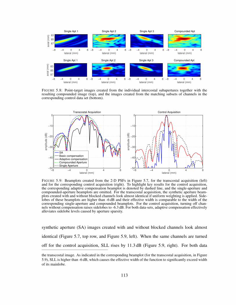
Single Apt 1
lateral (mm)
axia
l (m
m)
−8 −4 0 4 8
83
85
87
Single Apt 2
lateral (mm)
−8 −4 0 4 8
Single Apt 3
lateral (mm)
−8 −4 0 4 8
Compounded Apt
lateral (mm)
−8 −4 0 4 8
Single Apt 1
lateral (mm)
axia
l (m
m)
−8 −4 0 4 8
83
85
87
Single Apt 2
lateral (mm)
−8 −4 0 4 8
Single Apt 3
lateral (mm)
−8 −4 0 4 8
Compounded Apt
lateral (mm)
−8 −4 0 4 8
FIGURE 5.8: Point-target images created from the individual intercostal subapertures together with theresulting compounded image (top), and the images created from the matching subsets of channels in thecorresponding control data set (bottom).
−8 −4 0 4 8−50
−40
−30
−20
−10
0Transcostal Acquisition
lateral (mm)
am
plit
ud
e (
dB
)
SA
Basic compensation
Adaptive compensation
Compounded Aperture
Single Aperture
−8 −4 0 4 8−50
−40
−30
−20
−10
0Control Acquisition
lateral (mm)
am
plit
ud
e (
dB
)
FIGURE 5.9: Beamplots created from the 2-D PSFs in Figure 5.7, for the transcostal acquisition (left)and for the corresponding control acquisition (right). To highlight key results for the control acquisition,the corresponding adaptive compensation beamplot is denoted by dashed line, and the single-aperture andcompounded-aperture beamplots are omitted. For the transcostal acquisition, the synthetic aperture beam-plots created with and without blocked channels look almost identical if uniform weighting is applied. Side-lobes of these beamplots are higher than -6 dB and their effective width is comparable to the width of thecorresponding single-aperture and compounded beamplots. For the control acquisition, turning off chan-nels without compensation raises sidelobes to -6.3 dB. For both data-sets, adaptive compensation effectivelyalleviates sidelobe levels caused by aperture sparsity.
synthetic aperture (SA) images created with and without blocked channels look almost
identical (Figure 5.7, top row, and Figure 5.9, left). When the same channels are turned
off for the control acquisition, SLL rises by 11.3 dB (Figure 5.9, right). For both data
the transcostal image. As indicated in the corresponding beamplot (for the transcostal acquisition, in Figure5.9), SLL is higher than -6 dB, which causes the effective width of the function to significantly exceed widthof its mainlobe.
113
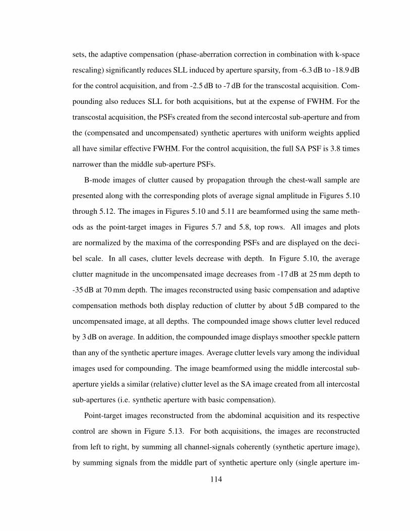
sets, the adaptive compensation (phase-aberration correction in combination with k-space
rescaling) significantly reduces SLL induced by aperture sparsity, from -6.3 dB to -18.9 dB
for the control acquisition, and from -2.5 dB to -7 dB for the transcostal acquisition. Com-
pounding also reduces SLL for both acquisitions, but at the expense of FWHM. For the
transcostal acquisition, the PSFs created from the second intercostal sub-aperture and from
the (compensated and uncompensated) synthetic apertures with uniform weights applied
all have similar effective FWHM. For the control acquisition, the full SA PSF is 3.8 times
narrower than the middle sub-aperture PSFs.
B-mode images of clutter caused by propagation through the chest-wall sample are
presented along with the corresponding plots of average signal amplitude in Figures 5.10
through 5.12. The images in Figures 5.10 and 5.11 are beamformed using the same meth-
ods as the point-target images in Figures 5.7 and 5.8, top rows. All images and plots
are normalized by the maxima of the corresponding PSFs and are displayed on the deci-
bel scale. In all cases, clutter levels decrease with depth. In Figure 5.10, the average
clutter magnitude in the uncompensated image decreases from -17 dB at 25 mm depth to
-35 dB at 70 mm depth. The images reconstructed using basic compensation and adaptive
compensation methods both display reduction of clutter by about 5 dB compared to the
uncompensated image, at all depths. The compounded image shows clutter level reduced
by 3 dB on average. In addition, the compounded image displays smoother speckle pattern
than any of the synthetic aperture images. Average clutter levels vary among the individual
images used for compounding. The image beamformed using the middle intercostal sub-
aperture yields a similar (relative) clutter level as the SA image created from all intercostal
sub-apertures (i.e. synthetic aperture with basic compensation).
Point-target images reconstructed from the abdominal acquisition and its respective
control are shown in Figure 5.13. For both acquisitions, the images are reconstructed
from left to right, by summing all channel-signals coherently (synthetic aperture image),
by summing signals from the middle part of synthetic aperture only (single aperture im-
114

SA
lateral (mm)
axia
l (m
m)
−8 −4 0 4 8
20
40
60
SA w/ basic compensation
lateral (mm)
−8 −4 0 4 8
SA w/ adaptive compensation
lateral (mm)
−8 −4 0 4 8
Compounded Aperture
lateral (mm)
−8 −4 0 4 8
FIGURE 5.10: B-mode images displaying clutter levels before and after blocked-element compensationis applied to the synthetic aperture data acquired through a ribs sample. The transcostal acquisition andbeamforming schemes used to create images match those of Figure 5.7. In all cases, clutter magnitudedecreases moving away from the ribs. Compounded and sythetic aperture images beamformed without theblocked channels show reduced clutter compared to the (sythetic aperture) image beamformed using all thechannels. All images are displayed on the decibel scale with the dynamic range from -50 to 0.
age), and by compounding.8 The corresponding beamplots are presented in Figure 5.14.
The PSFs created from the abdominal acquisition show small changes compared to their
matching control images; SLL changes are within 5 dB while the mainlobe width increases
at most by a factor of 1.2. For both acquisitions, the mainlobe is the narrowest in the syn-
thetic aperture image while the single-aperture and compounded images display similar
mainlobe width. Going from the single aperture to synthetic aperture images mainlobe
width decreases by a factor of 3.4 for the control acquisition and by a factor of 2.7 for the
8 The shape of subapertures used to create the single-aperture and compounded images matches the inter-costal spaces, plus the adjacent blocked channels, from a transcostal acquisition. This allows for a directcomparison between the point target images generated from the abdominal and transcostal acquisitions.
115

Single Apt 1
lateral (mm)
axia
l (m
m)
−8 −4 0 4 8
20
40
60
Single Apt 2
lateral (mm)
−8 −4 0 4 8
Single Apt 3
lateral (mm)
−8 −4 0 4 8
Compounded Apt
lateral (mm)
−8 −4 0 4 8
FIGURE 5.11: Individual B-mode images of clutter used to create the compounded image in Figure 5.10,which is displayed again for clarity. Each image is normalized with respect to the maximum brightness valueof the compounded point target image (the top leftmost image in Figure 5.8). In all cases, clutter magnitudedecreases moving away from the ribs. The image generated from the second intercostal aperture contributesthe highest amount of clutter to the compounded image.
abdominal acquisition.
Figures 5.15 and 5.16 show B-mode images of clutter due to propagation through the
section of abdominal wall, and supporting plots of average clutter magnitude as a function
of depth, respectively. The B-mode images (and their respective plots) are reconstructed
using the same subsets of channels as the point target images in Figure 5.13. Overall, the
clutter levels are relatively low, not exceeding -40 dB at 20 mm depth and monotonically
decreasing. The compounded image displays the highest level of clutter; its average clutter
magnitude is about 5 dB higher than that of the synthetic aperture and single aperture
images.
116
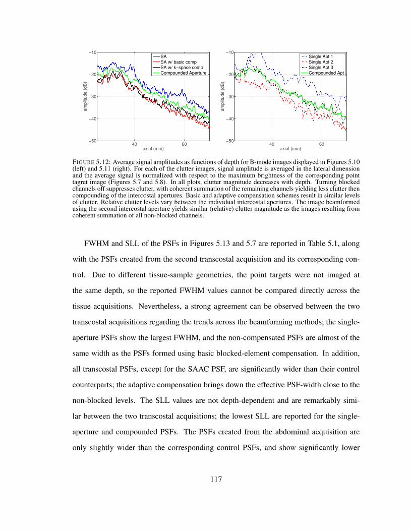
40 60−50
−40
−30
−20
−10
am
plit
ude (
dB
)
axial (mm)
SA
SA w/ basic comp
SA w/ k−space comp
Compounded Aperture
40 60−50
−40
−30
−20
−10
am
plit
ude (
dB
)
axial (mm)
Single Apt 1
Single Apt 2
Single Apt 3
Compounded Apt
FIGURE 5.12: Average signal amplitudes as functions of depth for B-mode images displayed in Figures 5.10(left) and 5.11 (right). For each of the clutter images, signal amplitude is averaged in the lateral dimensionand the average signal is normalized with respect to the maximum brightness of the corresponding pointtagret image (Figures 5.7 and 5.8). In all plots, clutter magnitude decreases with depth. Turning blockedchannels off suppresses clutter, with coherent summation of the remaining channels yielding less clutter thencompounding of the intercostal apertures. Basic and adaptive compensation schemes result in similar levelsof clutter. Relative clutter levels vary between the individual intercostal apertures. The image beamformedusing the second intercostal aperture yields similar (relative) clutter magnitude as the images resulting fromcoherent summation of all non-blocked channels.
FWHM and SLL of the PSFs in Figures 5.13 and 5.7 are reported in Table 5.1, along
with the PSFs created from the second transcostal acquisition and its corresponding con-
trol. Due to different tissue-sample geometries, the point targets were not imaged at
the same depth, so the reported FWHM values cannot be compared directly across the
tissue acquisitions. Nevertheless, a strong agreement can be observed between the two
transcostal acquisitions regarding the trends across the beamforming methods; the single-
aperture PSFs show the largest FWHM, and the non-compensated PSFs are almost of the
same width as the PSFs formed using basic blocked-element compensation. In addition,
all transcostal PSFs, except for the SAAC PSF, are significantly wider than their control
counterparts; the adaptive compensation brings down the effective PSF-width close to the
non-blocked levels. The SLL values are not depth-dependent and are remarkably simi-
lar between the two transcostal acquisitions; the lowest SLL are reported for the single-
aperture and compounded PSFs. The PSFs created from the abdominal acquisition are
only slightly wider than the corresponding control PSFs, and show significantly lower
117

SA
lateral (mm)
axia
l (m
m)
−8 −4 0 4 8
67
69
71
Single Apt 2
lateral (mm)
−8 −4 0 4 8
Compounded Aperture
lateral (mm)
−8 −4 0 4 8
SA
lateral (mm)
axia
l (m
m)
−8 −4 0 4 8
67
69
71
Single Apt 2
lateral (mm)
−8 −4 0 4 8
Compounded Aperture
lateral (mm)
−8 −4 0 4 8
FIGURE 5.13: Point-target images created using different subsets of channels from a large synthetic aper-ture data set collected through the abdomen (top) and from the data collected in the corresponding controlacquisition (bottom). For both acquisitions, images are reconstucted, from left to right: by coherently sum-ming signals from all the channels (synthetic aperture method), by coherently summing signals from themiddle part of the synthetic aperture only, and by compounding the apertures that match intercostal spacesin the corresponding transcostal acquisition. The images reconstructed from the abdominal acquisition dis-play slightly higher sidelobe levels than the corresponding control images. For both acquisitions, the middle(sub)aperture and compounded images show increased mainlobe width compared to the full synthetic aper-ture images. All images are displayed on the decibel scale with the dynamic range from -50 to 0.
−8 −4 0 4 8−50
−40
−30
−20
−10
0Abdominal Acquisition
lateral (mm)
am
plit
ud
e (
dB
)
SA
Compounded
Single Aperture
−8 −4 0 4 8−50
−40
−30
−20
−10
0Control Acquisition
lateral (mm)
am
plit
ud
e (
dB
)
FIGURE 5.14: Beamplots created from the 2-D PSFs in Figure 5.13, for the abdominal acquisition (left) andfor its corresponding control acquisition (right). While beamplots created from the abdominal acquisitionappear asymmetric and distorted compared to their control counterparts, the mainlobe width and the sidelobelevels do not change significantly between the two acquisitions. For both acquisitions, the compounded andsingle-aperture beamplots have similar mainlobe width; the beamwidth is the smallest for the syntheticaperture plots.
SLL compared to their transcostal counterparts.
118
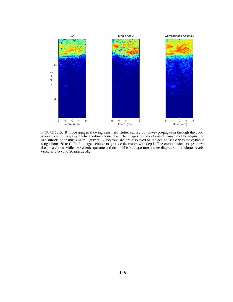
SA
lateral (mm)
axia
l (m
m)
−8 −4 0 4 8
20
40
Single Apt 2
lateral (mm)
−8 −4 0 4 8
Compounded Aperture
lateral (mm)
−8 −4 0 4 8
FIGURE 5.15: B-mode images showing near-field clutter caused by (wave) propagation through the abdo-mainal layer during a synthetic aperture acquisition. The images are beamformed using the same acquisitionand subsets of channels as in Figure 5.13, top row, and are displayed on the decibel scale with the dynamicrange from -50 to 0. In all images, clutter magnitude decreases with depth. The compounded image showsthe most clutter while the sythetic aperture and the middle (sub)aperture images display similar clutter levels,especially beyond 20 mm depth.
119

20 40−70
−60
−50
−40
−30
am
plit
ude (
dB
)
axial (mm)
SA
Single Apt 2
Compounded Aperture
FIGURE 5.16: Average clutter magnitude as a function of depth for B-mode images in Figure 5.15. Foreach image of clutter, the magnitude is integrated along the lateral dimension and is normalized with respectto the maximum brightness of the corresponding point tagret image (Figure 5.13). The compounded imageyields the highest level of clutter. Relative clutter levels measured in the full syntethic aperture image arealmost the same as those in the middle-aperture image. For all beamforming methods, the clutter magnitudeis monotonically decreasing and does not exceed -30 dB.
120
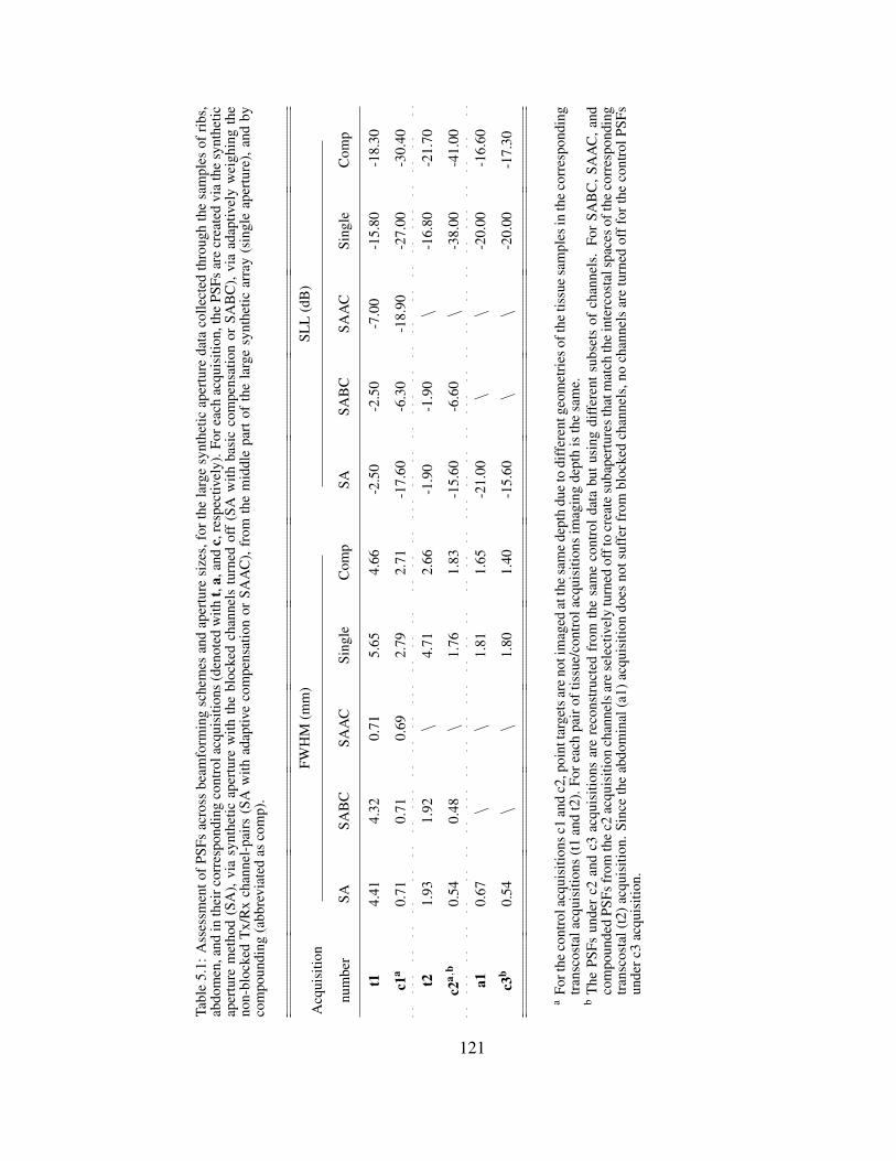
Tabl
e5.
1:A
sses
smen
tof
PSFs
acro
ssbe
amfo
rmin
gsc
hem
esan
dap
ertu
resi
zes,
for
the
larg
esy
nthe
ticap
ertu
reda
taco
llect
edth
roug
hth
esa
mpl
esof
ribs
,ab
dom
en,a
ndin
thei
rcor
resp
ondi
ngco
ntro
lacq
uisi
tions
(den
oted
with
t,a,
and
c,re
spec
tivel
y).F
orea
chac
quis
ition
,the
PSFs
are
crea
ted
via
the
synt
hetic
aper
ture
met
hod
(SA
),vi
asy
nthe
ticap
ertu
rew
ithth
ebl
ocke
dch
anne
lstu
rned
off
(SA
with
basi
cco
mpe
nsat
ion
orSA
BC
),vi
aad
aptiv
ely
wei
ghin
gth
eno
n-bl
ocke
dT
x/R
xch
anne
l-pa
irs
(SA
with
adap
tive
com
pens
atio
nor
SAA
C),
from
the
mid
dle
part
ofth
ela
rge
synt
hetic
arra
y(s
ingl
eap
ertu
re),
and
byco
mpo
undi
ng(a
bbre
viat
edas
com
p).
Acq
uisi
tion
num
ber
FWH
M(m
m)
SLL
(dB
)
SASA
BC
SAA
CSi
ngle
Com
pSA
SAB
CSA
AC
Sing
leC
omp
t14.
414.
320.
715.
654.
66-2
.50
-2.5
0-7
.00
-15.
80-1
8.30
c1a
0.71
0.71
0.69
2.79
2.71
-17.
60-6
.30
-18.
90-2
7.00
-30.
40
t21.
931.
92\
4.71
2.66
-1.9
0-1
.90
\-1
6.80
-21.
70
c2a,
b0.
540.
48\
1.76
1.83
-15.
60-6
.60
\-3
8.00
-41.
00
a10.
67\
\1.
811.
65-2
1.00
\\
-20.
00-1
6.60
c3b
0.54
\\
1.80
1.40
-15.
60\
\-2
0.00
-17.
30
aFo
rthe
cont
rola
cqui
sitio
nsc1
and
c2,p
oint
targ
etsa
reno
tim
aged
atth
esa
me
dept
hdu
eto
diff
eren
tgeo
met
ries
ofth
etis
sue
sam
ples
inth
eco
rres
pond
ing
tran
scos
tala
cqui
sitio
ns(t
1an
dt2
).Fo
reac
hpa
irof
tissu
e/co
ntro
lacq
uisi
tions
imag
ing
dept
his
the
sam
e.b
The
PSFs
unde
rc2
and
c3ac
quis
ition
sar
ere
cons
truc
ted
from
the
sam
eco
ntro
ldat
abu
tusi
ngdi
ffer
ents
ubse
tsof
chan
nels
.Fo
rSA
BC
,SA
AC
,and
com
poun
ded
PSFs
from
the
c2ac
quis
ition
chan
nels
are
sele
ctiv
ely
turn
edof
fto
crea
tesu
bape
rtur
esth
atm
atch
the
inte
rcos
tals
pace
sof
the
corr
espo
ndin
gtr
ansc
osta
l(t2
)acq
uisi
tion.
Sinc
eth
eab
dom
inal
(a1)
acqu
isiti
ondo
esno
tsuf
ferf
rom
bloc
ked
chan
nels
,no
chan
nels
are
turn
edof
ffor
the
cont
rolP
SFs
unde
rc3
acqu
isiti
on.
121

5.3.3 Arrival-time Profiles
Time-of-arrival estimates for the wavefronts originating from a point target and prop-
agating through samples of ribs, abdomen, and water-path only are shown in Figure 5.17.
The estimates are obtained across large synthetic apertures and from the same acquisitions
used to create images of channel data and B-mode images in Sections 5.3.1 and 5.3.2,
respectively. For all acquisitions, the synthetic receive aperture is composed of five over-
lapping physical aperture positions and it spans 48 channels in the lateral and 12 channels
in the elevation dimension. The color of arrival-time surface is mapped to the surface
height with low negative values colored in dark blue and high positive values colored in
bright red.
For the transcostal acquisition, the blocked channels are omitted from the arrival-time
profile following the binary maps in Figure 5.5. The arrival-time surface over the inter-
costal spaces indicates a high magnitude, low frequency aberrator. The estimated aberrator
for the abdominal wall is of lower magnitude than its intercostal counterpart, except for
the peak-estimate on the left side of synthetic array. Wavefront distortions due to propaga-
tion through water only are minimal as seen in the control profile. The root-mean-square
(rms) values of arrival-time profiles are computed to be 58 ns for the transcostal acquisi-
tion, 24.8 ns for the abdominal acquisition, and 10.8 ns for the control acquisition at the
transmit frequency of 2.5 MHz. For all acquisitions, there is a strong agreement between
the arrival-time estimates from the overlapping aperture positions.
122
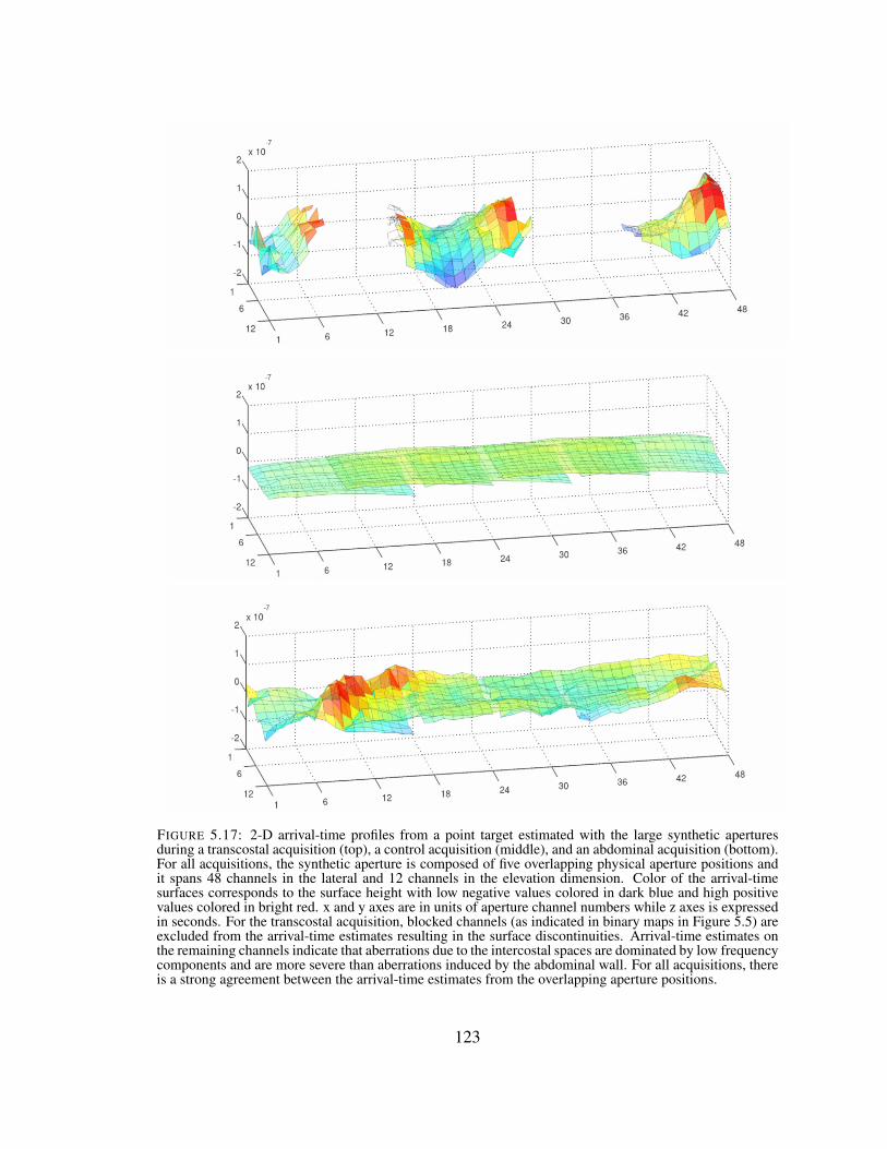
FIGURE 5.17: 2-D arrival-time profiles from a point target estimated with the large synthetic aperturesduring a transcostal acquisition (top), a control acquisition (middle), and an abdominal acquisition (bottom).For all acquisitions, the synthetic aperture is composed of five overlapping physical aperture positions andit spans 48 channels in the lateral and 12 channels in the elevation dimension. Color of the arrival-timesurfaces corresponds to the surface height with low negative values colored in dark blue and high positivevalues colored in bright red. x and y axes are in units of aperture channel numbers while z axes is expressedin seconds. For the transcostal acquisition, blocked channels (as indicated in binary maps in Figure 5.5) areexcluded from the arrival-time estimates resulting in the surface discontinuities. Arrival-time estimates onthe remaining channels indicate that aberrations due to the intercostal spaces are dominated by low frequencycomponents and are more severe than aberrations induced by the abdominal wall. For all acquisitions, thereis a strong agreement between the arrival-time estimates from the overlapping aperture positions.
123

5.4 Discussion
5.4.1 Blocked-element Detection in Large Coherent Apertures
The point-spread functions and arrival-time profiles demonstrate that large transmit
and receive apertures have been successfully synthesized from the individual transducer
apertures at different lateral positions. The full-synthetic-aperture PSFs created from the
control acquisitions are symmetric and display reduced mainlobe width when compared
to their individual-aperture counterparts (Figures 5.9 and 5.14). In addition, for all acqui-
sitions, there is a strong agreement between the arrival-time estimates obtained from the
overlapping parts of individual apertures (Figure 5.17). Both observations confirm cor-
rect spatial registration of individual transducer apertures and adequate geometric delays
applied to all channel signals.
Blocked-element detection algorithm introduced in Chapter 4 has been successfully
applied to large synthetic apertures used to image through rib samples ex vivo. The
large-aperture binary map in Figure 5.5, which was created by thresholding the channel-
amplitude image for the transcostal acquisition in Figure 5.4 clearly conveys the extent
of the regions blocked by bone. On the other hand, the channel-amplitude and cross-
correlation images created from the abdominal and control acquisitions display relative
uniformity in the absence of acoustic obstacles (Figure 5.4); thresholding them is not ex-
pected to discriminate any signal features on the 2-D aperture.
5.4.2 Image Degradation due to Blocked Elements
Comparing clutter levels and PSFs across the tissue acquisitions and their respective
controls, ultrasound propagation through the chest wall causes significantly more image
degradation than propagation through the abdomen. Reverberation clutter due to chest
wall is measured to be approximately -20 dB at 2 cm away from the tissue, and is 20 -
25 dB higher (depending on the depth) than its abdominal counterpart (Figures 5.12 and
124

5.16). Further, comparing the uncompensated transcostal PSFs to the full SA PSFs from
the matching control acquisitions, SLL increases by as much as 15.1 dB, putting it above
-6 dB for both transcostal acquisitions (Figure 5.9 and Table 5.1). As a result, the effec-
tive FWHM of the uncompensated transcostal PSFs is four to six times larger than their
mainlobe width, and than the FWHM of the above-mentioned control PSFs. In contrast,
wave propagation through the abdomen causes sidelobes (of the full SA PSF) to increase
by 5.4 dB and the FWHM to increase by a factor of 1.2 (Figure 5.14 and Table 5.1).
Sparsity of the aperture due to blocked elements is estimated as a dominant source
of high SLL for the transcostal acquisitions. To isolate the degradation of focus due to
blocked elements from the effects of phase aberration, reverberation, and other sources of
acoustic noise, the blocked-channel map in Figure 5.5 was used to turn off channels in the
corresponding control acquisition. The resulting increase in SLL is 11.3 dB, which makes
up majority of the total increase in SLL measured for the transcostal acquisition (15.1 dB)
(Figures 5.7 and 5.9 and Table 5.1). For the imaged rib configuration (and the resulting
distribution of blocked channels), appearance of two sidelobes of such high magnitude is
consistent with the simulation and ex vivo results presented in [62] and [7]9.
For large arrays that employ conventional beamforming, aperture sparsity due to peri-
odic rib structure can forfeit expected improvements in resolution. Going from a single-
intercostal-subaperture PSF to the full SA PSF, SLL increases by at least 13 dB and the
effective FWHM decreases by a factor of 1.3 and 2.4 for the first and second transcostal
acquisitions, respectively (Figure 5.9 and Table 5.1). In contrast, for the abdominal acqui-
sition, in the absence of acoustic obstacles, the decrease in FWHM is comparable to the
increase in overall aperture size while SLL does not change significantly in the process.
Comparing the PSF reconstructed using the middle third of the aperture to the full SA
PSF, FWHM decreases by a factor of 2.7 while SLL stays close to -20 dB (Figure 5.14 and
9 In particular, according to simulations results in [62], when the aperture captures multiple ribs, and widthof a rib and the intercostal space are almost identical, the number of maxima observed in the beampatternwill be three, one at the focus and one at each side. Furthermore, side peaks are estimated at -4 dB.
125

Table 5.1).
5.4.3 Impact of Phase Aberration
While phase aberration due to chest wall is not the main contributor to the loss of focus
quality in transcostal ultrasound, it is significantly stronger than its abdominal counterpart.
The rms values of arrival-time profiles are 58 ns for the transcostal acquisition and 24.8 ns
for the abdominal acquisition (Figure 5.17). The rms arrival-time value obtained for the
transcostal acquisition is much larger than the average rms value reported by Hinkelman
et al.10 [51]. In addition to using different types of tissue for the ex vivo measurements
(canine v.s. human chest-wall samples), discrepancy in results can be explained by the
choice of tissue-regions over which the arrival-time profiles are reconstructed in each
study. The arrival-time estimates in Figure 5.17 are particularly large near the blocked
channels reaching extrema of ˘100 ns, which can be attributed to cartilage and connec-
tive tissue surrounding the bone. In [51], the receive apertures are windowed specifically
to omit areas over bone and costal cartilage, and to isolate distortions introduced by soft-
tissue inhomogeneities. As most of the arrival-time measurements are made near the center
of intercostal spaces the average rms value is lower.
5.4.4 Efficacy of Compensation Methods
We have demonstrated that adaptive blocked-element compensation (i.e. phase aberra-
tion correction in combination with k-space rescaling) has a potential to reduce near-field
clutter and restore point-resolution of large apertures in the presence of blocked elements.
Turning off blocked channels in transmit and receive apertures reduces clutter noise in
transthoracic images by as much as 5 dB, when the (remaining) intercostal sub-apertures
are coherently summed (Figures 5.10 and 5.12). Further, in the presence of aperture spar-
sity, adaptive weighing of the non-blocked channels rescales attenuated k-space frequen-
10 Hinkelman et al. measured the arrival-time fluctuations in 16 intercostal spaces to obtain the average rmsvalue of 21.3 ns [51].
126

cies and reduces SLL by 5 dB for the transcostal acquisition, and by 12.6 dB for its match-
ing control acquisition (Figure 5.7 and Table 5.1). For the transcostal acquisition, bringing
the SLL bellow -6 dB (to -7 dB in this case) restores the effective width of the PSF to the
FWHM of its mainlobe, which implies a 6-fold improvement in lateral resolution (Table
5.1). Side-lobe reduction via k-space rescaling is not as effective for the transcostal acqui-
sition as it is for the control, since acoustic noise on the non-blocked channels introduces
random variations in the k-space spectrum (of the sparse aperture) [118], making it more
difficult to approximate the desired response. Phase-aberration correction only partially
addresses this problem.
Other compensation methods yield partial improvements of image quality. When the
blocked channels are turned off and the non-blocked channels are uniformly weighted (i.e.
basic compensation), the PSFs remain virtually unchanged. This can be attributed to lower
signal-amplitude on the blocked channels; while turning off those channels will reduce the
noise level, it will not significantly impact the shape of higher amplitude mainlobe and
sidelobes. Compounding the intercostal sub-apertures results in partial reduction of clut-
ter; measured decrease in average clutter level for the transcostal acquisition in Figure
5.10 is about 3 dB. However, speckle/noise texture in the compounded images appears
smoother than in the matching synthetic aperture images. In addition, compounding the
associated PSFs reduces sidelobes significantly, and only at the slight expense of the ef-
fective FWHM. Comparing the compounded PSFs to their uncompensated counterparts,
SLL decreases by no less than 16 dB while the effective FWHM increases at most by a
factor of 1.4 (Table 5.1).
Observed changes in the clutter levels and of the PSF due to compounding of the in-
tercostal sub-apertures are supported by the findings in literature. While compounding is
not expected to improve the resolution significantly beyond that of the individual (sub-
aperture) images, it is expected to increase the speckle SNR; compounding N independent
speckle realizations increases the speckle SNR by a factor of?
N [13]. In addition, the
127

clutter magnitude is expected to be higher in a compounded image than in the correspond-
ing SA image, as the incoherent summation of complex random variables is larger than (or
equal to 11) their coherent summation.
5.5 Conclusion
The blocked-element compensation was successfully realized on large coherent 2-D
apertures while imaging through the excised sections of canine chest wall. The elements
blocked by ribs were first detected by thresholding the average amplitudes of their signals,
in a similar manner as in Chapter 4. Synthetic transmit and receive data was then used to
implement different blocked-element compensation schemes offline, and to estimate the
individual sources of image degradation in transthoracic ultrasound. As a reference, some
of the beamforming schemes were also applied to synthetic aperture data collected through
a section of canine abdomen, in the absence of acoustic obstacles. Ultrasound propagation
through the chest wall results in higher clutter levels and significantly increased loss of
focus quality compared to propagation through the abdomen. Phase aberration due to
intercostal spaces and a periodic distribution of blocked elements (i.e. aperture sparsity)
both degrade the transcostal PSF, but the latter is the main cause of excessively high SLL
and can diminish the expected improvements in resolution with large apertures.
As a part of compensation, turning off the blocked channels reduces near-field clutter
when the remaining channel signals are summed coherently. When uniform weighing of
the non-blocked channels is used in the process, the PSF stays nearly the same as in the
non-compensated case. Adaptive reweighing of the non-blocked channels to rescale the
attenuated spatial frequencies has a potential to significantly reduce SLL and restore the
resolution of large arrays. The adaptive compensation method is sensitive to the presence
of acoustic noise and should be used in combination with the phase-aberration correction
11 The incoherent and coherent summations of ultrasound signals are equal only for the case of a point targetat the focus, when all the individual signals are in-phase.
128

(and/or other noise-reduction techniques) to ensure efficient side-lobe reduction.
129

6
Concluding Observations
The dissertation presents a number of beamforming strategies to improve the qual-
ity of ultrasound images in the presence of clutter and acoustic obstacles. A beamform-
ing method based on spatial coherence of the received pressure fields, SLSC imaging, is
shown to effectively suppress in vivo clutter and bring statistically significant improve-
ments in visualizing liver vasculature over conventional B-mode imaging. The concept of
SLSC imaging is extended to matrix arrays, and the first in vivo demonstration of volu-
metric SLSC imaging on a clinical ultrasound system is presented as well. Further, the
dissertation offers a thorough assessment of the problem of blocked elements in transtho-
racic ultrasound. Methods to detect the elements blocked by ribs and to compensate for
the resulting loss of image quality are evaluated in simulation, ex vivo, and in vivo exper-
iments. With the exception of Chapter 2, all beamforming methods are intended for fully
sampled 2-D apertures.
Results from the in vivo liver studies in Chapters 2 and 3 demonstrate improvements
in image quality achieved with SLSC imaging (relative to matching B-mode) on 1-D and
2-D arrays, respectively. The research presented in Chapter 2 is a natural extension of
130

the SLSC work in [24, 25, 66], and its importance is two-fold. First, the number of pa-
tients in the pilot study (17) is sufficient to show that the improvements in vizualization
of anechoic/hypoechoic targets achieved with SLSC imaging are statistically significant.
Second, the study indicates that SLSC imaging brings the largest improvements to poor
quality B-mode images, thus further adding to method’s clinical value.
Results in Chapter 3 have broader implications on 3-D ultrasound imaging with matrix
arrays. Volumetric SLSC imaging offers improved visualization of anechoic targets and
could potentially compensate for the low sensitivity associated with most of commercial
matrix arrays. In addition, the results in Chapter 3 show that subaperture beamforming
does not have a significant adverse effect on the quality of SLSC volumes, and that im-
plementation of an advanced beamforming algorithm on a clinical matrix array is feasible.
Both observations could lead to increased use of matrix arrays in the clinic.
Chapters 4 and 5 demonstrate the blocked-element detection and compensation on
2-D arrays. As indicated by both ex vivo and in vivo results, blocked elements can be
detected by thresholding their (depth-averaged) amplitudes. Turning off blocked elements
has a potential to reduce near field clutter and improve visibility of anechoic/hypoechoic
targets. Chapter 5 addresses the problem of blocked elements on large 2-D apertures. The
presence of blocked elements can lead to increased SLL which can diminish resolution
improvements expected with large arrays. The non-blocked elements have to be adaptively
weighted to suppress the sidelobes (due to aperture sparsity) and recover the resolution
accuracy of a large aperture.
While problems of reverberation clutter and blocked elements are addressed individ-
ually, they often appear together to plague image quality, especially in transthoracic ul-
trasound. Hence, in addition to turning off blocked elements, other clutter suppression
techniques could be used to help restore image quality. In particular, SLSC imaging could
be applied to improve contrast and CNR of distributed anechoic/hypoechoic targets in the
presence of blocked elements. Unfortunately, due to hardware limitations at the time of
131
writing the dissertation, these types of targets could not be imaged using large synthetic
apertures. In addition, the non-blocked portions of the physical 2-D apertures used for
transcostal imaging of in vivo liver vasculature in Chapter 4 were too small to expect a sig-
nificant improvement in image quality with SLSC imaging. Nevertheless, given the trends
of increasing aperture size and higher number of array elements (in both dimensions),
the hope is that the beamforming strategies presented in this dissertation will be highly
relevant on the upcoming hardware, and that they will find a use in clinical practice.
132

Bibliography
[1] Al-Nassar, Y. N., Al-Jalal, A. M., Khan, M. A., and Al-Kaabi, S. A. (2006). “Func-tional Dependance of Ultrasonic Speed in Water on Salinity and Temperature”. In:Nondestructive Testing 11.6.
[2] Atkinson, P., McAuley, D., Kendall, R., Abeyakoon, O, Reid, C., Connolly, J, andLewis, D (2009). “Abdominal and Cardiac Evaluation with Sonography in Shock(ACES): an approach by emergency physicians for the use of ultrasound in patientswith undifferentiated hypotension”. In: Emergency Medicine Journal 26.2, pp. 87–91.
[3] Aubry, J. F., Pernot, M., Marquet, F., Tanter, M., and Fink, M. (2008). “TranscostalHigh-intensity-focused Ultrasound: Ex Vivo Adaptive Focusing Feasibility Study”.In: Phys Med Biol 53.11, pp. 2937–2951.
[4] Austeng, A. and Holm, S. (2002). “Sparse 2-D arrays for 3-D Phased Array Imag-ing - Design Methods”. In: Ultrasonics, Ferroelectrics, and Frequency Control,IEEE Transactions on 49.8, pp. 1073–1086.
[5] Averkiou, M. A., Roundhill, D. N., and Powers, J. E. (1997). “A New ImagingTechnique Based on the Nonlinear Properties of Tissues”. In: Proc IEEE UltrasonSymp. Vol. 2, pp. 1561–1566.
[6] Ballard, J. R., Casper, A. J., Wan, Y., and Ebbini, E. S. (2010). “Adaptive Transtho-racic Refocusing of Dual-mode Ultrasound Arrays”. In: IEEE Transactions onBiomedical Engineering 57.1, pp. 93–102.
[7] Bobkova, S., Gavrilov, L., Khokhlova, V., Shaw, A., and Hand, J. (2010). “Fo-cusing of High-Intensity Ultrasound through the Rib Cage using a TherapeuticRandom Phased Array”. In: Ultrasound Med Biol 36.6, pp. 888–906.
[8] Bolondi, L., Sofia, S., Siringo, S., Gaiani, S., Casali, A., Zironi, G., Piscaglia, F.,Gramantieri, L., Zanetti, M., and Sherman, M. (2001). “Surveillance Programmeof Cirrhotic Patients for Early Diagnosis and Treatment of Hepatocellular Car-cinoma: A Cost Effectiveness Analysis”. In: Gut 48.2. PMCID: PMC1728189,pp. 251–259.
133

[9] Bottenus, N., Byram, B., and Trahey, G. (2013). “A Synthetic Aperture Studyof Aperture Size in the Presence of Noise and in Vivo Clutter”. In: Proc SPIE.International Society for Optics and Photonics, 86750S–86750S.
[10] Bruix, J. and Sherman, M. (2010). Management of Hepatocellular Carcinoma:An Update. American Association for the Study of Liver Diseases (AASLD). Re-trieved from http://www.aasld.org/practiceguidelines/Documents/Bookmarked%20Practice%20Guidelines/HCCUpdate2010.pdf.
[11] Brunke, S. S., Insana, M. F., Dahl, J. J., Hansen, C., Ashfaq, M., and Ermert, H.(2007). “An Ultrasound Research Interface for a Clinical System”. In: IEEE TransUltrason Ferroelect Freq Contr 54.1, pp. 198–210.
[12] Brunke, S. S. and Lockwood, G. R. (1997). “Broad-bandwidth Radiation Patternsof Sparse Two-dimensional Vernier Arrays”. In: Ultrasonics, Ferroelectrics, andFrequency Control, IEEE Transactions on 44.5, pp. 1101–1109.
[13] Burckhardt, C. B. (1978). “Speckle in Ultrasound B-Mode Scans”. In: IEEE TransSonics Ultrason 25.1, pp. 1–6.
[14] Byram, B., Dei, K., and Dumont, D. (2014). “An Improved Acoustic Clutter Modeland Direct In Vivo Assessment of off-axis and Multipath Clutter Energy in theLiver”. In: Ultrasonics Symposium (IUS), 2014 IEEE International. IEEE, pp. 531–534.
[15] Byram, B. and Jakovljevic, M. (2014). “Ultrasonic Multipath and BeamformingClutter Reduction: a Chirp Model Approach”. In: Ultrasonics, Ferroelectrics, andFrequency Control, IEEE Transactions on 61.3, pp. 428–440.
[16] Camacho, J., Parrilla, M., and Fritsch, C. (2009). “Phase Coherence Imaging”. In:IEEE Trans Ultrason Ferroelect Freq Contr 56.5, pp. 958–974.
[17] Chapman, C. S. and Lazenby, J. C. (1997). Ultrasound Imaging System EmployingPhase Inversion Subtraction to Enhance the Image. U.S. Patent 5,632,277.
[18] Chen, T. H., Chen, C. J., Yen, M. F., Lu, S. N., Sun, C. A., Huang, G. T., Yang, P.M., Lee, H. S., and Duffy, S. W. (2002). “Ultrasound Screening and Risk Factorsfor Death From Hepatocellular Carcinoma in a High Risk Group in Taiwan”. In:Int J Cancer 98.2, pp. 257–261.
[19] Christopher, T. (1997). “Finite Amplitude Distortion-Based Inhomogeneous PulseEcho Ultrasonic Imaging”. In: IEEE Trans Ultrason Ferroelect Freq Contr 44.1,pp. 125–139.
[20] Cobbold, R. S. C. (2007). Foundations of biomedical ultrasound. Oxford Univer-sity Press New York:
134

[21] Cochard, E., Prada, C., Aubry, J. F., and Fink, M. (2009). “Ultrasonic Focusingthrough the Ribs using the DORT Method”. In: Medical Physics 36.8, pp. 3495–3503.
[22] Crombie, P. (1999). “Fundamental Studies On Contrast Resolution of UltrasoundB-mode images”. PhD thesis. University of Toronto.
[23] Dahl, J. J., Guenther, D. A., and Trahey, G. E. (2005). “Adaptive Imaging andSpatial Compounding in the Presence of Aberration”. In: IEEE Trans UltrasonFerroelect Freq Contr 52.7, pp. 1131–1144.
[24] Dahl, J. J., Hyun, D., Lediju, M., and Trahey, G. E. (2011). “Lesion Detectability inDiagnostic Ultrasound with Short-Lag Spatial Coherence Imaging”. In: UltrasonicImaging 33, pp. 119 –133.
[25] Dahl, J. J., Jakovljevic, M., Pinton, G. F., and Trahey, G. E. (2012). “HarmonicSpatial Coherence Imaging: An Ultrasonic Imaging Method Based on BackscatterCoherence”. In: IEEE Trans Ultrason Ferroelect Freq Contr 59.4, pp. 648–659.
[26] Dahl, J. J., Soo, M. S., and Trahey, G. E. (2005). “Spatial and Temporal AberratorStability for Real-Time Adaptive Imaging”. In: IEEE Trans Ultrason FerroelectFreq Contr 52.9, pp. 1504–1517.
[27] Davidsen, R. E., Jensen, J. A., and Smith, S. W. (1994). “Two-dimensional Ran-dom Arrays for Real Time Volumetric Imaging”. In: Ultrasonic Imaging 16.3,pp. 143–163.
[28] Er, M. H. and Hui, S. K. (1992). “Array Pattern Synthesis in the Presence of FaultyElements”. In: Signal Processing 29.1, pp. 57–65.
[29] Fenster, A., Downey, D. B., and Cardinal, H. N. (2001). “Three-dimensional Ul-trasound Imaging”. In: Phys Med Biol 46, R67–R99.
[30] Fernandez, A. T. (2002). “Two-Dimensional Phase Aberration Measurement andCorrection Using a 1.75D 8x128 Ultrasonic Array”. PhD thesis. Duke University.
[31] Fernandez, A. T., Dahl, J. J., Dumont, D. M., and Trahey, G. E. (2002). “ArrayElevation Requirements in Phase Aberration Correction Using an 8x128 1.75DArray”. In: Proc SPIE. Vol. 4687, pp. 79–90.
[32] Fink, M. (1992). “Time Reversal of Ultrasonic Fields - Part I: Basic Principles”.In: IEEE Trans Ultrason Ferroelect Freq Contr 39.5, pp. 555–566.
[33] Finkelhor, R. S., Moallem, M., and Bahler, R. C. (2006). “Characteristics and Im-pact of Obesity on the Outpatient Echocardiography Laboratory”. In: The Ameri-can journal of cardiology 97.7, pp. 1082–1084.
[34] Flax, S. W., Glover, G. H., and Pelc, N. J. (1981). “Textural Variations in B-modeUltrasonography: A Stochastic Model”. In: Ultrasonic Imaging 3, pp. 235–257.
135

[35] Flax, S. W. and O’Donnell, M. (1988). “Phase-Aberration Correction Using Sig-nals From Point Reflectors and Diffuse Scatterers: Basic Principles”. In: IEEETrans Ultrason Ferroelect Freq Contr 35.6, pp. 758–767.
[36] Flegal, K. M., Carroll, M. D., Ogden, C. L., and Curtin, L. R. (2010). “Prevalenceand Trends in Obesity Among US Adults, 1999–2008”. In: JAMA 303.3, pp. 235–241.
[37] Freiburger, P. D., Sullivan, D. C., LeBlanc, B. H., Smith, S. W., and Trahey, G.E. (1992). “Two Dimensional Ultrasonic Beam Distortion in the Breast: In VivoMeasurements and Effects”. In: Ultrasonic Imaging 14.4, pp. 398–414.
[38] Freiburger, P. D. and Trahey, G. E. (1997). “Parallel Processing Techniques forthe Speckle Brightness Phase Aberration Correction Algorithm”. In: IEEE TransUltrason Ferroelect Freq Contr 44.2, pp. 431–444.
[39] Gauss, R. C. (2003). “Wavefront Estimation for Adaptive Ultrasound Imaging”.PhD thesis. Duke University.
[40] Gauss, R. C., Trahey, G., and Soo, M. S. (2001). “Wavefront Estimation in theHuman Breast”. In: Proc SPIE. Vol. 4325, pp. 172–181.
[41] Goldberg, R. L. and Smith, S. W. (1994). “Multilayer Piezoelectric Ceramics forTwo-Dimensional Array Transducers”. In: IEEE Trans Ultrason Ferroelect FreqContr 41.5, pp. 761–771.
[42] Goodman, J. W. (1985). Statistical Optics. New York, New York: John Wiley &Sons, Inc.
[43] — (1996). Introduction to Fourier Optics. 2nd ed. New York, New York:McGraw-Hill.
[44] Goss, S. A., Johnston, R. L., and Dunn, F. (1978). “Compilation of EmpiricalUltrasonic Properties of Mammalian Tissues”. In: J Acoust Soc Am 64.2, pp. 423–457.
[45] — (1980). “Compilation of Empirical Ultrasonic Properties of MammalianTissues, II”. In: J Acoust Soc Am 68.1, pp. 93–108.
[46] Guillory, R. K. and Gunter, O. L. (2008). “Ultrasound in the surgical intensive careunit”. In: Current Opinion in Critical Care 14.4, pp. 415–422.
[47] Guo, P., Yan, S., and Zhu, Q. (2001). “Elevation beamforming performance of a1.75 D array”. In: Ultrasonics Symposium, 2001 IEEE. Vol. 2. IEEE, pp. 1113–1116.
[48] Hendler, I., Blackwell, S. C., Bujold, E., Treadwell, M. C., Wolfe, H. M., Sokol,R. J., and Sorokin, Y. (2004). “The Impact of Maternal Obesity on Midtrimester
136

Sonographic Visualization of Fetal Cardiac and Craniospinal Structures”. In: Int JObes Relat Metab Disord 28.12, pp. 1607–1611.
[49] Herth, F. J. F. and Becker, H. D. (2002). “Transthoracic Ultrasound”. In: Respira-tion 70.1, pp. 87–94.
[50] Hinkelman, L. M., Liu, D.-L., Waag, R. C., Zhu, Q., and Steinberg, B. D. (1995).“Measurement and Correction of Ultrasonic Pulse Distortion Produced by the Hu-man Breast”. In: J Acoust Soc Am 97.3, pp. 1958–1969.
[51] Hinkelman, L. M., Szabo, T. L., and Waag, R. C. (1997). “Measurements of Ul-trasonic Pulse Distortion Produced by Human Chest Wall”. In: J Acoust Soc Am101.4, pp. 2365–2373.
[52] Holm, S. (1979). “A Simple Sequentially Rejective Multiple Test Procedure”. In:Scan J Statist 6, pp. 65–70.
[53] Holm, S., Austeng, A., Iranpour, K., and Hopperstad, J.-F. (2001). “Sparse Sam-pling in Array Processing”. In: Nonuniform Sampling. Springer, pp. 787–833.
[54] Hyun, D., Trahey, G. E., Jakovljevic, M., and Dahl, J. J. (2014). “Short-lag SpatialCoherence Imaging on Matrix Arrays Part I: Beamforming Methods and Simula-tion Study”. In: IEEE Trans Ultrason Ferroelect Freq Contr 61.7, pp. 1101–1112.
[55] Ivancevich, N., Dahl, J. J., and Smith, S. W. (2009). “Comparison of 3-D Multi-Lag Cross-Correlation and Speckle Brightness Aberration Correction Algorithmson Static and Moving Targets”. In: IEEE Trans Ultrason Ferroelect Freq Contr56.10, pp. 2157–2166.
[56] Ivancevich, N., Dahl, J. J., Trahey, G. E., and Smith, S. W. (2006). “Phase-AberrationCorrection with a 3D Ultrasound Scanner: Feasibility Study”. In: IEEE Trans Ul-trason Ferroelect Freq Contr 53.8, pp. 1432–1439.
[57] Ivancevich, N., Pinton, G. F., Nicoletto, H. A., Bennett, E., Laskowitz, D. T., andSmith, S. W. (2008). “Real-Time 3-D Contrast-Enhanced Transcranial Ultrasoundand Aberration Correction”. In: Ultrasound Med Biol 34.9, pp. 1387–1395.
[58] Jakovljevic, M., Byram, B., Hyun, D., Dahl, J. J., and Trahey, G. E. (2014). “Short-lag Spatial Coherence Imaging on Matrix Arrays Part II: Phantom and In VivoExperiments”. In: IEEE Trans Ultrason Ferroelect Freq Contr 61.7, pp. 1113–1122.
[59] Jakovljevic, M., Trahey, G. E., Nelson, R. C., and Dahl, J. J. (2013). “In VivoApplication of Short-Lag Spatial Coherence Imaging in Human Liver”. In: Ultra-sound in medicine & biology 39.3, pp. 534–542.
[60] Johnson, D. H. and Dudgeon, D. E. (1993). Array Signal Processing. Upper SaddleRiver, New Jersey: Prentice-Hall, Inc.
137

[61] Kazanci, O. R. and Krolik, J. K. (2006). “Single-snapshot Beamformer Perfor-mance Using Large Arrays with Faulty Sensors”. In: Sensor Array and Multichan-nel Processing, 2006. Fourth IEEE Workshop on. IEEE, pp. 6–10.
[62] Khokhlova, V. A., Bobkova, S. M., and Gavrilov, L. R. (2010). “Focus SplittingAssociated with Propagation of Focused Ultrasound through the Rib Cage”. In:Physical Acoustics 56.5, pp. 622–632.
[63] Kirovski, G., Schacherer, D., Wobser, H., Niessen, C., Beer, C., Scholmerich, J.,and Hellerbrand, C. (2010). “Prevalence of Ultrasound-diagnosed Non-alcoholicFatty Liver Disease in a Hospital Cohort and its Association with Anthropometric,Biochemical and Sonographic Characteristics”. In: Int J Clin Exp Med 3, pp. 202–210.
[64] Larcos, G., Sorokopud, H., Berry, G., and Farrell, G. C. (1998). “SonographicScreening for Hepatocellular Carcinoma in Patients with Chronic Hepatitis or Cir-rhosis: An Evaluation”. In: Am J Roentgenol 171.2, pp. 433–435.
[65] Lathi, B. P. (2009). Linear Systems and Signals. Oxford University Press.
[66] Lediju, M., Byram, B. C., Trahey, G. E., and Dahl, J. J. (2011). “Short-Lag Spa-tial Coherence of Backscattered Echoes: Imaging characteristics”. In: IEEE TransUltrason Ferroelect Freq Contr 58.7, pp. 1377–1388.
[67] Lediju, M., Pihl, M., Hsu, S., Dahl, J., Gallippi, C., and Trahey, G. (2008). “Mag-nitude, Origins, and Reduction of Abdominal Ultrasonic Clutter”. In: Proc IEEEUltrason Symp, pp. 50–53.
[68] Lediju, M., Pihl, M. J., Dahl, J. J., and Trahey, G. E. (2008). “Quantitative As-sessment of the Magnitude, Impact, and Spatial Extent of Ultrasonic Clutter”. In:Ultrasonic Imaging 30.3, pp. 151–168.
[69] Lediju, M., Pihl, M. J., Hsu, S. J., Dahl, J. J., Gallippi, C. M., and Trahey, G. E.(2009). “A Motion-Based Approach to Abdominal Clutter Rejection”. In: IEEETrans Ultrason Ferroelect Freq Contr 56.11, pp. 2437–2449.
[70] Li, P.-C., Flax, S. W., Ebbini, E. S., and O’Donnell, M. (1993). “Blocked ElementCompensation in Phased Array Imaging”. In: IEEE Trans Ultrason Ferroelect FreqContr 40.4, pp. 283–292.
[71] Li, P.-C. and Li, M.-L. (2003). “Adaptive Imaging Using the Generalized Coher-ence Factor”. In: IEEE Trans Ultrason Ferroelect Freq Contr 50.2, pp. 128–141.
[72] Li, Y. L. and Dahl, J. J. (2015). “Coherent flow power doppler (CFPD): flow de-tection using spatial coherence beamforming”. In: Ultrasonics, Ferroelectrics, andFrequency Control, IEEE Transactions on 62.6, pp. 1022–1035.
138

[73] Lichtenstein, D and Axler, O (1993). “Intensive Use of General Ultrasound in theIntensive Care Unit”. In: Intensive care medicine 19.6, pp. 353–355.
[74] Light, E., Davidsen, R., Fiering, J., Hruschka, T., and Smith, S. (1998). “Progressin Two-dimensional Arrays for Real-time Volumetric Imaging”. In: UltrasonicImaging 20.1, pp. 1–15.
[75] Lindsey, B. D. and Smith, S. W. (2013). “Pitch-catch Phase Aberration Correc-tion of Multiple Isoplanatic Patches for 3-D Transcranial Ultrasound Imaging”.In: IEEE Trans Ultrason Ferroelect Freq Contr 60.3, pp. 463–480.
[76] Liu, D.-L. and Waag, R. C. (1994a). “Correction of Ultrasonic Wavefront Distor-tion Using Backpropagation and a Reference Waveform Method for Time-ShiftCompensation”. In: J Acoust Soc Am 96.2, pp. 649–660.
[77] — (1994b). “Time-Shift Compensation of Ultrasonic Pulse Focus Degrada-tion Using Least-Mean-Square Error Estimates of Arrival Time”. In: J Acoust SocAm 95.1, pp. 542–555.
[78] Lookwood, G. and Foster, F. S. (1996). “Optimizing the radiation pattern of sparseperiodic two-dimensional arrays”. In: Ultrasonics, Ferroelectrics, and FrequencyControl, IEEE Transactions on 43.1, pp. 15–19.
[79] Lu, X. M. (2008). “Comprehensive Design Considerations for 2D Matrix Arays”.In: Proc IEEE Ultrason Symp, pp. 1134–1137.
[80] Madsen, E. l., Zagzebski, J. A., Banjavic, R. A., and Burlew, M. M. (1981). Phan-tom Material and Method. U.S. Patent 4,277,367.
[81] Mallart, R. and Fink, M. (1991). “The van Cittert-Zernike Theorem in Pulse EchoMeasurements”. In: J Acoust Soc Am 90.5, pp. 2718–2727.
[82] — (1994). “Adaptive Focusing in Scattering Media Through Sound-SpeedInhomogeneities: The van Cittert Zernike Approach and Focusing Criterion”. In:J Acoust Soc Am 96.6, pp. 3721–3732.
[83] Mark, J. B., Steinbrook, R. A., Gugino, L. D., Maddi, R., Hartwell, B., Shemin,R., DiSesa, V., and Rida, W. N. (1986). “Continuous Noninvasive Monitoring ofCardiac Output with Esophageal Doppler Ultrasound during Cardiac Surgery.” In:Anesthesia & Analgesia 65.10, pp. 1013–1020.
[84] Martensson, M., Olsson, M., and Brodin., L. (2010). “Ultrasound Transducer Func-tion: Annual Testing is not Sufficient”. In: Eur J Echocardiogr 11.9, pp. 801–805.
[85] Martensson, M., Olsson, M., Segall, B., Fraser, A. G., Winter, R., and Brodin., L.(2009). “High Incidence of Defective Ultrasound Transducers in Use in RoutineClinical Practice”. In: Eur J Echocardiogr 10.3, pp. 389–394.
139

[86] Mele, D., Soukhomovskaia, O., Pacchioni, E., Merli, E., Avigni, N., Federici, L.,Levine, R. A., and Ferrari, R. (2006). “Improved Detection of Left VentricularThrombi and Spontaneous Echocontrast by Tissue Harmonic Imaging in Patientswith Myocardial Infarction”. In: Journal of the American Society of Echocardiog-raphy 19.11, pp. 1373–1381.
[87] Middleton, D. (1960). An Introduction to Statistical Communication Theory. NewYork, New York: New York: McGraw-Hill.
[88] Mishra, P. and Younossi, Z. M. (2007). “Abdominal Ultrasound for Diagnosisof Nonalcoholic Fatty Liver Disease (NAFLD)”. In: Am J of Gastroenterol 102,pp. 2716–2717.
[89] Moshfeghi, M. and Waag, R. C. (1988). “In Vivo and in vitro Ultrasound BeamDistortion Measurements of a Large Aperture and a Conventional Aperture Fo-cussed Transducer”. In: Ultrasound Med Biol 14.5, pp. 415–428.
[90] Mottin, C. C., Moretto, M., Padoin, A. V., Swarowsky, A. M., Toneto, M. G.,Glock, L. G., and Repetto, G. (2004). “The Role of Ultrasound in the Diagnosis ofHepatic Steatosis in Morbidly Obese Patients”. In: Obes Surg 14, pp. 635–637.
[91] Ng, G. C., Worrell, S. S., Freiburger, P. D., and Trahey, G. E. (1994). “A Compara-tive Evaluation of Several Algorithms for Phase Aberration Correction”. In: IEEETrans Ultrason Ferroelect Freq Contr 41.5, pp. 631–643.
[92] Nock, L., Trahey, G. E., and Smith, S. W. (1989). “Phase Aberration Correction inMedical Ultrasound Using Speckle Brightness as a Quality Factor”. In: J AcoustSoc Am 85.5, pp. 1819–1833.
[93] O’Donnell, M. and Flax, S. W. (1988a). “Phase-Aberration Correction Using Sig-nals From Point Reflectors and Diffuse Scatterers: Measurements”. In: IEEE TransUltrason Ferroelect Freq Contr 35.6, pp. 768–774.
[94] — (1988b). “Phase Aberration Measurements in Medical Ultrasound: HumanStudies”. In: Ultrasonic Imaging 10.1, pp. 1–11.
[95] Pernot, M., Aubry, J.-F., Tanter, M., Thomas, J.-L., and Fink, M. (2003). “HighPower Transcranial Beam Steering for Ultrasonic Brain Therapy”. In: Physics MedBiol 48.16, pp. 2577–2589.
[96] Pinton, G. F., Dahl, J. J., Rosenzweig, S., and Trahey, G. E. (2009). “A Hetero-geneous Nonlinear Attenuating Full-wave Model of Ultrasound”. In: IEEE TransUltrason Ferroelect Freq Contr 56.3, pp. 474–488.
[97] Pinton, G. F., Trahey, G. E., and Dahl, J. J. (2011). “Sources of Image Degrada-tion in Fundamental and Harmonic Ultrasound Imaging: A Nonlinear, Fullwave,Simulation Study Study”. In: IEEE Trans Ultrason Ferroelect Freq Contr 58.6,pp. 1272–1283.
140

[98] Pinton, G. F. (2012). “Three Dimensional Full-wave Nonlinear Acoustic Simula-tions of Ultrasound Imaging and Therapy in the Entire Human Body”. In: ProcIEEE Ultrason Symp. IEEE, pp. 142–145.
[99] Pinton, G. F. and Dahl, J. J. (2010). “Clutter and Sources of Image Degradation inFundamental and Harmonic Ultrasound Imaging”. In: J Acoust Soc Am 127.3 pt.2, p. 1730.
[100] Ramm, O. T. von, Smith, S. W., and H. G. Pavy Jr. (1991). “High-Speed Ultra-sound Volumetric Imaging System - Part II: Parallel Processing and Image Dis-play”. In: IEEE Trans Ultrason Ferroelect Freq Contr 38.2, pp. 109–115.
[101] Ramsdale, D. J. and Howerton, R. A. (1980). “Effect of Element Failure and Ran-dom Errors in Amplitude and Phase on the Sidelobe Level Attainable with a LinearArray”. In: J Acoust Soc Am 68.3, pp. 901–906.
[102] Savord, B. and Solomon, R. (2003). “Fully Sampled Matrix Transducer for RealTime 3D Ultrasonic Imaging”. In: Proc IEEE Ultrason Symp. Vol. 1, pp. 945–953.
[103] Sherman, M. (1999). “Screening for Hepatocellular Carcinoma”. In: BaillieresBest Pract Res Clin Gastroenterol 13.4, pp. 623–635.
[104] Shmulewitz, A., Teefey, S. A., and Robinson., B. S. (1993). “Factors AffectingImage Quality and Diagnostic Efficacy in Abdominal Sonography: A ProspectiveStudy of 140 Patients”. In: J Clin Ultrasound 21.9, pp. 623–630.
[105] Smith, S. W., H. G. Pavy Jr., and Ramm, O. T. von (1991). “High-Speed Ultra-sound Volumetric Imaging System - Part I: Transducer Design and Beam Steer-ing”. In: IEEE Trans Ultrason Ferroelect Freq Contr 38.2, pp. 100–108.
[106] Smith, S. W., Trahey, G. E., Hubbard, S. M., and Wagner, R. F. (1988). “Proper-ties of Acoustic Speckle in the Presence of Phase Aberration Part II: CorrelationLengths”. In: Ultrasonic Imaging 10.1, pp. 29–51.
[107] Smith, S. W., Trahey, G. E., and Ramm, O. T. von (1992). “Two-DimensionalArrays for Medical Ultrasound”. In: Ultrasonic Imaging 14.3, pp. 213–233.
[108] Tayal, V. S. and Kline, J. A. (2003). “Emergency Echocardiography to Detect Peri-cardial Effusion in Patients in PEA and near-PEA States”. In: Resuscitation 59.3,pp. 315–318.
[109] Tibby, S. and Murdoch, I. (2003). “Monitoring Cardiac Function in Intensive Care”.In: Archives of disease in childhood 88.1, pp. 46–52.
[110] Trahey, G. E., Freiburger, P. D., Nock, L. F., and Sullivan, D. C. (1991). “In VivoMeasurements of Ultrasonic Beam Distortion in the Breast”. In: Ultrasonic Imag-ing 13.1, pp. 71–90.
141

[111] Trahey, G. E., Hubbard, S. M., and Ramm, O. T. V. (1988). “Angle independentultrasonic blood flow detection by frame-to-frame correlation of B-mode images”.In: Ultrasonic Imaging 26.5, pp. 271–276.
[112] Trahey, G. E. and Smith, S. W. (1988). “Properties of Acoustical Speckle in thePresence of Phase Aberration Part I: First Order Statistics”. In: Ultrasonic Imaging10.1, pp. 12–28.
[113] Turnbull, D. H. and Foster, F. S. (1992a). “Fabrication and Characterization ofTransducer Elements in Two-Dimensional Array for Medical Ultrasound Imag-ing”. In: IEEE Trans Ultrason Ferroelect Freq Contr 39.4, pp. 464–475.
[114] — (1992b). “Simulation of B-Scan Images from Two-Dimensional Trans-ducer Arrays: Part II - Comparisons Between Linear and Two-Dimensional PhasedArrays”. In: Ultrasonic Imaging 14.4, pp. 344–353.
[115] Wagner, R. F., Insana, M. F., and Smith, S. W. (1988). “Fundamental CorrelationLengths of Coherent Speckle in Medical Ultrasonic Images”. In: IEEE Trans Ul-trason Ferroelect Freq Contr 35.1, pp. 34–44.
[116] Wagner, R. F., Smith, S. W., Sandrik, J. M., and Lopez, H. (1983). “Statistics ofSpeckle in Ultrasound B-Scans”. In: IEEE Trans Sonics Ultrason 30.3, pp. 156–163.
[117] Walker, W. F. and Trahey, G. E. (1997). “Speckle Coherence and Implications forAdaptive Imaging”. In: J Acoust Soc Am 101.4, pp. 1847–1858.
[118] — (1998). “The Application of K-Space in Pulse Echo Ultrasound”. In: IEEETrans Ultrason Ferroelect Freq Contr 45.3, pp. 541–558.
[119] Weber, P., Austeng, A, Holm, S, and Aakvaak, N (1999). “1D-and 2D-sparse-array-optimization”. In: Instrumentation science & technology 27.4, pp. 235–246.
[120] Weigang, B., Moore, G. W., Gessert, J., Phillips, W. H., and Shafer, M. (2002).“The Method and Effects of Transducer Degradation on Image Quality and theClinical Efficacy of Diagnostic Sonography”. In: J Diag Med Sonog 19.1, pp. 3–13.
[121] Wernecke, K., Vassallo, P., Potter, R., Luckener, H. G., and Peters, P. E. (1990).“Mediastinal Tumors: Sensitivity of Detection with Sonography Compared withCT and Radiography”. In: Radiology 175.1, pp. 137–143.
[122] Wildes, D. G., Chiao, R. Y., Daft, C. M. W., Rigby, K. W., Smith, L. S., andThomenius, K. E. (1997). “Elevation Performance of 1.25D and 1.5D TransducerArrays”. In: IEEE Trans Ultrason Ferroelect Freq Contr 44.5, pp. 1027–1037.
142
[123] Wu, F., Thomas, J.-L., and Fink, M. (1992). “Time Reversal of Ultrasonic Fields- Part II: Experimental Results”. In: IEEE Trans Ultrason Ferroelect Freq Contr39.5, pp. 567–578.
[124] Yen, J. T., Steinberg, J. P., and Smith, S. W. (2000). “Sparse 2-D array designfor real time rectilinear volumetric imaging”. In: Ultrasonics, Ferroelectrics, andFrequency Control, IEEE Transactions on 47.1, pp. 93–110.
[125] Zell, K., Sperl, J. I., Vogel, M. W., Niessner, R., and Haisch, C. (2007). “AcousticalProperties of Selected Tissue Phantom”. In: Physics in Medicine and Biology 52(20), pp. 475–484.
143

Biography
Marko Jakovljevic
Born November 18, 1985
Belgrade, Serbia
Education:
Ph.D. in Biomedical Engineering, 2015
Duke University, Durham, North Carolina
B.S. in Biomedical Engineering, with Honors, 2009
University of Texas at Austin
Publications:
Jakovljevic, M., Byram, B., Dongwoon, H., Dahl, J. J., and Trahey, G. E. (2014) Short-lagSpatial Coherence Imaging on Matrix Arrays Part II: Phantom and In Vivo Experiments.Ultrasonics, Ferroelectrics and Frequency Control, IEEE Transactions on 61.7, 1113-1122.
Dongwoon, H., Trahey, G. E., Jakovljevic, M., and Dahl, J. J. (2014) Short-lag SpatialCoherence Imaging on Matrix Arrays, Part 1: Beamforming Methods and SimulationStudies. Ultrasonics, Ferroelectrics and Frequency Control, IEEE Transactions on 61.7,1101-1112.
Byram, B. and Jakovljevic, M. (2014) Ultrasonic Multipath and Beamforming ClutterReduction: a Chirp Model Approach. Ultrasonics, Ferroelectrics and Frequency Control,IEEE Transactions on 61.3, 428-440.
144
Jakovljevic, M., Trahey, G. E., Nelson, R. C., and Dahl, J. J. (2013). In Vivo Applicationof Short-Lag Spatial Coherence Imaging in Human Liver. Ultrasound in medicine andbiology 39.3, 534-542.
Dahl, J. J., Jakovljevic, M., Pinton, G. F., and Trahey, G. E. (2012). Harmonic SpatialCoherence Imaging: An Ultrasonic Imaging Method Based on Backscatter Coherence.Ultrasonics, Ferroelectrics and Frequency Control, IEEE Transactions on 59.4, 648-659.
Nieman, L. T., Jakovljevic, M., and Sokolov, K. (2008). Compact Beveled Fiber OpticProbe Design for Enhanced Depth Discrimination in Epithelial Tissues. Optics express17.4, 2780-27.
145


![[1] Johnson, D.H., and Dudgeon, D. E., Array Signal ...asee-ne.org/proceedings/2014/Posters/78.pdf · Keywords: Phased array, antennas, antenna arrays, beamforming. ... The question](https://img.dokumen.tips/doc/110x75/5af9e2f07f8b9a32348cf756/1-johnson-dh-and-dudgeon-d-e-array-signal-asee-neorgproceedings2014posters78pdfkeywords.jpg)


