Embed Size (px)
Citation preview

Lecture Notes in Mathematics Edited by A. Dold and B. Eckmann
515
B~cklund Transformations, the Inverse Scattering Method, Solitons, and Their Applications NSF Research Workshop on Contact Transformations
Edited by R. M. Miura
Springer-Verlag Berlin. Heidelberg �9 New York 1976

Editor Robert M. Miura Vanderbilt University Department of Mathematics Nashville, Tennessee 37235/USA
Library of Congress Cataloging in Publication Data
NSF Research Workshop on Contact Transformationsy Vanderhilt University, !97~. B~cklund transformations.
(Lecture notes in mathematics ; 515) i~ Contact transformations--Congresses~
I. Miura, Robert M., 1938- II. United States. National Science Foundation. III. Title. IV. Series: Lecture notes in math~atics (Berlin) ; 515. QA3.L28 no. 515 rOA385~ ~.lO'.r E53}~.723~ 76-10225
AMS Subject Cl,~ssifications (i 970): 34-02, 34 B 25, 34 J 10, 35-02, 35 A 25, 35 B10,35C05,35 F25,35G 2t~,42A 76,49G 99,58A15, 70 H 15, 76 B 25, 78 A40, 81 A45
ISBN 3-540-07687-5 Springer-Verlag Berlin �9 Heidelberg �9 New York ISBN 0-387-07687-5 Springer-Verlag New York �9 Heidelberg �9 Berlin
This work Js subject to copyright. All rights are reserved, whether the whole or part of the material is concerned, specifically those of translation, reprinting, m-use of illustrations, broadcasting, reproduction by photo- copying machine or similar means, and storage in data banks. Under w 54 of the German Copyright Law where copies are made for other than private use, a fee is payable to the publisher, the amount of the fee to be determined by agreement with the 'publisher. �9 by Springer-Verlag Berlin �9 Heidelberg 1976 Printed in Germany Printing and binding: Beltz, Offsetdruck, Hemsbach/Bergstr.

PREFACE
An '~NSF Research Workshop on Contact Transformations" was held at
Vanderbilt University in Nashville, Tennessee on September 27-29, 1974. The
main emphasis of the Workshop was on B~cklund transformations, the inverse-
scattering method, and solltons and how these topics could be applied to the
study of various nonlinear partial differential equations of physical interest.
These research areas have developed rapidly over the past five years and one of
the purposes of this Workshop was to bring together some of the most active
researchers to disseminate their results and ideas as well as to find areas of
tom=non interest and overlap. The participants (see the participants list on
page V) included engineers, physicists, and mathematicians with interests in
nonlinear partial differential equations. There were 22 researchers from the
United States, two from Canada~ and one from Japan.
The Workshop program contained both expository and technical talks and
there were numerous informal discussions. This collection of papers represents
expanded versions of most of these talks and include many additional details and
results not presented at the Workshop. (The paper by Alan C. Newell, who was
unable to attend due to the imminent arrival of a new member to his family, was
presented for him by the Editor.)
I am particularly pleased to thank the authors of these papers for the
their hard work and cooperation in preparing the manuscripts and for their gener-
ous patience in waiting for this collection to appear. I also wish to thank the
National Science Foundation for financial support of this Workshop under NSF
Grant MPS 74-21147. Thanks are also due to Cariene Mathis for her excellent
typing of the photo-ready copy of the manuscript. Finally, I wish to extend my
appreciation to Gerald B. Whitham of Cal Tech and Walter Kaufmann-Buhler of
Springer-Verlag for their interest in getting these Proceedings in print.
Robert M. Miura Vancouver, B.C., Canada December 1975

i. Robert M. Miura
2. Karl E. Lonngren
3. Flora Ying Fun Chu
4. Ryogo Hirota
5. George L. Lamb, Jr.
6. Alwyn C. Scott
7. Colin Rogers
8. Frank B. Estabrook
9. Hugo D. Wahlquist
10. James P. Corones Frank J. Testa
ii. Hanno Rund
12. Alan C. Newell
13. Hsing-Hen Chen
14. Hermann Flaschka David W. McLaughlin
TABLE OF CONTENTS
INTRODUCTION ..............
EXPERIMENTS ON SOLITARY WAVES .....
STIMULATED RAMAN AND BRILLOUIN SCATTERING AND THE INVERSE METHOD ......... 25
DIRECT METHOD OF FINDING EXACT SOLUTIONS OF NONLINEAR EVOLUTION EQUATIONS .... 40
BACKLUND TRANSFORMATIONS AT THE TURN OF THE CENTURY . . . . . . . . . . . . . . 69
THE APPLICATION OF BACKLUND TRANSFORMS TO PHYSICAL PROBLEMS .......... 80
ON APPLICATIONS OF GENERALIZED BACKLUND TRANSFORMATIONS TO CONTINULrMMECHANICS . 106
SOME OLD AND NEW TECHNIQUES FOR THE PRACTICAL USE OF EXTERIOR DIFFERENTIAL FORMS . . . . . . . . . . . . . . . . . 136
BACKLUND TRANSFORMATION OF POTENTIALS OF THE KORTEWEG-DEVRIES EQUATION AND THE INTERACTION OF SOLITONS WITH CNOIDAL WAVES . . . . . . . . . . . . . . . . . 162
PSEUDOPOTENTIALS AND THEIR APPLICATIONS. 184
Page
1
12
VARIATIONAL PROBLEMS AND BACKLUND TRANS- FORMATIONS ASSOCIATED WITH THE SINE-GORDON AND KORTEWEG-DEVRIES EQUATIONS AND THEIR EXTENSIONS . . . . . . . . . . . . . . . 199
THE INTERRELATION BETWEEN B~CKLUND TRANS- FORMATIONS AND THE INVERSE SCATTERING TRANSFORM . . . . . . . . . . . . . . . 227
RELATION BETWEEN BXCKLUND TRANSFORMATIONS AND INVERSE SCATTERING PROBLEMS .... 241
SOME cOMMENTS ON B~.CKLUND TRANSFORMATIONS, CANONICAL TRANSFORMATIONS, AND THE INVERSE SCATTERING METHOD ....... 253

RESEARCH WORKSHOP PARTICIPANTS
BERRYMAN, JAMES G. Mathematics Research Center University of Wisconsin Madison, Wisconsin 53706
CHEN, HSING-HEN Department of Physics and Astronomy University of Maryland College Park, Maryland 20742
CHU, FLORA YING FUN Department of Electrical Engineering Massachusetts Institute of Technology Cambridge, Massachusetts 02139
CONLEY, CHARLES C. Department of Mathematics University of Wisconsin Madison, Wisconsin 53706
COPE, DAVIS Department of Mathematics Vanderbilt University Nashville, Tennessee 37235
CORONES, JAMES Department of Mathematics Iowa State University Ames, Iowa 50010
ESTABROOK, FRANK B. Jet Propulsion Laboratory California Institute of Technology 4800 Oak Grove Drive Pasadena, California 91103
FARRINGTON, TED Department of Mathematics Clarkson College of Technology Potsdam, New York 13676
FLASCHKA, HERMANN Department of Mathematics University of Arizona Tucson, Arizona 85721
GERBER, PORTER DEAN IBM Corporation Thomas J. Watson Research Center P.O. Box 218 Yorktown Heights, New York 10598
HIROTA, RYOGO Department of Mathematics and Physics Ritsumeikan University Kitamachi 28-1, Tooji-in Kita-ku, Kyoto 603 Japan
KAUP, DAVID J. Department of Mathemtics Clarkson College of Technology Potsdam, New York 13676
LAMB, GEORGE L. JR. Department of Mathematics University of Arizona Tucson, Arizona 85721
LONNGREN, KARL E. Department of Electrical Engineering University of Iowa Iowa City, Iowa 52242
MCLAUGHLIN, DAVID W.~ Department of Mathematics University of Arizona Tucson, Arizona 85721
MIURA, ROBERT M. Department of Mathematics Vanderbilt University Nashville, Tennessee 37235
RANGER, KEITH Department of Mathematics University of Toronto Toronto 5, Ontario, Canada
ROGERS, COLIN Department of Mathematics University of Western Ontario London, Ontario, Canada
RUND, HANNO Department of Mathematics University of Arizona Tucson, Arizona 85721
SCOTT, ALWYN C. Department of Electrical Engineering University of Wisconsin Madison, Wisconsin 53706
GREENE, JOHN M. Princeton Plasma Physics Laboratory P.O. Box 451 Princeton, New Jersey 08540
SEGUR, HARVEY Department of Mathematics Clarkson College of Technology Potsdam, New York 13676

Vlll
TAPPERT, FREDERICK Courant Institute of Mathematical Sciences 251 Mercer Street New York, New York 10012
VARLEY, ERIC Center for the Application of Mathematics 4 W. 4th Street Lehigh University Bethlehem, Pennsylvania 18015
WAHLQUIST, HUGO D. Jet Propulsion Laboratory California Institute of Technology 4800 Oak Grove Drive Pasadena, California 91103
ZABUSKY, NORMAN J. Department of Mathematics University of Pittsburgh Pittsburgh, Pennsylvania 15260

INTRODUCTION*
t Robert M. Y~lura
Department of Mathematics Vanderbilt University
Nashville, Tennessee 37235
The study of nonlinear partial differential equations has had a sporadic
history up through the present time. In spite of the fact that physical phenomena
are crying out for the solution of the underlying nonlinear model equations, few
general methods of solution have been devised. Nonlinear partial differential
equations e~hibiting wave phenomena can essentially be classified as hyperbolic
or dispersive (see Whitham [5]). Whereas the theory of hyperbolic partial differ-
ential equations is fairly well developed, the theory of nonlinear dispersive wave
equations is not well developed. Prototypes of dispersive equations are the
Korteweg-deVries (KdV) equation, the modified Korteweg-deVries (MKdV) equation,
the nonlinear Schrodinger equation, and the sine-Gordon equation.
The applications which traditionally received the most attention were
in fluid dynamics. Recently, however, applications of model equations to non-
linear phenomena in other disciplines are receiving more attention and there is a
definite need for more general solution techniques. Some of the applications are
to water waves, crystal optics~ quantum mechanics, lattice dynamics, active trans-
mission lines~ various areas of continuum mechanics, and nerve pulse propagation.
Theoretical progress on these model equations has depended mainly on
how rapidly one can generate numerical and approximate solutions which sample as
much of the corresponding parameter spaces as possible. For the most part~
numerical solutions are a ~oor means of sampling parameter spaces to extract the
L qualitative behavior of solutions and, in general, the accuracy of approximate
solutions depends on the parameters having small or large values. Furthermore,
*Supported in part by the National Science Foundation under NSF Grant GP-34319.
tOn leave at the Departmen~ of Mathematics, University of British Columbia~ Vancouver~ B.C.~ Canada, V6T 1W5.

aside from linearlzations, results have been obtained primarily from "nonlinear
perturbation theory." Some of the techniques described in the papers in this
collection do not have these limitations but are limited in other waysj e.g. to
the types of equations to which they can be applied.
In initial studies of model equations, one looks for special solutions
and nonlinear dispersive wave equations are no exceptions. HoweverD here the
solutions which consist of steady progressing waves play a special role in the
general solutions to the initlal-value problems. The solitary wave solutions for
these particular equations manifest themselves as "solitons." A solitary wave
solution is characterized by being a localized wave pulse which does not change
its shape as it moves at constant speed. We include in such a classification,
functions which go from one constant value as x § - ~ to another constant value
as x § =, but with derivative which is a localized wave pulse. Now at some
initial tlme~ consider the superposition of two such solutions with the pulses
well separated and each with a different wave speed. The pulses are placed
relative to each other such that as t § ~ they will run into each other. They
are called solitons if after the nonlinear interaction they emerge unchanged in
wave shapej but can possibly be shifted in position from where they would have
been had no interaction occurred. For general initial condltionsj as t § ~
the solltons emerge as distinct entities and form an integral part of the solu-
tions.
In the last i0 years, a number of these nonlinear partial differential
equations have been solved by application of an "inverse scattering method." To
describe this method in outline, consider a given nonlinear partial differential
equation in one space dimension with specified initial data. (A detailed devel-
opment of this method as applied to the KdV equation is presented in [2].) The
inverse scattering method consists of first finding an appropriate associated
linear scattering problem (in one space dimension) in which the unknown solution
of the given differential equation appears as a potential and the time occurs as
a parameter. Then the objective is to construct the potential from the

"scattering data." To bring in the time evolution, one uses the specified initial
data to determine the scattering data at the initial time and then linear evolu-
tion equations for the scattering data are used to determine the scattering data
at later times from which the "potential" (solution of the given problem) is
determined.
It is now clear that in the study of nonlinear dispersive wave equations,
two important research problems are to find soliton solutions and an inverse
scattering method. The Backlund transformation (BT) is a possible solution to
each of these problems. However, it remains to determine if the problem of
finding a BT is not as difficult as these original problems.
There is no generally accepted definition of a BT. To describe it in
some limited cases, consider a second-order partial differential equation. The
BT consists of a pair of first-order partial differential equations relating a
solution of the given second'order equation to another solution of the same equa-
tion or to a solution of another equation. In the pair of first-order equations,
one involves only x-derivative terms and the other involves only t-derivatlve
terms. Although, in general, solution of these first-order equations is also
difficult, the Theorem of Permutability provides a method for obtaining new solu-
tions from known solutions without the use of quadratures.
As already mentioned, these areas of research have i~portant applica-
tions and this collection contains basic expository and research papers which
form an introduction to these subjects and carry the reader to the frontiers of
research. The references cited form an important part of the papers and collec-
tively represent most of what has been written on these subjects. Whitham [5]
gives an excellent introduction to the field of nonlinear wave propagation.
Other expository and research papers are collected together in Leibovich and
Seebass [i], M~ser [3], and Newell [4]. Forthcoming is a collection of papers on
the theory and applications of solitons [6].
The papers collected here deal mainly with three topics: i) Backlund
transformations, ii) the inverse scattering method, and iii) solitons. The papers
range in content from experiments on nonlinear dispersive transmission lines to

the use of exterior differential forms. Ironically, this collection appears
exactly I00 years after Backlund's flrs~ paper on his transformation theory which
appeared in 1875. We now briefly outline the contents of the papers to help
guide the reader. With the exception of the first three papers by Lonngren, Chu,
and Hirota and the last paper coauthored by Flaschka and McLaughlln, the papers
are collected in the order in which they were presented at the Workshop.
The first two papers by Lonngren and Chu treat experimental situations,
a nonlinear dispersive transmission llne and stimulated Raman and Brillouin
scattering, respectively~ in which soliton phenomena are observed. Beginning
with a discrete nonlinear transmission llne, Lonngren derives the model equations
and finds solitary wave solutions obtainable in the experiments. Soliton behavior
has been observed but the analytical work remains incomplete.
On the other hand, Chu derives both the model equations and the equa-
tions for the inverse scattering method and finds the soliton solutions. However~
direct comparison with the experimental situation is not possible because of the
coordinates chosen and the unrealistic initial conditions used. It is an open
problem to modify these results to correctly take these into account.
Hirota has many contributions to this area and he presents here a direct
method for finding exact solutions of a number of different nonlinear evolution
equations. His procedure is to replace the dependent variable(s) by a ratio of
functions which satisfy coupled bilinear differential equations. (This is remi-
niscent of the use of Pad~ approxlmants.) The form of the equations is simplified
by introducing new operators, ~/~t -~ ~/~t - ~/~t', ~/~x + ~/Sx - ~/~x', in an
extended space of four variables, letting the dependent variables depend on these
extended variables in the differential equation, and then restricting x - x',
t = t'. The method then is to expand the numerator and denominator in the ratio
as series in a parameter e and to evaluate the coefficients by the usual pertur ~
bation series method. For the case of solitons, these series reduce to finite
sums and give explicit formulas for the solutions. Some of the equations for
which soliton solutions are obtained include the modified Korteweg-deVries equa-
tion, the nonlinear Schrodinger equation, the two-dlmensional Korteweg-deVries

equation, and the two-dimensional sine-Gordon equation. One of the outstanding
problems in this area is the extension of results to higher dimensions. Hirota's
method is a step in this direction.
The remaining papers deal principally with Backlund transformations ~and
their connection with the inverse scattering method and solitons.
Lamb gives some of the historical background dating back to the original
research by Backlund on pseudospherical surfaces. He illustrates the form of the
BT and the use of the Theorem of Permutabillty for finding solutions of the sine-
Gordon equation which was originally derived for the problem of pseudospherical
surfaces. One direct way of deriving BT is due to Clairin. Lamb outlines the
procedure and then gives a detailed derivation of the BT relating solutions of
Liouville's equation and the wave equation. Since the general solution of the
wave equation is known, this leads to the general solution of Liouville's equa-
tion. An extensive llst of references to earlier works is included.
The next two papers by Scott and Rogers give extensive applications of
BT to various physical problems, Some of the areas discussed are Josephson
junctions and transmission lines, wave propagation in active nerve fibers, non-
linear optics, ion-sound waves, gasdynamics, megnetogasdynamics, elasticity,
viscoelasticity, and nonlinear filtration.
Scott finds the BT for the linear Klein-Gordon equation in polar coor-
dinates which is used to successively generate the radial elgenfunctions. For
nonlinear diffusion equations, he shows how the BT can generate traveling wave.
solutions. For Burgers equation, it becomes clear that knowing the BT may not
be as useful as knowing the linearizing transformation, in this case the Hopf-
Cole transformation of Burgers equation to the linear diffusion equation. Scott
gives extensive discussions of various nonlinear Klein-Gordon equations in one
and two space dimensions which arise in problems associated with Josephson junc-
tions and Josephson Junction transmission lines. The BT generates the soliton
solutions and in these applications the soliton represents a quantum of magnetic
flux and the N-soliton solutions represent propagating bundles of magnetic flux.
For the t~o-dimsnslonal sine-Gordon equation, the BT has not been found, but an
attempt in this direction is to consider the nonlinear Klein-Gordon equation with
a sawtooth shaped nonlinear term. Finally, a Boussinesq equation is derived for
ion sound waves in a plasma. Hirota has found an N-soliton solution and Hirota
and Chen have found the BT.
Rogers gives a comprehensive introduction to applications of generalized
BT to a variety of areas of continuum mechanics and gives an extensive list of
references to the literature, Generalized BT allow a vector-valued dependent
variable in place of a scalar valued one. The discussion is confined to the case
of two independent variables but this still leaves a wide range of applications.
A definite limitation is the application to systems of linear flrst-order partial
differential equations. Work on nonlinear systems using these generalized BT
remains to be done. The general theory which includes dependence on the indepen-
dent variables is developed in matrix notation. A particular case of physical
interest is the reduction of the hodograph equations of gasdynamies to canonical
form for subsonic, transonic, and supersonic flow. The Stokes-Beltrami system
can be solved by repeated iteration of the matrix transformations. Application
of these ideas to problems in magnetogasdynamlcs and in elasticity illustrate
using the hodograph transformation followed by a matrix Backlund-type transfor-
mation to yield either the Cauchy-Riemann equations or the wave equation.
The three papers by Estabrook, Wahlquist, and Coronas and Testa expound
on the uses of ideas from the calculus of exterior differential forms, of pseudo-
potentials and prolongation structures for studying nonlinear partial differential
equations, and of connections with other areas in the theory, notably, BT, conser-
vation laws, and the inverse scattering method.
Estabrook provides an introduction to the algebra and calculus of
differential forms and lays the foundation for the differential form mathods which
he and Wahlquist have used for studying partial differential equations. This
paper gives an introduction to both the ideas and the vocabulary used. Some of
the concepts discussed are n-dimensional dlfferentlable manifolds, p-forms, vec-
tors, Lie differentiation, solutions of partial differential equations as integral
manifolds of a set of differential forms, similarity solutions, conservation laws,

pseudopotentials, and prolongation structures.
Wahlquist illustrates the use of potentials and pseudopotentials on the
KdV equation. The connection with the inverse scattering method is shown. Com-
parison of the BT for the KdV equation, found originally by Wahlquist and
Estabrook, with the equations governing the pseudopotentials obtained from the
prolongation structure shows that the pseudopotentials can be interpreted as the
difference of two solutions related by the BT. It is shown how to generate an
infinite hierarchy of solutions by finding the corresponding transformations of
the pseudopotentials using permutation sy~mmetry on the BT. This generalizes the
hierarchy of multisoliton solutions since one can begin with any solution of the
KdV equation. Beginning with the general steady progressing wave solutions, of
which the cnoidal wave and solitary wave are special cases, the corresponding
pseudopotential is obtained. Beginning with the cnoidal wave, the transformed
solution appears as a superposition of three basic types of waves: i) cnoidal
waves, ii) a modulated soliton, and iii) spatially damped oscillations. The cases
starting with a cnoidal wave and a solitary wave are investigated.
Corones and Testa present the introductory stage of their investigation
of the uses of the pseudopotentlal for constructing BT~ conservation laws and
finding the associated inverse scattering problem. They review the differential
forms approach of Wahlquist and Estabrook leading to the construction of pseudo-
potentials and the prolongation structure associated with the original partial
differential equation. They consider the case of one pseudopotential and present
an apparently different method for obtaining BT, at least it is a labor saving
method. One can determine if there is any possible associated first-order linear
eigenvalue problem needed for the inverse scattering method if there exists a
prolongation structure with functions which are linear in the pseudopotentials.
Such linear prolongation structures are found for the Hirota equation and the
Burgers-modified KdV equation. However~ the existence of such a linear prolonga-
tion structure does not guarantee the existence of an eigenvalue problem. This
remains an open problem.

The paper by Rund represents a deviation from the approaches taken thus
far. He considers a pair of partial differential equations E(x) = 0 and
D(y) = 0 in the unknowns x and y. Then a system of one or more relations in
x, y and their derivatives is called a BT if they insure that D(y) = 0 if
E(x) = 0 and conversely. The partial differential equations considered are
assumed to be Euler-Lagrange equations derived from a variational principle with
Lagrangian L. He defines a variational BT between x and y as a relationship
such that the difference L(y) - L(x) is a derivative. The variational BT is
contrasted with the simple BT which make the difference E(y) - E(x) = 0. It is
shown that a simple BT need not be a variational BT. A strong BT is a simple BT
which implies both E(x) = 0 and E(y) = 0. The variational theory leading to
the definition of the variational BT is developed and applied to a general class
of sine-Gordon type equations. For the two-dimensional case, the class of equa-
tions admits BT only if the nonlinear terms f satisfy the restriction f" = kf,
a condition found earlier by Kruskal for the existence of infinitely many conser-
vation laws and by McLaughlin and Scott for the existence of a BT using a differ-
ent definition. The simple BT for this class of equations are also variational
BT. Variational BT are found for the KdV equation and the MKdV equation. For the
quartic nonlinear MKdV equation, however, there is a simple BT but not a varia-
tional one. Rund also shows that the idea of a simple BT is useful even when
there is no underlying variational principle. He derives a strong BT for Burgers
equation yielding the Hopf-Cole transformation. Finally, he shows that there is
a simple BT relating the KdV equation and generalizations of the KdV equation, but
it is a strong BT only when relating the KdV equation and the MKdV equation.
The last three papers by Newell, Chen, and Flaschka and McLaughlin deal
with relationships between BT and the inverse scattering method. This is one of
the most exciting possible uses of BT since at present we have no systematic way
of starting with a given nonlinear partial differential equation and then gener-
ating the associated linear equations for applying the inverse scattering method.
It should be pointed out that up to the present time, various ad hoc procedures
have been used to find the associated linear equations and the path from the BT to

the inverse scattering problem has not been found until after the inverse problem
was already known. Newell and Chen both concentrate on 8oinE from the inverse
problem to the BT. In addition, the paper by Flaschka and McLauEhlin shows rela-
tions with the ideas of canonical transformations from Hamiltonian mechanics.
Newell beEins with a generalization of the Zakharov and Shabat eigen-
value problem and the associated linear time-evolution equations and states the
class of evolution equations (developed by the Clarkson @roup) which can be
treated by this eiEenvalue problem. From the linear equations, a change of
variables leads to a pair of coupled Iticcati equations which in turn lead to the
BT. The reverse route from the Eiccati equations to the linear equations is
possible under additional restrictions and some of these ideas may lead to a
general procedure for findin E the associated linear problems. By restricting the
variables arisinE in the class of evolution equations, one fixes the x-component
of the BT. However, there still re-mains a great deal of freedom in the choice of
the t-component of the BT which is determined once the specific evolution equation
is chosen. A number of different examples are Eiven including the slne-Gordon
equation, the MKdV equation, the sinh-Gordon equation, and the KdV equation.
Newell shows how the transformation relatlnE solutions of the KdV equation and
the MKdV equation in fact relates two infinite families of equations, one family
of which has the time-lndependent Schrodinser equation as the associated linear
eigenvalue problem. Special solutions of these two families of equations are
studied and, in particular, the solitary wave solutions and the similarity solu-
tions are examined.
Chen gives a detailed derivation of the BT for the KdV equation starting
from the associated linear eigenvalue problem and linear evolution equation. For
the class of evolution equations developed by the Clarkson group, he shows how one
can use a simple gauge-like invariance transformation to derive the BT. Three
separate classes of equations within the Clarkson group category are used as
examples and for two of these classes, two equivalent forms of the BT are derived.
The BT corresponding to higher-order scattering problems can be obtained and Chen
illustrates this for the Bousslnesq equation.

i0
The final paper by Flaschka and McLaughlin is concerned mainly with BT
and the Toda lattice problem. This is the only paper in the collection which
concerns itself with the discrete problem. For the BT the emphasis is not on the
transformation from one solution of an equation to another solution of the sam~
equation, but rather on the transformation of one scattering problem to another
scattering problem. Thus the point of view is directed towards the spectral
theory of Sturm-Liouville problems. The ideas are developed for the KdV equation
with its associated elgenvalua problem. The BT is viewed as a transformation of
coefficients for this eigenvalue problem. From this point of view, the evolution
equation is unimportant and one is dealing principally with the x-component of
the BT. The basic formula used is that relating the eigenfunctions of the two
related eigenvalue problems. In particular, this formula determines how the
scattering data are transformed. Since the various pieces of the scattering data
have direct interpretations with respect to the solutions, such as solltons and
their location, one can ascertain what effect the BT has on certain solutions
without direct computation of the solution. It is found that the BT will either
add a sollton and/or shift the phase of the continuous spectrum. When the t-
component of the BT is taken into account, it is found that the BT commutes with
the KdV flow.
When the original solution of the KdV equation is a cnoidal wave and
the new solution is to be periodic, the needed BT does not add solitons. In terms
of the spectral characterization of these periodic solutions, the BT does not open
up any new gaps in the spectrum of a periodic Sturm-Liouville operator. To add a
sollton means to add an eigenvalue to the continuous spectrum. This leads to a
nonlocal perturbation of the original periodic potential. The connection between
the KdV equation and the linear elgenvalue problem has led to reformulating the
problems in the framework of Hamiltonlan mechanics. The ideas of Poisson brackets,
canonical transformations, and constants in involution have been used to advantage
in further development of the theory. For example, the BT is a canonical trans-
formation on the set of periodic potentials with constant mean value.
The Toda lattice problem is recast in canonical variables and then a

ll
discrete version of the inverse scattering method is carried out to solve the
initial-value problem. The remainder of the paper discusses various aspects of
the canonical setting and its consequences. The two classes of motion invariants,
the "action variables" and the "usual" constants, are shown to be equivalent and
their interpretations are given. An adaptation of the method used by the Clarkson
group for generating a class of equations solvable by the inverse scattering
method is used to derive a class of completely integrable systems. Comparison of
the Toda lattice with the harmonic lattice leads to an analogous definition of
normal modes for the Toda lattice.
[1]
[21
[31
[41
[51
[61
REFERENCES
S. LEIBOVICH AND A.R. SEEBASS, Eds., Nonlinear Waves, Cornell University Press, Ithaca, N.Y., 1974.
R.M. MIURA, The Korteweg-deVries equation: A survey of results, SIAM Rev., to be published.
J. MOSER, Ed., Dynamical Systems~ Theory and Applications, Battelle Seattle 1974 Rencontres, Springer-Verlag, New York, N.Y., 1975.
A.C. NEWELL, Ed., Nonlinear Wave Motion, American Mathematical Society, Providence, R.I., 1974.
G.B. WHITKAM, Linear and Nonlinear Waves, John Wiley and Sons, New York, N.Y., 1974.
Proceedings of the Conference on the Theory and Application of Solitons, January 5-10, 1976, Tucson, Arizona, Rocky Mountain J. Math., to be published.

EXPERIMENTS ON SOLITARY WAVES*
Karl E. Lonngren
Department of Electrical Engineering The University of Iowa Iowa City, Iowa 52242
I. INTRGDUCTION
This paper reviews several experiments performed on a nonlinear dleper-
sive transmission line which was constructed at The University of Iowa in order
to illustrate properties of solitary waves and "solitons." In addition, the
shape of the solitary wave which propagates along the line is predicted theoret-
ically. A number of the results described here have appeared in print elsewhere
[I] - [5].
In Section If, the nonlinear dispersive transmission line is described
and its nonlinear and dispersive properties are discussed. To our knowledge,
only two other experiments on solitary waves on transmission lines have been
reported. Hirota and Suzuki [6], [7] constructed a 900 section line with each
section consisting of a series inductor and a shunt nonlinear capacitor.
Gorshkov et. al. [8], [9] used a circuit similar to the one we will describe,
but thelr'e was slightly more complicated. The equation governing the traveling
wave solution is also derived.
In Section III, we obtain the solitary wave solutions. The equation
whlchwe have derived is an additional one to those listed in the excellent
review paper on solltons by Scott, Chu, and McLaughlin [i0].
In Section IV, we illustrate several properties of solitary waves which
were ascertained from experiments performed on this transmission llne. Section
V is the conclusion.
* Supported in part by the National Science Foundation, Grant No. ENG74-00704.

13
II. EXPERIMENTAL TRANSMISSION LINE
A typical section of the 50-section line is shown in Figure i. Each
section consists of a parallel resonant circuit (~o/2~ = i/2~ ~S~ 30 MHz)
in the series branch and a reverse biased p-n Junction diode (Western Electric
F54837 diode) whose capacitance is a nonlinear function of the bias and the
signal voltages in the shunt branch. We found in our experiment that the diode
I----4> i ~ ICjr
------0
I_
C S
I(
L_
CN
-LIX
O I I ~
So J
Figure i. A typical section of the nonlinear dispersive transmission line. In the experiment: L = 0.14 micro henries; C s = 221 pico farads; CN(V) = (130 to 500) pico farads (Western Electric #F 54837); and ~x = 2 cm.
could be described by the expression CN(V ) = CNo(V/V)-n where V is a
normalizing constant and n ~ 1/3. It is also possible to use this line to
simulate several plasma wave experiments where solitons and shocks have been
observed [II].
From Figure I, we can write

14
I(x) - I(x - Ax) = ~ [VCN(V) Ax] ,
A (i) V(x) - V(x - Ax) = L~x ~ ,
V ( x ) - V ( x - A x ) = ~SS ( I - I) dt ,
where we have assumed that the current I passes through the inductor L and
the current (I - I) passes through the linear capacitor C S. The three
expressions describe the change of the current I along the line due to some
current being shunted through the nonlinear capacitor CN(V) and the change of
voltage V along the line caused by the current I in the inductor L and
(I - I) in the linear capacitor C S respectively. In the "long wavelength"
approximation (or lim Ax + 0), the set of equations in ~ (1) becomes
~ I 3 ~ ~-~ = W Ivy(v) ] ,
(2) ~ v ~ L
~x ~t '
~x~t C S
where V, I, and I are functions of x and t and we have eliminated the
time integral by differentiation. The initial condition for these equations are
specified by the properties of the elements, i.e., the current through an induc-
tor and the voltages across the capacitors cannot change instantaneously.
At this stage, we shall be more interested in examining the traveling
wave solution rather than the inltlal-value problem. In (2), we assume that
I = l(x - at), I = l(x - at), and V = V(x - at) and denote differentiation with
respect to (x - at) by a prime. Equation (2) becomes
(3a ) I ' = - a [ V C N ( V ) ] ' ,
(3b) V' = - aLl' ,

15
1 (3c) - aV" = ~s (z - ~) .
From (3a) and (3b), we integrate and find
(4)
where ~ and
I = - a[V~(V)] + = ,
V = - aLl + 8 ,
8 are constants of integration. We now substitute (4) into (3c)
(s) -aV%(V a# S - Z "
The dispersion relation for small signal propagation can be found from
the homogeneous part of (5) under the assumption that CN(V) % CNO and
_ V(x - at) = V O e i(kx-~t) where a = ~ . From (5), we write
(6) ~ = + i k --
L~sCsk 2 + LCNo
In the long wavelength case, k - 2~/I § 0
(7) ~ % + 1 k - =c/ f~N ~
Experimentally measured dispersion curves obtained for different values
of bias voltage Vbias are shown in Figure 2. These curves were obtained by
measuring the wavelength of the standing wave set up by an A-C short at one
end (blocking capacitor needed to apply Vbias) when a very smell (~0.1 volt)
variable frequency sine-wave signal was applied at the other end.
In addition to being dispersive, the line is nonlinear. This is demon-
strated by examining the response of the llne to positive and negative pulses
of different amplitude (pulse duration < i/~ ~ where ~o is the resonant

16
"G (#}
{-
o "o
8
b X
200
100
0
Vbias = 4 volts
|
|
Vbias -" 0 volts
..I I I I I I I
0 1.0
k ( radianslcm )
Figure 2. Experimentally measured dispersion curves for the transmission line as a function of the bias voltage applied to the nonlinear capacitor.
frequency of the linear parallel resonant circuit of the series branch) with
fixed reverse bias (Vbias > 3 V). Typical results are shown in Figure 3 where
we have observed the response of a 30-ns pulse at a point 50 cm from the point
of excitation. In Figure 3(a), the response is syn~etrical for a small (<0.I V)
positive and negative excitation pulses and only a "dispersing" wave train trails

17
(a)
(b)
Figure 3. Response of the transmission line at a fixed distance from the point of excitation by a narrow positive or negative pulse
(a) Linear regime Vexcitatlon = AV
(b) Nonlinear regime, Vexcltation = 5AV
In these experiments, IVexcltation I < IVbias I and AV is in
arbitrary units.
the first peak. Such results are expected for linear dispersive transmission
llnes with this particular configuration [1].
The response shown in Figure 3(b) is for an excitation pulse which is
approximately I0 times larger than that in Figure 3(a). For the positive
excitation pulses the large pulse moves faster than in Figure 3(a) and the

18
dispersing wave train is very small. For the negative excitation pulse, the
dispersing wave train is observed and the large pulse moves slower than the
linear case.
III. NONLINEAR WAVE EQUATION
To examine the solitary wave solutions of (2), it is convenient to re-
write (5) using the experimentally observed dependence CN(V) = CNO and
in dimensionless variables
F V /CNo/C S 1 =-- , ~ = x, T =--t = ~ t V L/~S o '
M a , and ~ = ~ + MT.
Note that this equation permits both right and left traveling wave solutions. In
addition, we apply the solitary wave condition that F, F', and F" § 0 as
I~I + ~ which sets the constant ~ - 8/aL = O. Equation (5) can then be written
as
(8) M 2 d2F+ F - M2F l-n = 0 d~2
A first integral of (8) is
M 2 I d F I 2 r 2 - M 2 r 2 -n (9) 2-- |dgl +2-- 2-n = 0 ,
where the constant of integration is set equal to zero since for a sollton, both
F and d~ + 0 as I~l § ~ We now integrate (9) from ~ = 0 where the
pulse height is maximum, say F I, to ~ = ~ where F = F . (This integration
is facilitated if one lets F = yl/n.) we find
19
(10) r = I N 2 n~ 7 i/n
0
Equation (i0) predicts the shape of the soliton. We find that the Math number
M for a particular applied pulse can be computed in terms of the applied pulse
at x = 0, t = 0 (~ = 0). We find
to,2 app
We finally address ourselves to the problem Of specifying the limits on
dF d2F n. This can be accomplished by using the condition that F, d-~ ' and d~ 2
must be continuous. We find that 0 < n < 1 which includes the experimental
value of n = 1/3.
IV. EXPERIMENTS
Several experiments have been performed to illustrate some properties
unique to those solitary waves which are "solitons" [12]. As an example, we
illustrate the "Recurrence Phenomena" in Figure 4.
By recurrence, we mean that a signal will undergo nonlinear and dispersive
distortions as it propagates and will closely approximate its original form at
some later position L (the classic Fermi-Pasta-Ulam problem [13]). This
distance L can be calculated in some cases and the calculation clearly demon-
strates the interaction and competition between nonlinear and dispersive effects.
For a slne-wave excitation of frequency ~, this would involve the generation
of harmonics n~ by the nonlinear element. However, signals at n~ and nk
may not satisfy the dispersion relation for the media and would, therefore, not
propagate. They will, however, beat with a signal that does actually satisfy
the dispersion relation for the media at a frequency ~* and nk. At some
distance L, the original signal can be recovered. By making ~ an appreciable

20
x(cm)
2
10
30
50
70
90
Figure 4. Experimental observation of the Fermi-Pasta-Ulam recurrence phenomena at various points on the transmission line.

21
fraction of ~oj say ~ ~ ~o/2'
signals by followin~ the calculations of Tappert and Judice [14]
who examined this phenomenon for ion acoustic waves in plasmas.
L~ ~-3.
This phenomenon, first observed experimentally by Hirota and Suzuki [6],
is shown in Figure 4. The use of a sine-wave burst allows us to separate any
reflected signals from the transmitted ones. We would identify the recurrence
length as being 90 cm at this frequency. Using a spectrum analyzer, we found
th e second-harmonlc signal changed such that it was a minimum at x ~ 0 and L
and a maximum at x ~ L/2. Similar experiments were performed using different
values of exciting frequency and the predicted dependence of L ~ ~-3 was
confirmed.
In Figure 5, we examine the response at various points on the line when
a "ramp"~excltatlon is applied. Note the initial steepening of the wavefront
we need only examine the beating between two
and Ykezi [15]
They found that
0 cm
2 0 cm
4 0 cm
6 0 cm
80 crn
100 crn
Figure 5. Experimental observation of the formation of a shock.
which is reminiscent of the formation of a shock and is due to the dominance of
the nonlinear effects over the dispersive effects. For a true steady state

22
x (cm)
10
40 n sec
30
50
70
9O
Figure 6. Experimental observation of the "collision" of two shocks.

23
shock to exist, we must have some loss mechanism present (see e.g., Montgomery
and Joyce [16]). As none exists, we might expect that this "shock" will event-
ually break up into a train of solitary waves. This conjecture seems to be
borne out when we observe the "nondestructive" nature of the collision of two
"shocks", one launched from each end of the transmission line, as shown in
Figure 6. See the paper by Scott, Chu, and McLaughlin [i0] for further comments
on the Collision of two solitons.
V. CONCLUSION
In this paper, we have reviewed several properties of solitary waves that
were ascertained from experiments on a nonlinear dispersive transmission line.
ACKNOWLEDGMENT
The author wishes to acknowledge his collaborators on this study,
H. Hsuan, W. F. Ames, J. A. Kolosick, D. L. Landt, and C. M. Burde. In addition,
the author wishes to acknowledge R. M. Miura for his interest and stimulating
comments.
[1]
[2]
[3]
[4]
[5]
[6]
[73
REFERENCES
D.L. LANDT, C.M. BURDE, H.C.S. HSUAN, AND K.E. LONNGREN, An experimental simulation of waves in plasma, Amer. J. Phys. 40 (1972), 1493.
J. KOLOSICK, D.L. LANDT, H.C.S. HSUAN, AND K.E. LONNGREN, Experimental study of solitary waves in a nonlinear transmission line, Appl. Phys. (1973), 129.
J. KOLOSICK, D.L. LANDT, H.C.S. HSUAN, AND K.E. LONNGREN, Properties of solitary waves as observed on a nonlinear dispersive transmission line, Proc. IEEE 62 (1974), 578.
K.E. LONNGREN, D.L. LANDT, C.M. BURDE, AND J.A. KOLOSlCK, Observation of shocks on a nonlinear dispersive transmission line, IEEE Trans. Circuits and Systems, CAS-22 (1975), 376.
K.E. LONNGREN, H.C.S. HSUAN, AND W.F. AMES, On the soliton, invariant and shock solutions of a fourth-order nonlinear equation, J. Math. Anal. Appl.,
52 (1975), 558-545.
R. HIROTA AND K. SUZUKI, Studies on lattice solitons by using electrical networks, J. Phys. Soc. Japan 28 (1970), 1366.
R. HIROTA AND K. SUZUKI, Theoretical and experimental studies of lattice solitons in nonlinear lumped networks, Proe. IEEE 61 (1973), 1483.

24
[8]
[9]
[10]
[11]
[12]
[13]
[14]
[15]
[16]
K.A. GORSHKOV, L.A. OSTROVSKII, V.V. PAPKO, AND E.N. PELINOVSKII, Solitary electromagnetic waves and parametric generation of pulses in nonlinear wave systems, Proc. Intl. Symp. on Electroma~netic Wave Theory (Tbilisi, USSR), Science Press, Moscow, USSR (1971), pp. 139-149.
L.A. OSTROVSKII, V.V. PAPKO, AND E.N. PELINOVSKII, Solitary electromagnetic waves in nonlinear lines, Radiophys. and Quantum Electronics 15 (1974), 438. [Russian original: Izv. Vys~. U~ebn. Zaved. Radioflzika 15 (1972), 580.]
A.C. SCOTT, F.Y.F. CHU, AND D.W. MCLAUGHLIN, The soliton: a new concept in applied science, Proc. IEEE 61 (1973), 1443.
K.E. LONNGREN, H.C.S. HSUAN, D.L. LANDT, C.M. BURDE, G. JOYCE, I. ALEXEFF, W.D. JONES, H.J. DOUCET, A. HIROSE, H. IKEZI, S. AKSORNKITTI, M. WIDNER, AND K. ESTABROOK, Properties of plasma waves defined by the dispersion
2 2 ~ = 0, IEEE Trans. Plasma Science PS-2 relation D(k,~) = 1 - ~o/~ + k /k 2 (1974), 93,
N.J. ZABUSKY AND M.D. KRUSKAL, Interaction of solitons in a collisionless plasma and the recurrence of initial states, Phys. Rev. Lett 15 (1965), 240.
E. FERMI, J.R. PASTA, AND S.M. ULAM, Studies of nonlinear problems in Collected Works of Enrico Fermi, Vol. II, Univ. of Chicago Press, Chicago III., 1965, p. 478.
F.D. TAPPERT AND C.N. JUDICE, Recurrence of nonlinear ion acoustic waves, Phys. Rev. I~tt. 29 (1972), 1308.
H. IKEZI, Experiments on ion acoustic solitary waves, Phys. Fluids 16 (1973), 1668.
D. MONTGOMERY AND G. JOYCE, Shock-llke solutions of the electrostatic Vlasov equation, J. Plasma Phys. 3 (1969), i.

STIMULATED RAMAN AND BRILLOUIN SCATTERING
AND THE INVERSE METHOD*
Flora Yin~ Fun Chu%
Electrical and Computer Engineering Department University of Wisconsin
Madison, Wisconsin 53706
I. INTRODUCTION
Stimulated Raman and Brillouin spectroscopy is used as a tool for
studying the vibrational energy levels of molecules and of certain atomic groups
in crystals and liquids. A laser beam at frequency e I irradiates the Raman
(Brillouin) medium of length L. A spectral analysis of the scattered wave will
yield the frequency ~2' which is shifted from e I by an integer multiple of
~3' the vibrational frequency of the molecule. A sketch of this experimental
procedure is shown in Figure i.
laser Or J | , ~ -
~i --~ crystol I I_ L _1
spectro- meter
Figure I. Sketch of experimental process used to detect stimulated Raman and Brillouin scattering.
*Supported by National Science Foundation under Grant No. GK-37552.
%Present Address: Department of Electrical Engineering, Massachusetts Institute of Technology, Cambridge, Massachusetts, 02139.

26
Stimulated Raman scattering (SRS) and stimulated Brillouin scattering
(SBS) [i] are the scattering of coherent light by the vibrational levels of an
atom or molecule. SRS is the scattering of light by optical phonons while SBS
is the scattering of light by acoustical phonons. These processes can be viewed
as parametric processes whereby the incident light wave at frequency e I pro-
duces a coupling between the scattered wave at frequency e 2 and the vibrational
level of the molecules in the Raman (Brillouln) medium. Two types of scattering
processes can occur. If the molecules in the medium are initially unexcited,
the incident photon will be absorbed while simultaneously a phonon at e 3 will
propagate into the medium and the scattered photon (called the Stokes photon in
SRS) at e2, where
(i)
will be emitted.
91
anti-Stokes photon in SRS) at
(2)
will be emitted.
e I = e 2 + e 3 ,
If the molecules are initially excited, the incident photon at
and a phonon at ~3 are absorbed while the scattered photon (called the
e 2, where
e I + e 3 ffi e 2
This scattered emission depends on the molecules initially
being excited to ~e 3 above the ground energy level where �9 = h/2~
(h = Planck's constant). At any temperature To, if n o is the population
density of the molecules in the ground state, the population density in the
excited state is noe-~e3/kBT~ where k B is the Boltzmann constant. The
intensity of the scattering which obeys (2) is therefore a factor of
e lower than the intensity of the scattering which obeys (i).
Scattered light is also emitted at frequencies e 2 = e I ~ ne3, where n = 2, 3,
4, ... and e 2 > O. However, the intensities of these scatterings are much
lower since they are higher order processes involving the simultaneous absorp-
tion or emission of two or more phonons at~frequency e 3.
Lamb [2] has studied the self-lnduced transparency phenomenon (SIT) (a

27
phenomenon whereby ultrashort light pulses can propagate through an atomic medium
as if it were transparent) by studying the interaction between a two-level
atomic system and an electromagnetic wave. He has shown that the equations
describing this phenomenon can be solved exactly by the inverse scattering
method [3], [4]. The inverse scattering method has been shown to solve a large
number of nonlinear partial differential equations. It is a technique whereby
an initial-value problem of a nonlinear partial differential equation can be
solved exactly through a series of linear techniques. It has been put in the
following elegant form by Lax [5]. Consider a nonlinear partial differential
equation ~t = N(~) where N denotes a nonlinear operator on some suitable
space of functions. If there exist linear operators L and B, which are
functions of ~ such that L obeys the eigenvalue equation
(3) L$ = ~ (L equation)
and B determines the time evolution of the wave function
(4) i~t = B@ (B equation),
the elgenvalue in (3) is independent of time if
by the equation
then %, L and B satisfy
the operator equation iL t = BL - LB when ~ satisfies the nonlinear equation
~t = N(~). If such operators can be found, the solution of ~t = N(~) reduces
to the solution of (3) and (4) [6].
Following the suggestion of Steudal [7], we treat SRS and SBS as the dual
of the self-lnduced transparency problem (SIT) by viewing them as the interaction
of a system of molecules with two electromagnetic waves instead of the inter-
action of an electromagnetic wave with a two level system. Equations similar
to those of the SIT problems are obtained in Section II and the corresponding
L and B equations are shown to be easily derived in Section III. The SRS
and SBS problem can thus be solved exactly. In Section IV, we show that the L
equations for SRS are actually the equations which describe the incident and
scattered electric field amplitudes. Solitons and breather solutions for SRS are

28
obtained in Section V.
II. DERIVATION OF EQUATIONS FOR STIMULATED RAMAN AND BRILLOUIN SCATTERING [7]
To develop the equations for SRS and SBS, it is assumed that the medium
is inltially unexcited and all scattering of electromagnetic waves occur only
at frequency ~2 where
(I) ~2 = el - ~3 "
Also, the Raman (Brill6uin) medium is infinitely long, i.e. in Figure i, L § ~
We will first derive the equations for SRS. Following Yariv [i], the Raman
medium is assumed to consist of harmonic oscillators~ each oscillator represent-
ing one molecule. Since SRS is the scattering of light by the optical phonons
which have zero group velocity, the harmonic oscillators are assumed to be
independent of each other giving them zero group velocity in the laboratory
frame. If X is the normal vibrational coordinate of a molecule, the equation
of motion for a harmonic oscillator is
(5) Xtt + ~2X - aE 2 - qE ,
where m R is the resonant vibrational frequency, aE 2 (a = constant) is the
nonlinear interaction between the molecules and the electric field E, and q
is the electronic charge of the molecule. The one-dimenslonal wave equation for
the propagation of the electric field is
(6) Exx - ~ Eft = 2~oa(XE)t t , u
where u is the group velocity of the electromagnetic wase, ~o is the perme-
ability of the medium, and 2aXE is the nonlinear polarization. E and X are
assumed to have the form
= E j ( x , t ) e + c . c . , (7a) E ~ J !

29
where the Ej's and X are slowly varying functions of space and time and the
yj's are constants. In (7a), E 1 and E 2 are the amplitudes of the incident
and scattered electric~fields, respectively.
We assume that (i) the amplitude of the waves are large only at the fre-
quencies ~I' ~2' and ~3" (ii) ~i/<i and ~2/K2, the phase velocities of the
incident and Stokes waves, are equal to u, the group velocity of the electric
field, (iii) K1-K2-<3 = AK, 71-72-73 = 0, and (iv) a is a small quantity.
Then balancing the coefficients of ei~j t, J = 1,2,3 and keeping only first-
order terms, (5) becomes
(8a)
and (6) becomes
(8h)
Xt i8 X _ ~ ~, -iAKx - = -lq3clc2e
iAKx u Elt+ EIx = -iqlE2Xe
i _iq2~ix, e-iAKx (8c) ~ E2t + E2x = ,
(A~)2-2(A~)~ 3
2~ 3 ' q3 ~ ' qJ = 2-'~-j ~J-2~3(A~) + (A~)2 ,
J = 1,2 and A~ E ~3-~ defines the difference between the frequency of vibra-
tion of the oscillators ~3 and the resonant frequency of the oscillator ~R [g]"
Equation (8), which describe the Raman medium, incident electric and
scattered electric fields become
(9a) YT = i~Y - iAiA~e -id<~ ,
where ~ E
(9b) AI~ = - iA2Ye iAK~ ,
(9c) A2~ = - iAIY*e-iAK~ ,
under transformation to coordinates moving with the group velocity of the electric
field, i.e.
30
= x, T = t - X/U ,
and normalization of the dependent variables,
= ' = % J %E2 '
Writing
Y = ql~q2 X.
(9) become
(lOa) V T = i ~ Y - iA1A ~ ,
(10b) AlE = - iAKA I - iYA 2 ,
( l O c ) A2E = iA<A 2 - i Y * A 1 .
Following [9] and defining the quantities
(lla) U = iAIA 2 ,
(llb) W = AIA 1 - A2A 2 ,
(I0) can be put in a form similar to the SIT equations obtained by Lamb [2,3].
This enables us to obtain easily the equations needed for the inverse scattering
m e t h o d . In (llb),
and Stokes waves.
(12a)
(Z2h)
(12c)
When
W defines the difference in intensity between the incident
In terms of these new varlables, (i0) are
y = i 6 v - u , T
U = -YW - 2iAKU
W~ = 2(UY* + U'Y) .
- 0 these equations are similar to those which describe SIT.
SBS [I] is the scattering of light by acoustic waves in a crystal.
A I = AIe-IAK~ , A 2 = A2eiAK~ , F = Ye -id<~
31
Unlike the optical phonons in SRS, these acoustical vibrations can support a
wave with nonzero group velocity. However, SBS can be described by the same set
of normalized equations (12). This can be seen by examining the equation of
motion for X, the deviation of a point in the fluid or crystal from equilib-
rium [ i],
(13) TXxx- PXtt = - a(E2)x
and the one-dlmenslonal wave equation for the electric field E,
1 (14) Exx 2 Ett = 2~oa(EXx)tt
u
where T and p are elastic constants, a is constant, - a(E2)x is the net
electrostrictive force, and 2aEX is the nonlinear polarization of the x
Brillouin medium. If E and X are assumed to have the form
ii ,r Ice F. ~ J
x = 7 + c . c . ,
and a is small, as before, then the coefficients of e J in (13) and (14)
can be balanced to give
(15a) YT = i6 Y - iAiA~e -iA<(~+T) ,
= _ iYA2 eiAK(~+T) (15b) AI~ ,
* -iA<(~+~) (15c) A2~ = - iY Ale
where
= u-E- (-x+vt) , T = v (x-ut) , V--U V--U
with v = ~ , and the dependent variables are normalized to

32
o I
Equations (15) are analogous to (9), therefore with similar transformations on
(15) one finds that (12) also describe SBS. In the rest of this paper, we will
discuss results with respect to SRS but similar conclusions can be drawn for SBS.
llIJ THE INVERSE SCATTERING METHOD EQUATIONS FOR SRS
Since the SRS equations (12) are similar to the equations which describe
SIT, following Lamb [3] and Ablowltz, Kaup, and Newell [4], we flnd the L
equations to be
(16)
B equations are and the
~l~ + i~z = Y~2 '
= ~ ~ + ~I +Fi:------~2 '
(17)
IV. RELATIONSHIP OF THE INVERSE SCATTERING METHOD EQUATIONS TO THE EQUATIONS
WHICH DESCRIBE STIMULATED RAMAN SCATTERING
To date, most of the L and B equations associated with nonlinear
equations have been discovered by guessing their general form. Ablowitz, Kaup,
Newell, and Segur [i0] studied a set of L and B equations and from them
determined the nonlinear p.d.e.'s associated with them. However, given a non-
linear p.d.e., there is still no systematic procedure to find the corresponding
L and B equations. Lamb [3] studied the SIT phenomena and obtained the L
equation associated with the nonlinear partial differential equations by studying
the quantum mechanics of SIT. Motivated by this, McLaughlin and Corones [ii]

33
studied the quantum mechanics associated with the propagation of magnetic flux
along a Josephson transmission llne and again, they found that the L equation
associated with this system can be obtained from the equations which describe
this phenomenon. This result is also true for SRS. The equations which describe
the interaction of the electric field amplitudes with the vibrations of the
molecules are equivalent to the L equations (16). To see this, we consider
the equations (10b,c) which describe the propagation of the electric fields in
the Raman medium. Recall that the Aj's measure the slowly varying amplitude
of the incident and scattered electric fields and V is a measure of the slowly
varying amplitudes of the vibrational coordinates. Rewrite (10b,c) as
(18)
AI~ + i~<A 1 = Y(-iA2) ,
(-iA2) ~ - iAK(-iA2) = -V*(AI) ,
and comparing (18) with (16), it is seen that these two sets of equations are
equivalent if
A I 5 ~i ' -iA2 E ~2 ' and AK ffi X .
Thus, the equations (18) describing the SRS phenomenon are equivalent to the
equations (16) of SRS when A, the eigenvalue is equal to AK, the value of
which makes the B equations of SRS (17) singular.
L
V. SOLITON SOLUTIONS FOR STIMULATED RAMAN SCATTERING
can be found.
(19)
where
(20a)
Once the L and B equations for SRS are found, the solution F(~,T)
From Ablowitz, Kaup, Newell, and Segur [12] it is given by
F(~,T) ffi -2K(~,~,T)
K(~,y,T) obeys the Marchenko equation
K(~,y,T) F (~+y,T) f~ f~ * = - F(y+sI,T)F (Sl+S2,T)K(~,s2,T)dSldS2 --r --~
34
with
1 foo b(A,T) e-lAy N -i%jy (20b) F(y,T) = ~ a(l,r) dl- i ~ cj(lj,T)e
_oo J •l
where N is the number of discrete eigenvalues for (16). If f and g are
Jost functions which satisfy (16) with boundary conditions
" " lim f e - ,
X real ,
li. ge-i~x [o] p
x+ +~o
and for X complex, g- [-gl(~'X*)J , then a and b are d e f i n e d by
f ~ b g + a g
when X i s r e a l . a ( l , T ) and b ( l , T ) can be a n a l y t i c a l l y con t inued to t he
upper h a l f o f the X p l ane and ~ i s d e f i n e d as
The t ime dependence of
(21a)
a"(X*,T)
a , b , and c a r e c a l c u l a t e d to be
b ( l , x ) - b(X,0 )e 2
(215) aCI,T) = a(l,0) ,
and
'(' 1 (21c) c(xj,T) - ~(xj,0)e 2 X-AN
~rJ T+i~ij T = c(~.j,O)e
where

35
(21d)
mrj - xJ [ (/rj-~<) 2 lij2] 2 +
Irj-~< 60.. - 13 2[(%rj_AK)2 + lij2]
t . = t . + 1 . . 3 r3 13
+6 .
The values
tions.
If
form
b(l,0), a(l,0), and ~(lj,0) are determined by the initial condl-
b(1,0) = 0, and N = i in (19) and (20), the solution V is of the
(22) Y(~,T) =
2iel(11,0) i(~ilT-21rl~) ( 'Cl(ll'0) ' 1 ]Cl(ll,O)] lil e sech 21il~+~rlT + Zn 21ii
This is a one-soliton solution [12]. If b(1,0) = 0, and there are N discrete
eigenvalues, the solution V will consist of N such solitons, these solitons
will interact uonlinearly, but, asymptotically V will consist of the super-
position of N solitons in the form (22). From Zakharov and Shabat [12], the
formula for lVl 2 when Y is an N-soliton solution is
IV[ 2 = 4 %n[det(l+ZZ*)]xx
where Z is an NxN matrix with elements defined by
Zjs = e-i(Xj-Is
(lj-xg)
0ne interesting type of solution is the "breather". These are real solutions of
(16) formed by two solitons whose associated elgenvalues I 1 and 12 are related
by
I I = -I 2 E I ~ I r + iIi .

36
Using (19) and (20), a breather solution is
-2,~ i
where
%rcoSh~lsinO2 + lisinhOlCOSh8 2 72
c~ +--i~2 c~ r
rlc<x,o)) 81 = 2Ai~ + ~r T + s [ 2 ~ i .
with ~I -* ~ c and ~r ~i where and are defined = -c2 = ~rl" = ~il ~rl ~il
by (21d). A sketch of IVl when A< = 0.i, ~ = -0.i, ~r = ~i = i, c ~ ~ is
shown in Figure 2.
When b(A,0) ~ 0, (20) cannot be solved exactly. However, the contri-
butlon from the continuous spectrum decays away and only the discrete eigenvalues
contribute to the solution V. Therefore, asymptotically, the solution will
consist only of solitons.
Vl. CONCLUSIONS
The equations describing SRS and SBS are solved under the following
ass um.ptlons :
(1) The 8~,mn and Brillouln media are lossless. The L and B equations
have only been found when the conductivity of the medium and the energy
dissipation of the vibrational wave are zero.
(ll) The electric fields and normal vibrations vary only in one dimension.
(iii) The Raman and Brillouln media are infinite. Obviously, in an SRS or SBS
experlment, the medium cannot be Inflnlte. If the length of the medimn
is L (see Figure i), the solutions V are valld only when the width w
of a sollton is much less than L. If w is taken to be the half width

37
lai \ ~c
O I l l
I L q0%
I , \ [ \ X
i-4
0
R
kl
!
I
I
II
c~
o ~ N
0
~ �9
o
ql
d
,v4

38
(iv)
of a single soliton, then the equations are valid only if
r)-i w = 2.64(21 i --~ << L
where I = Ir + ili depends on the initial conditions. On the other
hand, the size of a soliton cannot be too small. The molecules in the
Raman medium are assumed to be harmonic oscillators and a soliton has
to be much wider than the spacing between the molecules. Taking the
average distance between the molecules to be approximately 10-8m, the
equations describing SRS are valid if the initial conditions are such
that
_ ~r) -i lO-Sm << 2.64(21 i ~ << L .
The function b(l,O) - O. If b(l,0) # O, the Marchenko equation (20a)
cannot be solved exactly. Analytic solutions can only be obtained
asymptotically, when the contribution from the continuous spectrum .has
decayed. Therefore, the length of the Raman medium L has to be much
longer than the break-up distance of the solitons.
Thus, under the above assumptions, the inverse scattering method enables
one to obtain explicit solutions for SRS. However, there are still some short-
comings of the method in its present stage. The inverse scattering operators
have been found in the (~,T)-coordinates, i.e. coordinates which are moving
with velocity u, the group velocity of the electromagnetic field. This implies
that if an initial-value problem is to be done the initial condition
V(;j=0) = V(x,t=x/u)
has to be specified. This is not a realistic initial condition. The realistic
initial-value problem with initial condition Y(x,t=O) = F(~,T=-~/u) cannot be
solved unless this initial condition is modified or some new method for utilizing
the inverse Scattering method for the SRS equations is found.

39
ACKNOWLEDGMENT
I would like to thank Professor A. C. Scot t and P. Rissman for helpful
discussions and T. Thousand for computational assistance.
REFERENCES
[i] A. YARIV, Quantum Electronics, John Wiley & Sons, New York, N. Y.~ 1967, Chaps. 23 and 25.
[2] G.L. LAMB, JR., Analytical descriptions of ultrashort optical pulse propa- gation in a resonant medium, Rev. Modern Phys. 43 (1971), 99-124.
[3] G.L. LAMB, JR., Phase variation in coherent-optical pulse propagation, Phys. Rev. Le t t . 3_1 (1973), 196-199.
[4] M.J. ABLOWITZ, D.J. KAUP, AND A.C. NEWELL, Coherent pulse propagation, a dispersive, irreversible phenomenon, J. Mathematical Phys. 15 (1974), 1852- 1858.
[5] P.D. LAX, Integrals of nonlinear equations of evolution and solitary waves, Comm. Pure Appl. Math. 21 (1968), 647-690.
[6]
[7]
[8]
[9]
[lO]
[n]
[12]
[13]
F.Y.F. CHU, Physical applications of the sollton theory, Ph.D. Thesis, University of Wisconsin, 1974.
H. STEUDEL, Stlmulierte Ramanstreuung mlt ultrakurzen Lichtimpulsen, Exp. Tech. der Physlk 20 (1972), 409-415.
S.A. AKHMANOV, K.N. DRABOVICH, A.P. SUKHORUKOV, AND A.S. CHIRKIN, Stimu- lated Raman Scattering in a field of ultrashort light pulses, Soviet Physics JETP 32 (1971), 266-273.
R.P. FEYNMAN, F.L. VERNON, JR., AND R.W. HELLWARTH, Geometrical represen- tation of the Schr~dlnger equation for solving maser problems, J. Appl. Phys. 28 (1957), 49-52.
M.J. ABLOWITZ, D.J. KAUP, A.C. NEWELL, AND H. SEGUR, The inverse scattering transform-Fourier analysis for nonlinear problems, Studies in Appl. Math. 53 (1974), 249-315.
D.W. MCLAUGHLIN AND J. CORONES, On seml-classical radiation theory and the inverse method, Phys. Rev. A iO (1974), 2051-2062.
A.C. SCOTT, F.Y.F. CHU, AND D.W. MCLAUGHLIN, The soliton: applied science, Proc. IEEE 61 (1973), 1443-1483.
A new concept in
V.E. ZAKHAROV AND A.B. SHABAT, Exact theory of two-dlmenslonal self- focusing and one-dimensional self-modulatlon of waves in nonlinear media, Soviet Physics JETP 34 (1972), 62-69.

DIRECT METHOD OF FINDING EXACT SOLUTIONS OF NONLINEAR EVOLUTION EQUATIONS
Ryogo Hirota
Department of Mathematics and Physics Rit sumeikan University Kita-ku, Kyoto, Japan
I, INTRODUCTION
The main purpose of this article is to present a direct and systematic
way of finding exact solutions of certain nonlinear evolution equations. We
transform the nonlinear evolution equations into billnear differential equations
of the following special form
F(~-~ 3 - ~--~-,~ ~x~ ~-)a(t'x)b(t''x')[t=t',x=x' = 0 ,
which we solve exactly using a kind of perturbational approach, Examples shown
in this article are the modified Korteweg-deVries equation, the nonlinear
Schrodlnger equation with normal dispersion, wave-wave interactions, the t~o-
dimensional Korteweg-deVries equations, and the two-dimensional slne-Gordon
equation. In the appendices we mention the N-sollton form of the modified
Korteweg-deVrles equation and the Cole-Hopf transformation.
II. PRELIMINARIES
In order to illustrate the present method we first consider the modified
Korteweg-deVries equation [i], [2]
0~(V3)x = (1) v t + + Vxx x 0
where subscripts indicate partial differentiations.
We solve the equation by the usual perturbation method. We expand v
as a power series in a parameter c
(2) v = ~v I + ~3v 3 + c5v 5 + "'" D
Substituting (2) into (1) and collecting terms with the same powers of ~, we
ob tain

41
(3)
and so on.
~3 (~ + ~)v I ffi 0 ,
8 3 (~+~)v3 =-~(v3) x ,
8 3 (~ + _~)v5 2 = _ 3c~(vlv3) x
If we start with a solution
v I = exp(nl )
where nl ffi Pl x - ~i t' ~i = P~' Pl being an arbitrary complex parameter, we
would find a particular series solution of (3) with
(4)
3P I v3 = ~ 3 exp(3Dl)
3nl-(3P I)
= 3~21 5Pl [ 3Pl 31exp(5nl)
and so on, provided that all homogeneous solutions are assumed to be zero.
One may ask whether the perturbation solution converges. In the
region where the real part of ql is negative and sufficiently large, the
perturbation series converges and the solution has a physical meaning. However,
in the region where the real part of n I is positive and large, each term in
the series diverges and the solution loses its physical meaning.
We meet similar difficulties in other fields of physics. The difficulties
are sometimes overcome by summing up the divergent terms in the perturbation
series. In the present case, the perturbation terms are simple and we could
attempt to sum up the series. We actually have

42
(s)
v 3 =_ (c~/8p2)exp(3ql) ,
v 5 ffi (ct/8p2)2exp(5~l) ,
v 7 - - (oL/8p~)3exp(7ql) �9
A formal sum of the series gives
(6) v =
~exp (n I)
1 + ~2(u/8p~)exp(2~l)
Substituting (6) into (i) we flnd that thls Is an exact solution and is equlva-
lent to the well-known single soliton solution for real ql
(7) v = (2/u)~Pl/COsh(n I) �9
If we started with a solution
v I = exp(ql) + exp(n 2) ,
thls would lead to the series for the 2-sollton solution, but it would require a
considerable amount of work before we found an explicit solution.
We propose a simpler method to flnd an exact solution. The functional
form of the solution (6) suggests that It is convenient to replace v by G/F
and to flnd the equations to he satisfied by G and F.
We remark that our approach is similar to the Pad~ approximation. The
(n,m) Pad~ approxlmant to a function f(~) is the ratio of Vdo polynomials, the
numerator of degree m and the denominator of degree n. The Pad~ approximant
has been widely applied to many branches of physics [3].
Substituting v = G/F into (1) we find

43
(GtF - GFt)/F2 + 3~(G/F)2(GxF - GFx)/F2
(8) + (Gxxx F - 3GxxFx - 3GxFxx- GFxxx)/F2
FGxF ~ F - GF~)/F 4 = 0 , + 6( + FGFx xx
which apparently has a more complicated form than the original equation for v,
but it has at least one simple solution, namely
F = 1 + e/(e/8p~)exp(2nl) , G ffi cexp(nl) .
Keeping this in mind we simplify (8) by decoupling it into two equations. After
several trials we find (8) is transformed into
(9) (GtF - GF t + GxxxF - 3GxxFx + 3Gx xxF - GFxxx)/F2
+ 3(GxF - GFx)[=G2 - 2(FFxx- F~)]/F 4 = 0 .
Therefore, F and G will be a solution to the above equation, and hence
v (= G/F) is a solution of (i) if they satisfy the following coupled equations
GtF - GFt + GxxxF - 3GxxFx + 3GxFxx - GFxxx = 0 �9
( i0)
2(FFxx - F~) = eG 2 ,
which is expressed as
[(~t - ~') + (~--- ~)3]G(x't)F(x''t')Ix x',t t ' = 0
(ll)
(~x-~)2F(x't)F(x''t)Ix= x' =~C2 "
Note that the differential operator
~-'Ji-) + ~ ~ 3 (~- ~t (~- ~-~r) ,
is related to the linear operator of the modified Korteweg-deVries equation

44
3 33 + --
3t 8x 3
We solve (i0) or (ii) by expanding F
parameter r
(12)
and G as power series in a
F ffi 1 + e2f 2 + e4f 4 + "'" ,
e3g 3 G ffi Eg I + + ''~
Substituting (12) into (ii) and collecting terms with the same power of e, we
have I
(13)
8 33 (~+-- = o
3x3)gl
32 2 2 --f2 = ~gl
8x 2
3 33 3 ~.--l'r) + 3 8 3 , , (~[ + --3x3)g3 + [(~- 3t (~- ~) ]gl(x,t)f2(x ,t )l~x, t=t,
2 ~--~f432 + (~3 _~_fr>2f2(x,t>f2(~,t,>l~=~,t=t ' = 2 = g l g 3
=0,
and so on. We start with a solution
gl = ex~POll) + ex'p(r~2)
where ni = pix - ~it - 71, ~i " p3i' 7i " constant, for i = 1,2. Note that the
above equations are linear differential equations with known inhomogeneous terms.
Solving these equations successively, we find the particular solutions
f2 = h(2'O)exp(2Dl) + b(l'l)exp(ql+~2) + b(0'2)exp(2n2) '
(14) g3 = b(2'l)exp(2ql+q2) + b(l'2)exp(ql + 2q2) '
f4 = b (2' 2) exp(2ql+2q2)
I A similar procedure was also introduced by G. B. Whitham [4, p. 581].

45
where
(15)
b ( 2 , 0 ) = c~12(2Pi )2 , b ( l , l ) ,, czl(Pl+'P2 )2 , b ( 0 , 2 ) = ~12(2P2 )2 ,
b(2,1) = b(2,0)(pl-P2)21(Pl+P2 )2, b(l,2) = b(0,2)(pl-P2)21(Pl+P2 )2 ,
b(2,2) = b(2,0)b(0,2)(pl-P2)4/(pl+P2 )4 ,
and all higher-order terms are zero. An exact 2-sollton solution is now written
as
(16) v = G/F
~(enl+~nz) 3 Pl-P2 2 ~i + ~ (~) (b(2,0)e
n 2 ql+~2 + b(O,2)e )e
q1+q~ 2~ ~ ~)4e2ql+2q 2 " l+~2[b(2,0)e2nl+ ~ e ~ ~+b(O,2)e "]+~b(2,0)b(0,2)(
(pl+P2)2 1 2
In Appendix I we describe the form of N-soliton solution of the modified Korteweg-
deVries equation [i].
We s-mm~rize the procedure as follows: Transform the nonlinear evolution
equation, for example by v = G/F, and find the special bilinear differential
equations for F and G, one of which is related to the linear differential
operator. Expand F and G as power series in a parameter c and determine
the coefficients by perturbation theory.
Before we apply the present method to other nonlinear evolution equations,
we introduce the operators Dt,Dx, and various products of them by
- (~t ~ n Dta~ bn - ~) a(t)b(t,)itmt, ,
(17)
o:a.b - ra x b(x, Ix~ x,
With this notation, (ii) is expressed simply as

46
(18)
(D t + D3x)G'F ", 0 ,
D2F.F = ~2 . X
We list some properties of these operators which are used later:
(I) Dma.l. ~ m X (-~) a �9
(II) Dma'bx = (-l)mDx mb'a '
(II.i) Dma'a = 0 for odd m . X
(III) Dma.b = m-i D x (ax'b - a-bx) ,
(Iii.i) Dma'a - 2Dm-lax.a for even m X X
(111.2) DxDta.a = 2Dxat.a
= 2Dtax.a .
(IV) D~exP(~ix)'exp((~2x) ~ (~I - ~2 )mexp [ (~i + (z2)x]'
(IV.l) (D t + D~)exp((~ix + ~it)-exp(~2x + S2t )
[ (BI-82)n + (~l-~2)ml(Dt + Dxm)exp[(Sl+~2)x + (81+~2)t].i . =~ (81+82)n + (~i+~2)m
(v)
(vl)
(VI.I)
(W. 2)
e x p ( e D x ) a ( x ) . b ( x ) = a (x + e ) b ( x - e) .
exp( e.Dx)ab.cd ,.., [ e x p ( e ~ x ) a . c ] [exp(eDx)b~ ,
= [exp(eD ) a . d ] [ e x p ( e D x ) b . c ] X
~a Dxab.c .. (~'~)bc § a (Dxb .c ) ,
Bx

47
Dmexp (oLx)a ~ (~x)b - exp (2~x) (Dxma'b) �9 (vi.3)
(VII) e x p ( ~ - ) [ b / a ] ffi [ exp(eDx)b .a ] / [ eosh(eDx)a ' a ] ,
3 (b) Dxb'a ( v i i . l ) ~ x ~ = 2 '
a
32 (b) D2b.a D~a.a
3 3 (b) D3b'a (Dxb.a) D~a'a
(Vll.3) ~x3 a ~2 3 T a " - - - ~ '
(vIIi) 2eosh(eTx)log f ffi log[cosh(r176 ,
(viii.l)
(vnl.2)
32 log f = l~(D2f'f) , 3x 2 2fz x
~4 log f ffi l ^ ( D 4 f . f ) - 6[ l ^ ( D 2 f . f ) ] 2 3x 4 2fZ x 2fz x
All of these properties are easily verified so we show only (Vll).
exp(e~x)[b(x)/a(x)] ffi b(x + e)/a(x + e) .
On the other hand, we have from (V)
We have
and hence
exp(eDx)b(x) .a (x) = b(x + e ) a (x - e) ,
cosh(eDx)a(x) .a (x) = a(x + e ) a ( x - e) ,
exp(eDx)b(x ) -a (x ) / cosh (eDx)a (x ) . a (x ) = b(x + e ) / a ( x + e) ,
which proves (VII ) . Equat ions ( V I I . 1 ) - ( V I I . 3 ) a re ob ta ined by expanding (VII)
as a power series in r and equating terms with the same power of e. Other
properties of the D operators are described in another paper by the author [5].

48
III. NONLINEAR SCHR~DINGER EQUATION
It is known that a wide class of nonlinear wave equations can be
approximated by the nonlinear Schrodlnger equation [6]
(19) i ~ t + ~xx + q l ~ ] 2 ~ " 0 .
For q > O, t h e e q u a t i o n ha s an N - e n v e l o p e - s o l i t o n s o l u t i o n [ 7 ] , [ 8 ] . For
q < O, Hasegawa and Tappe r t [9] found a d a r k p u l s e s o l u t i o n ( e n v e l o p e - h o l e
solution)
r
where
(21)
Substituting
have
(22)
ll~[2 2 a 2 = 0o[i - sech2(0oa~)]
Po is a real constant, a 2 < i, and ~ = x - vt .
We consider envelope-hole solutions of (19) with the boundary condition
2-p as Ixi =.
= G/F, F real, into (19) and using (VII.l) and (VII.2), we
IDtG*F D2G*F Dx2F.F x G GG* G F 2 + F 2 F F2 2 F2 F 0 ,
where q is chosen to be -2 for convenience and G* is the complex conjugate
of G. The coupled equations for F and G are chosen as
(JD t + D 2 - A)G.F - (23) 0 X
(D2 x - A)F.F = -2GG* , (24)
where ~ is a constant to be determined. We note that (24) is transformed by
(vzlz.1) to
,_,2 ~ 2 2 (2.5) - - ~ log F
~x 2
We expand F and G as power series in

49
F = I + ef I + ~2f 2 + ... ,
(26)
�9 c292 G = go(l + r + + "'" ) '
where fl' f2'''''gl ' g2'''' are assumed to go to zero as x+ - ~ . The
2 boundary condition (21) as x § - ~ gives gog~ " Po and asymptotically we
go
have the equations
(27)
(28)
which uniquely determine
(29)
where
8 ffi kX-~t ,
(iD t + D 2 - %)go'l = 0 x
(D~- x)l.l --2,og ~ ,
and I :
go = Po exp(iS)
" k 2 + 20~, k - real constant,
and
(30) X ffi 202 e
o
Substituting (26) into (23) and (24), and using (Vl.l), (Vl.2) and (29), we
have
[i~t + 2kDx) + ~2x](l + ~gl + "")'(i + ~fl + "'') = 0 (31)
and
(32) (D2x - 2p2o )(I + ef I + . . . ) . ( i + cf I + ...)
= -2~2o (I + ~gl + ...)(i + ~g~ + ...) .
CollectinK terms with the same powers of ~, we have

50
(33)
[i(D t + 2kDx) + D~](gl'l + l'f I) ffi 0 ,
2 [D 2 _ 2 ~ 2 ] ( f 1 . 1 + 1 . f l ) - - 2 % ( g 1 + g~,) ,
(34)
[i(D t + 2kDx) + D2x](g2.1 + gl.fl + l~ = 0 ,
[D 2 - 2 p 2 ] ( f 2 ~ + f l ~ + l ~ ',' -202(g2 + glg~ + g~) ,
(35)
[i(D t + 21~x) + D2x](g3.1 + g2.fl + gl.f2 + 1.f3) = 0 ,
[Dx2- 20o2](f3 "1 + f 2 " f l + f l . f 2 + 1"f3) - -2p~(g 3 + g2g ~ + glg ~ 4" g~) ,
(36)
[i(D t + 2kDx) + 9 2] (g4.1 + g3.fl + ,.. + l.f 4) = 0 ,
[Ox ~ - ~oo~(f~. l ~. f 3 . f l + . . . + 1 . f ~ ) - - ~ , ~ o ~ + g3~. + . ." + g ~ ) ,
and so on,
The envelope-hole solution of Hasegawa and Tappert is obtained by
choosing
(37)
where
(38)
the following pair of starting solutions of (33)
fl = exp(n), El = b exp(~) ,
: 0[ k + 20o>2- p2],

51
p being a real constant satisfying the condition p2 ~ (200)2 and
b = - p2+i('~-2kp)
p2-i(~-2kp)
Substituting the pair of starting solutions (37) into (34), we find that all
higher-order {erms can be taken to be zero. Accordingly, the envelope-hole
solution iw given by
(39)
Using 425) we have
(40)
= Poexp(ie)[l +b exp(n)]/[l + exp(~)] .
]~12 = pe _ (p/e)2 sech2(n/2) o
which becomes (20) by identifying ~ = 2Poa~ and p = 2Ooa.
For constructing a 2-envelope-hole solution we start with the following
solution pair
(41) fl = exp4~l) + exp(~2)' El = bl exp(nl) + b2 exp(n2) '
where
(42) ~i = Pi x - nit + constant ,
(43) ni Pi[2 k + ~ 2 2 = 2Po) -Pi ] '
Pi being a real constant satisfying the condition p2 <_ (200)2 and
(44)
with
445)
b i = exp(2i~i )
tan~ i = _p2/(~i - 2kPi)
Substituting 441) into (34)we find

52
(46)
f2 = a12 ex~(ql + n2) '
g2 = b12 exp(•l + q2 ) '
where
(47) a12 = Ls~ in~(* i + ,$2)J ' b12 = b l b 2 a 1 2 ' P i = 20o s in~bi "
SubstitUting (41) and (46) into (35) and (36) we find that all higher terms can
be taken to be zero. Accordingly we have an exact 2-envelope-hole solution
r = Po e x p ( i O ) [ g / f ) ,
(48) f = i + ex-p(~l) + exp(n 2) + a12 exp(q I + q2 ) ,
g - 1 + exp(~l+2i61) + exp. (n2+2169) + al2exp(nl4~2+21r162 ).
The form of (48) suggests that the N-envelope-hole solutlon* can be expressed as
(49)
where
= Po e x ~ ( i e ) [ 8 / f ] ,
(N) N f "g~0.1 exP[ i~J AiJ~i~J + i~l "lql] '
(N) N
g - ~ exp[ ~ Ai4~ig 4 + ~ + 2i$i)] ~-0,i i>J J ~ i - I pi(~i
[sin%(.~ i _ ~ ) ]2 exp(Aij) = sin%(~ i + ~j)
n i - pi x - ~i t
Pi " 2Po sin$i
n i - 2p o sin~i[2k - 2~ o ,cos~ i] ,
The author is very grateful to Dr. M. Wadati for pointing out to him that an N-envelope-hole solution of the nonlinear Schr~dinger equation has been report- ed by Zakharov and Shabat [I0].
53
all ~i are distinct real constants, E ~mO,l
combinations of ~I = 0,I, ~2 = 0,i, , ~ = 0,I, a n d
summation over all possible pairs chosen from N elements.
can be proved b y the same procedure used in reference [8].
1.
(50)
is the s,*mm~tlon over all possible (~) i~J indicates the
The conjecture (49)
IV. WAVE-WAVE INTERACTIONS
Two-Wave Interaction
We consider the following equations [ii]
+ Vl = - '
(~ + v 2 ~-~)~b 2 = $i~2 ,
which describe the interaction of two waves 41 and $2 propagatlng with
veloelties v I and v2, respectively [12]. Let $i = G1/F" $2 = G2/F' then
we have
DIGI-F = - GIG 2 ,
(51)
w h e r e
D2G2.F = GIG 2 ,
D i = D t + ViDx, for i = 1,2 .
We expand F, GI, and G 2 as power series in e
F = 1 + ef I + r 2 + ... ,
(52) G 1 = eg I + ~2g 2 + ... ,
G 2 = eh I + ~2h 2 + ....
Substituting {52) into (51) and collecting terms with the same power in
have
s ~ we
54
(53)
(54)
and so on.
(55)
Dlgl"l = 0 ,
D2hl'l - 0 ,
Dl(gl'f I + g2"l) = - glhl �9
D2(hl"f I + h2"1) = glhl ,
From (53) we have
gl = gl (x - vlt) '
h I = hl(X - v2t ) ,
where gl(x) and hl(X ) are arbitrary functions of x. Substituting (55) into
(54), we find that all higher terms can be chosen to be zero if fl satisfies
the following equations
(!_ ~--x ) fl hl ~t + Vl = "
(~+v 2 ~x) fl = -gl �9
(56)
A general solution of (56) is given by
(57)
where F 1 and F 2
(ss)
fl = Fl(X - vlt) + F2(x - v2t) '
are related to gl and h I by
(~'~+ v I ~--x)F2 (x - v2t ) = hl(X - v2t ) ,
(~_8 + v2 ~x)Fl( X- Vlt)= _gl( x - Vlt) .
Accordingly we have an exac~ solution of (50)

55
-(~-- ~x) Fl(X vlt) ~C + v2 ~I ffi FI(X - vlt ) + F2(x - v2t ) '
(59)
(~+v I~)F z(x- v2t) Fl(X - Vlt ) + F2(x - v2t )
where we write F 1 + F 2 in place of i + F 1 + F 2 because of the arbitrariness
of F 1 and F 2. This form of the solution was obtained by Hashimoto [13].
The form of (59) reminds us of the Cole-Hopf transformation of Burgers
equation
- + 2uu = 0 . ut Uxx x
In Appendix II we describe how the present method gives the Cole-Hopf transfor-
marion [ 14].
2. Volterra' s Equation
Volterra's equation which describes the growth of conflicting populations
in biological sciences is written as [15 ]
(60)
where N I
a I and
tlvely.
(61)
dN 1
d't" = Nl(al - N2) '
dN 2
dt = - N2(a2 - NI) '
and N 2 are the populations of two species, prey and predator, and
a 2 are the growing and damping constants of the two species, respec-
We note that (60) is transformed to [16], [17]
d---log (i + V/a 2) = - I dt
d--log (i + I/a I) = V dt

56
by the use of
(62)
a 2 + V = N 1 ,
a I + I = N 2 .
Equation (61) describes a nonlinear LC circuit with the nonlinear capacitance
C(V) and the inductance L(1) given by
(63) C(V) = (I/V)log(l + V/a 2) ,
(64) L(I) = (l/I)log(l + I/a I) ,
where V and I are the voltage and the current in the circuit. It is known
that the nonlinear LC circuit equation (61) has an oscillatory solution, whose
is approximately given b y 2 I/L(1)C(V). Accordingly angular frequency ~o o =
the Volterra equation has an oscillatory solution.
For large a 1, (64) gives a linear inductance L = 1/a 1, and the
ladder-type nonlinear LC network [18] constructed with this L and C(V)
becomes a circuit equivalent to the one-dimanslonal Toda lattice [19 ]. We have
observed solitons propagating through this nonlinear network [18]. Daikoku
et al [17] have shown that the ladder-type nonlinear LC circuit with the non-
linearities given by (63) and (64) also supports solitons.
We modify the Volterra equation by introducing propagation velocities
v 1 and v 2 for the two species
(~__ ~ _ N 2 ) ~t + Vl ~x)Nl " Nl(al
(65)
_ N I) (~-{ + v 2 ~x)N2 = - N 2(a 2
Let N 1 = #lexp(al t) and N 2 = #2exp(-a2 t) , then (65) become

57
(66)
(~+ v I ~x)~l = - ~l#2exp(-a2t) ,
(~+ v 2 ~x)~2 = ~l~2exp(al t) �9
Equation (66) reduces to (50) if a I = a 2 = 0. We solve (66) following the same
procedure used in solving (50). Let ~l = GI/F' ~2 " G2/F' then we have
(67)
We expand F, GI, and G 2
(68)
DIGI-F - - GiG2exp(-a2t ) ,
D2G2.F = GiG2exp(alt) �9
as power series in c
F - i + cfl +c2f2 + ... ,
G1 ffi cgl + r + "'" '
G 2 ffi ch I + ~2h 2 + ....
Substituting (68) into (67) and collecting terms with the same power in
have
Dlgl'l = 0 9
(69)
s ~ we
D2hl'l = 0 ,
( 7 0 )
and so on.
(7l)
Dl(gl'fl + g2"l) - - glhleXp(-a2t) ,
D2(hl'f I + h2"1) = glhlexp(al t) ,
From (69) we have
gl " gl (x - Vlt) '
h I ffi hi(x - v2t ) �9

58
Substituting (71) into (70), we find that all higher terms can be chosen to be
zero if fl satisfies
(~ + Vl ~)fl = hleXp(-a2t) '
( 7 2 )
( ~ + v2 ~ - ~ ) f l = - g l e x p ( a l t ) "
An exact solution is obtained if we start with a solution pair
gl = go exp[p(x - vlt)] '
(731
h I = hoexp[p(x - v2t)] ,
p are constants to be determined. Substituting (731 into where go' ho' and
(72) we find
(74)
where
(75)
fl == fo exp [P(X - Vt)] ,
p = Ca l+a2)/(v 1-v 2) ,
V ~ (alV 2 + a2vl)/(a I + a 2) ,
go = a2fo '
h o = all ~ �9
Accordingly we have
N 1 = a2foexP[P(x - Vt)]/[l + foexp[P(x - Vt)]] ,
(76)
N 2 = alfoexp[P(x - Vt)]/[l + foexp[P(x - Vt)]] ,
which states that the boundary region of thickness I/P connecting two station-
ary states (N 1 = N 2 = 0 and N 1 = a 2, N 2 = all are moving:wlth the velocity
V.

59
3. Three-Wave Interactions
We consider the following equations for real 01, 02, and 03
(~+ v x 01 = q10203 ,
~---202 q20301 {77) ( .~ -+ v 2 = ,
v3 " %0 o2 ,
where ql = ~ i, q2 = ~ i, and q3 ffi ~ i. Equation (77) describes the inter-
action of three waves 01, 02, and 03 propagating with velocities Vl, v2,
and v3, respectively. Zakharov and Manakov [20] solved (77) by using the
inverse scattering method. We show that the exact solution of (77) can also be
found b y t h e present method.
Trans forming 0i b y
( 7 7 ) , we h a v e
(78)
where
01 = Gi/F for i a 1,2,3 and substituting into
DIGI.F = qlG2G 3 �9
D2G2-F - q2G3GI ,
D3G3.F = q3GIG2 ,
D i = D t + riD x �9
Expanding F and G i as power series in r
F = 1 + ~2f 2 + r 4 + ... ,
G1 = gl0 + c2g12 + ~4g14 + "'" '
(79) G 2 = cg21 + r + . . . ,
G3 = e g 3 1 + ~3g33 + " ' ' '
substituting them into (78), and following the same procedure used in the

60
previous sections, we finally obtain the exact solution of (77):
(a) For the case El0 = O, we have
r =
( so ) ~2 =
where
(81)
a22exp(~ 2 + n 3)
1 + a02exp(2q2) + bo2exp(2n3)
a21exp(q 2)
i + a02exp(2q2 ) + bo2eXp(2q3 )
a31exp(~ 3)
1 + a 0 2 e x p ( 2 ~ 2 ) + bo2eXp(2q3 )
q2 = P2 (x - v2t) '
q3 = P3 (x - v 3 t ) '
a21a31 a22 = ql 2(v I - v2)P2 "
a02 ffi q l q 3 (821)2
4 ( v 1 - v 2 ) ( v 2 - v 3 ) p 2 '
b02 = - q l q 2 (a31)2
4(v I - v3)(v 2 - v3)P~ '
821 and a31 are arbitrary constants, and P2 and P3 are parameters satis-
fying the condition
(82) (v I - v2)P2 = (v I - v3)P3 .
The form of (80) is the same as the one obtained by Zakharov and Manakov [20].
When v I > v 2 > v 3 > 0 and ql < 0~ q2 > 0~ q3 < 0~ the solution states that
one pulse moving with velocity v 3 is amplified by the other pulse moving with
velocity v 2.

61
(83)
w h e r e
(b) For t h e c a s e glO @ O, we h a v e
1 - exp(2~l)
r = glO 1 + exp(2q I)
aleXP(~ I)
blexp (n I)
r i + e~(2n I) '
(84)
and
(85)
ql = Pl x - R1 t '
2 (~1 - v2P1)(~l - V3Pl) " q2q3g10 '
2 a I - _ qlq34(f11 - VlPl)(fl I - v3P 1) ,
2. VlPl) (~i - V2Pl) b I - qlq24(G 1 -
The form of (83) was obtained by Nozakl and Tanluti [21].
V. TWO-DIMENSIONAL NONLINEAR WAVE EQUATIONS
I. Two-Dimenslonal Korteweg-deVries Equation
We have the two dimensional Korteweg-deVries equation
(86) Wtx + 6(WWx) x + Wxxxx _+ Wyy = 0
which is known to be associated with an inverse scattering problem [ 22]. Very
recently Satsuma [23] found an exact three-(posslbly N-)soliton solution to
(86). Equation (86) reduces to
+ D 4 + D2)f*f = 0 (87) (DtD x X ~ y
by the transformation

62
@2 (88) w m 2 --log f
Bx 2
and by use of the boundary condition that w and
zero as
(89)
where
(90)
(91)
and
(92)
x-derivatives of w go to
IX I +
We find that the following form of
f = 1 + exp(ql) + exp(q2) + exp(n 3)
+ exp(Al2
+ e~(Al2
f is a solution to (87)
+ rl I + r} 2) + ex~(Al3 + "01 + rl 3) + exP(A23
+~3 +~3 +nl +n2 +%) '
+ n 2 + n 3)
n i = pi x + qi y - ~i t ,
4 o,
4 2 (Pi-P~) (Ri-n~) - (Pi-PJ) ~ (qi-qj)
exp (Aij) = - (Pi+PJ) (ni*QJ) _ (Pi+PJ) 4 (qi+qj) 2
= 3(Pi-pj)2~[(qi/Pi)-(qj/Pj )]2
3(pi+pj)2u '
for i, J = 1,2,3 where Pi and qi are arbitrary constants.
The form of (89) suggests that the N-soliton solution of the two-
dimensional Korteweg-deVrles equation (86) has the same functional form as the
one-dimensional case [24 ] :
@2 w = 2 - log f
@x 2
(93) (N) N
f = [ exp( I Aij~i~ j + I qiWi ) " ~=0,i i>J i=l

63
2 Two-Dimensional Sine-Go_rdon Equation
We have the two-dimenslonal sine-Gordon equation
(94) ~xx + #yy - # t t = sin#
which describes the motion of the magnetic flux quanta on a Josephson Jumction
transmission line [25]. Equation (94) reduces t o
(95)
by the transformation
(D2 x + D 2 - D2t)g.f ,, g f y
? D 2 9
+ - v:)(f.f - g.,) - o y ~
(96) ~ = 4 t a n - l ( g / f )
= Im 4 log(f + ig) ,
where Im indicates the imaginary part.
We have found that the following form of f + ig is a three-soliton
solution to (95) [26]:
. (3) 3
(97) f + ig = I exp{ [ A4dp~p 4 + i[l(qi + i~/2)~ i} ~=O,l i>j -~ - ~ =
where
(98) qi " Pi x + qi y - nit '
2 (99) p2 + q~ _ ~i - 1 ,
(lOO) (pi_pj)2 + (qi_q~)2 _ (ni_~j)2
exp(Aij) = _ (pi+Pj)2 + (qi+qj) 2 - (ni+nj) 2
= i + dij +

64
(101) dlj - pipj + qiqj - GiGj, f o r t , J = 1 , 2 , 3 ,
and the parameters Pi' qi' and ~i satisfy (99) and the condition
<~0~> d.~Cd~l - 0 ,
which is transformed to
(i0 3) de c Pl P2 P3
ql q2 q3 = 0 �9
~i ~2 f~3
The condition (103) indicates that the N-sollton solution for N > 3
difficult to find.
is very
derived as follows.
a s [8]
(A. 1)
(A.2)
where
APPENDIX I. N-SOLITON SOLUTION OFT HE MODIFIEDKDV EQUATION
N-sollton solutions of the modified Korteweg-deVrles equation are
The form of (16) suggests that F and G may be expressed
F-f2+g 2 ,
LPl + P2J e x p ( ~ l + ~2) '
g - e x p ( q ) + exp(~ 2) ,
e x p ( ~ l ) - r 1 8 9 ,
exp(~2 ) - r189 �9
Hence we have

65
(A. 3) v = (81~) % ~xtan-l(g/f)
= (8/~) % I m ~ x los( f + ig) �9
Substituting (A.3) into (i), we find that v is a solution of (i) if f and g
satisfy the following equations
(A.4)
(D t + D3x )g'f - 0 ,
D2(f'f + g'g) = 0 . x
An expression for the N-soliton solution was found by solving these equations [I]
(A.5)
f+ig-
v = (8/a)%zm ~x log(f + ig) ,
; exp AijVi~ j + • q + i~/2) . ~i>J = ~-0,i
where
(A.6) ~i = Pi x - flit '
3 ~i = Pi '
(A.7) exp(Ai j ) = (Pl - p j ) 2 / ( p i + p j )2
We no te that
(A.8)
where
(A.9)
If we replace
f+ig can be expressed as a determinant of a matrix M
f + ig = det(Mij ]
(2plp �9 ) %
MiJ = ~lJ + pi+Pj J exp[%(~i + ~j + IT)] .
+ iw/2 by ~i and write f + g ,, F, we find that
66
(A.10) 32
u = 2 log F ~x 2
is the N-soliton solution of the Korteweg-deVries equation [24]
(A.11) u + 6uu + u = 0 �9 t x xxx
On the o t h e r hand, using (10) we have
2 (A.12) v
Therefore we have
2 (A. 13) v
= G2/F 2
1 ~2 log(F2) = ~ Dx 2
i ~2 = ~ --~ log[det(MM*)] .
This form of the N-sollton solutlon was obtained by Wadati [2] with the use of
the inverse scatterlngmethod.
APPENDIX II, THE COLE-HOPF TRANSFORMATION OF THE BURGERS EQUATION
(A.14) u t - Uxx + 2uu x = 0
is transformed into the linear differential equation
(A.15) ft - fxx = 0
by the Coie-Hopf transformation [i~]
(A.16) u = -(log f)x .
We show how the Cole-Hopf transformation is obtained by the present method.
Let u = g/f, we have
(A.17) (D t - D2x)gOf - 0 ,
The B u r g e r s e q u a t i o n

67
(A. 18) D2x f" f = -2Dxg" f "
With the help of (III.i) we find that g = -f is a solution of (A.18). X
tuting this into (A.17) and using (III.i) and (111.2), we find
(D t - D2x)fx.f = 2Dx(f t - fxx ).f .
Accordingly we have that u = -fx/f is a solution of (A.14) provided that
satisfies the linear differential equation
Substi-
where
ft
% is an arbitrary constant.
- f = %f xx
REFERENCES
[1]
[2]
[3]
[4]
[5]
[6]
[7]
[s]
[9]
[lO]
R. HIROTA, Exact solution of the modified Korteweg-deVries equation for multiple collisions of solitons, J. Phys. Soc. Japan 33 (1972), 1456-1458.
M. WADATI, The modified Korteweg-deVries equation, J. Phys. Soc. Japan 3-4 (1973), 1289-1296.
P.R. GRAVES-MORRIS, Ed., Pade Approximants and Their Applications, Academic Press, New York, N.Y., 1973.
G.B. WHITHAM, Linear and Nonlinear Waves, John Wiley and Sons, New York, N.Y., 1974.
R. HIROTA, A new form of Backlund transformation and its relation to the inverse scattering problem, Progr. Theoret Phys. 52 (1974), 1498-1512.
T. TANIUTI AND N. YAJIMA, Perturbation method for a nonlinear wave modula- tion. I., J. Mathematical Phys. 1__O0 (1969), 1369-1372.
V.E. ZAKHAROV AND A.B. SHABAT, Exact theory of two-dimensional self-focuslng and one-dimensional self-modulation of waves in nonlinear media, Soviet Physics JETP 34 (1972), 62-69.
R. HIROTA, Exact envelope-sollton solutions of a nonlinear wave equation, J. Mathematical Phys. 14 (1973), 805-809.
A. HASEGAWAAND F. TAPPERT, Transmission of stationary nonlinear optical pulses in dispersive dielectric fibers. II. Normal dispersion, Appl. Phys. Lett. 23 (1973), 171-172.
V.E. ZAKHAROV AND A.B. SHABAT, Interaction between solitons in a stable medium, Soviet Physics JETP 3__7 (1973), 823-828.

68
[ii]
[12]
[13]
[14]
[15]
[16]
[17]
[18]
[19]
[20]
[21]
[22]
[23]
[24]
[25]
[26]
A. YOSHIKAWAAND M. YAMAGUTI, On some further properties to a certain semi- linear system of partial differential equations, Publ. Res. Inst. Math. Sci., Kyoto Univ. 9 (1974), 577-595.
A. HASEGAWA, Propagation of wave intensity shocks in nonlinear interaction of waves and particles, Phys. Left. 47A (1974), 165-166.
H. HASHIMOTO, Exact solution of a certain sem/-linear system of partial differential equations related to a migrating predation problem, Proc. Japan Acad. 50 (1974), 623-627.
E. HOPF, The partial differential equation u t + uu x = ~Uxx, Appl. Math. 3 (1950), 201-230.
Comm. Pure.
O. d'ANCONA, The Strugsle for Existence, E.J. Brill, Leiden, Netherlands, 1954.
K. DAIKOKU AND Y. MIZUSHIMA, New instability concept in avalanche diode oscillation, Japan. J. Appl. Phys. 13 (1974), 989-994.
K. DAIKOKU, Y. MIZUSHIMA, AND T. TAMAMA, Computer experiments on new lattice solitons propagating in Volterra's system, Japan. J. Appl. Phys. 14 (1975), 367-376.
R. HIROTA AND K. SUZUKI, Theoretical and experimental studies of lattice solitons in nonlinear lumped networks, Proc. IEEE 61 (1973), 1483-1491.
M. TODA, Wave propagation in anharmonic lattices, J. Phys. Soc. Japan 23 (1967), 501-506.
V.E. ZAKHAROV AND S.V. MANAKOV, Resonant interaction of wave packets in nonlinear media, Soviet Physics JETP Lett. 18 (1973), 243-245.
K. NOZAKI AND T. TANIUTI, Propagation of solitary pulses in interactions of plasma waves, J. Phys. Soc. Japan 34 (1973), 796-800.
V.S. DRYUMA, Analytic solution of the two-dimensional Korteweg-deVrles (KdV) equation, Soviet Physics JETP Left. 19 (1974), 387-388.
J. SATSUMA, private communication.
R. HIROTA, Exact solution of the Korteweg-deVries equation for multiple collisions of solltons, Phys. Rev. Left. 27 (1971), 1192-1194.
T.A. FULTON, R.C. DYNES, AND P.W. ANDERSON, The flux shuttle -A Josephson Junction shift register employing single flux quanta, Proc. IEEE 61 (1973), 28-35.
R. HIROTA, Exact three-soliton solution of the two-dimensional sine-Gordon equation, J. Phys. Soc. Japan 35 (1973), 1566.

BACKLUND TRANSFORMATIONS AT THE TURN OF THE CENTURY
George L. Lamb, Jr.
Department of Mathematics and
Optical Sciences Center The University of Arizona
Tucson, Arizona 85721
I. INTRODUCTION
Research on pseudospherical surfaces (sometimes referred to as surfaces of
constant negative curvature*; perhaps the simplest example is a bugle-like sur-
face) led A. V. Backlund to discover, in about 1875, the transformation theory
that now bears his name [i]. Recent successful applications of this transfor-
mation theory to nonlinear evolution equations have led to a rekindling of
interest in this topic. The following descriptive s,,mmary is intended as an
introduction to some of its more archaic aspects. A bibliography of papers not
referred to in the text has also been appended.
II. PSEUDOSPHERICAL SURFACES
When referred to suitable coordinates on the surface~ say u and v, the
llne element of a surface of constant negative curvature may be written [2]
(I) ds 2 = ~2(du2 + 2 cos ~ dudv + dv 2)
where -i/~ 2 is the constant total curvature of the surface and ~, the angle
between the asymptotic lines [2], satisfies
(2) ~2 ~u~v = sin ~.
To each solution of this equation there corresponds a surface of constant
negative curvature. Since (2) is invariant under the one parameter group of
transformations u' = mu, v' = v/m, for each solution ~(u,v), one may obtain
* A surface of constant curvature is a surface with the same total curvature K (product of principal curvatures) at every point. Then a pseudospherical surface is one with K < 0.

70
solutions ~(mu,v/m). Such solutions are referred to as being obtained by a
transformation of Lie. It was the quest for additional techniques for generating
such surfaces that led Backlund to the transformation theory that has proven to be
so useful. It was found by Backlund that a new solution (i.e., surface) ~i
could be obtained from a given solution ~0 by means of the relations
( 3 a ) ~ u ffi a s i n ,
( 3 b ) ~ v = a
where a is an arbitrary constant. These equations would be of little practical
use if a first solution ~0 could not be obtained. Fortunately, the solution
m0 = 0 is evident from inspection and provides a basis for constructing further
solutions.
III. THEOREM OF PERMUTABILITY
Although a sequence of solutions can be obtained by using e I as a subse-
quent choice for ~0 and then generating a new solution ~2" etc., a procedure
for obtainlng new solutions without the use of quadrature is also available. This
is known as the theorem of permutabillty and was discovered by Bianchi [3]. Since
(3) represent a transformation from a solution ~0 to a solution e I with a
constant a, they may be represented schematically as shown in Figure i.
Figure i. Schematic diagram of Backlund transformation
given in (3), ~0 ~ ~I"
Bianchl showed that four such solutions could be interrelated without the
use of quadrature. According to (i) and (3), a surface S characterized by ~0
can be transformed into a new surface S I (df the same curvature) by means of ~i
and a I. The theorem of permutabillty is (cf. [2], p. 286):
If S 1 and S 2 are transforms of S by means of the respective pairs of

71
functions (el,a I) and (e2,a2), a function e 3 can be found without quadra-
tures which is such that by means of the pairs (~3,a2) and (~3,al), the
surfaces S 1 and S 2 respectively are transformable into a surface S'.
Only the function e 3 is of interest here, not the surfaces themselves.
Hence the content of the theorem can be indicated schematically as shown in
Figure 2.
a2 ~ al
Figure 2. Schematic form of transformations occurring in the theorem of permutabi!ity.
The four u-derivative equations associated with Figure 2 are
(4a) i L (% _ = alsint�89 (o, 1 + 2 au I~_ (e 2 a2sln[l + e0)] ' (4b) 2 8u - e0) = (e2
(4c) i 2 ~u (e3 - el) = a2sln[�89 (e3 + el)]'
(4d) i ~-u(e3 - e2) = alsln[ 1 (e 3 + e2)],
where e 3 is the solution referred to above. These four equations can be manip-
ulated algebraically to obtain a form that is completely independent of the u-
derivatives. The result may he expressed in the form
(5) t an a I - a 2
Bianchi has shown t h a t i f t he f u n c t i o n s ~3 in (4c) and (4d) a re r e p l a c e d
by, say, e 4 and e5, respectively, then, with e I and e 2 given by (4a,b),
differentiation of (5) implies the validity of (4c,d) with the same e 3 in both
equations.

72
The theorem of permutability provides an extremely efficient means of
generating solutions of (2).
IV. CLAIRIN'S METHOD
Further researches of B~cklund [4] - [6] led to more general applications of
the theory to problems in differential geometry. However, a form of the theory
that appears to have been introduced by J. Clalrln [7], [8] seems to be somewhat
more direct (albeit tedious) in leading to such transformations (when they exist)
for arbitrarily chosen equations. To illustrate Clairin's method, let us
consider two dependent variables z(x,y) and z'(x,y) and their first deriva-
tives to be interrelated by the pair of equations
(6a) p " f(z,z',p',q'),
(6b) q = ~ ( z , s ' , p ' , q ' ) ,
where p ffi 8z/~x, q ffi ~z/~y and similarly for the primed variables. The
integrability condition requires
(7) ~ ~ ~ - ~q - O. ~y 3x
A fairly complete discussion of (6) when the term z' is absent has been given
by Forsyth [9]. In particular he shows quite clearly the conditions under which
(6) will reduce to a contact transformation when z' is absent. To see this,
note that (7) with z' absent may be written
(8) ~ = fz ~ - ~zf + (fp, - ~q,)S' + fq,t' - ~p,r' = 0
where subscripts denote partial derivatives. We employ the notation
r = 82z/3x 2, s - 32z/~x~y, t = 82z/~y2,
and similarly for z'. Now, (8) can be satisfied in either of two completely
different ways. If r', s', and t' do not appear in (8), i.e., if
73
(9) fp, - ~q, = fq, = ~p, = 0
then, (6) represent a contact transformation. In that case, as shown in detail
by Forsyth, (8) may be transformed to
(I0) (dz' - p'dx - q'dy) = ~(dz - pdx - qdy)
the standard form for a contact transformation. On the other hand, (8) may also
he satisfied when any or all of the relations in (9) are not satisfied. Equation
(8) then takes on the form of a second-order partial differential equation of
Monge-Ampere form and may be satisfied because z' happens to satisfy this
partial differential equation. In this latter case (6) are referred to as a
Backlund transformation. That not all equations of Monge-Ampere form may play
such a role in defining a B~cklund transformation has been shown by Forsyth (one
must be able to satisfy four equations with three unknown functions).
V. A SIMPLE EXAMPLE
As an example of the construction of a Backlund transformation using
Clalrin's method, we consider functions z and z' which satisfy
z w (lla) s' = e (Liouville's equation [i0]) ,
(llb) s = 0 (wave equation) .
We now derive a Backlund transformation relating solutions of these two equations.
For the sake of simplicity we shall assume that (6) are of the form
(12a) p = p' + m(z,z'),
(12b) q = -q' + ~(z,z').
If the general form given in (6) were employed as a starting point for the
following calculation, a much lengthier analysis would result. Equations (12)
anticipate the final result and simplify the analysis. The integrability

74
condition for (121 now imposes the relation
Z ~ (13) ~ = mz(-q' + ~1 + mz,q' - ~z(P ' + m) - Bz,p' + 2e - 0
where (11a1 has been employed. Also,
(14a) ~p' = - (~z' + ~z ) = 0,
(14b) ~q, - mz, - m z = 0.
Hence, (13) reduces to
Z ! (15a) R = Bm z - m~ z + 2e = 0,
and hence
(15b) ~z = ~mzz - m~zz = 0.
By (14), m and ~ must be of the form
(16a) ~(z,z') = ~(z - z') ,
(16b1 m(z,z'1 = m(z + z'1 �9
If more general expressions for the right sides in (12), were asstmed,
higher derivatives of
mined.
(17a)
(17b1
(15b) takes the form
(181
would be required before their form could be deter-
Introducing new dependent variables
= Z - - Z w ,
n = Z + Z w ,
d2m d2~ ~(~) m(q)
dq 2 d~ 2
Upon separating variables and integrating
=0.

75
(19a) m(n) = ~e <n + 8e -K~ ,
(19b) ~(~) = ye <~ + 6e -<~ ,
where < 2 > 0 is the separation constant (the sign chosen from hindsight - see
below) and ~, B, 7, and ~ are integration constants. Equations (12) now
read
(20a) p = p' + ~e Kn + 8e -Kn,
(20b) q = -q' + ye K~ + 6e -K~,
and thus far, only (lla) has been employed. Equation (lib) must also be satis-
fied. The y-derlvative of (20a) and use of (20b) lead to
(21) s s' + ~(~7e 2Kz + e~e 2<z' = - Eye^ - 86e-2Kz,. ~ ~2~ z ~
1 Equations (II) are satisfied by K = - ~ , ~ = 6 = O, Y = 2/8. Hence the fSnal
form of the Backlund transformation is,
z+z' 2
(22a) p = p' + 8e ,
Z--Z ~ 2 2
(22b) q = -q' - ~ e
i (An alternative choice would be < = ~, ~ = -2/6, 8 = y = 0, but the same one
parameter B~cklund transformation would result.)
Equations (22) may be used to obtain the general solution of Liouville's
equation. Introducing the general solution of s = 0 in the d'Alembert form
z ~ 8(x) + X(Y) where 8 and X are arbitrary functions of the indicated
variables into (22), the resulting first-order equations are readily integrated.
The general solution of Liouville's equation is then found to be [i0]
z' e'(x)x'(y) (23) e = 2
[8(x) + X(y)] 2
where e' and X' refer to derivatives of these functions with respect to
76
their arguments.
Since (3) merely transform (2) into itself rather than to an equation for
which the general solution is known, the technique only provides particular
solutions of (2).
EPILOGUE
B~cklund transformations ceased to be an active area of research after
World War I. Undoubtedly this was due, at least in part, to the demise of many
of those active in the field (e.g. Clairin). Later papers by Goursat [ii] and
Backlund [6] appeared and a bibliography from Goursat's paper [ii] has been
appended here. A truly exhaustive cataloguing of the solutions of (2) that are
in the form ~ = 4 tan-l[F(au + v/a)/G(au - v/a)] has been given by Steuerwald
[12]. The topic of infinitesimal Backlund transformations was considered by
Loewner [13]. A paper on transformation theory by Bateman [14] makes brief
mention of Backlund transformations and includes some refereoces not listed in
the bibliography of the present paper. The paper of modern times that seems to
have served to rescue the subject from antiquity and paved the way for appli-
cation of the method in nonlinear pulse propagation is that of Seeger, Donth,
and Kochendorfer [15].
The past few years have seen a burgeoning of papers on the subject of
Backlund transformations. References to them will be found in the other papers
of these proceedings.
REFERENCES
[i]
[2]
[33
[4]
[5]
A.V. BACKLUND, Einlges uber Curven und Fl~chentransformationen, Lund Universit~ts Arsskrift i0 (1875), Om Ytor med konstant negatlv krokning, Ibid. 19 (1883).
L.P. EISENKART, A Treatise on the Differential Geometry of Curves and Surfaces, Dover Publications, New York, N.Y,, 1960, 190.
L. BIANCHI, Lezioni di Geometria Differenziale, Vol. II, Pisa, 1902, 418.
A.V. BKCKLUND, Math. Ann. 9 (1876), 297-320.
, Zur Theorie der Fl~chentransformationen, Math. Ann. 19 (1882), 387-422.

77
[6] A.V. B~CKLUND, Zur Transformationstheorle partieller differentialglelchungen zweiter Ordnung, Lund Unlversitets Arsskrift 31 (1920), 1-33.
[7] 3. CLAIRIN, Sur les transformations de Backlund, Ann. Sci. Ecole Norm. Sup. 3 e Ser. Suppl. 19 (1902), S-I - S-63.
[8] , Sur quelques Equations aux d~riv~es partielles du second ordre, Ann. Fac. Sci. Univ. Toulouse 2 e Ser. ~ (1903), 437-458.
[9] A.R. FORSYTH, Theory of Differential Equations, Vol. VI, Chap. 21, Dover Publications, New York, N.Y., 1959.
[10] J. LIOUVILLE, Sur 1'equation aux differences partielles d21o6 I +.~_~ ~ 0~ J. Math. Pures Appl. 18 (1853), 71-72. du dv -- 2a 2
[ii] E. GOURSAT, Le Problem de B~cklund, M~mor. Sci. Math. Fasc. 6, Gauthier- Villars, Paris, 1925.
[12] R. STEUERWALD, Uber Enneper'sche Fl~chen und B~cklund'sche Transformation, Abh. Bayerlsche Akad. Wiss. (Meunchen) 40 (1936), 1-105.
[13] C. LOEWNER, Generation of solutions of systems of partial differential equations by co~ositlon of infinitesimal Baecklund transformations, J. Analyse Math. ~ (1952), 219-242.
[14] H. BATEMAN, The transformation of partial differential equations, Quart. Appl. Math. ! (1944), 281-296.
[15] A. SEEGER, H. DONTH, AND A. KOCHENDORFER, Theorie der Versetzungen in elndimansionalen Atomreihen, Z. Physik 134 (1953), 173-193.
ADDITIONAL REFERENCES FROM 1111
A.V. BACKLUND, Zur Theorie der partlellen Differentlalgleichungen erster ordung, Mathematlsche Annalen 17 (1880), 285.
, Ueber eine Transformation yon Luigi Bianchi, Annali di Matematicaj 3 e Ser. 23 (1914), 107.
, Ein Satz von Welngarten uber auf einander abwickelbare Fl~chen, Lund Universit~ts Arsskrift 29 (1918).
L. BIANCHI, Richerche sulle superficie a curvatura costante e sulle elicoidi, Annali della R. Scuola normale superiore di Pisa ~ (1879)~ 285.
, Ueber die Flachen mit constanter negativer Kr~ung, Mathe- matische Annalen 16 (1880), 577.
E. CARTAN, Sur l'integration des syst~mes dWequatlons aux differentlelles totales, Annales de l'Ecole Normale sup~rieure, 3 e Ser. 18 (1901), 241-311.
, Les syst~mes de Pfaff et les ~quations aux d~rlv~es partielles du second ordre, Ibid., 3 e Ser. 27 (1910), 109-192.
G. CEEF, Sur les transformations des ~quations aux d~riv~es partielles d'ordre quelconque ~ deux variables ind~pendantes, Journal de Math~matiques, 8 e Ser. 1 (1918), 309.

78
J. CLAIRIN, Sur les transformations d'une classe d'~quations aux d~riv~es partielles du second ordre, Annales scientifiques de l'Ecole Normale supErieure, 3 e Set. 27 (1910), 451-489.
, Sur quelques points de la th6orie des transformations de Backlund, Ibid., 3 e Ser. 30 (1913), 173-197.
, Sur une classe de transformations des Equations aux dErivEes partielles du second ordre, Bulletin de la SociEt~ math~matique 30 (1902), 100-105.
, Sur certaines transformations des Equations linEaires aux d~riv~es partielles du second ordre, Ibid. 33 (1905), 90-97.
, Sur la transformation d'Imschenetsky, Ibid. 41 (1913), 206-228.
, Sur une transformation de Backlund, Bulletin des Sciences mathEmatiques, 2 e Ser. 24 (1900), 284.
, Sur les transformations de quslques Equations linEaires aux d~rivEes partielles du second ordre, M~moire posth-me, Annales de l'Ecole Normale, 3 e Ser. 37 (1920), 95.
E. COSSERAT, Sur la deformation de certains parabololdes et sur le thEor~me de M. Weingarten, Comptes rendus 124 (1897), 741.
G. DARBOUX, Lecons sur la th~orie gEnErale des surfaces, ~, Livra IV, Chap. II, V, VI, VII, VIII, IX; ~, Livre VII, Chap. XII et XIII.
, Sur la deformation des surfaces du second degrE et sur les transformations des surfaces ~ courbure totale constante, Comptes rendus 128 (1899), 760, 854, 953, 1018.
M. DUPORT, M~moire sur les ~quations diff~rentielles, Journal de Math~ma- tiques pures et appliqu~es, 5 e Ser. ~ (1897), 17.
E. GAU, Sur les transformations les plus g~n~rales des ~quations aux d~riv~es partielles du second ordre, Comptes rendus 156 (1913), 116.
E. C43URSAT, Lecons sur le probl~me de Pfaff, Paris, 1923.
, Lecons sur l'intEgra=ion des ~quations aux d~riv~es partiellas du second ordre, ~, Chap. II et IV; [, Chap. IX.
, Sur une Equation aux d~riv6es partielles, Bulletin de la Soci~t~ math~matique 25 (1897), 36.
, Sur une transformation de l'~quation s 2 = 4lpq, Ibid. 28 (i900), i.
, Sur quelques transformations des ~quations aux d~riv~es partielles du second ordre, Annales de la Facult~ de Toulouse, 2 e Ser. ~ (1902), 299-340.
Sur Pfaff, Ibld. 3 e
le probl~me de B~cklund et les syst~mas de deux 6quations de Ser. i0 (1918).
, Sur quelques ~quations du second ordre qui admettent une trans- formation de B~cklund, Bulletin de la Soci~t~ math~matique 49 (1921), 1-65.
, Sur les 61~ments singuliers d'un syst~me de deux ~quations de Pfaff, Ibld. 52 (1924), 38.

79
E. GOURSAT, Sur quelques transformations d'Equatlons aux dErivEes partielles, Bulletin des Sciences mathEmatiques, 2 e Ser. 46 (1922), 370.
, Sur quelques Equations aux dErivEes partielles de la th~orie de la d~formation des surfaces, Comptes rendus 180 (1925), 1303.
, Sur quelques transformations des Equations aux d~rivEes partielles du second ordre, Comptes rendus 170 (1920), 1217.
, Sur une classe d'Equations aux d~riv~es partielles du second ordre et sur la thEorie des int~grales interm~diaires, Acta mathematica 19 (1895), 285.
V.G. IMSCHENETSKY (traduit par Houel), Etude sur les m~thodes d'intEgration des ~quations aux d~rivEes partielles du second ordre ~ deux variables indEpendantes, Archives de Grunert 5_44, 257.
L. LEVY, Sur quelques Equations lin~alres aux d~riv~es partielles du second ordre, Journal de l'Ecole Polytechnique, 56 e cahler (1886).
S. LIE, Ueber Fl~chen deren Krummungs adien durch eine relation verkn~pft sind, Archly for Mathematik og Naturvidenskab 4 (1879), 510.
R. LIOUVILLE, Sur les ~quations aux d~riv~es partielles du second ordre, qui contiennent lin~airement les d~riv6es de l'ordre le plus ~levE, Comptes rendus 98 (1884), 216, 569, 723.
~2 z MOUTARD, Sur la construction des ~quations de la forme ~x~y = l(x,y)z, qui
admettent une intEgrale gEnErale explicite, Journal de l'Ecole Polytechnlque, 45 e cahler (1878).
E. PICARD, Sur une g~n~ralisation des ~quations de la th~orie des fonctions d'une variable complexe, Comptes rendus ii__~2 (1891), 1399.
, Sur certains syst~mes d'~quations aux d~riv6es partielles, Ibid. 114 (1892), 805.
G. TEIXEIRA, Sur l'int~gration d'une classe d'~quations aux d~riv~es partielles du second ordre, Bulletin de l'AcadEmie de Belgique, 3 e Ser. (1882), 486.

THE APPLICATION OF BACKLUND TRANSFORMS
TO PHYSICAL PROBLEMS"
Alwyn C. Scott $
Department of Electrical and Computer Engineering University of Wisconsin
Madison, Wisconsin 53706
I. INTRODUCTION
BHcklund transform techniques have been used to find some solutions for
some partial differential equations. Currently it is interesting to learn how
they are used and for which equations. The purpose of these notes is to record
some results and open questions which may be of interest to participants in the
NSF Workshop, and more generally to the scientific community at large. Without
lapsing into extended discussions of experimental science, an effort is made to
relate the pde's considered to the physical problems from which they arise.
Since various forms of the nonlinear Klein-Gordon equation
(1) V2~b - ~tt " ~'(~b)
have been of direct experimental interest to me for the past eight years [1]-[5] �9
it necessarily assumes a central role in the discussion.
II. LINEAR PARTIAL DIF.FEEENTIAL EQUATIONS
For the large area Josephson junction [5], V 2 in (i) is the Laplaclan
in two-space dimensions; and, since I am interested in localized solutions, it is
convenient to write (i) in polar coordinates as
(2) r2~rr + r~r + ~86 - r2~tt " r2F(~) "
*This work was partially supported by the Office of Naval Research under Contract No. NOOO14-67-A-0467-O027 at the Applied Mathematics S,---~r Institute and by the National Science Foundation under Grant No. GK-37552.
SPresently at Mathematics Research Center, University of Wisconsin, Madison, Wisconsin 53706.

81
Given a solution ~, its differential can be written as the Pfaffian form
(3) d~ = Pdr + QdO + Rdt
where ~r = p' ~O = Q' and ~t " R. It is interesting to consider how P,
and R might be chosen to insure that ~ is a solution. For the linear
assumption
(4)
let us take P~ Q~
(Sa,b ,c)
where b and
F(~) = ~b ,
and R in the form
P - G(r)~ , Q = b~ , R = c~
c are constants. Then (2) requires that
order R i c c a t i equa t i on [6]
(6) G' + G 2 + 1 G = 1 + c 2 - b2/r 2 r
With the "standard linearising substitution" G - ~r/~, linear equation is Bessel's equation
b 2 +L~ + (_~_ x_ c2)#=o (7) ~rr r r "
r
Since we are considering (2) to be linear, we can interpret
Q,
G satisfy the first-
the corresponding
(i.e., each "turn of the B~cklond crank")
= ~n-l,r + G(r)(~n - ~n-i ) '
= qbn_l, O + b(qb n - q~n_l ) ,
ffi ~n-l,t + C(~n - ~n-i ) "
(9a) ~n , r
(9b) ~n, 8
(9c) ~n, t
Each iterated integration of (9)
(8) ~ = ~n - ~n-i
where ~n-i is an "old" solution and ~n is a "new" solution being sought.
Then (5)become the Backlund transform

82
introduces an additional radial eigenfunction into the solution for which the
appropriate angle, time, and radial dependences are assured by selection of the
constants b and c and the function G(r).
A corresponding discussion was previously carried through in detail for
the one-dimensional, linear Klein-Gordon equation [7]
(lO) ~ - ~tt = k + ~ ,
but it seems that the procedure works for any separable, linear pde. Spatial
dependence, as in the linear Schrodlnger equation
1 (ii) 2(~xx - x2~) = i~t '
merely requires a corresponding explicit spatial dependence of the Backlund
transform just as in (5a). Higher than second-order derivatives lead to
"generalized Riccati equations" of higher order [6] for which the order of the
associated linear problem is correspondingly increased. Dependence upon more
than one independent variable requires more than one Riccati equation. For
example~ in a spherical coordinate system the linear Kleln-Gordon equation
generates two Riccati equations one of which governs the radial dependence and
the other the latitude dependence of the spherical harmonics.
But, as Gerber [8] emphasizes, one should recognize the importance of
Backlund transforms exhibiting explicit dependence on the independent variables
which is not shared by the original pde. For example, the "raising" operator
for eigenfunctions of (ii) can be readily expressed as the Backlund transform
3 2 ~ it (12a) ~n,x = ( --~x 2 - X~x - 1)~n-i e '
1 (12b) Cn,t = l(n + ~)r "
If the "old" solution, Cn-l' is an elgenfunction of (ii), the "new" solutlon,
%' will be the next higher elgenfunctlon. This is similar to the B~cklund
transform developed by Rogers [9] for generating a hierarchy of solutions to

83
the axially symmetric, incompressible flow problem in hydrodynamics. The
raising and lowering operators of quantum mechanics are also closely related
to the "generative operators" developed by Moseley [i0] for obtaining nonsepa-
rable solutions to the Helmholtz equation
(13) V20 + r = 0 .
As Schoonaert and Luypaert [ill have recently demonstrated, certain of these
nonseparable solutions are useful in the design of microwave structures with
improved capability to store energy and transport power.
III. NONLINEAR DIFFUSION EQUATIONS
i. The Nerve Problem
A most important problem in electrophysiology is the nonlinear diffusion
of electrical potential along an active nerve fiber (axon) according to the
equation
(14) ~xx - 0t = li
where ~ is electrical potential (voltage) across the surface of a cylindrical
membrane, I. is ion current through the membrane, and x is distance along l
the cylinder axis [12]. In general, I i is a rather complicated nonlinear
function involving several auxiliary variables; but during the first rapid rise
(leading edge) of a nerve pulse, it can be approximated as a function only of
membrane voltage, F(~), so (14) becomes
(15) 0xx - 0 t ~ P(0)
The nonlinear function F(0) goes through zero with positive slope at two
values of 0 (say 01 and ~3) and with negative slope at 02 where
~i < ~2 < ~3" Thus, in general, F(~) has "cubic" behavior for ~i ~ 0 ! 03 �9
It is of interest to determine the shape and the velocity of the leading
edge of a nerve pulse from analysis of (15). With the assumption that ~ is a

84
traveling wave of velocity u
(16) r = ~(x - ut) ,
B~cklund transform equations which wlll generate traveling wave solutions from
the vacuum (r = 0) solution are
Cx " P0 (r
Ct " - U P o ( r "
P0 must satisfy
( 1 7 a )
(17b)
From (15),
(18) P0(P~ + u) = F(r �9
To appreciate the physical character of these traveling waves, consider the
ordinary candle. The fully developed flame is a stable wave while the threshold
condition for ignition is determined by an unstable wave of much smaller
velocity.
Assuming u = 0 i n (18) we h a v e
(19) P0 = +- F(a)da
r
which integrates to the unstable threshold pulse [12]. For u ~ 0 we muSt
solve
F ( 2 0 ) PO F 0 u
i n o r d e r t o f i n d t h e f a s t e r wave . Now i f P 0 and F a r e p o l y n o m i a l s o f d e g r e e
m and n, respectively, then (20) is satisfied only if
(21) n = 2m - 1 .
Choosing m = 1 implies n - i, the "piecewise linear" approximation for Y(r
shown in Figure 1 which has proved useful in making first-order estimates of
nerve pulse velocity [13]. Choosing m - 2 implies n = 3, a true cubic form

85
F($) \
I x - u t
Figure I. Piecewise linear approximation for F(~).
for F(@) which leads to the velocity formula that Nagumo ascribes to Huxley
[14]i[15,pp. 186-190]. Choosing larger values for m or other functional forms
for P0 and F leads to other velocity formulas. To my knowledge, these
extensions are largely unexplored.
2. The Burgers E~uation
The Burgers equation [16;Chap. 4]
(22) ~bxx + 2qb~x - ~b t
is a nonlinear diffusion: equation with a conservation law. Such a conservation
law always implies an associated linear problem. To see thls assume
(23) [fC~)]x = [gC~)]t
and construct a Pfaffian form corresponding to log~ by
(24) d( logs) - (g + A)dx + fdt
where ~ is independent of time. Then the conservation law (23) assures
integrabillty for log S and we ~an writs
(25a) ~x = [g(~) + X]~ ,

86
For (22) and assuming ~ = O, (25a) becomes
(26a) ~x ffi #~ '
the Cole-Hopf transformation under which (25b) reduces to
(26b) ~t ffi ~xx "
The Backlund transform which corresponds to the Burgers equation (22) can be
found from the Backlund transform for (26b)
(27a) ~n,x = ~n-l,x + k(~n - ~n-I ) '
(27b) Sn,t =$n-l,t + k2($n - ~n-i ) "
and then using (26a) to get back to # . Thus
2 2 (28a) ~n,x = -~n + k~n + (~n-l,x + ~n-i - k~n-l)H
(28b) ~n,t = -k~ + k2~n + [(~n + ~n-l)(~n-l,x + ~-i )
where
(29)
-k~n_l(k + ~n ) + #n_l,~] H
Ef x H -- exp (~n-i - ~n )~x' + (#n-l,x + n-l,x -~n,x -
This is clearly an example in which it is more useful to know the
llnearizing Cole-Hopf transformation than the Backland transform.
IV. NONLINEAR KLEIN-GORDON EQUATIONS
1. One-Dimensional Josephson ~Superconductin~) Transmission Line
Currently we are using previously developed integrated circuit tech-
niques [17] to make Josephson junction transmission lines as indicated in
Figure 2. The sketch in Figure 3 emphasizes that the primary dynamic effect is
propagation o_~fmagnetic flux quanta in the longitudinal (x) direction. This

87
PULSE INPUTS
~ION TERMINALS
Flgure 2. Seventy cm. superconductive transmission llne on a i"x3/4" glass substrate. A 0.012 em. wide lead strip overlays a 0.048 cm. wide niobium strip with an intervening barrier layer of niobium oxide.
L E A D ~ - . ~ N I O B I U M
,_ Jf/A o '~"/"/~/~/ 7 MAGNETIC
ANTUM
"-' 25 A ~ THICK BARRIER LAYER
FWX
Figure 3. Detail of the superconductive transmission line.
magnetic flux penetrates the very thin (~25 A) barrier layer of niobium oxide
which separates the two superconducting metals (niobium and lead) and is directed
perpendicular to x.
The simplest representation of magnetic flux dynamics is given by the
one-dimensional sine-Gordon equation [4]

88
(30) ~xx- Stt" sin~
In writing (30), velocity has been normalized to a value u 3 which is equal to
about 1/20 of the free space velocity of light~ and distance has been normal-
ized to a Josephson length
Aj~ 0.i to 0.01 mm .
The dependent variable $ is related to the magnetic flux
(31) ~ = 2w$/% 0
where ~0 = h/2e i s the f l u x quantu m . I n l a b o r a t o r y u n i t s
( 32 ) ~0 = 2 . 0 6 x 10 -15 v o l t - s e c o n d s .
by
A voltage pulse of amplitude V and duration T would carry VT volt-seconds
of magnetic flux or VT/@ 0 flux quanta. If pulse measurements were made with
an oscilloscope having a voltage sensitivity of 10 -4 volts and a time resolution
of 10 -9 seconds~ the smallest observable pulse would contain about fifty flux
quanta. Single flux quanta have been detected, however, in the "Josephsgn
Junction shift register" described by Fulton~ Dynes, and Anderson [18].
The ~xx term in (30) is related to magnetic energy storage in the flux
quanta, the ~tt term to electric energy in the niobium oxide barrier layerj
and the sln~ term to a quantum contribution to the free energy.
Several simplifying approximations have been made in the derivation of
(30). Probably the most important is neglect of mechanisms for energy dissipa-
tion, but also the sln~ is an idealization. Physical considerations only re-
quire that the right-hand side be an odd periodic function.
2. One~Dimenslonal Nonlinear Kleln-Gordon Equations
Equation (30) which was rather extensively reviewed a few years ago
[5]~ [19], finds application also to the propagation of Bloch walls between
magnetic domains and of crystal dislocations [20]. A closely related equation

89
(33) ~Xt + ~ t t m sin~ !
which has been carefully considered by Lamb [21] in connection with the self
induced transparency (SIT) problem of nonlinear optics, also arises in the
description of the traveling wave parametric amplifier [22]. Additional refer-
ences are recorded in a recent review of soliton theory [23].
Equations (30) and (33) can both be put into the canonical form
(34) ~xy = sln~
for which the Backlund transform
(35)
*n,y " -*n- l ,y + sin
is suggested in an exercise in Yorsyth [24] with references to Bianchi and to
Darboux.
Each i t e r a t i o n o f (35) i n t r o d u c e s an a d d i t i o n a l s o l i t o n i n t o t h e
solution and, for the Josephson superconducting transmission line idealized as
in (30) p this soliton represents a quantum of magnetic flux. In isolation it
a p p e a r s a s the guderm~-n ian
(36) ~ = 4 t a n -1
where the velocity
(37) 2
l~a u= 2
l + a
i s d e t e r m i n e d by the c h o i c e o f the c o n s t a n t a i n (35) and ~ i s a c o n s t a n t
of i n t e g r a t i o n . Lamb [21] h a s shown how (35) may be used to c o n s t r u c t
" N - s o l i t o n " s o l u t i o n s wh ich , f o r a J o s e p h s o n s u p e r c o n d u c t i n g t r a n s m i s s i o n l i n e ,
c o r r e s p o n d to p r o p a g a t i n g b u n d l e s o f f l u x [4 ] .

9 0
(38)
where
( 3 9 )
B~cklund transforms have been obtained for the more general equation [7]
Cxy = F(r
F(r satisfies the condition
F" = F .
Ablowitz, Kaup, Newel1, and Segur [25] and Chu and Scott [26] have established
the relation between these BEcklund transformS and the corresponding linear
equations of the inverse scattering transform method. This is accomplished
by writing the Backlund transforms as Riccati equations for which the associated
linear equations can be interpreted as the inverse scattering equations.
3. Active Josephson Transmission Line
An augmentation of (30) to include mechanisms for energy input and loss
takes the form [15]
(40) ~XXt + ~xx - ~c~tt = ~t + sin~ - JB/J0 �9
Normal electron current flow parallel to and across the insulating barrier are
represented respectively by the terms of ~xxt and B~t. The term JB/J0
represents a normalized bias current which can provide energy input by applying
a Lorentz force (equal to JB~0 ) to each flux quantum. The parameter [%c] -�89
is about 1/20 the velocity of light as was noted above.
Equation (40) has traveling wave solutions consisting of bundles of flux
quanta. Typical solutions for four quanta are indicated in Figure 4 together
with a locus of allowed values for normalized bias current density (jB/Jo) .
The waveforms plotted are the pulse voltage (v) which, from Faraday's law, is
proportional to ~t" The numerical data were obtained on a hybrid (analog-
digital) computer [27] by integrating the ordinary differential equation to
which (40) reduces under the assumption
(41) ~ = ~(x - ut) .

91
Figure 4 indicates that the wave at point C (in the (u,JB)-plane) has
a flux quantum which is becoming detached from the trailing edge. Recently
Nakajima et al [28], [29] have studied (40) by a mechanical analog (using air
nozzles to provide the energy inputl) and also by numerical simulation. Their
results indicate that the flux quanta are mutually attractive so the high
velocity branch in Figure 4 (points A and B) is stable while the low
velocity branch (point C) is unstable.
~' = I.Omm
0.25
v (mY) 0 - - ~ - ~
- 0.25 i A
u4'~'c=0.910 J e/Jo=O0:~94
JBO,2 -
Jo
0 0.8
j r
JB/Io =0.170
r L [
u =S sT0 j e/ jo= o. ~86
q
B
I 09 I0
Figure 4. Solitary waves on the active Josephson transmission line.
Equation (40) is closely related to the FitzHugh-Nagumo equation for
pulse propagation on a nerve axon [12]. On active lines of this class, waves
propagate at the limed velocity for whleh power dissipated by the pulse is equal

92
to the energy released per unit time by the nonlinearity. Consider an ordinary
candle. Suppose the flame requires P Joules/second of power to keep it
glowlng~ and suppose E Joules/meter of chemical energy is stored in the wax.
Then a power bal~nce condition
(42) P - uE
fixes the propagation velocity u. Condition (42) is satisfied along the
(u,JB)-locus in Figure 4~ and I surmise that uE > P inside since the low
velocity branch is unstable.
I feel that (40) is likely to play an important role in clarifylng the
dependence of the sollton properties of (30) upon structural changes in the
pde's. With u ~ 0 but S ~ 0 and JB # 0~ only single flux quanta can
travel at the fixed velocity satisfying (42) [27]. With u ~ 0, B ~ 0 and
JB ~ 0r the flux quanta are attractive [28]~ [29]. ~ don't yet know whether
this attraction requires JB ~ O.
4. Two-Dimenslonal Josephson Junction
The restriction to a single space dimension in Figure 2 and in (30) is
only for experimental and analytical convenience. Tn general it would be
interesting to understand the dynamics of a Josephson surface described by the
two-dlmensional sine-Gordon equation
(43) V2~ - ~tt = sin~
since such a surface can be readily constructed [17]. On this surface~ the
voltage (v) across the insulating barrier would be proportional to ~t and a
surface current vector (i - ixa x + lyay) would be proportional to grad2~
(where grad 2 is a two-dlmenslonal gradient operator) [2].
Equation (43) is invariant under a Lorentz transformation~ i.e., for
constant velocity u in the x direction the transformation

93
( 4 4 a ) x + x ' = x - u t
(44b) y * y ' =- y
(44c) t ~ t ' -= t - ux _ u 2
(44d) * + 0 ' -= #
l e a v e s (43) u~changed . Thus i t i s n o t n e c e s s a r y t o a n a l y z e (43) f o r s t a t e s o f
s t e a d y t r a n s l a t i o n a l m o t i o n s i n c e such m o t i o n can a lways be o b t a i n e d f rom a
stationary solution by changing the independent variables as in (44).
Time independent solutions of (43) can be obtained by writing it in
rectangular coordinates as
(45) #xx + #yy = s in# ,
and choosing those solutions of (30) for which # remains real when t is
replaced by iy. Such static solutions can then he set in uniform motion
through the Lorentz transformation (44). Somewhat more general solutions of
this class have been presented by Hirota [30]. Some numerical results have
been presented by NakaJima, et al [29].
From a more general point of view the problem is to understand the
dynamics of flux lines on the Josephson surface. To appreciate the nature of
these lines note that (43) can be derived from the energy density
(46) H ffi � 89 2 + ~2 t ] + (1 - cos~)
with m~Ima along lines where $ = (2n + i)~ and going to zero exponentially
within a distance O(~j) on either side. Thus a flux line is like a "rubber
band" in that it absorbs energy when it ~ets lo~ger an4 gives it up as it gets
shorter
Let us seek solutions which consist of flux lines closed on themselves
with radial symmetry. This brings us back to (2) with F(~) ffi sin#, ~88 - O,

94
and ~tt = 0 or
Z (47) ~rr + ~ ~r = sln~ ,
Assuming a "vacuum" Backlund transform of the form
(48) ~r = PO (~'r)
~P0 ~P0 i (49) PO ~--~-+ ~T + ~ Po ffi sin~ .
This is not much help because (49) seems more difficult to solve than (47).
Numerical solution of (47) [5] leads to a logarithmic singularity at the origin
of the form
(50) ~ = a log r
(51) a = ~ div2grad2~ d(area) ffi ~ sln~ d(area)
In physical terms the fields fall off exponentially for large r so all the
Josephson current which crosses the jtmction accumulates at r = 0. Such a
boundary condition can only be satisfied if the junction has a "short circuit"
at the origin. But a short circuit cannot move; thus this solution cannot be
Lorentz transformed into a state of motion.
5. The "Sawtooth-Gordon" Equation
A comparison of the results in the previous section with those in
Section II is instructive. With F(~) = ~ any finite set of eigenfunctions
can be generated through a finite number of B~cklund iterations. With
F(~) = sin~ and a cylindrical coordinate system~ a vacuum B~cklund transform
for even the most simple solution has not yet been found. This stark contrast
has led Dave McLaughlin and me to consider the piecewise linear or "sawtooth"
approximation to the sine function indicated in Figure 5.
Such an approximation is useful for a description of the leading edge
of a nerve pulse (see Figure 1) and it readily yields a smooth solution to

95
/ / , ~/2~ 5T
Figure 5. The "sawtooth" approximation to sin~ .
(52)
as
I x l ie
r!, = 2w - we -x
(x < O)
(x t 0)
which corresponds to a stationary form of (36). We are planning a systematic
study of (i) with F(~) as in Figure 5. Some preliminary results are indicated
in the next two sections.
6. Wave Motion on Flux Lines
Since flux lines are like rubber bands, we might expect them to support
waves. With the "sawtooth" representation of F(~)p an equation for these
waves is readily obtained. Consider Figure 6 where a flux line is assumed to
IY ~ (y--=- + =0) =0
8(x$)
~ (y.--"- ~) =2'r
Figure 6. Wave motion on a flux line.

96
l i e among t h e x - a x l s and
For ~ = 0 ,
(53)
Now if
~(x,t) is the displacement of the llne where
reference to (52) tells us that a solution is
/
" I 2~ - ~e y (Y ! O) r
L ~e -y (y >_0)
~=~.
~ 0 but sufficiently small compared with the wavelength (l), torte-
sponding solutions are
!
2~- ~e y-6 (y'<6)
(54) r i
7re -y+~ (y > ~) .
Substitution into Cxx + ~yy - ~tt i F(r yields the wave equation
(55) ~xx - ~tt + ~2x_ ~t2 = 0 .
Equation (55) has the dispersion equation ~ -~k so one expects it to be
closely related to a linear equation. Since it is Riccatl in both ~x and 6t,
the suggested transformation 6 - log G llnearizes it to Gxx = Gtt .
7. The Rotation Dipole
If ~§ 0 as
in the outer region.
(56)
which "spins" at ~ = 1
rotating plane of r,%
easily sketched as indicated in Figure 7. These are important lines to consider
for inside them (see Figure 5) we must switch to new branches of F(~). Since
Cauchy conditions are specified on the boundaries, we should expect to have
singularities in the shaded regions. But under the transformation
(57) r = i/p
r§ ~, the "sawtooth" representation implies F(~) =
One interesting form for the outer solution is then
-~cos(e - r) r
(the Josephson frequency in tmnormalized units~. In a
(where 8' - e - t), the lines where % =_+~ are

97
(r,8')
D C U R R E N T LOOPS
Figure 7. Sketch of a localized solution in the r - O' plane.
(1) becomes
(58)
where
[(~2+2)2 _n2]r _~2]r162 = F(r
(59a) ~ ~ pcose' ,
(59b) q ~ psinS' .
Furthermore, (as in Figure 8) the ~ ~ _d~ boundaries transform to the vertical
lines ~ ffi ~ w/k along which grad~ = ~ = ~ k and the shaded region is outside.
T
/
Figure 8. Reciprocal transformation of Fig. 7.
98
For small k, [Ol is large in the shaded region and (58) is approximately
Laplace's equation ~ + ~q ~ 0. The boundary conditions then imply ~ ~ k~
in the shaded regions so ~ § +_ o~ as ~ § +_ 0% Back in Figure 7 this implies a
doublet singularity at the origin Which is associated with the concentration
of current loops. Such a solution may be of experimental interest as a
diagnostic probe to monitor the uniformity of large Josephson junction sheets
[17] before committing them to integrated circuit processing.
8. Three Space Dimensions
The same games can be played in three space dimensions with additional
flexibility. The dynamics of surfaces where ~ = (2n+l)w are of interest and
such surfaces could be cylindrical, toroidal, spherical, etc., and like "rubber
membranes" would support boundary (surface) wave motion analogous to those on
flux lines. For references to the application of these solutions to the
description of elementary particles, consult the bibliographies in [5] and [19].
V. BOUSSINESQ EQUATIONS
1. General
In 1872 Boussinesq [31] derived the equation
(60) ~bxx - ~btt = - [ (~2)x x + �88
to describe the propagation of shallow water waves. In connection with a
study of the Fermi-Pasta-Ulam recurrence phenomenon~ Zabusky [32] studied a
nonlinear lattice in the continuum approximation and obtained an equation which
can be put in the form of (60) [33]. (Note: The lecture notes by Toda [33] are
an important recent addition to the soliton literature.) Hirota [34] has
obtained N-sollton formulas for (60). A related equation for an electrical
transmission line with nonlinear capacitance has recently been studied by
Lonngren, Hsuan, and Ames [35]. In the following section I sketch how the
Boussinesq equation may be derived for ion sound waves in a plasma.

99
2. Ion Sound Waves in a Plasma
Starting with
(61) Poisson's equation:
(62) Conservation of ions: n t
(63) Newton's second law: v t
~XX = e ~ -- n ,
+ (nv) x = 0 ,
= -~ + WX X '
where ~ is electrical potential, n is ion density, v is ion velocity in
the x direction, and all physical constants have been set equal to unity, a
zero-order solution is evidently
(64)
Writing n = 1 + n I
equation for the first-order approximation of
(65) ~xx - ~2tt = -d/xxtt "
n = 1, v = O, ~ = 0 .
and k e e p i n g o n l y l i n e a r t e rms i n ( 6 1 ) - ( 6 3 ) l e a d s t o an
Assuming the dispersive correction on the right side is small, it can be eval-
u a t e d by t h e a p p r o x i m a t i o n ~xx ~ ~ t t so (65) i s a p p r o x i m a t e d by
(66) ~xx - ~tt = -~xxxx
which differs from the linear part of (60) only by a factor of 1/4 which is
easily introduced through a scale change.
For a second-order approximation we keep quadratic terms in (61)-(63)
hut use the flrst-order result to evaluate them. Then in the long wave approxi-
mation n I = ~ and
3 (~2)xx + 1 2 (67) ~xx - Stt = -~xXtt - ~ ~($ )tt
which can be rearranged to give
(68) (r + ~b2)xx - (~b + ~ 2 ) t t ffi - [ ( ~ 2 ) x x + ~bxxxx] .

ZOO
De fining
(69)
ignoring
~ + ~ 2 ,
the quadratic correction in the dispersive and nonlinear terms on the
right side of (68), and again assuming ~xx ~ ~tt' we obtain
(70) @xx - ~tt = -[(r Cxxxx ] "
Recently ion acoustic solitons have been observed in a cylindrical
geometry [36] and numerlcally studied in a spherical geometry [37], so it is
interesting to consider the generalization of (70) to three space dimensions.
~.e basic equations become
(71) V2~ - e ~ - n ,
(72) n t + div(n~) = 0 ,
(73) vt + (~ " grad)v = -grad~
A zero-order solution is still (64) but (65) becomes
(74) V2~ - ~tt = -V2~tt "
The problem of finding an appropriate nonlinear correction to (74) is rather
involved. Certainly wherever singularities in ~ appear an equation based on
only the quadratic terms would be unsatisfactory.
3. Toward a BacklundTransform for the Boussinesq Equation
Hirota's discovery of an N-soliton formula for the Boussinesq equation
[34] leads one to conjecture that a B~cklund transform can also be found. This
feeling is supported by the recent publication of inverse scattering operators
for (60) by Zakharov [38]. For
@3 ( @ ~) ] B 1 ( 75 ) L - i ~ - ~ + i r + i - ~ x - ~ - ~ X ,
@x
101
1 (76) B ~ ~ ~ 7 + ~ ~ ,
where ~ E ~ 7 ~ and ~t E ~xx' t he o p e r a t o r e q u a t i o n
(77) iL t = BL - LB
implies (60).
A B~cklund transform is particularly interestlngin this case because
the inverse scattering operator L is of third order, and, as Zakharov [38]
notes, inverse scattering for a thlrd-order operator "appears difficult and up
to now has not been solved." Relations between inverse scattering operators
and Backlund transforms have been established for several nonlinear wave equations
equations by putting the Backlund transforms in the form of Riccati equations
and interpreting the associated linear equations as the scattering operators
[25], [26], [39]. Such a relation may hold even for the third-order equation
L# = l~ (with L as i n (75))
i + (2% + 1)~ x + [~x + ~(r (78) ~xxx + ~ ) ] ~ = 0
if the ~eneralized Riccati equation discussed by Davis [6] is used.
notation, the Riccatl variable is
3 ~x (79) v q l ~ '
but i t i s no t c l e a r what to choose f o r the f u n c t i o n Q l (x ) .
by assuming a t r a v e l i n g wave s o l u t i o n of v e l o c i t y u so
(80) ~t " -U~x "
Then substitution of (79) and (80) into
(81) i~t = B~ ,
with the operator B as defined in (76), gives
Using his
A hint is obtained

102
(82) (QlV)x = --4C _~..~QlV )lu _ ~(QlV)2
where C is a constant level approached by ~ as Ix I § ~. Since (82) will
generate a solitary wave solution for the product Q1 v, it seems reasonable
to assm~e Q1 is independent of x whereupon the generalized Riccatl equation
associated with (78) becomes
Q12 3 ~13 i + + (2~l)v+ + [~x ~x +~~ = o (83) Vxx QlWx ~ +
and that associated with (81) becomes
2 4 (a4) v t + i~[v=+ ~ QlVVx§ = o .
Following Wahlqulst and Estabrook [39], one can define
(83)
and a s k the followlng question:
~--w x
Does the assumption
(84) v = k ( ~ - ~ _ 1 )
yield a Backlund transform for (60)? This qusstion has been answered affirma-
tively by Chen [40] and by Hirota [41].

103
REFERENCES
[1]
[2]
[3]
[4]
[5]
[6]
[7]
[8]
[9]
[i0]
[11]
[12]
[13]
[14]
[15]
[16]
[17]
[18]
A.C. SCOTT, Steady propagation on long Josephson junctions, Bull. Amer. Phys. Soc. 12 (1967), 308-309.
52-61. , A nonlinear Klein-Gordon equation, Amer. J. Phys. 37 (1969),
A.C. SCOTT AND W.J. JOHNSON, Internal flux motion in large Josephson Junctions, Appl. Phys. Left. 14 (1969), 316-318.
A.C. SCOTT, Propagation of flux o n a long Josephson tunnel junction, Nuovo Cimento B 69 (1970), 241-261.
A. BARONE, F. ESPOSITO, C.J. MAGEE, AND A.C. SCOTT, Theory and applications of the sine-Gordon equation, Riv. Nuovo Cimento ! (1971), 227-267.
H.T. DAVIS, Introduction to Nonlinear Integral and Differential Equations, Dover Publications, New York, N. Y., 1962, Chap. 3.
D.W. MCLAUGHLIN AND A.C. SCOTT, A restricted B~cklund transformation, J. Mathematical Phys. 14 (1973), 1817-1828.
P.D. GERBER, Some results on quadratic semilinear differential equations, presented at the Research Workshop on Contact Transformations.
C. ROGERS, Baecklund transformations and invariance properties in axially- symmetric flow, Ann. Soc. Sci. Bruxelles S~r. 1 86 (1972), 211-219.
D.S. MOSELEY, Nonseparable solutions of the Helmholtz wave equation, Quart. Appl. Math. 22 (1965), 354-357; Further properties of the nonseparable solutions of the Helmholtz wave equation, ibid. 27 (1969), 451-459.
D.H. SCHOONAERT AND P.J. LUYPAERT, Use of nonseparable solutions of Helmholtz wave equations in waveguides and cavities, Electron. Left. (1973), 617-618.
A.C. SCOTT, The electrophysics of a nerve fiber, Rev. Modern Phys. 47 (1975), 487-533.
, Analysis of nonlinear distributed systems, IRE Trans. Circuit Theory CT-9 (1962), 192-195.
J. NAGUMO, S. ARIMOTO, AND S. YOSHIEAWA, Bistable transmission lines, IEEE Trans. Circuit Theory CT-12 (1965), 400-412.
A.C. SCOTT, Active and Nonlinear Wave Propagation in Electronics, John Wiley and Sons, New York, N. Y., 1970.
G.B. WHITHAM, Linear and Nonlinear Waves, John Wiley and Sons, New York, N. Y., 1974.
L.S. HOEL, W.H. KELLER, J.E. NORDMAN, AND A.C. SCOTT, Niobium superconduc- tlve tunnel diode integrated circuit arrays, Solid-State Electron. 15 (1972), i167-i173.
T.A. FULTON, R.C. DYNES, AND P.W. ANDERSON, The flux shuttle - A Josephson Junction shift register employing single flux quanta, Proc. IEEE 61 (1973), 28-35.

104
[19] J. RUBINSTEIN, Sine-Gordon Equation, J. Mathematical Phys. ii (1970), 258-266.
[20] A. SEEGER, H. DONTH, AND A. KOCHENDORFER, Theorie der Versetzungen in eindimensionalen Atomreihen, Zelt. f. Physik 127 (1950), 533-550; 130 (1951), 321-336; 134 (1953), 173-193.
[21] G.L. LAMB, JR., Analytical descriptions of ultrashort optical pulse propagation in a resonant medium, Rev. Modern Phys. 43 (1971), 99-124.
[22] A.C. SCOTT AND F.Y.F. CHU, Pulse saturation in a traveling wave parametric amplifier, Proc. IEEE 62 (1974), 1720-1721.
[23] A.C. SCOTT, F.Y.F. CHU, AND D.W. MCLAUGHLIN, The soliton: a new concept in applied science, Proc. IEEE 61 (1973), 1443-1483.
[24] A.R. FORSYTH, Theory of Differential Equations, Vol. VI, Dover Publications, New York, N. Y., 1959, p. 454.
[25] M.J. ABLOWITZ, D.J. KAUP, A.C. NEWELL, AND H. SEGUR, The inverse scatter- ing transform-Fourier analysis for nonlinear problems, Studies in Appl." Math. 53 (1974), 249-315.
[26] F.Y.F. CHUAND A.C. SCOTT, Backlund transformations and the inverse method, Phys. Left. 47A (1974), 303-304.
[27] W.J. JOHNSON, Nonlinear wave propagation on superconducting tunneling Junctions, Ph.D. Thesis, University of Wisconsin, 1968.
[28] K. NAKAJIMA, T. YAMASHITA, AND Y. ONODERA, Mechanical analog of active Josephson transmission line, J. Appl. Phys. 45 (1974), 3141-3145.
[29] K. NAKAJIMA, Y. ONODERA, T. NAKAMURA, AND R. SATO, Analysis of vortex motions on Josephson line, J. Appl. Phys. 45 (1974), 4095-4099.
[30] R. HIROTA, Exact three-soliton solution of the two-dimensional sine-Gordon equation, J. Phys. Soc. Japan 35 (1973), 1566.
[31] J. BOUSSINESQ, Theorle des ondes et des remous qui se propagent le long d'un canal rectangulaire horizontal, en communiquant au liquide contenu dans ce canal des vitesses sensiblement pareilles de la surface au fond, J. Math. Pures Appl. 7 (1872), 55-108.
[32] N.J. ZABUSKY, A synergetlc approach to problems of nonlinear dispersive wave propagation and interaction, in Nonlinear Partial Differential Equations, W.F. Ames, Ed., Academic Press, New York, N. Y., 1967, 223-258.
[33] M. TODA, Studies on a nonlinear lattice, Phys. Rep. 18C (1975), 1-124.
[34]
[35]
R. HIROTA, Exact N-soliton solution of the wave equation of long waves in shallow-water and in nonlinear lattices, J. Mathematical Phys. 14 (1973), 810-815.
K.E. LONNGREN, H.C.S. HSUAN, AND W.F. AMES, On the soliton, invariant and shock solutions of a fourth-order nonlinear equation, J. Math. Anal. Appl., to be published.

105
[36]
[37]
[38]
[391
[4ol
[41]
N. HERSHKOWITZ AND T. ROMESSER, Observation of ion-acoustic cylindrical solitons, Phys. ~v. Left. 32 (1974), 581-583.
S. MAXON AND J. VIECELLI, Spherical solitons, Phys. Rev. Left. 32 (1974), 4~.
V.E. ZAKHAROV, On stochastization of one-dimenslonal chains of nonlinear oscillators, Z. Eksperimental'no~ i Teoreti~esko~ Fiziki 65 (1973), 219-225 (in Russian).
H.D. WAHLQUIST AND F.B. ESTABROOK, BHcklund transformation for solutions of the Korteweg-deVries equation, Phys. Rev. Left. 31 (1973), 1386-1390.
H.-H. CHEN, Relation between BEcklund transformations and inverse scatter- ing problems, this volume.
R. HIROTA, Direct method of finding exact solutions of nonlinear evolution equations, this volume.
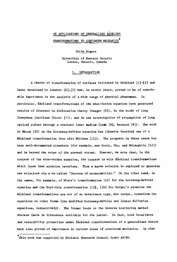
ON APPLICATIONS OF GENERALIZED BACKLUND
TRANSFORMATIONS TO CONTINUUM MECHANICS
Colin Rogers
University of Western Ontario London, Ontario, Canada
I. INTRODUCTION
A theory of transformation of surfaces initiated by Backluhd [1]-[3] and
later developed by Loewner [4],[5] has, in recent years, proved to be of remark-
able importance in the analysis of a wide range of physical phenomena. In
particular, BEcklund transformations of the slne-Gordon equation have generated
results of interest in dislocation theory (Seeger [6]), in the study of long
Josephson junctions (Scott [7]), and in the investigation of propagation of long
optical pulses through a resonant laser medium (Lamb [8], Barnard [9]). The work
by Miura [I0] on the Korteweg-deVries equation has likewise involved use of a
Backlund transformation (see also Whitham [Ii]). The progress in these areas has
been well-documented elsewhere (for example, see Scott, Chu, and McLaughlin [12])
and is beyond the scope of the present survey. However, we note that, in the
context of the sine-Gordon equation, the concern is with Backlund transformations
which leave that equation invariant. Thus a known solution is employed to generate
new solutions via a so-called "theorem of permutability." On the other hand, in
the cases, for example, of Miura's transformation [i0] for the Korteweg-deVries
equation and the Hopf-Cole transformation [13], [14] for Burger's equation the
Backlund transformations are not of an invariance type, but rather, transform the
equations to other forms (the modified Korteweg-deVries and linear diffusion
equations, respectively). The former leads to the inverse scattering method
whereas there is literature available for the latter. In fact, both invariance
and reducibility properties under Backlund transformations of a generalized nature
have also proved of importance in various areas of continuum mechanics. In view
This work was supported by National Research Council Grant A8780.

107
of the extent of the work in recent years on this subject only a survey can be
presented here.
The invariance and reducibility of the governing equations of gasdynamics
and magnetogasdynamics under various transformations has been the subject of
numerous papers over the last ten years or so, notably by the Russian School. One
may cite the works of Nikol'skii [15], Tomilov [16], Movsesian [17], and Ustinov
[18], [19] in gasdynamics and Rykov [20] in magnetogasdynamics. It is noted that
Ustinov [19] has utilized invariant transformations to solve certain finite-
amplitude shock-wave propagation problems in tubes.
It was Haar [21] who, in connectlon with a variational problem, first
introduced the adjoint transformations which leave invariant (with the exception
of the equation of state) the governing equations of plane potential gasdynamics.
Later, Bateman [22] constructed other such invariant transformations, namely, the
reciprocal relations. The latter were used by Tsien [23] to approximate certain
subsonic adiabatic gas flows. Bateman [24] subsequently noted that both the
adJoint and reciprocal relations are B~cklund transformations. Reciprocal pro-
perties for steady gasdynamics were further discussed by Power and Smith [25], [26].
These invariant transformations together with Prim's Substitution Principle [27]
were placed in the context of a more general formulation of invariant transfor-
mations for rotational flow by Rogers [28] ; extensions to nondissipative magneto-
gasdynamics were presented in a recent paper by Rogers, Castell, and Kingston [29].
Reciprocal and adjoint-type invariant transformations for (E+l)-dimansional
spherically symmetric unsteady gasdynamics were established by Rogers [30], [31].
These multi-parameter invariance properties may be applied to generate new solu-
tions from existing solutions of the original system. Application may be made to
certain problems involving nonuniform shock-wave propagation (Castell and Rogers
[32]). It is interesting to note that whereas there is a significant amount of
Russian literature devoted to invariant transformations and their applications in
gasdynamics and magnetogasdynamics (see above) this seems to largely have escaped
the notice of workers elsewhere. Certainly the method of invariant transformations
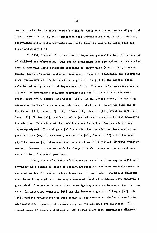
108
merits examination in order to see how far it can generate new results of physical
significance. Finally, it is mentioned that substitution principles in unsteady
gasdynamlcs and magnetogasdynamics are to be found in papers by Smith [33] and
Power and Rogers [34].
In 1950, Loewner [4] introduced an important generalization of the concept
of B~cklund transformation. This was in connection with the reduction to canonical
form of the well-known hodograph equations of gasdynamics (specifically, to the
Cauchy-Riemann, Tricomi, and wave equations in subsonic, transonic, and supersonic
flow, respectively). Such reduction is possible subject to the density-speed
relation adopting certain multl-parameter forms. The available parameters may be
employed to approximate real-gas behavior over various specified Mach-number
ranges (see Power, Rogers, and Osborn [35]). In the latter paper, the unifying
aspects of Loewner's work were noted; thus, reductions to canonical form due to
Von-K~rm~n [36], P~r~s [37], [38], Coburn [39], Frank'l [40], Kristianovich [41],
Sauer [42], Muller [43], and Dombrovskil [44] all emerge naturally from Loewner's
formulation. Extensions of the method are available both for certain aligned
magnetogasdynamic flows (Rogers [45]) and also for certain gas flows subject to
heat addition (RoSers, Kingston~ and Castell [46], Castell [47]). A subsequent
paper by Loewner [5] introduced the concept of an infinitesimal B~cklund transfor-
mation. However, to the writer's knowledge this theory has yet to be applied to
the solution of physical problems.
In fact, Loewner's finite Backlund-type transformations may be utilized to
advantage in a number of areas of current interest in continuum mechanics outside
those of gasdynamlcs and magnetogasdynamics. In particular, the Stokes-Beltrami
equations, being applicable to many classes of physical problems, have received a
great deal of attention from authors investigating their various aspects. One may
cite9 for instance, Welnstein [48] and the interesting work of Ranger [49]. In
[48], various applications to such topics as the torsion of shafts of revolution,
electrostatics (capacity of conductors), and virtual mass are discussed. In a
recent paper by Rogers and Kingston [50] it was shown that generalized Backlund

109
transformation may be applied to the Stokes-Beltrami equations with a view to the
generation of both invariance and reducibility properties. In a subsequent paper
by Clements and Rogers [51] it was shown that the well-known correspondence
principle of Weinstein emerges as a particular member of a multi-parameter class
of B~cklund-type transformation of the Stokes-Beltrami equations. Moreover, an
iterated form of the correspondence principle was used to obtain solutions to cer-
tain boundary-value probiems involving axially-symmetrlc deformations of an
incompressible isotropic linear elastic material. Such solutions assume importance
in light of recent work by Selvadurai and Spencer [52], where the first-order
theory serves as the basis for solutions in second-order incompressible finite
elasticity.
Reduction to canonical form of hodograph equations arising in fields other
than gasdynamics and magnetogasdynamics has also led to results of interest. In
this connection, Rogers and Clements [53] have shown that the hodograph equations
of one-dimensional elastic-plastic wave propagation in a medium which exhibits
strain-hardening behavior may be reduced to the classical wave equation subject
to the stress-strain relation in the plastic region adopting certain multi-parameter
forms. One of the latter has already proved useful for the explicit integration
of the elastic-plastic wave equations (Courant and Friedrichs [54]). The other
forms constructed in [50] may be utilized in a similar manner. An analogous
approach may he employed to analyze the propagation of large amplitude waves in
such media as saturated soil, dry sand, and clay silt. Thus, multi-parameter
stress-strain laws presented recently in an interesting paper by Cekirge and Varley
[55] (see also Kazakia and Varley [56]) may be generated via generalized Backlund
transformations. Moreover, further multl-para~eter forms are readily generated
via the method (Rogers [57]). Again, the parameters available may be used to
approximate real material behavior.
In the above classes of wave propagation problems, there are, of course,
the usual complications associated with discussions posed in terms of the hodograph
variables. However, for a variety of problems involving wave propagation through
110
various inhomogeneous media, significant progress can be made by use of generalized
B~cklund transformations to seek reduction to a convenient canonical form. Wave
propagation in homogeneous elastic media has been widely investigated. However,
studies involving wave propagation in inhomogeneous media are much less common;
a summary of the literature on this topic is given by Eason [58]. The problem of
uniform normal loading of the curved surface of a cylindrically or spherically
symmetric inhomogeneous elastic solid was introduced in a subsequent paper by
Eason [59] where the possibility of application in geophysical fields was noted.
Clements and Rogers [60], [61] have recently applied generalized Backlund trans-
formations to the study of wave propagation through elastic media with inhomo-
geneity. Specific boundary-value problems involving, for example, normal impact
loading of a spherical cavity were thereby solved.
The Backlund transformation approach may also be used to analyze long wave-
length pulse propagation in curved elastic rods (Moodle, Rogers, and Clements [62]-
where other methods are indicated) and in the study of (N+l)-dimensional
spherically symmetric shear waves in inhomogeneous isotropic viscoelastic media
(Rogers, Clements, and Moodle [63]). It is suggested that the exact solutions
generated thereby may be used to provide independent verification of the results
predicted by the Karal-Keller procedure for obtaining asymptotic wavefront
expansions for the travelling disturbance~ for example, resulting from dynamic
loading of hyperbolic-viscoelastlc materials. Again, similar cou~ents apply to
the analysis of certain wave propagation problems in flu/d-filled elastic tubes
(Rogers and Clements [64]). As a further application to B~cklund transformations
to problems involving wave propagation, we mention a recent paper by Clements
and Rogers [65] on two-dlmensional shallow-water wave generation over curved
bottom topographics both with and without ground motion. Current research is
being conducted on the application of Backlund transformations to the study of
radial propagation of rotary shear waves in an incompressible elastic material
under finite deformation employing as a basis, Blot's mechanics of incremental
deformations (Kurashige [66]).

111
Reduction to elliptic canonical form via BHcklund transformations has also
been recently used in nonlinear elasto-statics and other areas of continuum
mechanics. In the paper by Clem~nts and Rogers [67] application was made to the
theory of stress concentration for shear-strained prismatic materials with a non-
linear stress-straln law. Further, a broad class of nonlinear filtration problems
are amenable to the technique. Nonlinear filtration is of considerable practical
i~portance, since it arises, in particular, in connection with oil-drilling
operations. For example, flows of paraffin-based oils, of oils containing asphal-
tenes, and of oil-water emulsions are characterized by deviations from linearlty
in the law relating the rate of filtration and the pressure gradient. Rogers and
Swetits [68] constructed a variety of multi-parameter non-Darclan filtration laws
for which the hodograph system characterizing the nonlinear filtration is reducible
to a form associated with the Cauchy-Riemann equations. As an application of the
method, a wide class of nonlinear filtration problems involving a permeable medium
with cavities were solved. Finally, it is noted that finite B~cklund-type trans-
formations may be applied in the study of anti-plane crack problems in inhomo-
geneous elastic media (Clemants, Atkinson, and Rogers [69]).
In summary, it has been seen that the method of BHcklund-transformations
has widespread physical applications. Indeed, whereas an attempt has been made
to give an extensive llst of recent contributions, the list is by no means exhaus-
tive. It is the contention of the author that there remains much work to be done
in exploiting the technique to the fullest extent. The importance of the method
is two-fold. Thus, on the one hand, reduction to canonical form of wide classes
of physical problems may be made. The existing literature for the canonical form
may then be utilized to generate the solution of the original problem. On the
~ther hand, invariant properties may be constructed and employed to generate new
solutions from known solutions of nonlinear equations.

112
II. THEORY
Transformations
the type
~j § ~ , J = 1,2, U § U* characterized by relations of ,
(2.1) BI(~I,~2,U,U~I,U~2 -r* ~* U* U* U* , ~ 1 ' - 2 , , ~' ,~- " o ,
i = I,...,4 ,
_ ~U ~U* where U~j - ~j , U*~ -- 8~; were introduced by B~cklund in connection with
certain problems involving the transformation of surfaces. In particular, Backlund
transformations of pseudospherical surfaces which leave the total mean curvature
iuvarlant are discussed in Eisenhart [70]. These invariant transformations have
important applications in connection with the sine-Gordon equation mentioned
earller. A recent paper by Bauer and Rogers [71] was concerned with Backlund
transformations and infinitesimal deformation of surfaces.
In analogy with (2.1), generalized B~cklund-type transformations of the
form
(2.2) Bi(q'~2'Ul ..... ~'U1'q ..... ~'q'Ul'~2 ..... ~'~2;
~, r , U* U* U* . . . . . n ' ~ ,~ . . . . . ~ , ~ , u ~ , ~ . . . . . ~ , ~ ) = O , i,~2, i
i = i,...,2n+2 ,
may be introduced. It is assumed that all functions introduced have continuous
derivatives of all occurring orders. It is observed that if ~1' ~2 are regarded
as independent variables, and U 1 ..... %, U~ ..... Un* , ~, ~ are dependent
variables, the number of equations in (2.2) is the same as the number of unknowns,
namely, 2n+2. Resch [72] has investigated "linear" Backlund transformations
linking certain systems of partial differential equations involving an arbitrary
number of independent variables. Here, attention is confined to the case of
linear systems involving two independent variables. Even with these restrictions,
the transformations have widespread application. The applicatio n of generalized
113
BHoklund transformations to systems of nonlinear partial differential equations
remains to be studied.
The concern is with the application of certain transformations of the
type (2.2) to systems of n linear first-order partial differential equations
n
[=l[~i + 7ikUk ] + ~i = O, i = I, .... n , (2.3) k kUk' ~1 + 8ikUk' ~2
for the Uk(~j) , k = l,...,n, j = 1,2,. In (2.3), ~ik' 8ik' Yik are functions
only of the ~j. Specifically, if (2.3) is written in the matrix form
2 (2.4) j=l[ LjO~j + L3~ + L 4 = 0 ,
where L _= [~ik], L 2 -- [Sik], L 3 - [~ik], L 4 - [61 ..... ~n IT, and ~ -
[UI ..... %IT we investigate the subclass of generalized B'~cklund transformations
of type (2.2) defined by
(2.5)
R j ~ j + sj~z~j + z j~ + uj~* + vj = o , j = 1 , 2 ,
where 5, Sj, Tj, Uj are n x n matrices and Vj are n x i colunm vectors
with entries which are arbitrary functions of the 4" In view of the nonsingu-
larity conditions, IRj[ # 0, (2.5) may be rewritten in the form
~ = A j ~ j + B j~+ Cj6~ + Dj , j = 1,2,
(2.6)
~ = ~j ,
where Aj--RjlSj, Bj _---R3.1Tj, Cj--Rjluj, Dj--Rjlvj. It is observed that
(2.6) provides 2n+2 relations.
Transformations ~ § ~*, ~j § ~ defined by (2.6) are investigated which
transform the system (2.4) to an associated system
2 (2.7) ~ L~'~4"~ + L~*I~* + " =

114
where the L~ are functions of ~ - ~j.
Imposition of the cross-differentiation conditions
(2.9) ~,~, = ~** , , ~i~2 ~2~1
on the pair of matrix equations of (2.6) shows that
(2.10) (AI-A2)n~I~2 + (AI,~2-B2-C2AI)n~I + (BI-A2,~I+CIA2)~2
+ (BI,~2-B2,~I+ClB2-C2BI) + (C1,62-C2,61+CIC2-C2 C1 )~*
+ CID 2 - C2D 1 + DI,~2 - D2,~I = 0 .
Hence, if it is required that
A I ~ A 2 , C I , ~ 2 - C2,~1 + ClC 2 - C2C I = 0 ,
B 1 - A2 ,~ I + CIA 2 - ( A I , ~ 2 - B 2 - C 2 A I ) L I - I L 2 = 0 , IL l l # 0
( 2 . 1 1 )
(AI,~2-B2-C2AI)LI-~ 3 BI,~2 - B2,~I + CIB 2 - C2B 1 - = 0 ,
DI,~2 - D2,~I + CID 2 - C2D 1 - (AI,$2-B2-C2AI)LI-IL 4 = 0 ,
a matrix equation of the form (2.4) results. Further, from (2.7), it is seen that
2 (2.12) ~ L*~*., + L~* + L~ -
j=l j ~j
+ LI~IL~-I(L~D I + L~D2+L~)] + (L~Cl+L~C2+~)~*, IL~I # O ,

whence, if we set
(2.13)
115
L l l L 2 " - H , L~IL 3 " - J , LllL4 =-K ,
then provided
(2.14)
L -IL L =-H* , --J* L ffi-K* I ~ '
H = AIIH*A2 , IAII # 0 , J ~ AII(H*B2-BI)
J* = C 1 - H*C 2 ,
the matrix equation (2.12) yields
(2.15)
Thus, since A 1
K* ffi AIK + D 1 - H*D 2 ,
~* E1 - H*~2 - J*~* - K* = AI(fl~I-H~2-Jfl-K) �9
is nonslngular, it is Concluded that the system (2.4) is trans-
formed to the associated system (2.7) and conversely via the transformations
defined by (2.6). It is noted that if the ~i are isolated in the latter and
the requirement (2.8) is imposed, then no further restrictions arise, since only
the condition (2.10) again results.
The following result has therefore been established:
Theorem: The system
~i = H~2 + J~ + K ,
is transformed to the associated system
~ = H*~ + J*~* + K* ,
and conversely via th___~e ~eneralized Backlund-type transformations
ffi + Bj~ + Cj~* + Dj , ~ Aj~j
when the followln~ conditions hold:
(2.16)
w h e r e
116
B 1 -
C1,~2 - C 2 , ~ 1 + C I C 2 - C2C 1 = 0 ,
A2,~l + C1A 2 + ( ~ , ~ 2 - B 2 - C 2 A 1 ) H ffi 0 ,
BI,~2 - B2,~I
DI,~2 - D2,~I
+ CIB 2 - C2B 1 + ( ~ , ~ 2 - B 2 - C 2 A I ) J = 0 ,
+ C1D 2 - C2D 1 + ( ~ , ~ 2 - B 2 - C 2 A 1 ) K = 0 ,
A 1 = ~ , H " AI~*A 1 , IAll ~ 0 ,
(2.17) J - AII(H*B2-BI ) , J* - C 1 - H*C 2 ,
K* " AIK + D 1 - ii*D 2 �9
The above r e s u l t i n c l u d e s a s a p a r t i c u l a r c a s e (n ffi 2 , J = J* = K ffi K* ffi
D 1 = D 2 = O) t h a t o b t a i n e d by Loewner [4] ( s e e a l s o B e t s [ 7 3 ] ) i n c o n n e c t i o n w i t h
t h e r e d u c t i o n o f t h e h o d o g r a p h e q u a t i o n s o f g a s d y u a m / c s t o c a n o n i c a l f o rm i n
subsonic, transonic, and supersonic flow.
It is noted that any solution of (2.16) may be represented in the form
-i Cj = L~jL , J - 1,2,
is a nonsingular n • n matrix. Accordingly, if matrices A j , ~j, J~4'
(2.18)
where L
J = 1,2,
(2.19)
are introduced where
A3 = ~3 ' B3
t h e c o n d i t i o n s ( 2 . 1 1 ) r e d u c e t o c o n s i d e r a t i o n o f ( 2 . 1 8 ) t o g e t h e r w i t h
(2.20a)
(2.20b)
(2.20c)
117
~2,~ 1 - ~l,~2H - ~1 + ~2 H = 0 ,
~1,~2 , - ~2,~1 + (~1,~2-~2)J = 0 ,
51,~2 - 52,~1 + (~1,~2-~2)K = 0 .
In many physical contexts, the concern is with cases where J = J* = K =
K* = 0, whence, from (2.20b,c)~
(2.21) ~j = M~j , ~j - P~j , J = 1,2,
where M and P are arbitrary matrices. The matrix equation (2.20a) reduces to
(2.22) AI ,~I - ~l,~2H - M~I + M~2H = 0
which is linear in ~. A particular solution is
AI=M ,
whence, the general solution is
(2.23) ~l
where N i s the general so lu t i on of
(2.24)
Thus, the following result obtains:
Corollary: Th___%e
is transformad to the associated system
= M + N ,
- N~2H = 0 .
H~2 ,
and conversely by th_._~e generalized B~cklund-type transformations

118
~ = LCM+N)f~j + LM~j f] + L~jL-I~* + LP~j ,
~ = ~j , J - 1 , 2 ,
where L, M, N, and P are n x n matrices satisfying
H = [L(M+N)]-IH*[L(M+N)] , IL(m~)l ,' o ,
L~I H*L~2 (LM) ~1 = - = 0 , -H*(LM)~2 0 ,
- N~2H = 0 - H*P~2 - 0 . N~I ' P$1
IIl. REDUCTION TO _CANONICAL FORMS
Attention is henceforth confined to the class of transformations of the
theorem in the preceding section with the specializations n = 2, J = J* = K = K* =
Cj " Dj = O. Moreover, the matrices Aj, Bj are taken to depen d only on the
variable ~i" Hence, the results of the previous section show that
v i a the ma t r ix t r a n s f o r m a t i o n s
(3.2) - + , 2 ,
q + q , i - 1 , 2 ,
B 2 is a constant matrix and
(3.3) AI ,~ I - ".I*B 2 + B2AIIH*AI = 0 ,
In particular, in applications we are often concerned with systems with
where

13.9
(3.5) Hffi 2
h I
( 3 , 6 ) H * = , .
With these assumptions, it is necessary to specialize the matrix A I
property of zero diagonal elements is preserved under the mapping H ~ H*.
(3.4), it is clear that this property is invariant if (hut not only if)
the diagonal form
( 3 . 7 ) 'h . " a 2 '
so t ha t the
From
A adopts 1
in which case
( 3 . 8 )
while (3.3) yields
(3.9)
where
0 i~I, 2 aln2/a2
H* = A , ~ "l = . I . . k
2.2,1 a2nl/a I 0
i .I*.2 + .2".1. i. 2. 0 al,~l - n 2 b I n I o2Lal/a 2) = ,
.i*,2. 2. I. 2 .2". 1 + n2 Dl~a21al) = 0 a2,~l - n I D 2
Combination of (3 .9)a
(3.1l)
and (3.9)b shows tha t
1 2 det A 1 - ala 2 - constant - ~ ~ 0 ,

120
whence the system may be reduced to a single Riccati equation in either
2 a 2. In particular, the Riccati equation in al 1 is
1 1 2 2* 1 .2.1" (3.12) al,~l + e(a I) + 8 = 0 , where u = h I b2/A, 8 = -bln 2 �9
1 a I or
Loewner introduced the above class of transformations with a view to the
reduction to canonical form of the hodograph equations of gasdynamlcs for various
multi-parameter speed-denslty relations. The hodograph equations were placed in
the matrix form ~1 = KQ~2 and reduction to canonical forms associated with the
Cauchy-ltlemann, Tricomi, and wave equations was sought for subsonic, transonic,
and supersonic flow, respectively,
forma
(3.13)
Thus, H* was taken to adopt, in turn, the
Hence, specifically for the elliptic and hyperbolic cases (3.13) a
(3.14)
(a) (b) If 8 = 0 , If e = 0 , then
1 a I = 1 / (~1+e) . a~ = -B~I + ~ "
(c) ca) If 8/S > 0 , then
a~=(8/~)�89189 .
and (3 .13)c :
If 8/~ < 0 , then
a~=(-81~)�89189 .
In fact, as may be seen by consulting the references cited earlier, these reduc-
tions to canonical form and their extensions have applications in many areas of
continuum machanlcs outside Easdynamlcs. Two specific illustrations are outlined
in Section V.

121
IV. ITERATION AND THE STOKES-BELTRAMI EQUATIONS
Consider the matrix transformations
(4.1)
wl th
~ = q~q + BI~ ,
~ ffi A2~2 + B2~ ,
~= gj , j = 1 ,2 ,
= [Ul,U2 ]T ~* = [U~,U~] T
0 qp-1 ] (4.2) A1 ffi A2 = _~p+l 0 '
[0 :] [.701 (4.3) B 1 = (p+l) ~ ' B2 = 0
These transformations llnk the Stokes-Beltrami system
(4.4) ffi , I-I ffi , ~ 1 ~ 2 ~p+2 0
with the associated system
[ 1 o -ti p (4.5) ~ ~ ~*~, .~~ ~ o
Explicitly, these transformations yield
U~,~I = ~IP-Iu2,~I , U~,~2 ffi ~IP-Iu2,$2 -(P+I)U 1
(4.6)
p+l ~ = -q u I �9
The latter relati~ is Weinsteln's correspondence principle
(4.7) U2{ p} ffi C~+IuI{ p+2}

122
with C = -I. Iteration may be used to solve certain boundary-value problems
involving axially symmetric deformation due to solid inclusions in certain
rubber-like materials (Clements and Rogers [51]). It is readily established
by iteration of the above transformation that the general solution of the system
(4.5) for p - 2N, N = 0,i,... is given by
( 4 . 8 ) U~ + i~12Ntl~ -
(. A(~l'~2) ' 2N-r
~r where #(r)(~) 5 ~ {#(~)},
~ ~I + i~2 and ~(r)(o
N (-l)r2r(2N-r) I~ -2N+r (r)
[ rZ(S-r) z ~ (2H-r) - r = O
" t _ ~ ~(r)(O
d e f d a f N - r = 1 , 2N-r = 0 ,
when r = N = 0 )
~(~) b e i n g an arbitrary analytic function of
the complex conjugate of ~(r)(~) .
Further, the transformation
( 4 . 9 ) t t u~§ ,u~§ 1,~jff i~,
t a k e s t h e matrix s y s t e m (4.5) to
(4.1o) ~t t Ht~t ~ , ~t t t T %1 = " [UI'U2]
where
(4. ll) [ 0 [ ~i p o
Hence , t h e s o l u t i o n o f t h e S t o k e s - B e l t r a m i s y s t e m d e f i n e d by (4 .10 ) and ( 4 . I 1 )
with p = 2N, N = 0,i,... is given by

123
(4.12) U2t _ iU~ - A(~I,~2)
In a similar fashion it may be shown that the general solution of the
hyperbolic system
(4.13) ~ 1 2
for p ffi 2N, N = 0,i,... is given by
N (-l)r2r(2N-r)l~12N+rr (4.14) U~ *
rffi0 rl(N-r) l(2N-r) [F(~2+~ 1) + (-1)rG(~2-~l) ]
(4.15)
f(~l,~2 ) ,
N (-i) r2r(2N-r) ! ~ IF (r+l) (~2+~1) - (-1)rG(r+l) (~2-~1) ]
r=0 r l (N-r) !
E g(~l,~2 ) ,
where F, G are arbitrary functions of ~2+~i and ~2-~I, respectively, while
~(r) (~) denotes the rth derivative of ~ with respect to its indicated argu-
ment ~. The case N = 0 provides the familiar d'Alembert solution, while the
solution for N = 1 has been employed by Clements and Rogers [60] to solve a
class of initial-value problems related to wave propagation through inhomogeneous
elastic media.
Again, a simple transformation
(4.16) ~ § , u ~ § ~ j * ~
shows that the solut ion of the system (4.13) for p = -2N, N ffi 0 , 1 , . . . i s given
by
(4.17) U~ = g(~1,~2 ) , U~ ffi f(~1,~2 ) ,

124
V. APPLICATION
As indicated in the Introduction, there is a wide variety of areas in
continuum mechanics where quite simple Backlund,type transformations may be of
value either in the generation of Invariance properties or in the reduction of
problems to canonical forms amenable to solution by classical techniques. In
soma cases the boundary conditions in the transformed problem may be considerably
complicated by the procedure. However this is by no means always the case (for
exa~mple, see [60]). In many cases, use is made of a hodograph transformation
before reduction is sought via Backlund transformations. There are then, in
general, the usual difficulties associated with boundary-value problems trans-
formed to the hodograph plane. In other cases no hodograph transformation is
necessary to achieve reduction. Examples of both kinds of situation are indicated
below.
i. Aligned Nondisslpatlve MaEnetogasdynamics
The governing equations of the steady flow of a thermally nonconducting
Prim gas of infinite electrical conductivity in the presence of a magnetic field
are (in rationalized MKS units)
( 5 . 1 ) u j O , j + p u j , j = 0 ,
( 5 . 2 ) p u j u i , j + H , i - ~ H j H i , j = 0 , i = 1 , 2 , 3 , ,
(5.3) Hj,j = 0 ,
(5.4) ui,jH j - Hi,ju j - Hiuj, j = 0 , i = 1,2,3
(5.5) u j [ S ( s ) ] , j = o ,
(5.6) p = P(p)S(s) ,
1 where H = p + ~ ~HjHj, ~ is the magnetic permeability (here assumed constant),
while u i and H i designate the rectangular Cartesian components of the velocity
and magnetic fields , respectively. Further, O, P, and s denote the gas density,

125
gas pressure, and specific entropy, respectively. It is assumed that there are
no external forces present. To (5.1)-(5.6) are adjoined appropriate boundary
conditions (for example, see Rogers and Kingston [74]). Thus, for instance, for
the super-Alfv~nic aligned conducting flow past cylindrical insulars for which
the present analysis is particularly straightforward, the discontinuity in the
tangential component of the magnetic field implies the existence of a surface
current in the fluid layer adjacent to the insulator (Grad [75], Stewartson [76]).
It is readily shown (lurev [77]) that the equations of homentropic, plane,
nondisslpative magnetogasdynamics with aligned velocity and magnetic fields may
be reduced, under the additional assumption of uniform stagnation enthalpy to the
gasdynamlc-type system
(5.7) u*0~j3 + p'u* = 0 , J,J
(5.8) o*u*u* + p*. = 0 , i = 1,2 j i,j ,i
where the variables u*, p*, p* are given by
p* -= ]I , q* - q(l-~k20) ,
(5.9) p* - p(l-~k2p) -I 1 - ~k2p # 0
q*e i0 --- u* + iv* , qe i@ - = u+iv
I and uj, u~, j = 1,2 are denoted in turn by u, v and
that the k occurring in the aligned condition
(5.10) H i = kpui,, i = 1,2 ,
is a constant.
Stream and potential functions ~ and
to
u* v* ] (5.11) Vn = V~
-p'v* p'u*
u*, v*. It is assumed
may now be introduced according
where

126
(5.12)
A hodograph system
= [:] Y
(5.13)
where
~q, = Af~ 8
(5.14) h,
P 0 (l-uk2p)2q
(5.15) 0 < [J(q*,8,x,y)[ < " ,
is now established in the usual manner; in (5.14), M is the local Mach number.
If we now set
(5.16) -JqoL 1 - ~Ik 2 , t = 8
(where the negative sign is taken for the interval of variation of q in which
dq*/ds < 0) and q0 is a reference speed, the system (5.13) reduces to (if s
and K I/2 are real)
(5.17)
whe re
(5.18)
and K(s)
(5.19)
is defined by
A* m
~s = A*Rt

127
If s and K 1"2 / are imaginary, the hodograph equations reduce to the hyperbolic
form
(5.20)
where
(5.21) A** =
and
x -I/2 0
(5.22) a = -is , X I/2 = -iK I/2
In sub-Alfv6nic regions (~k2p > i), it is seen that, if M > I, the
hodograph system is elliptic. If M < i, since (~k2p) -I = A 2 = q2/h2 where
b = (~/p)i/2 H is the Alfven speed it is seen that the system is elliptic in the
region
and hyperbolic in t h e region
2 2
~22+b I~2 <I a
2 2
In super-Alfv~nic regions (~k20 < 1), as in conventional gasdynamlcs, t h e hodo-
graph system is elliptic for M < i and hyperbolic for M > i.
It is observed that the elliptic and hyperbolic matrix equations (5.17),
(5.18) are in a form suitable for the application of matrix Backlund-type transfor-
mations and the results obtained earlier apply. In particular, if attention is
restricted to super-Alfv~nic subsonic flow and we introduce the simple Backlund
transformation
t :J I:] (5.23) = , S' = S, t' B t , 0
where c is a real nonzero constant, then the new hodograph matrix H' is given
by (A > 1, M < 1)

128
Hence, subject to
(5.24)
H' =
_c2K-i/2
K being approximated by an expression of the type
K % = c 4
the magnetogasdynamic system defined by (5.13), (5.14) is transformed via (5.23)
to the Cauchy-lt[emann equations
! i ~ ! = (5.25) ~s -~ ~s ~
It is readily shown that the approximated q, p, p corresponding to the
approximation (5.24) are given by
q% ffi d[cosech(s0-s)+~k2c-2sech(s0-s)] ,
-2 t c t~h(sO-s)
( 5 . 2 6 ) 0 = , l+~k2c-2tanh(s0-s)
% _c2d 2 l+~k2c-2tanh p - [ (s0-s)]coth(s0-s) +
+ pk2c-4d 2 -�89 + e ,
where c, d, e, and s 0 are constants available for approximation purposes.
The latter relation can be written as
= ~k2d2p %2 pk2c'4d 2 (5.27) p% -c4d2P t-1 + + + e ,
2(l_~k2pT)2 2
which is the approximated "equation of state" in the aligned magnetogasdynamlc
flow. In the limit K + 0 , the celebrated K~rm~n-Tslen approximation of no=-
conducting gasdynamlcs is recovered.
2. Wave Propagation in Inhomogeneous Elastic Media with (s Spherical symmetry
The appropriate equation of motion in the case of uniform normal loading
of an (g+l)-dimensional spherically symmetric surface (E = 0,1,2) is
129
b~ r 82 u (5.28) ~T + e(Or-Oo)r-i = p ---
St 2
while the stress-strain relations adopt the forms
8u (5.29) Or = ~ ~r + 6~ur-i ' ~ = ~ + 2~ ,
~u (5.30) O 8 ffi I ~r + (el+2~)ur -I , e = 1,2 .
The case E = 0 refers to longitudinal wave propagation in an inhomogeneous slab,
and ~ being the Lam~ "constants"; for longitudinal wave propagation in an
inhomogeneous rod, ~ = E where E is Young's modulus. In the latter context,
r denotes the spatial coordinate measured along the rod, o is the stress, and r
u is the longitudinal displacement. For e = i, the equation of motion (5.28)
is for an inhomegeneous elastic solid subjected to uniform normal leading over a
cylindrical surface; in that case, u is the radial displacement, and Or, O@
are the radial and circumferential stress components in the usual cylindrical
(r,@,z)-coordinates. The relations (5.29) and (5.30) correspond to conditions of
plane strain; p, ~, and ~ are assumed to be dependent on r alone. Finally,
for E = 2 the situation described corresponds to that of uniform normal loading
of a spherical surface so that the only nonzero displacement is the radial dis-
placement Jn the radial component u. Just as for the cases E = 0,1, the quan-
tities 0, ~, and ~ are taken to be dependent on the radial coordinate r
alone.
(5.31)
Combination of (5.28)-(5.30) provides an equation of motion in the form
~r 2 r Dr r 2 + ~ + -~- =P ~t 2
where the primed quantities refer to derivatives with respect to r. It is con-
venient to introduce a function w(r,t) so that the governing equation (5.31)
emerges as a consequence of the matrix system
(5.32) fir = l~t + Nfl ,
where

130
(s. 33)
~nd 5 2 ' r a n ' n11
of w
( 5 . 34 )
~ = , M= , N=
21
a r e dependen t on
produces (5.31) ylelds
If we set
r alone. The requirement that elimination
de t M = - p / ~ ,
~rEml2 = e x p { - f n l l d r } ,
~m12[an/m.,2}' = c{ 2 ~ ' - ( ~ / r ) ' } .
~ exp{-/nlldr}
the system (5.34) gives
(5.35) m12 = ~-Ir~0 , m21 = prr , nll = -0'/~ ,
while # satisfies the equation
(5.36) r-C~[rE~#'/~2] ' - E{(~/r)'-(2/r)~'} .
Introduction of the new independent variables
( 5 . 37 ) u* = Ou , w* = u ,
r e d u c e s t h e s y s t e m (5 .32 ) t o
(5.38)
If new independent variables
(5.39) r* -
the system (5.38) reduces to
[:]i [0o~ vl[:l r*, t* are now introduced accordlnE to
r (pi~)112 dR , t* = t ,
r 0

131
(5.40) = 1/2 '
r* t �9
where
(5.41) K = p~r2e~ -4 ,
Matrix B~cklund-type transformations may now be applied to the system
(5.40) in the usual manner and reduction achieved to a form assoclated with the
conventional wave equation for various multl-parameter forms for O and ~. The
constants available in the latter may be utilized to fit 0 and ~ to curves
giving their variation for various inhomogeneous elastic materials. Reference
may be made to the recent paper by Clements and Rogers [61] where application is
made to a specific problem involving the propagation of radially symmetric waves
from an (e+l)-dimensional spherical cavity in an infinite inhomogeneous medium.
Application of a correspondence principle allows extension of such results to the
dynamics of initially dead inhomogeneous viscoelastic media.
VI. CONCLUSION
A survey of applications of B~oklund-type transformations in continuum
mechanics has been presented and some of the recent developments noted. Current
work (Clements, Atkinso~, and Rogers [69], Rogers, Ceklrge, and Askar [78],
Clements and.Rogers [79]) indicates a link with the linear integral operator tech-
nique of Bergman [80]. Thus, the transformations are associated with cases when
the series expansions of the latter method terminate. However, in view of Its
straightforward nature, the value of the Backlund transformation approach remains.
REFERENCES
[i] A.V. BXCKLUND, Ueber Flachentransformationen, Math. Ann. 9 (1876), 297-320.
[2] , Zur theorle der partiellen Differentlalglelchung erster ordnung, Math. Ann. 1_/7 (1880), 285-328.
[3]. , Zur theorie der Fl~chentransformationen, Math. Ann i_99 (1882), 387-422.

132
[4]
[5]
[6]
[7]
[8]
[9]
[10]
[ii]
[12]
[13]
[14]
[15]
[16]
[17]
[18]
[19]
[ 2 0 ]
[21]
[22]
C. LOEWNER, A transformation theory of partial differential equations of gasdynamics, NACA Tech. Note 2065, 1950.
�9 Generation of solutions of systems of partial differential equations by composition of infinitesimal Baecklund transformations, J. Analyse Math. 2 (1952), 219-242.
A. SEEGER, Theorie der Gitterfehlstsllen, Handbuch der Physik ~, no. i, 383-665, Springer, Merlin, 1955.
A.C. SCOTT, Propagation of flux on a long Josephson tunnel Junction, Nuovo Cimento B 69 (1970), 241-261.
G.L. LAMB, JR., Analytical descriptions of ultrashort optical pulse propa- gation in a resonant medium, Rev. Modern Phys. 43 (1971), 99-124.
T.W. BARNARD, 2N~ Ultrashort light pulses, Phys. Rev. A ~ (1973), 373-376.
R.M. MIURA, Korteweg-deVries equation and generalizations. I. A remarkable explicit nonlinear transformation, J. Math. Phys. 9 (1968), 1202-1204.
G.B. WHITHAM, Linear and Nonlinear Waves, John Wiley and Sons, New York, N.Y., 1974.
A.C. SCOTT, F.Y.F. CHU, AND D.W. MCLAUGHLIN, The soliton: a new concept in applied science~ Proc. IEEE 61 (1973), 1443-1483.
E. HOPF, The partial differential equation u t + uu x Math. 3 (1950), 201-230.
= ~Uxx , Comm. Pure Appl.
J.D. COLE, On a quasi-linear parabolic equation occurring in aerodynamics, Quart. Appl. Math. 9 (1951), 225-236.
A.A. NIKOL'SKII, Invariant transformation of the equations of motion of an ideal monatomic gas and new classes of their exact solutions, Prikl. Mat. Meh. 27 (1963), 740-756.
E.D. TOMILOV, On the method of invariant transformations of the gasdynamlcs equations, Prikl. Mat. Meh. 29 (1965), 959-960.
L.A. MOVSESIAN, On an invariant transformation of equations of one- dimensional unsteady motion of an ideal compressible fluid, Prikl. Mat. Meh. 31 (1967), 137-141.
M.D. USTINOV, Transformation and some solutions of the equation of motion of an ideal gas, Izv. Akad. Nauk SSSR Set. Meh, Zidk. Gaza 3 (1966), 68-74.
., Ideal gas flow behind an infinite amplitude shock wave, Izv. Akad. Nauk SSSR Set. Meh. Zidk. Gala ~ (1967), 88-90.
V.A. RYKOV, On an exact solution of the equations of magnetogasdynamics of finite conductivity, Prikl. Mat. Meh. 29 (1965), 178-181.
A. HAAR, Uber adJungierte Variationsprobleme und adJungierte Extremalfl~chen, Math. Ann. 100 (1928), 481-502.
H. BATEMAN, The llft and drag functions for an elastic fluid in two- dimensional irrotational flow, Proc. Nat. Acad. Sci. U.S.A. 24 (1938), 246- 251.
[23] H.S. TSIEN, Two-dimensional subsonic flow of compressible fluids, J. Aero.

133
Sci. 6 (1939), 399-407.
[24] H. BATEMAN, The transformation of partial differential equations, Quart. Appl. Math. 1 (1943-44), 281-295.
[25] G. POWER AND P. SMITH, Application of a reciprocal property to subsonic flow, Appl. Scl. Res. A_~8 (1959), 386-392.
[26] , Reclprocal properties of plane gas flows, J. Math. Mech. i0 (1961), 349-361.
[27] R.C. PRIM, Steady rotational flow of ideal gases, J. Rat. Mech. Anal. (1952), 425-497.
[28] C. ROGERS, The construction of invariant transformations in plane rotational gasdynamics, Arch. Rational Mech. Anal. 47 (1972), 36-46.
[29] C. ROGERS, SfP. CASTELL, AND J.G. KINGSTON, On invarlance properties of conservation laws in non-dlssipative planar magneto-gasdynamics, J. M~canique 1__33 (1974), 343-354.
[30] C. ROGERS, Reciprocal relations in non-steady one-dlmenslonal gasdynamlcs, Z. Angew~ Math. Phys. 19 (1968), 58-63.
[31] , Invariant transformations in non-steady gasdynamics and magneto- gasdynamics, Z. Angew. Math. Phys. 20 (1969), 370-382.
[32] S.P. CASTELL AND C. ROGERS, Application of invariant transformations in one- dimenslonal non-steady gasdynamics, Quart. Appl. Math. 3_~2 (1974), 241-251.
[33] P. SMITH, An extension of the substitution principle to certain unsteady gas flows, Arch. Rational Mech. Anal. 1__5 (1964), 147-153.
[34] G. POWER AND C. ROGERS, Substitution principles in non-steady magneto- gasdynamics, Appl. Sci. Res. 21 (1969), 176-184.
[35] G. POWER, C. ROGERS, AND R.A. OSBORN, Baecklund and generalized Legendre transformations in gasdynamics, Z. Angew. Math. Mech. 4-9 (1969), 333-340.
[36] T. VON KARMAN, Compressibility effects in aerodynamics, J. Aero. Sci. (1941), 337-356.
[37] J. PERKS, Quelques transformations des Equations du mouvement d'un fluide compressible, Comptes Rendus Acad. Sciences Paris 219 (1944), 501-504.
[38] _ _ , Sur l'integratlon des Equations qul reglssent le mouvement d'un fluide compressible, Proc. 7th Int. Cong. Appl. Mech. 2 (1948), 382-387.
[39] N. COBURN, The l~rm~n-Tsien pressure-voluma relatlon in the two-dimensional supersonic flow of compressible fluids, Quart. Appl. Math. ~ (1945), 106-116.
[40] F.I. FRANKL', On Chaplygin's problem for mixed sub- and supersonic flows, Izv. Akad. Nauk. SSSR 9 (1945), 121-143.
[41] S.A. KHRISTIANOVICH, On supersonic gas flows, Trudy TSAGI No. 543, 1941.
[42] R. SAUER, Unterschallstromungen um Profile bel quadratlsch approximierter Adlabate, Bayer, Akad. Wiss. Math.-Natur. KI. S.-B. 9 (1951), 65-71.
[43] W. M~LLER, Gasstr~mungen bel quadratlsch angen~herter Adlabate. Diss, Th. Munchen, 1953.

134
[44]
[45]
[46]
[47]
[48]
[49]
[5o]
[51]
[52]
[53]
[54]
[55]
[56]
[57]
[58]
[59]
[60]
[61]
G.A. DOMBROVSKII, Approximation methods in the theory of plane adiabatic gas flow, Moscow, 1964.
C. ROGERS, Application of B~cklund transformations in aligned magneto- gasdynamics, Acta Physica Austriaca 31 (1970), 80-88.
C. ROGERS, J.G. KINGSTON, AND S.P. CASTELL, The reduction to canonical form of hodograph equations in elliptic diabatic flow, Acta Physica Austriaca 3_44 (1971), 242-250.
S.P. CASTELL, Approximate solutions and applications of hodograph equations in elliptic diabatic flow, Acta Physica Austriaca 37 (1973), 193-204.
A. WEINSTEIN, Generalised axially symmetric potential theory, Bull. Amer. Math. Soc. 59 (1953), 20-38.
K.B. RANGER, Some integral transformation formulae for the Stokes-Beltraml equations, J. Math. Mech. 12 (1963), 663-673.
C. ROGERS AND J.G. KINGSTON, Application of Baecklund transformations to the Stokes-Beltrami equations, J. Austral. Math. Soc. 15 (1973), 179-189.
D.L. CLIENTS AND C. ROGERS, On the application of a Baecklund transforma- tion to linear isotropic elasticity, J. Inst. Math. Appl. 14 (1974), 23-30.
A.P.S. SELVADURAI AND A.J.M. SPENCER, Second order elasticity with axial s3mm~etry - I General Theory, Internat. J. Engrg. Sci. 10 (1972), 97-114.
C. ROGERS AND D.L. CLEMENT$, On the reduction of the hodograph equations for one-dimensional elastic-plastlc wave propagation, Quart. Appl. Math. 32 (1975), 469-474.
R. CODq~&NT AND K.O. FRIEDRICHS, Supersonic Flow and Shock Waves, Interscience, New York, N.Y., 1948.
H.M. CEKIRGE AND E. VARLEY, Large amplitude waves in bounded media. I. Reflexion and transmission of large amplitude shockless pulses at an inter- face, Philos. Trans. Roy. Soc. London Set. A 273 (1973), 261-313.
J.Y. KAZAKIA AND E. VARLEY, Large amplitude waves in bounded media. If. The deformation of an impulsively loaded slab: the first reflexion; III. The deformation of an impulsively loaded slab: the second reflexion, Philos. Trans. Roy. Soc. London Set. A 277 (1974), 191-250.
C. ROGERS, Iterated Baecklund-type transformations and the propagation of disturbances in non-linear elastic materials, J. Math. Anal. Appl. 49 (1975), 638-648.
G. EASON, Wave propagation in inhomogeneous elastic media, Bull. Seism. Soc. Amer. 57 (1967), 1267-1277.
, Wave propagation in inhomogeneous elastic media; normal leading of spherical and cylindrical surfaces, App1. Sci. Res. 21 (1970), 467-477.
D.L. CL~X~ENTS AND C. ROGERS, On wave propagation in inhomogeneous elastic media, Internat. J. Solids and Structures 10 (1974), 661-669.
, Wave propagation in (N+l)-dimensional spher- ically symmetric inhomogeneous elastic media, Canad. J. Phys. 52 (1974), 1246-1252.

135
[62]
[63]
[64]
[65]
[66]
[67]
[68]
[69]
[70]
[7l]
[72]
[73]
[74]
[75]
[76]
[77]
[78]
[79]
[80]
T. BRYANT MOODIE, C. ROGERS, AND D.L. CLEMENTS, Large wave-length pulse propagation in curved elastic rods, to appear J. Acoustical Soc. Amer.
C. ROGERS, T. BEYAN~ MOODIE, AND D.L. CL~4ENTS, Les ondes de cisaillament sym~trle sph~rlque en (I+l)-dimanslons pour un materiel visco~laetlque
inhomog~ne et isotroplque, submitted for publication.
C. ROGERS AND D.L. CLEMENTS, Wave propagation in fluid filled elastic tubes, Acta. Mech. 22 (1975), 1-9.
D.L. CLEMENTS AND C. ROGERS, Analytic solution of the linearized shallow- water wave equations for certain continuous depth variations, to appear J. Austral. Math. Soc.
M. KURASHIGE, Radial propagation of rotary shear waves in a finitely deformed elastlc solid, Internat. J. Engrg. Scl. 12 (1974), 585-596.
D.L, CLEMENTS AND C. ROGERS, On the theory of stress concentration for shear strained prlsmatlcal bodies with a non-llnear stress-strain law, Mathematlka 22 (1975)~ 34-42.
C. ROGERS AND J. SWETITS, On a class of non-linear filtration laws, to appear Rheologica Acre.
D.L. CLEMENTS, C. ATKINSON, AND C. ROGERS, Antl-plane crack problems for an inhomogeneous elastic material, submitted for publication.
L.P. EISENKART, A Treatise on the Differential Geometry of Curves_and Surfaces, Dover Publications, New York, N.Y., 1960.
K.W. BAUER AND C. ROGERS, Zur inflnltesimalen Deformation yon Flachen, Mathematische-Statistiche Sektion ForschungszentrumGraz 31 (1975), 1-15.
D. RESCH, Some Baeckland Transformations of Partial Differential Equations of Second Order, Syracuse University Thesis, Syracuse, 1950.
L. BEES, Mathematical Aspects of Subsonic and Transoni~ Gasdynamles, Wiley, New York, N.Y., 1958.
C. ROGERS AND J.G. KINGSTON, Non-dissipative magnetohydrodynamic flows with magnetic and velocity field lines orthogonal geodesics on a normal con- gruence, SIAM J. Appl. Math. 26 (1974), 183~195.
H. GRAD, Reducible problems in magneto-fluld dynamic steady flows, Rev. Mod. Phys 32 (1950), 830-846.
K. STEWARTSON, The dispersion of the current on the surface of a highly conducting fluid, Proc. Cambridge Philos. Soc. 53 (1957), 774-775.
I.M. IOR'EV, On a solution to the equations of magneto-gasdynamics, J. Appl. Math. Mech. 24 (1960), 233-237.
C. ROGERS, H.M. CEKIRGE, AND A. ASKAR, Electromagnetic wave propagation in non-linear dielectric media, submitted for publication.
D.L. CLEMENTS AND C. ROGEP~S, On anti-plane contact problems involving an inhomogeneous half-space, submitted for publication.
S. BERGMAN, Integral Operators in the Theory of Linear Fartial DifferentSal Equations, Sprlnger-Verlag, New York, N.Y., 1968.

SOME OLD AND NEW TECHNIQUES FOR THE PRACTICAL
* USE OF EXTERIOR DIFFERENTIAL FORMS
Frank B. Estabrook
Jet Propulsion Laboratory California Institute of Technology
Pasadena, California 91103
Such the use of forms Peculiar in the realms of Space or Time: Such is the throne which Man for truth amid The paths of mutability hath built Secure, unshakens still; and whence he views In matter mouldering, structures, the pure
forms...
- - J . M. W. Turner
I. INTRODUCTION
Cartan's calculus of exterior differentlal forms [1] is a convenient
mathematical tool for systematically applying many otherwise disparate tech-
niques of differential analysis. In the notational guise of modern differen-
tial geometry and mapping theory, this calculus has been used for deriving
important global results for systems of ordinary differential equations; we
believe it is at least as useful for expressing local, differential relations,
and especlally for treating systems of partial differential equations [2], [3],
[4).
This is a brief s,mm, ry of the differential form techniques we have
developed and applied thus far. Using a convenient notation, we first s,--m-rize
the algebra and calculus of forms. Unfortunately, there are many variations of
notation and even of the words that go with the underlying concepts; we will try
to indicate some of these as we go along. We always assume everything suitably
compact, continuous, and differentlable, although it will be obvious that in
This paper presents the results of one phase of research carried out at the Jet Propulsion Laboratory, California Institute of Technology, under Contract No. NAS7-100, sponsored by the National Aeronautics and Space Administration.

137
many cases differential form expressions are immediately convertible to integral
results by the Stokes theorems, and then topics like allowable topologies and
Jump discontinuities could be discussed.
An n-dimensional differentiable manifold can be most simply introduced
as a Euclidean space with Cartesian coordinates x i, i = i, .... n. This structure
ensures satisfaction of all the local topological requirements for continuous
point sets, so that we may proceed with the usual analytical and differentiation
operations when dealing with sufficiently continuous functions of the x i. But
once the local point set topology has been defined, the particular variables
i x are not in any way taken as intrinsically preferred over any other set
related to them by smooth non-singular transformation, and no metric, or measure
of distance or interval, is necessarily given. In practice, the identification
and postulation of sufficiently smooth independent coordinates to define a
differentiable manifold is always done quite automatically in setting up a pro-
blem, when there is a clear physical model to consider.
So, let us consider an n-dimensional differentiable manifold spanned
by a set of scalar fields x i, i s l,...,n, each with a continuous range of
values. A function ~(x i) of those scalars is then geometrically represented as
the family of (n-l)-dimensional surfaces obtained by setting ~(x i) = constant.
The total differential or gradient of a function ~ is the prototype 1-form:
at each point x i the expression
= ~-~--dx i ~ r idx i d~ 3x i
(we will use throughout the s,,~tion convention for repeated indices) describes
the orientation of the (n-l)-surface through the point~ and the spacing I there of
successive members of the family, relative to the coordinate grid and scales set
fOr better, density in the "quotient" space whose points are the (n-l)-surfaces.

138
by the x i. By the same token, the total differential dx I describes the
coordinate family of (n-l)-surfaces x I = constant, dx 2 describes the family
2 x = constant, etc. Thus the field d~ is at each point a linear superposltion
of components on the basis forms dx i there. These define a linear vector space
i at each point x , known as the cotangent space. In traditional tensor notation,
d~ is described by the array of its components: ~,i = ''''' n " Note care-
fully then that d~ is a first order covariant tensor field; one should not
think of it as an infinitesimal. A general 1-form, say ~, is an arbitrary
superposltion on basis 1-forms at each point: ~ = fi(~)dx i. One may linear
think of a local, oriented, spaced set of surfaces (a "sandwich" structure) at
i each point of the x space; if these are to mesh from point to point to form a
global family of (n-1)-surfaces, there must exist a function ~ such that
= d~, i.e. we would have fi = ~,i "
A (two parameter) family of (n-2)-surfaces could be described by setting
~(x i) = constant, ~(x i) = constant, where ~ and ~ are functions leading to
linearly independent 1-forms d~ and d~ at each point x i. However, arbitrary
functions ~'(~,~),~'(~,~) would do as well for describing the orientation if
they lead to independent 1-forms that are linear combinations of d~ and d~
The essential algebraic content is expressed by the "exterior" product, written
d~Ad~, where A denotes the completely antisymmetrized tensor product. This
is a geometric object which describes at each point x i the orientation, and
spacing, of a family of (n-2)-surfaces. In tensor calculus this "2-form" d~Ad~
is described by its coordinate components, ~,i~,J - ~,j~,i" It is a completely
antisymmetric second order covariant tensor, say Tij (of an algebraically special
iJkE kind called "simple" or "monomial", since it satisfies TijTk~C = 0). A
general 2-form is an arbitrarily linear superpositlon on simple basis 2-forms:
fij(xk)dxiAdx j .
General p-forms, p = l,...,n, are similarly defined with components on
simple basis elements of lower dimensional surfaces, such as (for p = 3)
fiJkdXiAdxJAdx k , J etc. This last expression is unambiguous because the operation

139
of exterior product, A, is associative. All p-forms, p = l,...,n, at a point
constitute an associative algebra--the Grassmann algebra--on the cotangent space.
The algebra of forms is constructed from scalar fields, and the
"Eulerian" operation d that operates on them to generate 1-forms. It is
shown in all standard references how this differential operation d is further
applicable to forms of any order. In tensor or coordinate language, it generates
the "curl"--a completely antisymmetrized set of partial derivatives of the
components of a given form, readily shown to be the components of a form of the
next higher order. An important theorem is that applying d twice one gets zero
identically. A form is called "exact" if its exterior derivative is zero. The
�9 i "natural" basis forms dx I belonging to a coordinate frame x are obviously
exact.
We have to remember thus far the rules for manipulation:
~Ao = (-I)PqoA~ ,
d(~Ao) = do.~Aa + ( - l ) P u ~ d c ,
dd~=O ,
d c = O ,
where p and q are the orders of ~ and ~, respectively, and c is a
constant.
Although in tensor calculus 1-forms are called "covariant vectors", the
terminology should perhaps be avoided because (contravariant) vectors are very
different geometrical objects. (In Riemannian geometry one always has a way of
associating l-forms and vectors, using a metric tensor gij and its inverse
giJ.) On the other hand, the true vectors, which we consider next, do come close
to the concept of an (n-l)-form. The latter describes, at a point, the orien-
tation and spacing of a family--or congruence--of 1-dimensional submanifolds. By
"spacing" is meant the density of the points representing the submanifolds in
the (n-l)-dimensional "quotient space" of the congruence. If a density field in

140
n-space were also given, 2 the (n-l)-form, divided by this, would describe the
orientation of a congruence together with a magnitude which now is a measure of
1-dimensional extension or length at each point, and this, up to a simple choice
of sense or direction, i_~s the geometric description of a vector field,
Ill. VECTORS
A family of 1-dimensional submanifolds, "calibrated" with an internal
coordinate laid out along their lengths, is a vector field ~. In any coordinate
i d system x one has (in an older notation where by ~ one means "total"
differentiation) a set of autonomous flrst-order ordinary differential equations
dx i d~--= vi(~) '
and the general integral of these is a parametric description of the submanifolds:
i i x = H (s,al,a2,... ,an_l). The dependence on the scalar field s fixes the
internal calibration. In a notation to be introduced shortly, we would have
~-ds = i. al,... ,an_ 1 are n-i (the maximum number) independent "constants
of the motion", or "first integrals" or "co-moving coordinates"; ~.da i = 0.
Any n-i ~dependent functions of the a i would do as well. Moreover, s could
be "set" differently on each line of the congruence, without altering the ~,
by writing x i = Hi(s ' - P(al,... ,an_l) ,a I ..... an_l ) = Hi(s' ,a I,. .. ,an_ l ) �9 Thus
the fanctional form of the H i is far from anique. We will see how a unique or
canonical functional description of the congruence of 1-dimensional submanifolds
-i can be set up using n constants of the motion, say x , chosen so that
i -i x = x at s = 0. s is then treated as an external parameter, each fixed
value of which corresponds to a point translation or mapping of the entire space
i -i along the congruence: x § x .
The functions V i in the above set of equations are denoted "components"
of ~ with respect to the x i. In the sense that this is a set of directional
2For example, by the single non-vanishing coordinate component of an n-form, or by
just the single quantity ~d/~et gijl calculated from a metric tensor field.

141
derivatives of the x i, along ~, these equations are best written as a set of
Lie derlvatlves--we will return to that interpretation of a vector field shortly.
There is, however, a local sense in which ~ gives an entity in an n-dimensional
linear vector space attached to each point of the diffarentlable manifold. This
is the tangent space~ the objects (vectors) in which turn out to be algebraically
dual to the objects (1-forms) in the cotangent space there. That is to say~ we
will find an operation of inner product or contraction between them: at a point,
any vector ~ maps all 1-forms onto the real numbers (or conversely).
All vector fields ~ which have the same components ~ at a point
i x i ( s o '" x 0 = ..) are, as an equivalence class, denoted (without changing the
symbolism) just the vector ~ there. We can arrange that s o = 0 there for all
of them. They are all mutually tangent~ and in particular tangent tO a family of
i 1-dimenslonal manifolds that is linear--straight--with respect to the x
coordinates~ so satisfying
i i dx i s i ~ (XJo) s x ~x0+ ~x0+ ds s=O
i Clearly~ any such local vectors at x 0 can be llnearly superimposed, as with any
fixed conventional value of s they are now seen as displacements in an afflne
space--agaln the tangent space. This construction provides the usual geometric
image one has of vectors as superlmposable displacements to neighboring points, but
in the dlfferentiable manifold itself this is only strictly true for infinitesimal
values of s (unless one restricts oneself to a particular coordinate frame and
those linearly related to it--agaln the afflne geometryl).
Any coordinate frame x i, which furnishes basis forms dx i for the
cotangent space~ also furnishes dual basis vectors for the tangent space. We
denote by ~i the 1-dimensional submanifolds on which 2 x 3 n ... �9 x are
1 constant~ and on which we adopt a calibration so that x s s. The rest of the
~i are similarly defined. Any vector ~ then is expressed in the basis
belonging to the coordinate system as viii , where the ~ are as before the
components with respect to that same coordinate system.

142
i At a point, say x0, dx I describes the orientation of an (n-l)-
1 1 surface through the point, on which x = ~ is constant, and describes as well
t_he spacing of adjacent surfaces of the same family. Laying off an infinitesimal
e~ i from the point we stay in the surface if i # i, and we displacement are
surface if i = I. The calibration of ~I ensures that b r o u g h t t o an adjacent
1 1 in the last case the value of x on the adjacent surface is just x 0 + s The
change in value of x I along any vector is a scalar denoted the inner product,
or contraction, of the vector and dxl; it is denoted by an interposed �9 or
J For r we have Just found s = s in general we have
- .
We then find V i = ~.dx i and (vi~i).(fjd~) = vifl. Both forms and vectors
enter the contraction operation linearly.
One Justifies, and remembers, the following general rules for contrac-
tion of a vector with higher rank forms :
<~ + ~.~ = ~.~ + ~.~ ,
(f "~ = fV'~ ,
~~ = (~.~)Ao + (-1)P~A(~'O).,
where p is the rank of ~.
In modern texts vectors are defined in a different fashion. A vector
field is the generator of a 1-parameter continuous group of transformations of
the space, a dlffeomorphlsm mapping it onto itself. More explicitly, the functions
~(~) can be regarded as generating a 1-parameter family of scalar fields
xi(~,s), of which xi(x]'O) = xl' ~s s=O " vi' and the hlgher-order Taylor
series coefficients are determined from these by the group property. A symbolic
expression of this transformation group is
~i . dCxJ,s> = exp<s~> i ,

143
which implies the transitive rule
Fi(~ (~ , s ) ,~) - Fi(~,s+;) .
The inversion is x i = Fi(xJ,-s). In x i space the x i are n first integrals
of Vi(x j) �9 and this relation is a canonical functional description of the
congruence of calibrated lines. By imposing one arbitrary functional relation
between the x i, for each value of the parameter s we would find an (n-1)-
i manifold in the space of the x , and so s Would then again appear as a scalar
field there in an internal parametric description.
i s is a linear differential operator which, when applied to x , gives
the set of scalars vi; this follows from the above, or simply from calculating
-i i s x i ~ llm x - x ~ . f s - ~ s
We ignore all global and topological niceties of the modern understanding
of diffeomorphisms of differentiable manifolds, and simply assert that (in most
neighborhoods) the linear operators ~ on a differential manifold are abstractly u
equivalent to the vector fields ~ as we previously introduced them~ they have
the same coordinate components, the scalar fields ~ x i = V i = ~'dx i. Since any V
scalar ~ could be a "coordinate", we have in fact
~= ~.d~ V
A continuous group of mappings of a differentlable manifold onto itself
maps at the same time all geometric objects in it. Thus ~ can operate on V
scalars, forms, and vectors. The result is in each case necessarily of the
same tensor character, and is called the Lie derivative with respect to V.
Applied to scalars, it has been seen to be the usual substantial or
material derivative of fluid mechanics. (We previously described 1-forms as
"Eulerian"; we can now make the dual remark that vectors are "Lagrangian.") The
directional or Lie derivative of forms, or other tensors, is less familiar than
it should be, as it provides a very useful way of understanding, and remembering,

144
the otherwise somewhat mysterious "correction terms due to the change of reference
frame" that arise in all Lagrangian formulations for tensor fields. The key
property of s is that it is a derivation operator obeying Leibniz v rule.
While we have not shown all this in detail here, the needed formulae for
practical manipulations can now be quickly obtained. ~
First, for exact forms dx i, since dx i = dx i + sdV i + ...,
~ l x i ffi l i m - - d x i - d x i ffi d ~ = d+s i s+O s V
For a general 1-form ~ = fidx i we then have
= ( ' s + fl +s ~ ~ v
= ( ~ . d f i ) d x i + f i d ~
§ i i = ~.d~ + (V.dx)fi + d(fiV ) - Vidfi
= ~ ' d ~ + d ( ~ ' ~ ) ,
and in fact this last relation holds for any form ~, of any higher rank. If
is exact, say du, it says that ~s and d are always co~uting operations: V
s d (~ .d~) = § + = = d ( V . d ~ d ( ~ . ~ } ) d ~ .
The Lie derivative of one vector field W with respect to another
can be found most readily in terms of components:
~-d~ = ~ = ~C~'d~i> = C ~ > ' d x i + ~ '~dx i = %~>i + ~ . d ~ v V V V V
o r
c ~ > i . ~.dWi _ ~.dV i . V
This is antisy~metric in the two vectors. It is customary to denote it as the
Lie product, or bracket or commutator, [V,W], which is quite appropriate since
we hera regard the vector fields as linear operators. This also provides a
language for geometrically expressing the properties of Lie groups and algebras.

145
As for "natural" basis vectors ~i (i.e. derived from coordinates), they
satisfy [~i,~j]__ = 0. A co,non "operator" notation for the basis vectors is
~. = ~ / ~ i . i
One finally needs to remember only four results: that ~ is a
V derivation both for forms
V V V
and for contractions
g(~.~) = [~,~1.~ + ~ . ~ , v
that the Jacobi identity holds for vectors,
[ ~ , [ 0 , ~ ] ] + [ ~ , [ ~ , ~ ] ] + [ ~ , [ ~ , ~ : ] ] = o,
and that, operating on any geometric object,
_~/ = s
IV. INTEGRATION
A p-form ~ can be integrated over a p-dimensional subspace V. A
commuting set of p independent vector fields lyinE i__nn V (hence said to be
p-forming), say VID...,Vp, can be used to divide up the subspace into infini-
§ p~p,3 tesimal p-par-lleloplpeds with edges ~iPl ,. . .,~ and for each of these the
form ~ can be evaluated by contraction: el...r (...( .~)...)). An
integral is then defined by snm"~ng all these to the (p-1)-dimensional bounding
manifold (denoted ~V), and suitably going to a limit. The symbol for this is
/V ~ as (due to the antlsyuenetry of the p-form) the result is independent just
of the auxiliary mesh.
The generalized Stokes theorem can be proved by laboriously considering
3Thus we a r e a s s u m i n g f o r c o n v e n i e n c e and b r e v i t y t h a t V i s " o r i e n t e d " .

146
the integration just described.
simple (orientable)
where o is a (p-l)-form, and
so do = 0, we have I~V O = O:
manifold is zero.
One need only remember that if the topology is
do is an exact p-form. If o is exact, in
the integral of an exact form over a closed
V,
It may be shown--indeed, is an alternate way of defining Lie derivatives
of forms [4]--that if the points of the integration boundary ~V are infinitesi-
mally displaced by E~ the change in /V $ is ~/V ~ ~" This is a very useful w
rule for variational calculations.
V. THE SOLUTIONS OF PARTIAL DIFFERENTIAL EQUATIONS
AND THE INTEGRAL MANIFOLDS OF IDEALS OF FOP~
An immersed manifold or subspace V of p-dimensions can be described P
by giving n - p variables as f=nctions of p others: this is the geometrical
distinction between dependent and independent variables. We will in this section
define the so-called integral manifolds V belonging to--defined by--a given P
set of exterior differential forms. These are solutions of resulting sets of
first-order partial differential equations, and it follows that the many
systematic techniques for manipulating differential forms consequently have
much practical use in the analysis of sets of partial differential equations.
In the next section we will consider the construction of the so-called "regular"
integral manifolds, which is Cartan's generalization of the Cauchy-Kowalewski
theorem to sets of first-order partial differential equations. We will come
upon criteria for a set of forms to be '~ell set", viz. that its regular
integral manifolds include almost all of the usually required solutions of a
given set of partial differential equations. (The exceptions are so-called
"singular" integral manlfolds describing certain characteristic or exceptional
solutions; on the other hand, the regular integral manifolds can include

147
generalized solutions introduced by Lie in which the roles of some independent
and dependent variables are interchanged.) Such considerations may eventually
lead to sharper criteria than we can at present formulate for the proper choice
of sets of forms to represent partial differential equations.
Consider as an example that we are given, in n-space, a set of m < n
A independent 1-forms ~ , A ffi l,...,m, together with their exterior derivatives,
the 2-forms d~ A. (For simplicity we do not explicitly consider any other 2-
forms, independent 3-forms or higher, to be given, but it should be clear, how
readily they could be included.) Denote this a Pfaffian system. If we find a
set of independent vector fields 71,. ,~ all of which lie in a family of �9 " p'
p-dimensional subspaces Vp (this requires [~i '~J ] k~-> = fi~Vk and is denoted
p-forming 4) , and which are such that they each annul (give zero when contracted
A on) any
+ A V i.~ = 0
then by operating with s it is quickly found that also v j
�9 + + A
v i . v j . d ~ = o .
Any vector in V annuls any 1-form in the set, and taken two by two, any pair P
of vectors annul the 2-forms d~ A. Such a Vp--Containing --is called
an integral manifold, or integral subspace, of the set A, d A. Our definition
is easily extended to sets including forms of higher rank; again their exterior
derivatives can be included. Any set is denoted "closed" if it includes the
exterior derivatives of all forms in it, and we will henceforth only consider
closed sets. In general they will have integral manifolds of various dimension-
alities p = 1,2, ....
In modern texts a subspace V is described as a map ~ taking P
points of the p-manifold V to the immersing n-manifold (n > p). Forms-- P
4By k + rescaling the ~j the fij _ could he made zero--the Vj would then form a
mesh of p-parallelopipeds like the ~j of a coordinate frame in Vp.

148
themselves locally described as arrays of components on subspaces--are readily
* A d~A shown to transform only under the inverse map ~ , i.e. forms ~ and
in the n-manifold may be "pulled back" (or mapped, or induced, or sectioned) by
unto V where they may be denoted ~A and d~A 5 They are there p*
expressible solely in terms of a p-dimensional basis of 1-forms. In the present
case, since the results of contracting m A with any vector in V and d~ A P
with any pair of vectors in ~ are both zero, the condition determining P
integral submanlfolds can be restated simply as ~A = 0 and c~ A " 0. ~o
finally, for a general set of forms, of no matter what rank, an integral mani-
fold is defined by requiring them all to be zero when pulled back into it. Since
d and the inverse mapping opera=ion ~* commute~ the sets of forms considered
may always be taken closed.
Since the forms A d A, etc. only enter the definition of intsgrable
manifolds through linear homogeneous equations, it is clear that any algebraically
equivalent set o f formS mey be used. It should, in fact, perhaps have been
stated at the on=set tha~ it is an entire ideal of the cotangent space Grassm~n~
algebra, generated by the given forms, he, re A and d~ A, that is annulled--
pulled back to vanish in any integral ,~nifold V. That is to say, all 1-forms
such as fA~ A. 2-forms ~AAm A + fAd~ A. etc. (fA being arbitrary functions,
~A being arbitrary 1-forms, etc.) will obviously be annulled, when ~A and
dw A are. For a Pfafflan system any set of n - m linearly independent 1-forms
A algebraically formed from the ~ , together with its closure 2-forms, generates
BA the same ideal: fA ~ , d(f u~ A) , where ~he functions are such that
If]l § 0
If we introduce p autonomous independent variables y~, ~ = I,... ,p
as a basis in every ~, we have. if A = ~ i A ( ~ ) d x i , dtoA = ~i,jdxA JAdxi, that
~A A ~x i d~A A ~ ~x i " ~i -- dye' ffi ~i,J dy ~ A dy ~. Setting these equal to zero, term
~y~ ~y~ ~y~
by term, gives a coupled set of partial differential equations for n dependent
5For any p-form ~ it follows that IV ~ " IV ~ " p p

149
variables x i as functions of the y~. Any algebraically equivalent set of
forms, pulled back to zero, will give an equivalent coupled set. If p of the
i x can still vary freely in the integral manifolds, they could have been
adopted as the independent variables and non-autonomous equations would result
for n - p dependent variables. In either event, note that all integrability
conditions are explicitly included in the resulting set of first-order partial
differential equations.
VI. THE REGULAR INTEGRAL MANIFOLDS AND CARTAN'S CHARACTERS
We are often asked about the converse problem: given a set of first-
order partial differential equations~ how to choose a set of forms,to represent
the desired solutions. Cartanls generalization of the Cauchy-Kowalewski theory
gives criteria guiding this selection. The selection is even then far from
unique; nevertheless we have found in practice that all such sets of forms are
highly useful. We suspect that more succinct criteria will emerge after further
experience.
Cartan considers a sequence of families of successively higher-
dimensioned integral manifolds denoted, from their sequential construction from
boundary conditions~ as "regular". Algebraic criteria emerge for the "degrees of
freedom" in the construction of the regular integral manifolds, in terms of so-
called "characters", obtained from the ranks of certain sets of linear algebraic
equations. In the maximum dimensional family (which has the maximum number of
independent variables), those variables which can still be freely varied are
denoted as being "in involution" (this termioology is not to be confused with
that of Hamiltonian theory). We consider a set of forms to be '~ell set" for
describing a given set of first-order partial differential equations, when the
maximal regular integral manifolds of the set of forms are the desired solutions
of the equations, and the given independent variables are in involution. These
criteria can be determined by purely local arithmetic calculations with the
characters.

150
Begin, at some general point having coordinates
chosen such that the m conditions
X , with a vector 1
§ A Vl.m = 0
are satisfied. These are a set of homogeneous linear algebraic equations
i + i § relating the n components V 1 = Vl.dX of V I. To conform with Cartan's
notation, denote the rank of this first algebraic set that we must consider by
(=m), so ~i = n - s o > 0 components of ~i may be chosen arbitrarily. s o
i i (We take this rank to be at its maximum at x , and in a neighborhood of x .
Thus we ignore all special cases that might arise in this and the following,
for clarity of exposition of the central ideas.)
We can now advance to the point ~i = x i + eV~ where 6 is infini-
tesimal, and again make ~I choices (which can differ from those first made to
-i order e) to determine a vector ~i at x . This can be done in repeated
i fashion, varying the V 1 each time to the same order c, so by a limiting
process based on the sequence of such step-by-step choices we construct a
continuously imbedded 1-dimenslonal integral manifold V 1 = { x i : x i = f i ( s ) ,
dfi/ds = V~(s)}. In constructing such a V I we have made ~i choices of
functions of one variable while integrating a set of ordinary differential
equations from given initial conditions.
point of a V I we can choose a vector ~~ At each such that
.mA = 0 ,
V2.Vl.d~ = 0
(If there were other 2-forms given, in addition to the d~ A, we would include
them also in the last equation.) The rank of this set of homogeneous linear
equations for the n components of V 2 is not less than So, we denote it,
with tartan, s o + s I. So we can in general choose %2 = n - (s0+s I) members
i arbitrarily. We remaxk, however, that the set ~i is of of the set V 2

151
course a solution of the above equations, and so is included in the ~2 linearly
independent possible choices. If it were the only possible choice, we would
not be able to proceed with the construction of a V 2, so let us assume
s > i.
i We can now, from each point x of Vl, advance to a neighboring
point x i + ~V~ not in V I. ~ is again infinitesimal. A new, neighboring
V 1 is thus constructed point-wise; it will have a natural calibration carried
along from the c steps on the first VI, i.e. a new V 1 is given at each
point. We will show in a moment that this new V1 is again an intesral mani-
+ A fold, i.e. that still VI-~ = 0.
of freedom, can be made on the new
construction now steps along in
A varied choice of V2, within ~2 degrees
VI, and indeed on each new V 1 as the
intervals. Again by a limiting argument
�9 . ~fi i we.assert that a V 2 is thus constructed: V 2 = {xl:x I = fi(s,t), ~-~-= Vl(S,t),
~fl i ~t = V2(s,t)}~ We have now made 12 further choices of funetions~ this time
functions of two variables.
+ V 1 has not been free in this last construction, rather it has been
defined at each step so as to be "carried along" V2, forming infinitesimal
parallelograms that close. That is, we have determined V I throughout V 2
by the condition [VI,V2] = 0. This is also clearly the integrability require-
ment on fi(s,t). Its imposition is the key to Cartan's construction. For
+ A consider the resulting scalar fields VI.~ in V 2. The Lie derivatives of
+ + A + ~ .A § § A + A these along V 2 are i (VI'~) = [V2'V I] + VI'{d(V2"~ ) + V2"d~ }; but
V2 § A these are zero, term by term. Thus since Vl.m = 0 on the "boundary"--the
initial Vl--they remain zero throughout V 2. Thus we have indeed constructed
V 2 so that any vectors in it, contracted on the A, give zero, and so that
any pair contracted on the d~ A gives zero. It is an integral manifold. I
The construction continues. Given a V2~ choose at each point a V 3
such that

152
§ A V3"d~ = 0 P
"+ § A V3"Vl'd~ = 0 |
§ § A V3"V2"d~ = 0 .
(If there were independent 3-forms in the given closed ideal of forms, obviously
i the required additional linear homogeneous equations for V 3 would be included.)
i In calculating the rank of this linear homogeneous set for the V 3 one must
take account of all information known about the coefficients, e.g. that
§ § A VI'V2"d~ = 0, etc. The algebraic rank is denoted So + Sl + s2; ~3 = n -
(s o + s I + s2) independent solutions can be arbitrarily chosen. If E 3 > 2, a
V 3 can be constructed by making E3 choices of functions of 3 variables; V 1
and ~2 are constructed at the same time throughout the V 3 such that
t'1,* 1 - o , " o, t 1, 23 - o , and i s sho to be an i n t e g r a l
manifold. The proof at each stage depends essentially on the fact that the
ideal is closed.
The positive integers So, Sl, s2,.., are denoted the characters. They
are numerical invarlants of the ideal of forms. Since we have %p < ~p-l'
p - 1,2,..., and moreover require at each step ~p > p - i, the sequential
construction must terminate: there must be a maximum dimension of the families
of regular integral manifolds. Let the largest value of p be denoted g, the
- . + S g _ l ) = genus; then ~g n - (s0+sl+.. > g - i, and ~g+l n - (s0+sl+...+
Sg-l+Sg) < g' ~g+l < h" If ~g > g, the integration scheme remains under-
determined at the last step: the equivalent set of partial differential equations
for n - g dependent variables and g independent variables will be under-
determined in that arbitrary functions of the independent variables will enter
the solution.
The case of most interest 18 when ~ = g: there is then no freedom in g
the last construction--V is determined by properly set data on its bouedary. g
In thls case the above inequalities require the precise relation

153
n - g = s0 + Sl + ... + Sg_l �9
This is an important diagnostic test for a closed ideal of forms to mset, to be
chosen to represent a proper set of partial differential equations: the sum of
the Caftan characters s o + s I + ... + Sg_l , where g is the number of indepen-
dent variables, must equal the number of dependent variables, n - g. Conversely,
it seems to us a criterion for a "proper" set of partial differential equations
that such an ideal can be found to represent it.
VII. INTEGRABLE SYSTEMS
If affine transformations of the 1-forms of a closed ideal can be found
which yield exact 1-forms (i.e. if there are exact 1-forms in the ideal) the
ideal is partially integrable. This case is concerned with the existence of
envelopin8 manifolds (which arise for Pfaffian systems when s I < So). They are
by considering any n - m independent vectors ~, ~ = i,... ,n-m, found which
given A: Consider any Lie product [~3,~o] ; if it is independent annul the of
the ~ , define it again to be a ~m' say. It will not annul the A, hut no
continue taking all possible Lie products of ~T's until closure is matter,
achieved. Denote the dimensionality of that family of manifolds to be n - q >
n - m. If q > 0D we have envelopment: the manifolds can be described by setting:
~i ~ constant,
Sq = constant,
and the exact (~) 1-forms d~l,...,d~ q are dual to all the ~T' and in particular
to the original ~:
But this is am saying that the exact forms
A
~ ' d ~ b = O, b ~ 1 . . . . , q , ~T = 1 , . . . , n - m .
d~ b m u s t b e i n t h e i d e a l o f t h e
154
de b fA Ah , b = 1, .... q, q < m .
b = The fA are integrating factors, and by putting the integrals ~b constant,
our original set of forms can be reduced to a set in n - q dimensions; the only
problem is to ascertain that we have found the maximum value of q, or the
minimum dimension of the enveloping manifolds.
An alternate approach to finding exact 1-forms in an ideal is Just to
consider the equations that result from expanding
dfA/~ A + f A ~ A ~ 0 .
These are an overdetermined set of linear partial differential equations for
fanctions fA(xi). If solutions exist, for each independent solution one can
find a ~ (up to arbitrary constant), d~ can be used, instead of one of the
"'A it depends on, as a basis for the ideal. The search for exact forms in a
given ideal can be very useful also for higher rank forms. We will discuss this
when we consider conservation laws.
For a Pfaffian system, in the extreme case when we find q = m, the
number of independent 1-forms, we would find all the d~ A in the ideal of just
the ~A--they contribute no independent equations to Cartan's constructions and
could be dropped, s o = m, s I = s 2 = ... = Sn_m = 0. This is called a
"completely integrable Pfaffian system." It could alternatively be described as
n - m vector fields--coupled ordinary differential equaKions without further
integrahility conditlons. 6 The maximum regular integral manifolds then are of
dimension g = n - m, and so are ~he minimum enveloping manifolds--they coin-
cide! In this way we have come upon the Frobenius theorem.
VIII. CHARACTERISTIC VECTORS
In the remainder of these notes we assume a reasonably well-set closed
ideal of forms to be presented for manipulation. We will discuss characteristic
6 We met such integrable systems in Cartan's construction of regular integral manifolds.

155
vectors, isovectors and the isogroup, linearity, similarity solutions, conser-
vation laws, and prolongation structure of potentials and pseudopotentials.
This is mainly dictated by our recent research experience, and is by no means
exhaustive of possible systematic techniques with forms.
A characteristic vector ~ is defined by the property that contracting
it on any form in a closed ideal of forms gives again a form in the ideal. The
components of such a vector, together with a lot of undetermined functions that
enter, satisfy linear algebraic equations. For example, if the ideal consists
A i of 1-forms ~ and 2-forms e , we have
~. A = 0 ,
~. i = ~J = 0 (mod ideal) .
i The ~A are undetermined functions. Given another characteristic vector, ~,
we find, by operating on the above defining equations with s that [U,W] is
again a characteristic. Thus all the characteristics together are subspace-
forming. The important theorem, easily seen by considering the tartan con-
struction, is that adjoining a characteristic direction to each point of a
regular integral manifold gives again a regular integral manifold of, perhaps,
one higher dimension. Thus the maximal regular integral manifolds must contain
all the characteristics.
This last is the root of the variational principle of classical mechanics
[5],[6]. For there we are given a "Hamilto, ian structure" of forms
dH ,
dS - p~dq i ,
dPiAdq i i = l,...,n ,
H(pl,q i) is the Hamiltonlan. We are in a (2n+l)-dimensional space, where H
i of Pi' q ' S; s 0 = 2, s I = s 2 = ... = Sn_ 1 = i. The single characteristic
vedtor field traces the classical trajectories, and the maximal regular integral

156
manifolds, of dimension g = n, are the solutions of the Hamilton-Jacobi
equation.
IX. ISOVECTORS
A generalization of characteristic vectors is the concept of isovector,
§ A i V--now it is the Lie derivative of any form ~ or ~ with respect to ~ that
is required to be in the ideal [7]:
s A 0 (mod ideal) ,
~i = 0 (mod ideal) .
(For a Pfafflan system the second of these is a consequence of the first.) The
are solutions of an overdetermined set of linear partial differential equa-
tions, and may be added with arbitrary constant factors. All ~ together
generate the isogroup of the ideal.
It is with the isovectors that one arrives at the subject of this
research workshop: contact transformations. (The representation of a higher-
order partial differential equation by an ideal of forms requires that it first
he converted to a set of first-order equations. We take it that the traditional
adjective contact comes to little more than that.) Now a set of forms, along
with all their families of integral manifolds, can be continuously transformed--
varled--by mappings generated by vector fields in the space of all variables.
We have seen that the Lie derivative is the proper description of this process.
If the algebraic ideal of forms is kept invariant, the integral manifolds must
all be simultaneously mapped into one another. We must have, in the generators
of the resulting special group of mappings (the isovectors), the infinitesimal
invarlance transformations originally due to S. Lie. A number of examples of
isovector calculations are given in [7].
Cartan seems to have missed these very useful auxiliary vectors because
of his reluctance to use vectors at all--for example, he never defines Lie
differentiation. Indeed Cartan even treats Lie groups exclusively with forms

157
dual to the transformation generators used by Lie.
Auxiliary forms are discussed by Caftan for the process of prolongation:
the simultaneous introduction of new forms and variables (which are essentially
higher derivatives). By thls~ he showed that poorly-set ideals--ones where the
integral manifolds of interest are not regular--can be extended into well-set
ones. We have been concerned with the behavior of the isogroup under another
sort of prolongation--the introduction of new forms and variables which are kinds
of potentials--this will be discussed below. Under suitable prolongation the
isogroup can become richer: in some sense the increased dlmenslonality of the
space of variables, and the better-set prolonged ideal of forms in it, allows
more freedom in assoclatin E neighboring integral manifolds into variational
families of solutions. This is dramatically shown by setting up forms for the
Burgers equation in the usual way, and finding their isogroup. It is finite,
expressin E scale invariance, and other less obvious invariances. After finding
an exact 2-form in the ideal, and prolonging the original set with a corresponding
potential, the isogroup becomes much latEst--in fact~ infinite. The infinite
number of new isovectors are now themselves generated by solutions of a second-
order linear equatlon--and correspondingly a superpoeition rule is found for
solutions of the forms. The presence of the Cole-Hopf linearizlng transformation
is thus signaled by the behavior of the isogroup, and a search quickly discovers
the proper dependent and independent variables to use in the enlarged space, in
terms of which the llnearity now present is made obvious.
X. SIMILARITY SOLUTIONS
If a general isovector is chosen, it will involve a number of arbitrary
parameters equal to the dlmensionality of the isogroup. If the isovector is not
Just a characteristic vector, a number of new forms can then be found by
contraction on all forms in the ideal. Adding these to the ideal, a larger
closed ideal of forms in the same space is found, the integral manifolds of which
are a subset of those of the original ideal. These are the most general

158
similarity solutions--and can be quite general when compared to those found
intuitively with just one transformation invariance such as scaling. The
integration to find the similarity solutions will involve one less independent
variable, since the larger ideal now has an imposed characteristic vector.
XI. CONSERVATION LAWS [7]
If we can find an exact k-form, 1 < k ! g in a well-set ideal of
genus g (g independent variables in the maximal regular integral manifolds),
we have found a conservation law for the set of partial differential equations.
Denote the exact k-form by d~, where ~ is a (k-1)-form (determined up to
the d of an arbitrary (k-2)-form), and from Stokes theorem we have
fv d~ = f~v*
for any k-volume V, bounded by the closed (k-l)-manlfold ~V. If V lies in
an integral manifold, d~ (pulled back into it) is zero. Thus we have
f~V~ = 0 over any closed (k-l)-manlfold in an integral manifold. Seen in the
g-space of independent variables, this is an integral conservation law~ nontrivlal
if ~ itself is not in the ideal (for then ~ = 0).
XIl. AUXILIARY FORMS FOR PROLONGATION
We have found conservation laws in the case k = 2 to allow a useful
prolongation of the ideal [8]. When one can be found, we add the 1-form
dy+~
and at the same time admit the new variable y. Since the d of this form is
already in the ideal, the prolonged ideal still has the same genus and indepen-
dent variables. It can be said that dy + ~ is a potential form, or a
"conserved current."
It is of course quite possible that more than one such conservation
law (or none) may be found--agaln, as in the finding of isovectors, one is

159
integrating sets of overdetermined linear partial differential equations for
auxiliary functions F i defined from
~ F i dx i
and satisfying
d~ ffi 0 (mod i d e a l ) .
The obvious generalization is to search for conservation laws--and
further prolongations--of an already prolonged ideal. This sequential search,
when successful, yields more conservation laws, the auxiliary functions of
which depend on the previously introduced potentials yl~... , (but not, at
any step, on the latest y Just to be introduced). The final generalization
is to search for all of these at once--and indeed allow at any step all the y's
to be involved in $. That is, we have finally come upon the very useful
concept of pseudopotentials: a set of (an unspecified number of) 1-forms
+ Fi dx i (where the Fi~ are functions of the initial variables and all dy~
the y~) whose exterior derivatives are in the new ideal (i.e. when pro-
longed with all the new 1-forms). With this generalization, we now obtain
nonlinear equations--rather than linear ones--for the unknown functions Fi~
in the ~. We regard it as an exciting discovery that these can sometimes
be thrown into the form of co-,,utator equations between vector fields in the
space of the y. Such a ~rolon~ation structure is then integrable by ~echniques
familiar to group theorists~ in particular the use of so-called linear or matrix
representations.
XIII. THE KORTEWEG-DeVRIES EQUATION
In the case of the Korteweg-deVries (KdV) equation, formulated as a
closed ideal of three 2-forms in a space of 5 dimensions, we have discussed much
of the above in a recent paper [8]. We have since found the resulting prolonga-
tion structure to have the fascinating property that its own automorphism group
160
is isomorphic to the simplest isogroup of the KdV equation [7]. It is a non-
abelian 2-parameter group expressing scaling and Galilean invariances. Now
similarity transformation of the prolongation structure can quickly be shown
not to change the prolonged ideal of forms (it is equivalent to coordinate
transformation in the space of the y's), but the automorphism transformation
does--in general it will introduce two arbitrary parameters. The simplest non-
trivial linear representation of the structure of the KdV that we have discovered
so far is in terms of 2 x 2 matrices. This representation is quite degenerate--
and it is also degenerate in that the automorphism group only introduces one
arbitrary parameter into it. The result is a derivation of the two well-known
coupled linear equations of the inverse scattering method, which indeed have
one arbitrary parmmeter (the so-called eigenvalue ~). We are fascinated at the
challenge of finding a 3 x 3 (or higher) representation which would not be
degenerate under the automorphism group, and so which would contain two non-
trivial parameters derived ultimately from the isogroup. The forms for the
KdV equation would, for example, be a Pfaffian set of 3 1-forms and their 3
exterior derivatives, in an 8-dimensional space of u, z = u x, p = Zx, x, t,
YI' Y2' Y3" the 1-forms linear and homogeneous in the y's and involving two
arbitrary parameters. What would its isogroup be? And what form does the
Backlund transformation for the KdV equation [9] take, for solutions of such a
faithfully prolonged ideal?
REFERENCES
[I] E. CARTAN, Les Syst~mes Diff~rentiel Ext~rieurs et Leurs Applications G~om~triques, Hermann, Paris, 1946.
[2] J.A. SCHOUTEN AND W.v.d. KULK, Pfaff's Problem and Its Generalizations, Clarendon Press, Oxford, 1949.
[3] R. HERMANN, Differential Geometry and the Calculus of Variations, Academic Press, New York, New York, 1968.
, Advances in Math. 1 (1965), 265-317.
, Lectures in Mathematical Physics, Vol. If, W. A. Benjamin, Reading, Mass., 1972.

161
[4]
[5]
[6]
1973. , Geometry, Physics and Systems, Marcel Dekker, New York, N. Y.,
, Interdisciplinary Mathematics, Vol. I - IX, Math Sci Press, 18 Gibbs Street, Brookline, Mass. 02146, 1973.
W. SLEBODZINSKI, Exterior Forms and Their Applications, Polish Scientific Publishers, Warsaw, 1970.
F.B. ESTABROOK, Co~nents on generalized Hamiltonian dynamics, Phys. Rev. D (1973), 2740-2743.
F.B. ESTABROOKANDH.D. WAHLQUIST, The geometric approach to sets of ordinary differential equations and Hamiltonian dynamics, SIAM Rev. 17 (1975), 201-220.
[7] B.K. HARRISON AND F.B. ESTABROOK, Geometric approach to invarlance groups and solution of partial differential systems, J. Mathematical Phys. 12 (1971), 653-666.
[8] H.D. WAHLQUIST AND F.B. ESTABROOK, Prolongation structures of nonlinear evolution equations, J. Mathematical Phys. 16 (1975), 1-7.
[9] , B~cklund transformation for solutions of the Korteweg-deVriea equation, Phys. Rev. Lett. 31 (1973), 1386-1390.

BACKLUND TRANSFORMATION OF POTENTIALS OF THE KORTEWEG-DEVRIES
EQUATION AND THE INTERACTION OF SOLITONS WI_TH CNOIDAL WAVES*
Hugo D. Wahlqulst
Jet Propulsion Laboratory California Institute of Technology
Pasadena, California 91103
I. INTRODUCTION
In a previous paper [i] a new set of conservation laws and potential
functions associated with the Korteweg-deVrles equation was derived. The defini-
tion of these potentials and the equations they satisfy are repeated in Section
II of the present paper. One of the potential functlons--denoted y(x,t)--is
called a "pseudopotentlal" to emphasize that it cannot be written as a quadrature
over the KdV solution. It was shown that y(x,t) is closely related to the
inverse scattering method for the KdV equation and also that the Backlund'trans-
formation of a solution, u(x~t) j of the KdV equation [2] is simply expressed
as an algebraic function of y(x,t).
In Section III of the present paper we consider the effect of a Backlund
transformation, not just on u(x~t), but also on the potential functions and on
the pseudopotential y(x,t) itself. General recursion relations are derived for
the result of successive Ba'cklund transformations. Finally, a closed form
expression is obtained for the effect of any number of Backlund transformations
applied to an arbitrary starting solution. This expression, involving determinants
of pseudopotentials, constitutes a formal generalization of Hirota's result [3] for
the multisoliton solutions.
In Section IV the general steady progressing wave solution of the KdV
equation is written in terms of the Weierstrass elliptic function. Then explicit
expressions for the potential functions corresponding to these steady progressing
*This paper presents the results of one phase of research carried out at the Jet Propulsion Laboratory, California Institute of Technology~ under Contract No. NAS7-100, sponsored by the National Aeronautics and Space Administration.

163
waves are obtained in Section V. In Section VI these results are applied to the
B~cklund transformation of cnoidal waves from which an infinite hierarchy of new
analytical solutions to the KdV equation can be generated. The solution resulting
from a single Backlund transformation is analyzed in some detail and can be
described as a superposition of phase-shifted onoidal waves and a "modulated
soliton."
II. POTENTIALS AND PSEUDOPOTENTIALS FOR THE KORTEWEG-DeVRIES EQUATION
We write the KdV equation in the form
(i) ut + Px + 12uz = 0
where we use the derivative variables
(2) z Ux' P Zx xx
In [i] a set of eight potential functions Yk' k = i,...,8, associated with this
equation was obtained from the prolongation structure of the KdV equation. Two
of these, Yl and Y4' are trivial. It is useful, however, to introduce
another pair of variables, ~ and ~, algebraically related to Y3 and YS'
so we will still have eight functions to deal with. To reserve numerical sub-
scripts for later use we shall here adopt the following notation for the eight
variables:
(3)
Y2 = s(x,t) , Y3 = v(x,t) = -Zn~(x,t) ,
Y5 = Znr(x,t), Y6 = q(x,t) ,
Y7 w(x,t) Y8 = y(x,t) ffi ~(x,t) ffi ' ~(x,t)
If u, satisfying (1) and (2), is given, then each of these potential
functions is defined by a pair of first-order equations in the following sequence:

164
(4a)
w x = - u , w t = p + 6 u 2
2 2 q x " - u , q t = 8 u 3 + 2 u p - z
r x = -wr , r t = (6q - z)r ,
(4b)
1 yx ffi - 2u - y2 % ~ , yt - 4[(u + ~)(2u+ y2 - ~) +~p - zy] ,
v x - y , v t = 4(u + ~)y - 2z ,
2v e2V Sx= - e , s t = 4(u+ ~) ,
where ~ is an arbitrary constant. The cross-derivatlve integrabillty condition
for each pair of equations is satisfied by virtue of the entire set together with
(i) and (2). The equations for ~ and ~ can be obtained by straightforward
substitution with the result
~ x = ~ ' ~ t = 2 z ~ - 4 ( u + ~ ) ~ ,
(5)
~ x = (~ - 2 u ) ~ , ~ t = [ 4 ( u + A ) ( 2 u - ~) + 2 p ] ~ - 2 z ~ .
These are essentially the first-order linear equations which have been used to
implement the inverse-scattering method for solving the KdV equation.
The simplest integral of the entire set of equations can be given by
adopting the null KdV solution
( 6 ) u ( x , t ) = z ( x , t ) = p ( x , t ) = 0 .
T h e p o t e n t i a l f u n c t i o n s w a n d q a r e t h e n c l e a r l y c o n s t a n t s , w = w 0 , q = q 0 '
while the remaining variables become
-w0x + 6q0t , r = roe
y = A ~ tanh 8 ,

(7)
165
= ~0 cosh 8 ,
= ~01�89 sinh 8,
v = -~n(~ 0 eosh B) ,
s = -A%0 2 tanh 0 + s o ,
where 8 ~ X�89 - 41t) + 80.
III. BACKLUND TRANSFORMATIONS OF THE POTENTIALS
The Backlund transformation (B.T.) for solutions of the KdV equation
~2] is rather clumsy if written directly for derivatives of the dependent var-
iable u(x,t). Using the potential function w, it takes the neater form
(8a) ~ +w = - ~ + (~ - w) 2 , X X
(8b) wt + wt = 4(~2 + ~u + u 2) + 2(~ - z)(w - w) ,
where ~z _ = Ux,~ p~ _ = ~Zx, and X again is an arbitrary constant. If we are given
w(x,t) such that Wx = -u, w t ffi p + 6u 2 (which ensures that u i8 a solution
of KdV), then the solution w(x,t) of (8) satisfies
( 9 ) ~ ffi -~ Gt ffi ~ + 6~2
guaranteeing that ~ is another KdV solution.
(10)
Define the ftmction W by
W-w-~
Then (8a) can be rewritten in two other forms
(Ii)
and
(12)
=-u-~+X
W X
= -2u - W 2 + A ,
It follows from differentiating the first of these and using the second, that

166
(13) ~ = -z + 2W(2u + W 2 - %)
When these results are inserted in (8b) we find
1 (14) W t = 4[(u + A)(2u + W 2 - l) + [ p - zW] .
A comparison of (12), (14), and (4) shows that W can be identified with the
pseudopotentlal y, since they satisfy precisely the same pair of differential
equations. Thus, given any u(x,t), if we solve for the pseudopotential y,
then we can accomplish a B~cklund transformation simply by writing (cf. (i0) and
(11))
(15) ~ = w - y ,
and by differentiation
(16) u = - u - y2 + ~ ,
(17) ~ = - z + 2y(2u + y2 _ A) ,
(18) p = - p + 4yz - 2(2u + y2 _ l)(2u + 3y 2 - A)
In the following we shall continually b e using notation equations (3)
and the potential equations (4) and (5), together with (15)-(18). From (3) and
(4) , we have
= = (~n~) (19) w =-(s , y - v x x
Thus, we can integrate (15) to f i n d the Backlund transformation of the potential r
(20) ~ = r~
(A multiplicative integration function, say f(t), could be included here, but
can he taken equal to unity without loss of generality.) The time derivative of
(20) gives
1 y3 ~y (21) ~ - q + ~ -
With this result, we have obtained expressions for the transformation

167
of all variables up to the pseudopotential y itself.
The transformation for y can be "derived" by assuming the property
of permutation symmetry for consecutive Backlund transformations [4], [5]. Mul-
tiple B.T.'s require considering several values of the l parameter, for which
we shall use nLm~erical subscripts, A I, 12,..., A m , etc. We also need notation
for the various functions obtained at each transformation step. The functions
u, z, p, w, q, r, when subjected to N successive B.T.'s, will depend on N
transformation parameters Am, m = I,...,N~ and we shall indicate this dependence
of the transformed functions by a sequence of subscripts. For instance, after
N = 3 transformations,
(22)
The pseudopotential y
and its x-equation will read
(23)
Through the B.T. this Y;m
(24)
5tx,t,ll,A2,A3)'" . u123 �9
corresponding to the parameter
Y;m,x = - 2u - (y;m)2 + A m
leads to the transformed function
=-u-( )2+A Um Y;m m
lm will be denoted Y;m
u by (16) m
The same notation will be used for the potentials 9, ~, v, and s which depend
on y, i.e.
(27) = ~12)m
Yl2;m ~12;m
Consider a sequence of two B.T.'s, the first depending on A 1 followed
(25) Y123;m,x = - 2u123 - (Y123;m)2 + Am
and
2 (26) u123m = - u123 - (Y123;m) + X m
To illustrate the subscript notation (22) for a sequence of B.T.'s, the fourth
step of (23) and (24) would take the form

168
by a second depending on A 2. The transformations of w and u will be
2 - w - Y;I ' Ul = ~" u - Y;1 + ~1 ' W 1
(28) w12 = Wl - Yl;2 = w - Y;1 - Yl;2 '
2 2 2 u12 Ul + ~2 u + - ~i + ~2 " = - - Yl;2 = Y;I - Yl;2
If the transformations are applied in reverse order, we again obtain (28) with
the interchange (I~.2). Permutation symmetry, however, would require w12 = w21
and u12 = u21, and when these two equations are solved for Yl;2 (Y2;I)' we
find
(29) ~1 - ~2 Yl ;2 " Y;1 - Y;2 Y;1 '
~2 - ~1 (30) Y2;1 Y;2 - Y;1 Y;2 "
Using (29) and inserting all previous results, one verifies that Yl;2 indeed
satisfies the appropriate pseudopotential equations,
(3x)
2 Y l ; 2 , x ~ - 2Ul - Y l ;2 + A2 '
2 _ X2 ) + 1 Y l ; 2 , t = 4 [ ( U l + ~2) (2Ul + Yl ;2 ~ P l - ZlY1;2] "
Since the starting solutions were unspecified, we ca~ write these
equations as a set of recurslon relations for the pseodupotentlals at each step
Let ~m' m - l,...,n, denote the members of a of a sequence of transformations.
set of n integers. Then we have
(32) y ~ l . . . ~ n _ 2 N n _ l ; ~ n ~n-i ~n
Y~l.--~n_2;~n_ I - Y~l...~n_2;Pn
- Y~l...Pn_2;~n_l
together with
(33) U~l...~ n
)2
- - u - (YlJI "'IJn 1;~n + ~ ~l'"~n-i " - ~n

169
Thus, if the oriBinal pseudopotential y(x,t,1) can be found for arbitrary I,
we generate algebraically an infinite hierarchy of solutions. For example, with
Y;I' Y;2' Y;3 we can construct Yl;2 and Yl;3 from (32), and then Y12;3
from the same equation. At each step, (33) gives the new KdV solution; viz.
2 u I = - u - Y;I + Ii '
2 (34) u12 = - Ul - Yl;2 + 12 '
2 = - u12 - Y12;3 + 13 " u123
In Section II, (7), the general y(x,t,l) is given for the null KdV solution
u(x,t) - 0. In this case the above process generates the infinite hierarchy of
pure multisoliton solutions of the KdV equation.
To find the transformation of ~, we define the temporary variable
f ffi ~;i ~1;2 in order to rewrite (29) as
f ii - ~2 (35) x
f Y;I - Y;2
Differentiating this, using (23) for the derivatives of
eliminating f with (35) gives
Y;I and Y;2' and
(36) f xx
x
where (19) has been used to express the right side in terms of $'s.
yields
Integrating
(37) fx ;i ;2
and putting this and f itself back in (35), we obtain*
* In Section V it will be shown that these $ functions satisfy the well-known Schrodinger equation which is associated with the KdV equation [81. The trans- formation formulas for ~, (38)-(40), together with those for u in (34), which here have been derived from the Backlund transformation approach, can also be obtained from a study of the transformation properties of that Schr~dinger equation [6].

170
[Y~I - Y~2] 1 Ir -r ] (38) '1 ;2 " ~;2 [ l I ~2 J = ~;1 ~ ~2 - Z1
l
r + This also provides Vl; 2 = -s 2 and ~1;2 = ~1;2Yl;2 = - ~;I $i;2 ~;2 "
Applying (38) for the next transformation step gives
(39) Yl;2 - YI~3
which can be expanded to
1 r )
(40) '12;3 %;i~i; 2 (l I -12)(I 2 - 13)(i 3 - ll)
ComParing (38) and (40), we can begin to recognize the emerging pat tern
of determinants. Thus, let ~(N) represent the potential with N subscripts,
(N) = 12...N-1;N; let ~;m' ~;m' m = 1,2, .... N represent the original
untransformed potentials each depending on the single parameter A . Define the m
square matrices, PN and AN, with components
(4l) (PN) m,Zp-1
(~q)m,n
- ~;m(Xm)P-1 , (PN)m,2p = ~;m(Xm)P-1
(Xm)n-i .N+I. " , m,n - 1,2,...,N, p = 1,2,...~[-~J ,
where
Then
(42)
where
[ (H+ l ) / 2 ] represents the greatest integer less than or equal to
~(N) t H=o 0(~
$(o) = I .
For N - 4, for example, we have
(s+Z)/2.

171
P4 =
r r ~1r ~ir r r A2r A2r
r r X3r ~3r r r 14r ~4r
A4=
2 3 1 ~i ~i ~i
2 3 1 ~2 ~2 ~2
2 1 ~3 ~3 ~
2 3 1 ~4 ~4 ~4
The transformation equation (20) for the potential
similar pattern j i.e.
(43)
r I ffi rr ,
r12 ffi rlr 2 = rr162 2 ,
or for multiple transformations
(44) r(N )
From (42) this can be rewritten as
N
= r
M=0 r
r reveals a
IPNI
IV. STEADY PROGRESSING WAVE SOLUTIONS
The general steady progressing wave solutions of the KdV equation (i)
can be written
(45) r(N )
Since U(N ) = [~n r(N)]~x~ this gives a generalization of Hirota's
form [3] for the multlsollton KdV solutions. Equation (45) applles for the infi-
nite hierarchy of solutions generated by B.T.'s from any beglnnln E solution of
the KdV equation.

172
2 1 (46) u ( x , t ) = k [ ~ - P(T) ] ,
where
(47) m = k(x - 4k2t) + T O ,
are arbitrary complex constants and P(T) k and ~0 is the basic Weierstrass
elliptic function. In general, this u(x,t) is complex valued, but the interest-
ing real solutions can be obtained for particular values of k and T O . We
verify that (46) is a solution of (i); that (46) is the general steady progressing
wave solutions requires the converse. Using primes to denote derivatives with
respect t o T,
(4s)
u t = 4kSp,
z ~ u = - k3P ' �9 x
p ~ Z = - k4p ', , x
and inserting these into (1) gives
(49) P"' = 12PP'
which is the fundamental differential equation satisfied by all P(T).
Detailed descriptions of the Weierstrass ftmctions can be found in
Abramowitz and Stegun [7,pp. 629-670] and we repeat here only those definitions
and properties which are essential to the following analysis. The Weierstrass
P-functlon, P(T/~,~')�9 is an even, doubly-perlodic function (complex periods
2~ and 2~'), having a double pole at T = 0; P(T) - T -2 is analytic around
the origin and vanishes at T = 0. The integrals of (49) are co~nly written
1 P" " 6p2(T) - 2 g2 '
(50) (p,)2 = 4p3(T) _ g2p(T ) _ g3
.. 4(P - e 1 )CP - e 2)(F - e 3) ,
where the parameters are restricted by

173
(sl)
Using the notation
2 g2 = 2 ( e + e 2 + e3 )
g3 =' 4 e l e 2 e 3 '
e I + e 2 + e 3 = 0 .
(52) ~1 = m ' ~2 = ~ + ~' ~3 ~ ~' �9 D
onehas the periodicity relations and special values (J - 1,2,3)
(53)
P(T + 2mj) - P(T) ,
P'(z + 2~j) = P'(T) �9
P(~j) = e j ,
P'(~j) " 0
The relation of P(T) to the Jacobi elliptic functions�9 sn
can be expressed by [7�9 659]
y2 .
(54) P(T) = e 3 + sn2(y T'm)l e 3 +my2sn2(Vz iK'[m)
end o n ,
�9 " e 2 - ( e 2 - e 3 ) c n 2 ( y T - i K ' [ m )
w h e r e
(55)
1 1 72 (2m-l) , 1 e l = ~ 7 2 ( 2 _ m ) , e2 = ~ e3 s _ ~y2(m+l) ,
72 e2-e3 K' K(l-m) s el_e3 , m- - - , = ,
el-e 3
and K is the complete elliptic integral of the first kind. Thus, for various
choices of the parameters k and TO�9 one obtains the real, regular, onoidal-
wave solutions, as well as a multiple of complex and real singular waves.
For example, if e 2 - e3, we have
2 2 1 y2 (56) e I = ~7 , e 2 - e 3 = - ~ , m,, 0 ,
end

174
(57)
giving the singular trigonometric waves.
singular KdV solution
1 p(z ) = y2 [_ ~ + c s c 2 ( y z ) ] .
The limit 7 § 0
(58) u ffi k2(l-~) .
T
If e I = e 2 , we have
1 = 2 2 e I = e 2 = ~Y 2 , e 3 - ~Y , (59)
and
(60)
here gives the
m= i ,
o(z) = s D(z) ,
~'(z) = ~(z) .
(63)
s o
(64)
so that for appropriate choices of the parameters, we obtain the real l-soliton
solutions, regular and singular. The soliton solutions which vanish asymptotically
(u + 0; Ixl + ~) are obtained for Y = i.
V. POTENTIALS OF THE STEADY PROGRESSING WAVE SOLUTIONS
To obtain explicit expressions for the potentials and pseudopotentials
of the steady progressing wave solutions, we need r_he related Weierstrass ~- and
o-functions defined by
, ~' (~) (61) ~ (z) = - P(~) , o(T) = ~(~) "
These are not "elliptic" functions, since they are not strictly periodic. The
~-function is odd, ~(-T) = - ~(T); ~(T) - T -I vanishes at T = 0, and is
analytic in the neighborhood of the origin; the o-function is an entire function
which vanishes at T ffi 0. To simplify the writing of some expressions, it is
convenient to introduce the function D(T)

175
The basic addition and multiplication formulas needed for these functions are
P(T I + T 2) + P(T I) + P(T 2) = Q2(TI,T2) ,
(65)
{(T I
Q is defined by where
+ T 2) - {(TI) - ~(T2) = Q(T1,T 2) ,
1 (66) q ( T l , Z 2 ) -
The expressions for
quadrature as
(67)
(68)
P'(~t) - P'(~2) P(T1) - P(T2)
w, q, and r can be obtained directly from (46) by
_ 1 _ 4 ) t ] , w = - k [ � 8 9 ~-k3(g2
1 4 1 _ 4 ) t ] q = -kH[~P'(T) + ~(T) + ~ ( g 2 + ~)T - k3(g 3 + ~2
8 2 (69) = exp b2 2 + 3k6(,
Using (46), (48), (50), (61), and (64) one verifies that the above expressions
s a t i s f y the p o t e n t i a l e q u a t i o n s , (4 ) , for w, q, and r .
To o b t a i n the p s e u d o p o t e n t i a l y, we use (19)
~x (70) y = ~ -
to conver t the Riccati equation
(71) Yx ffi - 2u - y2 + t
to the well-known l i n e a r second-order equa t ion a s s o c i a t e d wi th the KdV s o l u t i o n s
u [8]
(72) ~xx + (2u - l ) ~ - 0 .
For the s teady p r o g r e s s i n g wave s o l u t i o n (46 ) , t h i s becomes
t 2 (73) $" - [ ( j - ~ ) + 2P(T)]$ = 0 ,

176
where we are again using T derivatives. Equation (73) is a standard form of the
Lam~ equation which is treated in Ince [9,p. 378]. Two generally distinct solu-
tions, as given by Ince, are
O (T+a) (a) o (T-a) eTa(a) (74) $1 = o(T) e-T~ ' ~2 = oCT)
where t he c o n s t a n t a i s d e t e r m i n e d by
(75) P(a) = ~ 2 k2 3
If ~ is such t h a t
(76) P(a) - ej , J ffi 1 , 2 , 3 ,
t hen a = ~ j , and ~1 and ~2 a r e no l o n g e r i n d e p e n d e n t . The i n d e p e n d e n t solu-
tlons for such speclal cases can be written [9,p. 380]
~ = [PCz) - ej] ~ ,
(77)
~ = [P(T) - ej]%[~(T + ~j) + ejT] .
For the present, we assume (76) is not satisfied, so that the general solution of
(73) for the pseudopotentlal ~ (with arbitrary A) can be taken from (74) as
81 82 (78) ~ = e + e
where
81 = n(T + a) - n(T) - ~(a)T + k3fl(t) ,
(79)
82 = n(T - a) - n(z) + ~(a)z + k3f2(t) ,
and fl(t), f2(t) are integration ftmctlons which remain to be determined.
From (5) we have
81 e 2 (sO) ~ = ~x = k~' = k[e q(~,a) + e Q(T,-a)]
where (65) has been used to write
177
(81)
!
81
!
O 2
ffi ~('t" + a) - ~(T) - r~(a) = Q( ' r ,a ) ,
ffi ~(T - a) - ~(T) - ~(-a) = Q(T,-a) �9
Now substituting ~ and ~ into the remaining relations of (5), one finds
o
fl ffi - 2 P'(a)
(82)
f2 ffi 2 P'(a) @
Thus, t~ and $ are given by (78) and (80) with
01 = •(z + a) - ~(z) - ~(a)z - 2k3p'(a)t + 81 ,
(83)
02 ffi ~(~ - a) - ~(T) + ~(a)T + 2k3p'(a)t + 132 ,
where ~i and ~2 are arbitrary constants. Using these results in (45) at the
end of Section III will give the infinite hierarchy of solutions generated by
recursive B~eklund transformations of any steady progressing wave solution.
The form of the pseudopotential y given by
O 1 O 2 ch q(T,a) + e Q(~,-a) (84) y = ,== k,e
%1 (92 e + e
is more convenient for analytically expressing the result of a transformation of
the KdV solution directly. Before continuing, we note the effect of using Just
one of the two independent solutions to (73). For example, by letting ~2 § - =
in (83), we have 92 + - ~, and
(85) y = kQ(T,a)
Thus, the transformed solution
(86) 2 ~ = - u - y +)~

becomes
(87)
178
2 1 [~- P(z)] - k2[p(T + a) + P(z) + P(a)] + k2[~ P(a)] +
where the additlon theorem of (65) has been used in the second term.
terms in (87) we have
(88)
Collecting
21 =k [~-e(z +a)] ,
so the only result is a translation of the original solution. The second solution
alone, of course, gives
2 1 (89) ~ = k [~-P(z - a)]
In general, these are translations in the complex plane so they are not necessarily
equivalent merely to phase shifts. They may, for instance, also convert real
regular solutions into real singular solutions or vlce versa.
The general expression for y can be simplified by defining a variable
8 as
(90) 28 - 81 - 82 = n(T + a) - q(T - a) -2~(a)z - 4k3p'(a)t + 8
where 8 - 81 - 82 �9 Then (84) becomes
(91) y = k sech 8[eSQ(z,a) + e-SQ(z,-a)] ,
and using the definition of Q(T,a), (66), we get
(92) Y = k [P'(T) - tanh(@)P'(a)] 2 [P(T) - P(a)] '
which can also be written in ter~s of the KdV variables directly
1 Iz(z) - tanh(e)z(a)l ( 9 3 ) Y = ~" [u(z) - u(a)]
8, defined in (90), can be expressed in terms of more
T and
The variable
familiar elliptic functions by first differentiating it with respect to
using (64), (65)~ and (66). The result is

179
(94) O' 1 p'(a) 2 P(T)-P(a)
or from (54)
(95) 0' = P'(a) sn 2(Ya) [i - m sn2(ya)sn2(TT - iK')]-i 272
The modulus parameter of all these elliptic functions is understood to be
the constant p'(a) is given by
(96) p ' (a) ffi - 2T 3 c n ( T a ) d n ( y a ) sn 2 (Ta)
where dn is another Jacobi elliptic function. Let YTO = ~0 + iK'
assume ~O real and introduce the real variable
(97) = 7T - iK' = yk(x - 4k2t) + ~0 '
and the parameter
(98) n = m sn2(ya)
mj
where we
and
Reintegrating (95), we have
(99) e = P ' ( a ) / 2y3 0[1 - n sn2( 'o ) ] - ld 'o - 2k3t + B 0
where 80 is a new constant. The integral in (99) is a standard form for ~,
the elliptic integral of the third kind [7,pp. 590], so that finally
(1oo)
where
~ioi)
0 ffi - N[nII(n;~lm) - 4mk3y3t + b]
N = [n-3(1 - n)(m - n)] I/2 ,
b ffi 2my3B0
Vl. BACKLUND ~RANSFORMATION OF A CNOIDAL WAVE
We use the parameters {m, y, n} defined in (55) and (98), and
180
henceforth assume 0 < n < m < 1 to guarantee real, non-singular solutions.
Equation (54) then gives
(102)
P(~) - - ~ Y 2(~+I) +my2sn2(~) ,
1 - ~Y2( m+i)-~ + P(a)_ y2 1 2 " - ~ y2(m+l) +
sn (ya) n
where e 3 has been replaced using (55). The expressions for u and ~, (46)
and (75), become
(103) 1 u = ~ k2[l + y2(l+m) - 3my2sn2(~)_] ,
(104) 1 m) I = ~ k212 - y2(l+m-3 ~ ] ,
and the expression for y (93) becomes
(io5) y = - kyn[sn(~)cn(~)dn(~) + N tanhO][l - nsn2(~)] -I
Then the transformed KdV solution u ffi - u - y2 + ~ can be written
(1o6) k2y2n2N 2 2k272n2N sn(~)cn(~)dn(~) tanh O, + seth20 -
= UP [l-n sn2(~)] 2 [l-n sn2(~)] 2
where ~ is the periodic function P
i 3 my2 (i07)_ ~ = ~ k2{l + y2(l+m) - ~ [sn2(~ya)+sn2(~-ya) ]} P
= ~ u ( ~ + "Ca)_ + u ( ~ - y a ) } .
To obtain this we have applied the addition theorem for sn functions which for
our purpose can be written
(108)_ sn(~ + ya)= In~ ~ - - Fcn(~>dn(~>~=nNL l-n sn2(~) sn(~) ]
Thus ~ given by (106) appears as a Superposition of three types of waves:
(I)_ A purely periodic elliptic wave, Up, consisting of the sum of two components,
each of which is one-half the original solution phase-shifted by + Ya. The

181
phase velocity, Vp, of these waves is given by
~t (i09) v .... 4k 2
P ~x
(2) The intrinsically positive term whose form suggests calling it a "modulated
soliton." The phase velocity, Vs, of the soliton is given by
(if0) 8 t 2
vs o %{l + E _ [1 - n an2(Ol} x
= 4(X + u) .
This velocity varies periodically but is always larger than vp, so the sollton
propagates across the associated elliptic wave. Note that at the zeroes of the
original solution (i.e. where u = 0), this soliton velocity agrees with the
expected velocity for an isolated soliton in a pure multisoliton solution.
(3) An oscillatory wave which vanishes at the soliton peak and grows on both
sides to finite asymptotic amplitude. Far from the soliton peak (181 ~ ~) this
wave combines with u to produce the asymptotic solutions P
(iii) Uas = u(~ Z Ta) ,
corresponding to simple phase shifts of the original solution.
The solutions corresponding to limiting values of the parameter n
(n = a = 0 and n = m or ya = K(m)) are periodic, since in both cases
= 5 . This follows for n § 0 from the fact that @ diverges and n2N § 0, P
while for n = m it results immediately from N = 0. Thus, in the first case
(112) G(n = O) = u(~)
and there is no transformation. In the second case
(iz3) ~(n = m) = u(~ + K(m)) �9
which is simply a phase shift of the original solution by one-half wavelenEth.
In the special case m = l, all the Jacobi elliptic functions become

182
the hyperbollc fm%ctlons, e.g. sn(~ll) = tanh ~. Then the original solution is
the solution
(114) u = 1 k2[l _ 72 + 3 y 2 seth 2 ~] ,
the transformation parameters being given by
n ffi tanh2(Ta) ,
(I]_5) N = n-312(1 - n) ,
22 . 2 x-k [~(i- 2j + ] n �9
and the elliptic integral is
1 ( l l6) H(n;~ ll) ffi ~ [~ - n l / 2 t a n h - l ( n l / 2 t a u h ~) ] �9
k ' and T' by
k'7' -- kYn "~ , k'2(l - y'2) _ k2(l _ 72) �9
Defining parameters
(117)
and the var iable
( n 8 )
we can wrlte
(119)
or
~' n k'71(x - 4k'2t) + n-3/2(i - n)b + n-�89 0 ,
D = :anh-l(n�89 ~) - ~*
n�89 6~ - tanh ~' (120) tanh O = l_n�89 F tanh ~*
Thus, ~(~,~') is clearly Just a 2-sollton solution which, however~ does not
vanish asymptotically. In the limits we have, for I~'I + oo ,
1 - %,2 3T2sech2 (~+__ (121) ~(0 " ~ k211 + Xa)]
and for I~l §176 ,
(122) ~(~,) . ik,2[1 - 7,2 + 3y,2sech2(~,4qa)] �9
183
REFERENCES
[1]
[2]
[3]
[4]
[5]
[6]
[7]
[sl
H.D. WAHIQUIST AND F.B. ESTABROOK, Prolongation structures of nonlinear evolution equations, J. Mathematical Phys. 16 (1975), 1-7.
, Backlund transformation for solutions of the Korteweg-deVrles equation, Phys. Rev. Lett. 31 (1973), 1386-1390.
R. HIROTA, Exact solution of the Korteweg-deVries equation for multiple collisions of solitons, Phys. Rev. Lett. 27 (1971), 1192-1194.
L.P. EISENHART, A Treatise on the Differential Geometry of Curves and Surfaces, Dover Publications, New York, N. Y., 1960, 280-290.
G.L. LAMB, JR., Analytical descriptions of ultrashort optical pulse propa- gation in a resonant medium, Rev. Modern Phys. 43 (1971), 99-124.
L.D. PADDEYEV, The inverse problem in the quantum theory of scattering, J. Mathematical Phys. ~ (1963), 72-104. (Translated from the Russian by B. Seckler).
M. ABRAMOWITE AND I.A. STEGUN, Handbook of Mathematical Functions, National Bureau of Standards, U.S. Govt. Printing Office, Washington, D.C., 1964.
C.S. GARDNER; J.M. GREENE, M.D. KRUSKAL, AND R.M. MIURA, Method for solving the Korteweg-deVries equation, Phys. Rev. Lett. 19 (1967), 1095-1097; Korteweg-deVries equation and generalizations. VI. Methods for exact solution, Con. Pure Appl. Math. 27 (1974), 97-133.
[9] E.L. INCE, Ordinary Differential Equations, Dover Publications, New York, N.Y., 1944.

PSEUDOPOTENTIALS AND THEIR APPLICATIONS
James P. Corones and Frank J. Testa
Department of Mathematics Iowa State University Ames, Iowa 50010
I. INTRODUCTION
Several months ago Wahlqulst and Estabrook [i] introduced the ideas of
pseudopotentlals and prolongation structures into the study of nonlinear partial
differential equations. Their study of the Korteweg-deVries (KdV) equation
suggests that the concept of a pseudopotentlal should be explored with the aim of
deriving Backland transformations, conservation laws, and associated linear
problems f~om this single well-deflned mathematical object. The remarks that
follow are the first stage of such an exploration.
The point of view adopted is frankly computational, the aim being to
produce examples which will act as guides for reasonable conjectures concerning
a class or classes of equations. Since nearly any computation of the type
presented below is rather lengthy, an attempt has been made to sharpen each
question asked of the formalism in order to minimize the work necessary to produce
an answer.
One of the difficulties with the original derivation of the prolongation
structures is that it leads to a large number of quantities, many redundant, from
which only a few selected objects are of "interest". If consideration is being
given to an equation which has not previously been treated it is useful to have an
a priori idea of which quantities are interesting. For example, if a search is
being made for flrst-order linear eigenvalue and time evolutlon problems
associated with a given equation, it is useful to realize that any eigenvalue
problem of this type is defined via a linear pseudopotentlal (see below). Such
objects can he directly and exhaustively computed without having to compute
additional quantities.
Since the point of view adopted here is computational no general discussion
of the differential forms approach used in [i] to produce pseudopotentials is

185
needed. The differential forms approach is quickly sketched and it is pointed out
how pseudopotentials can be computed by classical methods. Below this is called
the direct approach. The relationship between the differential forms and classical
approaches is not completely clear. This is due, at least, to the large number of
(perhaps equivalent) ways an equation can be represented by a set of forms. The
point being that what equivalence means with regard to computing pseudopotentials
is obscure. However, what is empirically clear from [i], some yet unpublished
work of Wahlqu/st and Estabrook, and the computations given below is that the
concept of pseudopotentials can he taken as central in discussions of equations
with soliton solutions. Why this should be true is an open question. One objec-
tive of this work is to motivate a search for its answer.
II. DIFFERENTIAL FORMS APPROACH AND DIRECT APPROACH
The result of the Wahlquist-Estabrook prolongation argument is the exis-
tence of certain exact 1-forms with a given partial differential equation as a
constraint. More precisely, consider the function u E u(x,y) and let z ~ denote
the set containing x, y, u, and all partial derivatives of u up through order ~,
(i) z ~ ~ {x,y,u,~,~,Uxy . . . . }.
Suppose u(x,y) satisfies the nth-order nonlinear partial differential equation
(2) N(z n) = 0.
The Wahlquist-Estabrook approach provides a means of constructing exact 1-forms
(3) dq k = Fk(z~,q)dx + Gk(z~,q)dy, k = i ..... n,
where q denotes the set {ql q2,. .,qn}, n arbitrary, clearly, since
(4) q~ = Fk(z~,q) , q~ ffi Gk(z~,q) ,
the necessary and sufficient conditions for exactness of (3) are given by
(5) ~y(Z~,q) = G~(z",q) .
186
The set of exact 1-forms given by (3) is the set of all pseudopotentials associated
with (2), i.e. the set of all pseudopotentlals associated with a given partial
dlfferentla I equation (2) is the set of all 1-forms (3) which are exact subject to
the restriction that (2) is satisfied.
The Wahlquist and Estabrook method for determining functions ~ and G k
satisfying (5) and concomitant with (2), consists of first constructing a set of
2-forms {~E} on the basis set {dz~Adx ~} where the forms are null when z H is
restricted to the solution manifold of (2),
(6) ~A = O,
and furthermore, they are closed under exterior differentiation,
A is some set of l-fo~. Next, the pri~tive set containing z ~ is where Cj
prolonged to include the variables qk, k = i,... ,n, by introducing the 1-forms
(8) ~k = - d q k + F k ( z l ' t ' q ) d x + O k ( z l ' l ' q ) d y ' k = 1 . . . . . n .
These 1-forms are assumed to satisfy the closure relation
(9) d~ ffi ~A + n i
k where ~i is some set of l-for~, which lead to an overdete~ned set of partial
dlfferential equations in ~ and O k involving billnear terms of ~e form
(lO) ~(Fk~o ~ - F~Ok~) A q q
The dependence of ~ and G k on the primitive variables z ~ is then sought and,
if obtained, yields a system of commutator type equations for the qk dependence
by virtue of the terms given in (i0). The set of bilinear partial differential
equations which the ~ and G k satisfy will be called the prolongation structure
associated with the original equation (2). When all terms of the form (i0) are
zero the prolongation structure is called abellan. Although the question of

187
existence of nontrivial solutions of the prolongation structure may be studied by
direct classical analysis, elegant attempts at producing particular solutions,
based on Lie algebraic methods, have been proposed [i].
After determining functions F k and G k satisfying (8) and (9), it is
~k be null when z B is restricted to the solution required that the 1-forms
manifold of (2)
(ii) ~k=O,
resulting in exact 1-forms (3), with q(x,y) satisfying (4). That the functions
and G k determined from (9) satisfy (5) follows from the consistency of (6)
and (ii) with (9). There is, of course, another approach to the problem of finding
solutions of (3) subject to (2). The integrability conditions can be implemented
directly, the z ~ still being treated as independent variables. This is the
classical or what will be called the direct approach. It is preferable to the
differential forms approach since it is usually computationally simpler and unambig-
uously exhausts all possible pseudopotentials.
III. SPECIALIZED FEATURES OF THE PROLONGATION STRUCTURE AND BXCKLUND TRANSFORMATIONS
Consider now some specialized features of the full prolongation structure
defined by (4) and (5). Observe first that the functions ~ and G k are deter-
k mined only up to an arbitrary transformation among the pseudopotentials q since
the nonsin~ular transformation
applied to (4) and (5) produces the equations
with ~ and ~k satisfying (5). Because of the trivial nature of the q depen-
dence of ~ and ~k through k in (13), without loss of generality, it may be
ass,-,ed that any such dependence has been removed by a transformation of the type

190
equivalent to the more usual (Clalrln's) approach. However the conditions on g(u)
in (22) are the same as those in [21 for the exlsten~e of a B~cklund transformation
and are obtained here with considerably less labor.
Consider now the full prolongation structure of the KdV equation, restricted
to the case where one pseudopotentlal is present, i.e. consider the pseudopotential
of the first kind associated with the KdV equation.
F = 2Xl(q) + 2ux2(q) + 3u2x3(q)
(24)
We learn from [1] that
G = - 2 ( p + 6u2)x2(q) + 3 ( z 2 - 8 u 3 - 2 u p ) x 3 ( q )
+ 8x4(q) + 8uxs (q ) + 4u2x6(q) + 4 z x 7 ( q ) ,
(25)
where
[Xl,X 3] = [x2,x 3] = Xl,X 4] = [x2,x 6] = O,
[Xl,X2] = -x7, [Xl,X 7] = Xs, [x2x 7] = x 6
[Xl,Xs] + [x2,x 4] = O, [x3,x 4] + [Xl,X 6] + x 7 = O,
z - u , p , , U x x , a n d
~x i 8xj
[~i'~J ] ~ ~-C ~J - x~ ~i
Since only a single independent variable, q, is present if [xl,x j ] = 0, integra-
tion yields x i = uxj, ~ constant. Using this fact, if nonabellan prolongation
[Xl,X 2] all not zero.
can be expressed in
structures are sought it is necessary to take Xl,X2, and
From this it follows that x 3 = 0 and that the other xj
terms of, say, x2, hence
l f ~ ]2}x 2 x 1 I" ~" {-ct + [ , x 2 = x 2, x 3 = O,
1 ./~2~]2}x 2 ( 2 6 ) x 4 = ~ .x I , x 5 = - x I + 0= 2 = ~'{u + [ ,
= {]'dq]. x 6 x 2 , x 7 = x2- x 2 .
The equations for qx and qt have the common factor ~(q) and a transformation
of the type (12) yields the rather unexpected result that the pseudopotential,

191
~8 ]' so effectively used by Wahlquist and Estabrook [i] is in fact, to within
the above transformation, the pseudopotential of the first kind. The Backlund
transformation constructed by them is the most general possible, within the frame-
work defined above. It should be stressed that the computational advantage of
realizing the nonessential nature of the common factor x 2 is considerable. In
particular, the computations necessary to obtain a new solution of KdV equation in
terms of q, u, z, and p is greatly simplified.
It should further be noted that the Xk(q) form a Lie algebra. In partlc-
ular, after applying a transformation of the type (12), we note that
(27) x I = -~ + 2--q , x 2 = X, x 7 = q ,
are t h e only linearly independent xj
(28)
and it is easily seen that
[Xl,X2] = x 7
~ rb [x2,x7] = -x 2
[Xl,X 7] = x I + ~x 2
The Backlund transformation and hence linear problem for the KdV equation follow
from a representation of this structure.
Although the calculation of general pseudopotentials of the nth-kind becomes
complicated, the special case where F k and G k are linear in the pseudopotentials
k q , motivated by the laethod of inverse scattering, is technically feasible.
IV. LINEAR PROLONGATION STRUCTURES
It is clear by inspection that any linear first-order eigenvalue equation
(together with its "time" evolution) used in the inverse method is a linear pseudo-
potential. The advantage of looking at linear problems this way is that it may be
possible, particularly for a given dimension, say m = 2, to decide if there is
any possible associated flrst-order linear eigenvalue problem for the given equation.
If it can be established that there is no nonabelian two-dimensional prolongation
structure~ then there can be no two-dimensional flrst-order linear problem. Hence,
consider the system

192
(29) F = K(zV)q + L(z ~) , G = M(zV)q + P (z v)
w h e r e q ( x , y ) i s an m - d i m e n s i o n a l v e c t o r , K, L, H, P a r e mxm m a t r i c e s , and
f r e e i n d i c e s a r e s u p p r e s s e d f o r c o n v e n i e n c e . A p p l i c a t i o n o f (5) p r o d u c e s t h e com-
p l e t e p r i m i t i v e v a r i a b l e d e p e n d e n c e o f t h e m a t r i c e s K, L , M, P, l e a v i n g a s e t o f
commutation relations among a fundamental set of constant matrices (since all
variable dependences have been either computed or assumed) whose existence is
contingent upon the form of (2).
i. The Hirota Equatlon
An interesting example of the calculation of linear prolongation structures
is found by considering the complex valued function ~(x,t), satisfying the
"Hirota equation" [3] given by
(3o) Ct = - ~r162162 - BCxxx + iYCxx + ic~2r
and t h e a s s o c i a t e d p r i m i t i v e s e t z 1J o f t h e form
O1) z ~ - {r162162
For convenience, we specialize the system (29) to the forms
(32) F - (CA + ~B + C)q , G --- Dq,
where A~ B, C, D are mxm matrices to be determined from (5) subject to (30).
For technical reasons, we make the ansatz
(33) [B,A] - siC + a21 ,
for soma constants al, a 2 and where I is the mxm identity matrix. In the case
m- 2, the ansatz in (33) is equivalent to the assumption that C have distinct
elgenvalues (as a matrix). From (5), it then follows that A, B, C are constant
matrices satisfying the commutation relations

193
(34)
s u b j e c t to ( 3 0 ) ,
(35)
with the definitions
(36)
8aI[B,C ] = eB, 8aI[A,C ] = -~A,
is the matrix
D = {-8$XX + ~X - e$~2 + a3~} B
+ {-8r - ~r ~ 0~2 + a3~}A
+ {Sr x - S~r x - ~r (alc+ a21) + a3C,
a 3 H ~ ~ , ~ ~al is ,
resulting in functions F and G satisfying (5) provided that
(37) Be - c~y - O.
Although the necessity of (37) for existence of linear prolongation structures
associated with (30) has not been established in general, it is very interesting
that (37) has been shown to he a necessary and sufficient condition for the
existence of n-soliton solutions. It is also important to note that existence of
solutions to the commutation relations (34) subject to (33) is guaranteed for all
values of m by standard results in matrix theory, provided that the matrix
elements in C and the parameter a I are suitably restricted. Finally, it should
be noted that in this case as well bona fide Lie algebra structure is present in (33)
and (34). In this case the structure was forced by the ansatz (33) although a
more careful study of prolongation structures may well lead to (33) as a necessary
condition.
2. The Burgers-Modified Kortewe~-deVries Equation
Another interesting example of an equation exhibiting a linear prolongation
structure is given by the Burgers-Modified-Korteweg-deVries (B-MKdV) equation
(38) u t - Uxxx + aUxx - bU2Ux , b > 0,
194
with the primitive set z p taken in the form
(39) z ~ E {u,z ~ p ~ Uxx} UX~ *
Substitution of (29) into (5) with L - P ffi 0 then gives the results
(40)
where
KfuB+C
H ffi {p + az - b--~}B + (z + au)[C,~]
2 u [B, [C,B]] + u[C, [C,B] ] + D, +~-
B, C, D are constant mxm matrices satisfying the commutation relations
[ B , [ B , [ C , B ] ] ] - b [ C , B ] , [C,D] - 0, 2
(41) a [ B , [ C , B ] ] + { [ B , [ C , [ C , B ] ] ] - 0,
[B,V] + a[C, [C,B]] + [C , [C , [C ,B] ] ] ffi 0.
Particular solutions to the commutation relations (41) in any dimension
easily obtained by means of the aneatz
m are
(42) [C,B] E pC + e B , D E 7C,
with the definitions
(43)
yielding the results
~ ) 1 / 2 , 2 p = ( r - - - . ~ , y- - (a +r
(44 ) K-uB+C,
M = {p + (a + ~) z bu3 ~u2 - T - p T - ~u}B
2 + {pz + p(a + r u - D2 u + ,, ,}c .
The ansatz (42) appears to admit nontrlvial solutions in any dimension m. It
should be noted that the related Burgers-KdV equation u = u + au - bun t xxx xx x
possesses no nontrivlal prolongation structure in two dimensions.

195
3. Associated Ei~envalue Problem
It is not yet clear if the existence of a linear prolongation structure
implies the existence of an eigenvalue problem and associated evolution operator
that is at all useful for solving the original equation. The reason for this is
that first-order eigenvalue problems are in some cases obviously degenerate with
respect to the inverse method of solution.
For example, consider
(45) ~ x + ~ = ~ '
(46) ~t = fXK(u)dx ~"
where ~ is a scalar function and
(47) u = K(u). t
The eigenvalues of (45) are preserved if ~ evolves according to (46) for any
e q u a t i o n ( 4 7 ) .
A higher-dimensional "universal example" is provided by
(48) qx + C(z~)~ = I ~ .
(49) ~ t ffi B ( z ~ ) ~ '
The eigenvalues of (45) are preserved if the n-component vector ~ evolves
according to (46) provided (47) is satisfied. An example of this is when B
commutes with D and
(5O)
where
C = uA , B = -fXK(u)dx A
A is an arbitrary matrix.
It is clear that satisfying a compatibility condition, i.e. the "cross-
differentiation" condition of [4], alone is not sufficient to insure an eigenvalue
problem is "good" from the point of view of the inverse method. Looked at as

196
prolongatlon structures (45) and (46) are trivial by virtue of (12) and (48) and
(49) are abelian. It does not seem possible to construct universal nonabellan
linear pseudopotentlals~ i.e. to find a given functional form for linear pseudo-
potentials such that the associated prolongatlon structure is nonabellan and the
pseudopotentlal is defined for any partlal differential equation. The linear
pseudopotentlal given for the B-MKdV equation is not a specialized universal
example. The pseudopotentlal depends critically on the full structure of the
equation.
Given a nonabellan linear pseudopotentlal, can a linear elgenvalue problem
always be found? Certainly if
(51)
(52)
and
(53)
then
(54)
qx = A ( z n ) q '
q t = B ( z n ) q '
A t - B x + [A,B] - O,
'b qx A(zn)~ - = ~Cq,
,is n (55) qt = B(z )q,
(where all A dependence is explicit) are bona fide elgenvalue and time evolution
equations, provided [C,B] - 0. This can always be satisfied if C is the iden-
tity. Unfortunately the "empirical" evidence is that C must be traceless ([4]~
[5]). However, no general discussion of this point has as yet been given.
It can also be demanded that the elgenvalue problems arise in a more
"organic" fashion from the pseudopotentlals. For example, from the discussion of
the Hirota equation, in (32)~ it could be demanded that C - AC' and that neither
A nor B depend on A. This is an added restriction on the prolongation struc-
ture. In the case of the Hirota equation this restriction can be satisfied. In

197
two dimensions a linear problem and associated time evolution equation are obtained
for the Hirota equation. The same problem is implicit in the general results of
[4].
V. CONCLUDING REMARKS
The realization that the existence of a linear prolongation structure is
necessary for the existence of an associated first-order linear problem coupled
with the observation (as indicated in [1] and this work) that pseudopotentials
exist rather infrequently clearly show how limited is the scope of the inverse
method. Of equal importance, it raises the question of what are the sufficient
conditions for a linear problem to be useful within this formalism, a question
which, to our knowledge, has not been treated thus far. The B-~dV may or may not
be solvable by the inverse method but it seems to offer an ideal test case for
conjectures in this area.
As was indicated earlier, abelian prolongation structures yield potentials
and therefore "classical" conservation l~ws associated with a given equation. These
conservation laws involve at most the highest derivative of the solution of the
given equation that was present in the original primitive set of variables. For
the KdV equation this set is u, z = Ux, p = Uxx. To obtain higher conservation
laws it is necessary to start with a larger primitive set, adding say r - u xxx
to the original. It is not yet clear if pseudopotentials of the first kind exist
for the KdV equation based on this larger primitive set. That is, do there exist
F and G such that
(56a) qx = F(u,z,p,r,q)
(56b) qt ~ G(u,z,p,r,q)
are nontrivial and integrabls where u is subject to the KdV equation. Analogous
questions can be asked for other equations. If F and G do exist and are com-
putable, it would be of considerable interest to check if a BHcklund transformation
based on (56) can be obtained; a BHcklund transformation which might have more than

198
one free parameter. The question of associated eigenvalue problems might also be
considered in this context.
ACKNOWLEDGMENT
We are indebted to F. Estabrook and H. Wahlqulst for several very useful
discussions and for reading an earlier version of the manuscript.
REFERENCES
[i] H.D. WAHLQUIST AND F.B. ESTABROOK, Prolongation structures of nonlinear evo- lution equations, J. Mathematical Phys. 16 (1975), 1-7.
[2] D.W. MCLAUGHLIN AND A.C. SCOTT, A restricted BHcklund transformation, J. Math- ematlcal Phys. 14 (1973), 1817-1828.
[3] R. HIROTA Exact envelope-sollton solutions of a nonlinear wave equation, J. Mathematlcal Phys. 14 (1973), 805-809.
[4] M.J. ABLOWITZ, D.J. KAUP 9 A.C. NEWELL, AND H. SEGUR, The inverse scattering transform-Fourler analysis for nonllnear problems~ Studies in Appl. Math. 53 (1974), 249-315.
[5] V.E. ZAKHAROV AND S.V. MANAKOV, Resonant interaction of wave packets in non- linear medla~ Soviet Physics JETP Left. 18 (1973)�9 243-245.

VARIATIONAL PROBLEMS AND BACKLUND TRANSFORMATIONS ASSOCIATED WITH
THE SINE-GORDON AND KORTEWEG-DEVRIES EQUATIONS AND THEIR EXTENSIONS*
Hanno Rund
Department of Mathematics University of Arizona Tucson, Arizona 85721
I. INTRODUCTION
There does not appear to be an authoritative, generally accepted
definition of the concept of a Backlund transformation, and accordingly a some-
what naive point of view will be adopted in the present approach. We shall
consider a pair of partial differential equations, expressed briefly in the form
(i.i) E(x) = 0 ,
(1.2) D(y) = 0 ,
in which x, y denote the unknown functions, while E and D represent
differential operators in m independent variables. A system consisting of one
or more relations involving x, y and their derivatives (up to any required
order) will be called a Backlund transformation if these relations ensure that
y satisfies (1.2) whenever x satisfies (i.i), and conversely.
There are, of course, many different ways in which this may be achieved,
and accordingly our point of departure is a fairly obvious connection between
transformations of this kind and the calculus of variations. Thus it is assumed
initially that (i.i) is the Euler-Lagrange equation of a variational principle
with given Lagrangian L(x). If there exist relations between the functions x
and y and their derivatives which are such as to imply that the difference
L(y) - L(x) is a divergence, then E(y) = 0 whenever (i.i) is satisfied, and
conversely. Thus the relations in question possess the desired property for the
pair of equations E(x) ~ 0, E(y) = 0, and are therefore called variational
Backlund transformations.
This research was supported in part by NSF GP-43070.

200
The above criterion is applied to a class of second-order partial
differential equations in m independent variables which contain the sine-
Gordon equation as a special case when m = 2. The method not only yields the
variational Backlund transformations almost effortlessly, but also clearly
indicates the circumstances under which they exist. However, when we turn to
the next case, namely that of the Korteweg-deVries equation together with its
modifications, it is to be observed that the latter are merely closely related
to--but not identical with--the Euler-Lagrange equations of a variational problem,
and accordingly certain adaptations of the technique are required. This in turn
suggests that in this case it may be preferable to consider the so-called simple
Backlund transformations, which are defined by the property that they guarantee
that the difference E(y) - E(x) vanishes, and the example of one of the
modified Korteweg-deVries equations shows that a simple Backlund transformation
need not be a variational one. Nevertheless, a criterion for the existence of
simple Backlund transformations for equations of this type may be established.
An inspection of the variational Backlund transformations obtained for
the generalized slne-Gordon type equations reveals that these are not only simple,
but in fact imply that E(x) and E(y) vanish separately. Backlund transfor-
mations possessing this property are said to be strong, and appear to be
particularly useful when one is concerned with pairs of partial differential
equations which cannot be associated with variational principles. This is
illustrated for the case when (1.1) and (1.2) are the diffusion and Burgers
equations, respectively. For this example a simple Backlund transformation can
be written down immediately in terms of an entirely arbitrary function: by
demanding that the latter be such as to ensure that the transformation is also
a strong one, two sets of transformations are obtained, one of which is the well-
known Hopf-Cole tranformation. A Very similar procedure may also be applied tO
a discussion of the transformation found by Miura, which relates the Korteweg-
deVrles equation to one of its modifications.
Needless to say, many open questions remain. It is fairly obvious that

201
one cannot expect all known Backlund transformations to be amenable to a
classification and corresponding treatment of this kind; for instancel the
B~cklund transformation which appears in the theory of 2-dlmensional gas dynamics
does not fall within the aforementioned categories, as is immediately evident
from the fact that these transformations also involve a change of the independent
variables. We hope to deal with extensions of this kind presently.
II. VARIATIONAL THEORY
We shall consider an m-fold integral variational problem whose m
independent variables are denoted by t ~, the n dependent functions being
represented by ~. (Lower case Greek and Latin indices range from 1 to m
and from 1 to n, respectively; the s,-,m~tlon convention applies to both sets.)
In the configuration space, R m+n, of the varlables (t~,~) a system of n
equations of the form ~ = ~(t ~) represents an m-dimensional subspace C , m
whose tangent plane at each point P(tg,x j) is spanned by the m vectors whose
components in R m+n are ~t~8~,xJ~a,, where x~ = ~xJ/~t ~ (it being assumed
henceforth that the functions xJ(t ~) are continuously differentlable up t o any
required order). For a given Lagrange function L(t~xJ,~), assunmd to be of
class C 2 in all its arguments and denoted henceforth simply by L(x)~ we
define the m-fold fundamental integral
(2. l)
where
f l(x) ~ | L(x)d(t) ,
JG
G denotes a bounded, simply-connected region in the domain R m
independent variables t ~ and d(t)
of G. In general the value of l(x)
that C afford an extreme value to m
a solution of the Euler-Lagrange equations
of the
represents the m-dimensional volume element
depends on the choice of C m. In order
l(x) it is necessary that it represents
(2.21 Zj(x) = 0, J = 1 ..... n ,
where

202
(2.3) Ej(x) E d___ i~.~I _ ~L d t ~ ~x j '
in which the o p e r a t o r d / d r 0 is defined as
( 2 . 4 ) d___ _ ~ + ~J ~ dt ~ ~t ~ ~ +~B ~x~
Now let us assume that, relative to some other set of n dependent
functions yJ(tu), there exist p relations of the form
FA-t a t1 J ~J "J. (2.5) ~ , ,y , a,y~j = 0, A = i ..... p ,
which are such as to entail that the difference L(y) - L(x) is a divergence,
i.e.,
( 2 . 6 ) d~ ~ L(y) - L(x) " - - ,
dt a
where
fylng the skew-symmetry conditions
( 2 . 7 )
~a ffi ~c~(tB x J , y J , x ~ , ~ ) denotes a suitable set of m functions sails-
which ensure that the right side of (2.6) is independent of the second-order
derivatives "'~, ~J~. Subject to this assumption it is now asserted that the
equations (2.2) imply that
(2.8) Ej(y) = 0 ,
an_ddconversely. In this sense, therefore, the relations (2.5) play the role of
a BHcklund transformation, and will henceforth be called varlational B~cklund
transformations.
In order to prove this assertion, we apply the divergence theorem to
(2.6), which yields
(2.9) I (y)dCt) - { = f o eriCh)

2 0 3
where n denotes the unit outward normal in R m to the boundary ~G of G
and d(r) represents the (m-l)-dimensional volume element of 3G, the latter
being supposed to be sufficiently smooth. The integral on the right side of
(2.9) clearly depends s o l e l y on prescribed values of X, y, x~, y~ on ~G
(which must, of course, be consistent with (2.5)). Keeping these values fixed,
x j of the form we proceed as usual to apply a variation to the functions
xJ(t e) = xJ(t @) + E~J(t ~) ,
where the class C 1 functions ~J(t ~) are arbitrary except for the conditions
~J(t ~) = 0 and %~(t e) = 0 on ~G. Because of (2.5), this will imply some
variation
yJ(t ~) - yJ(t ~) + En j(t ~)
of the functions yJ, with ~J(t ~) = 0, ~(t ~) = 0 on ~G (which is required
for consistency with (2.5)). From the general theory of the first variation of
multiple integrals in the calculus of variations [6, pp. 210-217] it then
follows that
IGEj(x)~ Jd(t) " /GEj(y)~Jd(t) I
Now, if y satisfies (2.8), the integral on the left vanishes, and for a
variation with ~2 = ~3 = ... = ~n . 0, we thus have
IGEl(X)~ id(t) - 0 Q
Let us suppose, for the moment, that El(X) > 0 at some point P(t 0) in the
interior of G. Then there exists a number p such that El(X) > 0 in the
ball B(P,p), where B(P,p) ~ G. The function ~l(tS) is now defined on G
by putting
(2.10)
~l(t~ ) . [p2 - ~ (t~_t~)214
for t ~ �9 B(P,p), and ~l(tS) = 0 otherwise. The resulting variation satisfies
204
all previous requirements on ~G, but renders the integral (2.10) positive,
thus yielding a contradiction between (2.10) and the assumption that El(X) > 0
at P. Similarly, the assumption that El(X) < 0 at P is also contradictory,
and hence we conclude that El(X) = 0 on G. In the same manner, it is shown
that E2(x ) = ... = En(X ) m 0. Thus (2.8) implies (2.2); the converse is
established by simply interchanging the roles of x and y in the above
argument.
For future reference we observe that the above analysis is easily
extended to second-order variational problems, that is, to problems for which
L(x) - L(ta,xJ,x~,~B). In this case the corresponding Euler-Lagrange equations
(2.2) are generally of the fourth order, with Ej(x) given by
dt ~ dt ~ ~x ]
However, under these circumstances the functions ~ and #e which occur in
(2.5) and (2.6) may also depend on the second-order derivatives of x j" and yJ.
III. EQUATIONS OF THE SINE-GORDON TYPE
As a first illustration of a variational B~cklund transformation we
shall consider a slngle partial differential equation of the form
(3.1) E(x) - EA(x) + f(x) - 0 ,
where
(3.2)
in whlch
equatlon (2.2) of a variational princlple (with n = i, m
Lagrangian is given by
1 (3.3) L(x) - ~ A(x)E(x) - g(x) ,
A, ~ are differential operators defined by
A ~ aa ~---- E :b B ~ . , ~t ~ ' ~tB '
a S, b ~ are 2m given constants. Clearly (3.1) is the Euler-Lagrange
arbitrary) whose
where

205
(3.4) g'(x) = f(x) .
Initially it will be assumed that
(3.5) g(x) = -cos x ,
since (3.1) will then contain the sine-Gordon equation as a special case
(m • 2 ) .
A c c o r d i n g t o t h e p r e s c r i p t i o n o f t h e p r e v i o u s s e c t i o n , we n o w s e e k
c o n d i t i o n s u n d e r w h i c h t h e r e e x i s t m f u n c t i o n s ~ s u c h t h a t
d ~ ~ 1 ( 3 . 6 ) L ( y ) - L ( x ) - ~- [ A ( y ) H ( y ) - A ( x ) H ( x ) ] + c o s y - c o s x =
To this end we put
(3.7)
since it is easily verified that
(3.8)
while
( 3 . 9 )
T h u s
(3.lO)
1 1 u=~(y+x), v=~(y-x) ,
A(y)H(y) - A(x)H(x) = 2[A(u)H(v) + A(v)~(u)] ,
cos y - cos x = -2sin u sin v .
dt ~
L(y) - L(x) = A(u)~(v) - A(v)~(u) + 2{h(v)h(u) sin u sin v}
= Alum(v)] - H[uA(v)] + 2{A(v)~(u) - sin u sin v},
where it is to be observed that all terms involving second-order derivatives
have already been absorbed in the first two terms on the right side, which are
automatically divergences. The required condition (3.6) is obviously satisfied
provided that the remaining term in braces is also a divergence, that is, if
there exist functions ~(upv) p ~(u,v) such that

206
(3.11) A(v)H(u) - sin u sin v = A[r + I[~(u,v)]
~-~A(u) +~-~A(v) +~-~(u) +~-~n(v) . = ~u ~v ~u Bv
However, since the left side involves no terms in A(u), ~(v), the coefficients
of the latter on the right side Should vanish, i.e., 8~/8u = 0, ~/~v = 0,
or r = ~(v), $ = ~(u), so that (3.11) reduces to
(3.12) A(v)~(u) - sin u sin v = ~'(v)A(v) + ~'(u)K(u) .
A trial solution suggests itself by inspection of the coefficients of A(v)
and H(u) on either side, which leads to two distinct possibilities, namely,
either
(3.13) ~'(v) - ~(u) ,
or
(3.14) ~'(u) = A(v) .
Case I: Let us suppose that (3.13) holds, where it should be noted already at
this stage that (3.13) is of the form (2.5). When (3.13) is substituted in
(3.12), the latter becomes
(3.15) sin u sin v = -~'(u)r ,
which allows for a separation of variables, giving
sin u = _ ~'(v) = a-i ~' (u) sin v '
where a is an arbitrary nonzero constant. Thus
(3.i6) r = a-lcos v, ~(u) = -a cos u ,
and (3.13) assumes L.he explicit form

207
(3.17) H(u) ffi -a-lsin v .
Clearly the single relation (3.17) is sufficient to ensure that the condition
(3.6) is satisfied; in fact, it is found by substitution of (3.17) in (3.10)
that
(3.18) L(y) - L(x) = A[u/I(v) + 2a-lcos v] - ~[uA(v) + 2a cos u] ,
from which it follows that the functions Sa which appear in (3.6) are given
explicitly by
(3.19) $5 = (a~ _ beaS)u~ + 2(a-la~cos v - ab~cos u) .
(Incidentally, we observe that the skew-symmetry condition (2.7) is automatically
satisfied by (3.19).) We therefore conclude that (3.17) i sa variational
Backlund transformation.
Case If: Instead of (3.13), it is now assumed that (3.14) holds, When (3.14)
is substituted in (3.12), the latter again reduces to (3.15), yielding the
solutions (3.16). Thus (3.14) is equivalent to
(3.20) A(v) = a sin u ,
which is obviously the second variational Backlund transformation (for which the
associated functions ~e also assume the form (3.19)).
For the case when
that a ~, b e are such that
(3.21)
If it is also supposed that
become
m = 2 we can, without loss of generality, assume
A = ~/~t I, H = B/3t 2, so that (3.1) reduces to
x12 + f(x) = 0 .
f(x) = sin x, the relations (3.17) and (3.20)
1 �9 -i 1 1 �9 (x 2 + ~2 ) = (y-x)}, ~ - Xl) = {5 (y+x)} , -a sin{~ (Yl a sin 1
which represent, of course, the well-known Backltmd transformations associated
208
with the slne-Gordon equation [2]. This immediately raises the question as to
whether (3.21) admits B~cklund transformations for choices of f(x) other than
f(x) = sin x. In fact, on retracing the steps (3.6) to (3.11) for an arbitrary
function g(x), with g'(x) - f(x), it is found that L(y) - L(x) cannot be
cast into the form of a divergence by means of a variational Backlund transfor-
mation unless g(x) is such as to satisfy a functional equation of the type
(3.22) g(u+v) - g(u-v) m F(u)G(v) .
But this is a 8eneralized dtAlembert equation, and one may therefore apply a
powerful theorem [l,p. 176] in order to infer that there exist only three
distinct solutions, namely
g(x) = ~ cos bx + B sin bx + y ,
g(x) ~ u cosh bx + ~ sinh bx + y,
g(x) = ax 2 + ~x + y ,
where b, u, ~, y are arbitrary constants. From (3.4) it then follows that the
equation (3.21) admits variational BHcklund transformations if and only if f(x)
possesses one of the following three forms:
f(x) = A cos bx + B sin bx ,
(3.23) f(x) - A cosh bx + B sinh bx ,
f(x) - Ax + S ,
in which A and B are arbitrary constants. It should be remarked that these
res~rlctlons on equation (3.21) are also given by McLaughlin and Scott [4],
whose approaeh~ however, is based on an entirely different definition of
Backlund transformation.
This particular complex of ideas suggests a more direct alternative
approach. Returning to the case of arbitrary values of m, we note that,

209
c o r r e s p o n d i n g t o t h e L a g r a n g i a n ( 3 . 3 ) , we have by v i r t u e o f ( 3 . 1 ) and ( 3 . 7 ) ,
(3.24) E(y) - E(x) = 2TLA(v) + f(u+v) - f(u-v) .
A pair of relations of the type
(3 .25 ) H(u) - k ( v ) , A ( v ) ffi 0 ( u ) ,
is said to represent a simple B~cklund transformation if the functions ~(v),
8(u) are such as to ensure that the application of (3.25) to (3.24) results in
the condition
(3 .26 ) E(y) - E(x) ffi 0
Since (3.25) implies that
(3.27) HA(v) - 8'(u)H(u) - 8'(u)l(v) ,
it follows that (3.26) is satisfied as a consequence of (3.25) provided that
(3.2s) f(u+v) - f(u-v) - -2e' (u)X(v) .
However~ this is again a generalized d'Alembert equation, and the aforementioned
theorem from the theory of functional equations leads to the conclusion that
f(x) can possess only one of the three forms displayed in (3.23).
Let us consider the first of these~ substituting the given form of
f(x) into (3.28)~ obtaining
s i n bv[A cos bu - B s i n bu] = - e ' ( u ) k ( v ) ,
from which it is immediately inferred that
(3.29) k(v) - -a-lsin by, 8(u) - ab-l(A sin bu + B cos hu) .
Thus the simple Backlund transformation (3.25) is completely determined.
Moreover, it is obvious that the same procedure can be applied with equal
facility to the other two cases listed in (3.23). Our conclusions may be

210
s,mmmrlzed in the following
Theorem: The partlal differentlal equation (3,1) admits a simple B~cklund
transformation if and only if the function f(x) possesses one of the three
forms dlsplayed i_nn (3.23), in which case the corresponding B~cklund transforma-
tions are respectively 8iven by
~(u) = -a-lsln by, A(v) = ab-l[A sin bu + B cos bu] ,
(3.30) H(u) = -a-l[A cosh bv + B slnh bv], A(v) = ab-lcosh bu
~(u) = a-lv, A(v) = -aAu - aB .
It should be observed that these simple transformations are also
variational B~cklund transformations, as is easily verified by the construction
of suitable Lagrangians for each of the three cases under consideration. In
general, however, the concepts of simple and variational Backlund transformations
do not coincide. Moreover~ the example studied in this section exhibits another
special feature: the transformations (3.30) do not merely guarantee the validity
of the condition (3.26), but each pair in (3.30) implles the much stronger
consequence that E(x) and E(y) vanish separately, as follows directly from
an evaluation of IIA(u+v) and ~A(u-v) in each case. Backlund transformations
possessing this property will be called strong; we shall return to this point
presently.
IV. THE KORTEWEG-DEVRIES AND RELATED EQUATIONS
We shall first consider a variational problem for which m = 2, whose
Lagrangian is assumed to be of the second order~ namely
1 X l ~ 2 1 .. 2 ~ (Xl)~+l " - ~(~ll) + n(="+ l) ' (4.1) L(x)
where e, n are given constants. The general Euler-Lagrange expression (2,11)
with (4.1) is given by
211
(4.2)
that the Euler-Lagrange expression is a perfect tl-derivative.
full, the expression (4.2) becomes
(4.3) E(x) = ~12 + ~(~l)n-iHll +'~iiIi '
~(x) =d___ �9 ~ . n .-. dt I [x2 + ~(x I) + Xll I] .
Thus, for the Lagrangian (4.1), we have a moat unusual situation in
Written out in
which suggests that, for any function ~, we should define an operator K by
writing
(4.4) K(~) ffi ~2 + ~ ( ~ ) n - l ~ l + ~111 '
so that (4.3) can be expressed in the form
(4 .5) E(x) ffi K(x 1) o
It should be noted that the partial differential equation
(4 .6) K(~) ffi 0
is identical with the Korteweg-deVries equation when n = 2, and with the modi-
fied Korteweg-deVrles equation when n = 3.
Let x be a solution of the Euler-Lagrange equation
(4.7) E(x) = 0 .
It then follows from (4.5) that # E Xl is a solution (4.6). Conversely, if
= ~(tl,t 2) is a solution of (4.6), then the function
t 1 x(tl,t 2)
r ~(t,t2)dt (4.8) ffi [
~t 0
is a solution of (4.7), and from (4.2) it is thus inferred that this function
satisfies the condition
(4 .9) E(x) ffi ~ ( t 2) ,

where
212
~(t 2) is an arbitrary function of t 2 only, and
(4.1o) ECx) ~ ~ + ~ x l) + Xll l m
Moreover, from (4.2) it is evident that any solution x(tl,t 2) of the partial
differential equation
(4 .11 ) E(x) - o
satisfies the Euler-Lagran~e equation (4.7) and therefore generates the solution
r : X l o_f_f (4.6).
According to the general theory we now seek one or more relations
between the functions x, y which are such as to ensure that the expression
L(y) - L(x) is a divergence. We therefore begin by evaluating the difference
L(y) - L(x). In terms of the notation (3.7) we find that
( 4 . 1 2 ) L(y ) - L (x ) - d [v~2 ] d . _ _ [V~l ] + 2~ d t 1 d t 2 '
whe re
(4.13) ~ ~ UlV2 - UllVll + 2n(n% i) [(Ul + vl)n+l - (Ul - Vl )n+l] "
Alternatlvely, we can also express (1.19) as
( 4 . 1 4 ) L(y) - L(x) " d [V~l ] - d___ [v~2 ] + 2T d t 2 d t I '
where
(4.15) - ~ V l - U l l V l l + 2n(n + i ) [ (U l + Vl ) n + l - (Uz - r ) n + l ] "
Our program now requires that we seek relations between the functions
x, y and their derivatives which ensure that either ~ or T be a divergence.
Once this has been achieved, and if x is a solutlon of (4.11)--whlch implies
r.hat it is a solutlon of (4.7)--it follows that y is a solution of E(y) - 0.
Thus =he condition that either ~ or ~ is a divergence is not quite sufficient

213
t o ensu re t h a t E(Y) - 0 (which i s what i s a c t u a l l y r e q u i r e d ) , and t h e r e f o r e
one cannot proceed in exactly the same way as for the sine-Gordon equation
(the latter being a true Euler-Lagrange equation). We shall now consider
separately various cases which Correspond to different values of n in (4.1).
1. The Kor~ewes-deVrles E~uation: n = 2
In this case (4.13) becomes
dt I Ivan] + ~* (4.16) ~ =
where
(4.17)
We now seek a ftmction
(4.18)
renders
have
�9 2. ~ �9 .. (UlV2 - ~11~i1 ) + ~ ulv I - ~WlVll �9
k(v) which is such as to ensure that the relation
~1 = X(v)
a divergence, noting that for any differentiable function k(v) we
where
X(v)v2 . d__ [ ~ ( v ) ] , X2(v)v I ffi d__ [~(v) ] d t 2 dt I '
(4.19) ~A'(V) = ~,(v), ~ ' ( v ) . , ~2(v) .
Assu=dng, t h e n , that (4.18) is v a l i d , we s u b s t i t u t e the latter in (4.17),
obtaining
(4.20) ~a___ a v] dt 2 dt I
This is a divergence as required, provided that we choose ~(v) such that
(4.21) ~, '(v) + ~ v = b ,
where b is an arbitrary constant, for under these circumstances we have

2 1 4
(4.22)
From (4.21) it follows that
( 4 . 2 3 )
* d d [2 ,o(v) _ ~ -V l ] . r ~ , . - [~ (v ) ] + ~ b .2 d t 2 dt I
2 %(v) ffi a 4" bv - ~- v ,
and (4.18) yields the first component o f the required variational B~cklund
transformation, namely
2 (4.24) ul ffi a + bv - ~-v
The second component can be found in various ways; for instance, we
could seek a condition on u 2 which renders the function ~ as defined by
a divergence. However, since this method will not guarantee (4.15) wlth n = 2
that E(y) = 0,
( 4 . 2 5 )
From (4.10), with n ffi 2,
( 4 . 2 6 )
Therefore, since
X'(v)~Ll I
identically, we see that
(4.27) X'(v) X =%[X(v)] dt
we now proceed instead to examine the difference
E ( y ) - E ( x ) - 2 X .
we f i n d t h a t
X = ~111 + v2 4" ~ulv I .
dtl [~'(v)~11 - y
d c~ 2"1 ~,,(v)~2] + d_~[ ~ ~2 (v) + ~' (v) ~11 -
But from (4.23) it follows that X'" (v) = 0. Thus the condition
satisfied, provided that
(4.28) d__dt 1 ~ t ~ ~' " ~AI ..... tV)Vlj'2~ d [~ ~2~v/ + (V)Vll - + -- [~(v)] = 0 . dt 2
This, however, implies that there exists a function U such that
1 x'" (v)~ 3 + ~
X = 0 i s
215
= = _ ~ i x " ( v ) ~ , ~ . (4.29) 01 X ( v ) , 1~ 2 ~- X2(v) - X ' ( v ) i ; l l + g .
On comparing this with (4.18), we infer that U ffi u + ~(t 2), where ~(t 2)
is an arbitrary function of t 2 (which we take to be zero). Thus, with the
aid of (4.24) we may write the second member of (4.29) as
�9 . "2 "2 (4.30) u 2 = -b~ll + ~ [2VVll - v I - 3Ul] .
This is the second component of the required Backlund transformation. When
b = O, ~ = 6, the system (4.24), (4.30) reduces to the B~cklund transformation
given by Wahlquist and Estabrook [7].
2. The Modifled Korteweg-deVries Equation: n ffi 3
In this case (4.13) assumes the form
c~ d �9 " 2 * ffi -~ dtl [VUlVl] + ~ , (4 .31 )
where
(4.32) 4" ...... ~ "3" ~ "2-- 25 VUlVlVll - (UlV 2 - UllVll) + ~ UlVl - ~ VVlUll - ~--
Again it is supposed that ~ can be reduced to a divergence by means of a
relation of the type (4.18), and when this is substituted in (3.3) we obtain
* @ 3 �9 2e e , -3 (4.33) ~ ffi l(v)v 2 +3~ (v)v I - Vl;$11[l'(v) + -~- ok(v)] --~v% (v)v I .
This can be written in the form
(4 .34 ) ~* = d____ [ ~ ( v ) ] + d ~ "2 ** d t 2 d t 1 [~2 - 1 4 ( v ) + p ( v ) v 1] + % ,
where
�9 -- 25 (4.35) 4** ~ -VlVll[~'(v ) +~--vX(v) + 2p(v)] .
w i t h
(4 .36 ) 9 ' ( v ) = X(v) , 3 p ' ( v ) = - ~ v ~ ' ( v ) .

Thus
(4.37)
where b
216
i s a d i v e r g e n c e , p rov ided t h a t we choose A(v) such t h a t
~'(v) + ~ vX(v) + 2~(v) = b ,
is an arbitrary constant. We differentiate this with respect to
after which we substitute from (4.36), obtaining
(4.38) ~"(v) + ~(v) = 0 .
Thus the first component of the variational Backlund transformation becomes
(4.39a)
and
(4.39b)
Ul l(v) = a sin By, with 8 - ~=24~-~ f f i , if ~ > 0
( 4 . 2 5 ) .
(4.40)
so t h a t
(4.41)
V~
m~ 2~ ~i = A(v) = a si~ 8v, with 8 if < 0
In order to obtain the second co~onent, we now evaluate the expression
From (4.10) it follows that, for n - 3,
�9 .. ~ "3 �9 "2 • " ~ll + ~2 + ~ Vl + ~VlUl
~ ' ( v ) • = d___ [~ (v ) ] + dt 2
d .. ~ 1 ~ , , ( v ) v 2 1 dr1 [A ' (V)Vl l + ~ X3(v) -
�9 3 ~ ~, 1 ~,,, +vl[ ~ (v) +~- ( v ) ] .
But it follows directly by differentiation of (4,38) that the coefficient of
.3 v I vanishes. Thus the condition that X " 0 implies that there exists a
function U such that
= _ ~ 1 .,,..-2 (4.42) U1 X(v) , U2 ffi - ~ ' ( V ) V l l ~ ~3(v) + ~ ^ tVJVl -
From (4.18) we infer that U - u + 8(t 2); we choose %(t 2) to be zero, so
that U2 = u2" Then, for the case that ~ > 0, we obtain from (4.42) and (4.39),

217
�9 2 . 2 (4.43) 52 = -a[~llCOS By + ~ (u I + Vl)sin By]
where 8 = ~73, while, when ~ < 0 ,
�9 2 -2 (4.44) u2 = -a[BVll c~ Bv + ~ (u I + Vl)sinh Bv] ,
where B ffi ~ . Thus (4.43) an_~d (4.44) represent the second components o_ff
our B~cklund transformations corresponding to the cases ~ > 0 an__~d ~ < O,
respectively. When ~ ffi 6, ~ ffi 2, the relations (4.39a) and (4.43) reduce to
the forms given by Lamb [3].
3 . n = 4
When an attempt is made to discuss the case n ffi 4 along precisely t h e
same lines as developed above, it would appear that it is not possible to find
conditions which will ensure that L(y) - L(x) is a divergence; this may imply
that there are no variational Backlund transformations when n ~ 4. Therefore,
guided by the analysis of Section IIl, one would be inclined to look instead for
simple B~cklund transformations for this case. Indeed, it is i-,,pdiately evident
from our construction that the Backlund transformations corresponding to the
cases n = 2 and n = 3 ensure the vanishing of the quantity X which appears
in (4.25): hence these transformations are, in fact, also simple.
Thus, in dealing with the case n = 4, we shall begin with (4.25), for
which we have
( 4 . 4 5 ) • = ~iii
Again we seek a function ~(v)
becomes a divergence. Since
d (4.46) l'(v) X = [ l ( v ) ] +
d t 2
�9 �9 -2 .2
+ v 2 + ~UlVl(U 1 + v I) �9
such that, with Ul = X(v), a multiple of X
c~ _ 1 l , , ( v ) ~ 2 ] a [ ~ , ( V ) ~ l l + ~ k4(v ) ~- d t I
�9 3 i ~,,, + v 1 [~-- (v) + ~>,(v)~, '(v)) ,
it follows that this requirement is met provided that l(v) satisfies the

differential equation
(4.47)
218
~'" (v) + 2U%(v)A'(v) = 0 �9
The latter can he integrated directly to yield
(4.48)
where C is a constant. Thus, whenever X(v)
follows from (4.46) that the condition X = 0
that there exists a function U such that
1 ~,,(v)~2 ( 4 . 4 9 ) l~ 1 ffi ~ ( v ) , I~ 2 ffi - t ' ( v ) ( ; l l - ~- 1 4 ( v ) + ~-
Again we infer that U1 = Ul or U = u + 8(t 2), where @(t 2)
function which we choose to be zero. Hence (4.49) yields
ffi _ ~ I ~,,(v)~2 . (4.50) ~2 -~'(V)~ll ~ ~4(v) + ~- i
~"(v) + ~2(v) = c ,
is a solution of (4.48), it
is equivalent to the stipulation
is an arbitrary
_ ~ . 4 . ~ - 1 - 4 - 2 (4.52) u I = -6~-iv -2, u 2 = 12~-iv-3~ii ~ u I - i~ v v I .
However, when the constant C on the right side of (4.48) does not
vanish, we integrate the latter, obtaining
2~ (4.53) [k'(v)]2 + 3- ~3(v ) _ 2CA(v) - k = 0 ,
k is a constant. From the theory of elliptic functions [9,p. 437] it
follows that the solution of this equation is given by
(4.54) l(v) ffi - P (~ v + b) ,
where
~v~i~e by
We now have to distinguish between two distinct cases. When the constant
C on the right side of (4.48) vanishes, the solution of the latter is
(4.51) ~(v) = -~-iv-2 ,
and thus, by virtue of (4.50), the resultin~ simple B~cklund transformation i__ss

219
where P denotes the Weierstrass elliptic function with invariants
(4.55) g2 = 12u-Ic' g3 = 6k~-i '
and where 5 is a constant. It therefore follows that the corresponding simple
B~cklund transformation is given by
~i = -~(/~v + h) , (4.56)
V e ' = "" ~ ~( v + b) ~ p,, "2
(5.1)
where g(xl)
as before, we obtain
V. POSSIBLE GENERALIZATIONS
Instead of considering the Lagranglan (4.1), one might be inclined to
investigate a more general Lagrangian of the type
1 ~1~2 _ 1 L = ~ ~ (Xll)2 + g(xl ) ,
is an as yet arbitrary differentiable function of ~. Proceeding
(5.2) E(x) = d [E(x)] dtl
where
(5.3) ~(x) i 2 + g'(x l) ~iii
A direct criterion for the existence of simple B~cklund transformations
associated with the equation E(x) = 0 is given By the following
Theorem: The partial differential equation
(5.4) x2 + g' (Xl) + "Xlll = 0
possesses a simple B~cklund transformation, if, for the $1ven function g(%),
there exists a pair of functions ~(v), e(v), with 8'(v) # O, such that the
following condition is satisfied:
220
(5.5) g,(~1) _ z,(~l) . o'"(v)~ 2~'~v)~1 - O ' ( v ) - O ' ( v ) "
Under these conditions the corresponding simple B~cklund transformations possess
the form
(5.6) ~I = e ( v ) ,
z e"(v)~ + ~(v) 45.7) 52 = - O ' ( v ) ~ l l + ~ -
Proof: From (4.25) and (5.3) we have ~
2• ffi 2 (~ 2 + ' ~ : l l l ) + g ' ( y l ) - g ' ( x 1) �9
If it is nOw assumed that (5.5) is satisfied, this gives rise to
I^., "3 45.8) O ' ( v ) x = O ' ( v ) ( v 2 + '~111 ) - ~ o ( v ) v 1 - $ ' ( v ) v 1
- 10,,(V)~l 2 - ~b(v)] + d [O(v)] =d. [0, (V)Vl I 2- dt I - dt 2
By definition, the existence of a simple B~cklund transformation relating the
functions x and y must imply that X " O; because of (5.8) this is tanta-
mount to the existence of a fuection U which is such that
~1= e(v), u2
The identification of u with
and ( 5 . 7 ) .
�9 . 1 e . ( v ) v 2 + ffi - e ' ( v ) v 1 1 + ~ ~ ( v )
U i----diately gives rise t o t h e relations (5.6)
Remarks: N e e d l e s s to s a y , t h e B;~cklund t r a n s f o r m a t i o n s d i s c u s s e d i n S e c t i o n IV
may be d e r i v e d f rom t h e above t h e o r e m , i f we p u t
(s.9) g(~l ) " ~(~'+ i) (~)~+i,
However , t h i s i m m e d i a t e l y r a i s e s t h e q u e s t i o n as t o w h e t h e r
a r e a l s o amenab le t o t r e a t m e n t by t h i s m e t h o d . A
w i t h n ffi 2 , 3 , 4 .
o r n o t t h e c a s e s n > 5

221
little reflection shows that this does not appear to be the case.
when n - 5,
For instance,
we have from (5.9),
�9 2-3 2 -5 (5 .1o) g' ( / ,1 ) - g,(;,.1 ) - o~[2~.~, 1 + 4UlV 1 + g Vl:l ,
a n d when this is substituted in (5.5), it is evident that the requirement
Implled by (5.5) cannot be satisfied. Similar phenomena will obviously occur
when n > 5.
Thus it would appear that the partial differential equation (4.11)
does not possess slmple Backlund transformations whenever n >_ 5. It should be
noted, however, that the theorem merely yields sufficient conditions for the
existence of B~cklund transformations of the type (5.6), (5.7), and therefore
does not necessarily preclude the existence of alternative types.
V~. THE HOPF-COLE TRANSFORMATION
We have thus far encountered three types of B~cklund transformations,
namely those which we have called variational, simple, and strong, respectively.
The first of these is meaningful only when the partial differential equations
under consideration are derivable from a variational principle; however, the
following example will clearly indicate that the second and third are useful
even when this condition is not met. To this end we shall consider the diffusion
equation in conjunction with the Burgers equation, which we shall write
respectively in the form
(6.1) D ( x ) = 0 ,
and
(6.2)
where
(6.3)
B(x) ='0 ,
D(x) - ~11 + ~2 '
~-d

222
(6.4) B ( x ) = X l l + x ~ 1 + ~2 Q
Clearly the relations
1 2 (6.5) y ffi x - 0 I, Yl ffi Xl - 2 y + U2 '
in which U denotes an arbitrary class C 2 function, represent a simple
B~cklund transformation, since they ensure that B(y) = D(x) .
The question now arises as to whether it is possible to choose the
function U in (6.5) such that (6.5) is also a strong B~cklund transformation
in the sense that it ensures that both of the equations D(x) -- 0 and B(y) = 0
are satisfied. This is easily achieved as follows. We observe that the validity
of (6.1) implies the existence of a function V such that
(6.6) x = VI' Xl ffi -V2 "
Thus the first member of (6.5) can be expressed as
(6.7) y ffi W1 '
where
(6.8) W = V - U .
S u b s t i t u t i o n of ( 6 . 6 ) , (6.7) , and (6.8) in the second member of (6.5) then y i e l d s
"" 1 (6.9) Wll + ~ + 4 2 ffi 0 .
It is evident from our construction that any solution W of this equation
will generate a strong B~cklond transformation. Assuming for the moment that
W ffi W(x), we can write (6.9) in the form
1 (Wx)2 ] + ~2)W x ffi (~l)2[w +~ (~i + 0 ,
which, because (6.1) is assumed to hold, gives rise to the solution Wx(X) ffi 2x -I,
or
(6.10) W = 2~n x .

223
When this is substituted in (6.7) we obtain
1 ( 6 . l l ) ~ l =
while (6.6) yields
(6.12) 1 k2 = - [ (~i y + X g l ) "
Clearly (6.11) and (6.12) represent the well-known Hopf-Cole transformation
[8,p. 97] which appears here as a strong Backlund transformation.
However, the method sketched above leads to yet another such transfor-
mation. If we make the weaker assumption that W = W(x,y), the condition (6.9)
is satisfied whenever
W + 1 2 1 (Wy)2 = 0 xx ~ (w x) = O, Wyy - ~ = O, Wxy . ,
which gives rise to the solution
(6.13) W = 2 Zn(xy -I) .
The resulting alternative strong B~cklund transformation may then be written in
the form
1 x 1 2 1 x (6.14) X l = 2" x y + ~- 91 , 22 : - ~- x y - ~- X g l + ~ - 9 2 .
Conversely, it may be verified directly that the integrability conditions of
(6.14) imply that B(y) = 0,
with respect to t I leads to
while differentiation of the first member of (6.14)
D(x) = xy-iB(y), thus confirming the theory.
VII. THE MIURA TRANSFORMATION
As a final application of the techniques discussed above, let us briefly
consider the differential operators defined by
(7.1) K (x) = 22 +"' + ~xn-lx 1 n Xlll '
where n = 2,3,...; clearly the case n = 2 corresponds to the Korteweg-deVries
equation. Proceeding precisely as in the preceding section, we observe that

the system
224
(7.2) y x - 01, 711 + l~y2 .. = = Xll + ~n-lxn + U2 '
is a simple BHcklund transformation for the pair K2(Y ) = 0, Kn(X) = O, where
U is again quite arbitrary. In order that (7.2) be strong, we require
that U be such that (7.2) implies that Kn(X) - 0, in which case there exists
a function V for which
(7.3) x ' ( ' l ' ~1 + - 1 ~ = _ ( ' 2 '
Thus, with W - V - U, the relations (7.2) yield
1 2 (7 .4) Y " T~I' ~;11 + 2 ~ = --'~2 )
so that W must satisfy the condition
�9 ..Wl11 2-1 ~ (7.5) + (z + ~2 " 0
F. �9 = O, F �9 = O, XlX 1 xx I
which, incidentally, possesses a formal structure identical with that of (4.11)
when the latter is evaluated for n - 2. The equation (7.5) is the counterpart
of (6.9) for the Hopf-Cole transformation, and we shall now seek solutions of the
form ~i = F(X'Xl) for which (7.5) is satisfied subject to the condition
Kn(X) = O. A direct expansion of (7.5) in terms of F yields the conditions
which implies that we may write
(7.6) FCx,i l) = f(x) + k ~ + h ,
where k and h are constants. The substitution of this form of F in (7.5)
then gives rise to the conditions
(7.7) 3f" + ~k 2 = 0, n-1
f-x
which are consistent if and only if n < 3. For
(7 .8) k 2 - -6oL -1 ,
-h,
n - 3, we th~ obtain

225
and, putting h = O, we infer from (7.7), (7.6), and (7.4) that
( 7 . 9 ) Y = Wl = F = x 2 4- k x Z .
This is the transformation which relates the modified Korteweg-deVrles equation
(since n = 3) to the Korteweg-deVries equation as given by Miura [5]. Moreover,
from (7.8) and (7.9) it follows that
1 6 ( X l i + ~ ~x 3) = ~(2xy - ky 1) ,
and t h i s , together w i t h (7 .3 ) , y i e l ds
(7.10) x 2 ffi -k~z I + 2 k - 2 ( ~ i + XlY ) ,
which must be adjoined to (7.9) in order to give rise to a strong BackZund trans-
formation. (The pair (7.9), (7.10) is given by Lamb [3] for the case when
~: 6, or k-+i.)
Since this result is necessarily restricted to the case n = 3, one
might be inclined to seek more general solutions of (7.5). However, a somewhat
more laborious calculation based on a solution possessing the more general form
t~ 1 ~ .. = F(X,Xl,XlI) leads to the conclusion ?F/~Xll ffi O, which in turn entails
all the previous restrictions. The above analysis therefore shows that there
are no stron 8 Backlund transformations of the form y = F(X,Xl,~ll) which
relate the Korteweg-deVries equation to the equations K (x) = 0 when n > 3. n
Analogous calculations yield negative conclusions of a similar nature for the
pairs Kn(X) = 0, Kp(x) = 0 when n > 3, p > n.
REFERENCES
[I] J. ACZEL, Lectures on Functions.1 Equations and Their 6p~lica~ions~ Academic Press, London -and New York, N. Y., 1966.
[2] G.L. LAMB, JR., Analytical descriptions of ultrashort optical pulse propa- gation in a resonant medium, Rev. Modern Phys. 4_~3 (1971), 99-124.
[3] ., B~cklund transformation in nonlinear pulse propagation, Phys. Lett. 48A (1974), 73-74; Backlund transformations for certain nonlinear evolution equations, J. Mathematical Phys. 15 (1974), 2157-2165.

226
[4]
[s)
(6]
[7]
(8)
[9]
D.W. MCLAU~LIN AND A.C. SCOTT, A restricted B~cklund transformation, J. Mathematical Phys. 14 (1973), 1817-1828.
R.M. MIURA, Korteweg-deVries equation and generalizations. I. A remarkable expllcit nonllnear transformation, J. Mathematical Phys. 9 (1968), 1202-1204.
H. RUND, The Hamil~on-Jacobi Theory in the Calculus of Variations, D. Van Nostrand, London and New York, 1966 (augmented and revised edition, Krieger Publishing Co., New York, 1973).
H.D. WAHLQUIST AND F.B. ESTABROOK, Backlund transformation for solutions of the Korteweg-deVries equation, Phys. R~v. Lett. 31 (1973), 1386-1390.
G.B. WHITHAM, Linear and Nonlinear Waves, Wiley-Interscience, New York, 1974.
E.T. WHITTAKER AND G. WATSON, Modern Analysis, Cambridge University Press, Cambridge, 1940.

THE INTERRELATION BETWEEN BACKLUND TRANSFORMATIONS
AND THE INVERSE SCATTERING TRANSFORM*
Alan C. Newell
Department of Mathematics Clarkson College of Technology
Potsdam, New York 13676
I. INTRODUCTION AND GENERAL DISCUSSION
Substantial progress has been made in our understanding of nonlinear
dispersive wave phenomena as a result of the discovery of the inverse scattering
transform method for solving nonlinear evolution equations exactly. The method,
first developed by Gardner, Greene, Kruskal, and Miura (GGKM) Ill, associates
with each nonlinear evolution equation an eigenvalue (scattering) problem in
which the unknown variable in the evolution equation plays the role of a potential.
Much work (Ablowitz, Kaup, Newell, and Segur (AKNS) [2]) has gone into identifying
and classifying the broad range of evolution equations which can be associated
with a given elgenvalue problem.
On the other hand, the "inverse" question as to how one chooses the
appropriate eigenvalue problem for a given evolution equation is another matter
and not yet resolved. One would llke to have a systematic procedure by which one
can build the appropriate elgenvalue problem from the equation of interest pro-
vided, of course, the equation is integrable (viewed as an infinite dimensional
mechanical system). The most promising efforts in answering this question seem
to be closely connected with a class of nonlinear transformations between solutions
of the given equation or between solutions of the given equation and a closely
related one. These transformations are called Backlund transformations after a
specific transformation relating solutions of the slne-Gordon equation.
Indeed, it was Just auch a transformation which led GGKM to the
Schrodinger equation. M/ura [3] found that the transformation
This work was partially supported by NSF Grants GA27727AI, GA32839X, and GP43653.

228
(i) u(x,t) = q2(x,t) - lqx(X,t)
related solutions of the Korteweg-deVrles (KdV) equation,
+u -0 , (2) ut + 6UUx x~x
and the modified Korteweg-deVries equation (MKdV),
(3) qt + 6q2qx + qxxx ffi 0 .
The llnearization of the Riccatl equation (i) immediately suggests the Schrodinger
equation. Similarly, it was a transformation suggested by Kruskal [4] between
solutions of
( 4 )
a n d
(5)
U = SlnU Xt
vxc sinv
i- e2v 2 x
which first led AKNS [5] to the correct choice of scattering problem for treating
the sine-Gordon equation. At the same time, Lamb [6] used the already known
Backlund transformation between solutions of (4) to arrive at the same eigenvalue
problem in Schrodinger form.
So far, the only systematic met-hods for obtaining the Backltmd transforma-
tion directly are those of Clalrin [7] (extensively used and reported in detail in
this volume by Lamb [8], [9]) and Wahlqulst and Estabrook [10], also reported here
[Ii]. However successful these methods have been in developing transformations
for equations with well-known properties (llke KdV), nothing substantially new has
yet emerged. What one would really like is a straightforward method for deciding
whether, for example, the equation
~n = F(u, x~) (6) utt - Uxx
229
for various functions F is integrable by the inverse scattering transform and,
if it is, what scattering problem is the appropriate one. Nevertheless, the
methods have many promising features and do attack one of the most important and
intriguing questions in the general theory.
-I might remark at this stage that there are other ad hoc ways of de-
veloping the appropriate eigenvalue problem [12]. They usually build from the
dispersion relation of the llnearized evolution equation.
The purpose of this short note is to develop the Backlund transformation
by beginning from the eigenvalue problem. While the real interest in Baeklund
transformations is to have them provide the eigenvalue problem, it is nevertheless
interesting to note the close interrelation. These ideas were first presented at
the SIAM conference in October 1973 and are already present in some detail in the
literature [2]. Chen [13], [14] has also developed these connections independently
and applied them more extensively. In addition, we will point out that the Miura
transformation (1) connects not only solutions of the KorteweE-deVries and modified
Korteweg-deVries equations (2) and (3), but also connects solutions of each member
of their respective families (each family being generated by taking in turn the
conserved quantities as Hamiltonians) corresponding to the same dispersion
relation. A few specific solutions are discussed and in particular the connection
between the similarity solutions for (2) and (3) is shown.
IX. DERIVATION OF BACKLUND TRANSFORMATION
FROM THE EIGENVALUE PROBLEM AND VICE VERSA
The generalized Zakharov and Shabat eigenvalue problem is
r + i~r = q(x't)~2 ' -(7)
r i~r = r ( x ' t ) r '
and t h e a s s o c i a t e d t i ~ I e V O l u t i o n e q ~ t i o n s a r e
eft = (A-iA0(O)r + Br '
(S)
r = Cr - (A+IA0(O)r "

230
The class of evolution equations which can be handled by (7) and (8) may be
written
(9)
where
I rt} -qt + 2iA0(LA) = 0
I --- 2r dy q 2r dy r 5x ~o
1 o~
(10) LA ~ 2"i-j x ~ I_ ~
[-2q [ dy q - b~ + 2q o dy r
Equation (9) results from the integrability condition obtained by cross-
differentiation of (7) and (8). Its llnearization Im~edlately reveals the connec-
tion between A0(~) and the dispersion relations for the r and q equations,
respectively. Equations (7) and (8) are equivalent to the pair of Riccatl equa-
tions for Y - ~2/~i:
2 (11) Yx " 21~y + r - q'( �9
(12) Yt " -2Ay + C - B72
Remark. If one tries to decouple (11) into a second-order linear system
and demands that all coefficients be regular (inverse powers of q will be
singular as Ixl + ~), then one finds that (7) is the unique nonsingular choice.
The pair of Riccatl equations (ii), (12) lead directly to the B~cklund
trans formation.
First we take r - -q - ~u x. Then define
u+v tan-17 (13) T -- tan T or v - -u + 4
and (11) becomes
u+v - - m (14) v x u x 4 i ~ 2
We n o t e t h a t (14) c an be i n v e r t e d t o (11) w i t h u r e p l a c e d by v and ~ by - ~ .

231
Beginning with the vacuum solution u = 0, (14) generates a one-parameter family
of solutions, each member corresponding to a soliton with complex characteristic
parameter ~. Lamb [15] has shown how multisoliton solutions can be obtained
without further integration.
The structure of the x-component of the B~cklund transformation is
determined once the choice r = -q = �89 x is made. The solutions of (3) and (4)
(both are members of the same fa~ily) are interrelated by (14). The time part
depends on the individual equation (characterized by its dispersion relation) in
each family and on the corresponding choices of A, B, C in (8).
Since both u(x,t) and v(x,t) of (13) and (14) satisfy the same
equation, each flow field shares in common the functionals which are the motion
invariants. These quantities are all generated from the scattering function
~l(~,x)e i~x known as the transmission coefficient I and the first two a(~) lira
~re i [ ~2 | u dx ZI[U ] = ~y J_~ x
i ~ 2 �88 12 [u] = ~ (-Uxx +
Contrary to what has been suggested in the literature before, the conserved
quantities map into each other in a i-i fashion, a feature distinctly different
from the property of the Miura transformation which relates solutions of two
different equations. In that case, one conserved quantity of the (slightly-
modified) ~dV equation generates the infinite set of conserved quantities for
the KdV equation. For example, let v(x,t) be a (2n+2)~-pulse (v(+~)-v(-~) =
(2n+2)~) generated from the 2n~-pulse u(x,t) by (14) with ~ = ~ = iF. Then,
from (14),
(V x - 2i~ sin ~)2dx = (u x + 2i~ sin--~J nx ,
from which
fin the usual connotation, this function is the inverse transmission coefficient.

232
(15) ll[V ] - ll[U ] + 2i~ .
Since for 0 < IArg~l < ~, the asymptotic expression for %n a[v] is
~n nilln[V], (15) is consistent wlth
(16) a[v) = a[u) ~+i~
One might therefore conjecture that if u(x~t) is any solution of the evolution
equation with sufficiently smooth properties and sufficient decay as I xl § ~ to
ensure the definition and existence of the scattering fumctions, the effects of
(14) on the scattering data are to add one bound state and to change the signs in
the arguments. (Recall that v(x,t) is t~e potential in (7) with ~ § -~.)
A ~pecific time dependency is added to (14) by specifying the particular
evolution equation belonging to the family for which (7) with r = -q is the
i appropriate eigenvalue problem. For the sine-Gordon equation, A = ~ cosu,
i B - C = ~ slnu and from (12) and (13), we have
(17) vt+ut i u-v i v-u 4 = ~ sin 2 = 4(-~---~ sin 2
For this case, the fact that v(x,t) also satisfies (4) can be verified by
cross-dlfferentlation of (14) and (17). This verification is not so straight-
forward for the MKdV equation (3) for which A ~ -41~ 3 + 2i~q 2, B = 4q~ 2 + 21~qx -
qxx - 2q3 ' C = -4q~ 2 + 2i~q x + qxx + 2q3 and from (12) and (13)
vt+u t (18) 4 = (4i~3-2iq2~)sin ~ + 2iqx~ cos u+v2 + qxx - 4q~2 + 2q3
where again q = - �89 x. Now, if p = - ~Vx, then it can be shown, using (14),
that the right side of (18) is equal to the same expression with q, u, and
interchanged wi~h p, v�9 and -~ �9 respectively.
Remark. The proof that v(x,t) (and p(x,t)) satisfies the same
evolution equation as u(x,t) (and q(x~t)) is obvious once we establish the
symmetry property of (14) and (18). Then all steps may be retraced to (7) and (8)

233
except that q, u, and ~ are replaced by p, v, and -~. But the integrability
condition of (7) and (8) is Just the evolution equation.
The B~cklund transformations corresponding to (14) and (17), and (14)
and (18) may be obtained by similar calculations for the other members of the
family.
For r = q = ~Ux,
r ~ -q
the appropriate analogue to (13) is
u+v (19) y - tanh
4 '
whence
u+v (20) v x - Ux = 4i~ sinh 2
A particular evolution equation which belongs to this family is the sinh-Gordon
equation
(21) Uxt = sinh u
i i for which A = ~ cosh u, -B = C = ~ sinh u and using (12) and (19),
i u-v (22) v t + u t = ~ sinh 2
Again, similar calculations may be performed for other members of this family.
For r E -1, q = q(x,t), it is convenient to define y E ~1/~ 2 and we
find,
2 Yx = -2i~7 + q + Y '
which may be written
(23) (7_i~) x = (7_iO2x + q + ~2
Note that this is the Miura transformation (i). If ~ satisfies KdV, then
(24) yt = (-8i~3+4iq~-2qx) 7 + (4~2q+2iqx~-qxx-2q 2) - (2q-4~2)y 2
Defining y-i~ E �89 q E q' E ' we obtain the B~cklund transforma- -Ux~ -Ux~
tion, i

234
ut+u u'-u 2 ~2 (25) x x (_~_=) +
2
ut+ut~ u'-u zqt-~--)^ .u'-u.2 q2 (26) -= -2qx(=--~) - + - 2~2q ' o
The fact that q' satisfies KdV is proven by noting that, with the help of (25),
(26) may be written as the same expression with u, q, and ~ interchanged with
u', q*, and ~, respectively.
By similar procedures, one may develop B~cklund transformations for any
members of the class of evolution equations (9) for which r m -q, r = q, or
r - -I. The elgenvalua problem when r = -I becomes the Schrodlnger equation
(27) ~2xx + (~2 + q(x,t))~ 2 = 0 .
The evolution equations associated with (27) can be characterized
(28)
where
(29)
qt + C0(Ls)qx = 0
~x 2 q + ~ qx Y
C0(~2) i s d i r e c t l y c o n n e c t e d t o t h e p h a s e s p e e d o f t h e l i n e a r i z e d waves and o f
(28) (see [2]).
We will now show that the Miura transformation is immediately recovered
by considering (7) and (27) and that further it relates all the solutions of each
m~mber of the r = + q families with the corresponding (having the same dispersion
relation) equation in the r = -I family.
III. THE MIURA TRANSFORMATION
Consider (7) with r ~ -q. We can readily show that
(30) (~l-i~2)xx + (~2+q2-iqx) (~i-i~2) = 0 ,
from which we know that if q2 _ lq x satisfies the KdV equation the spectrum of

235
(30) is preserved, an observation which very naturally suggests the Miura trans-
formation
(31) u(x~t) = q2(x,t) - iqx(X,t) �9
We now show that all members of the r = -q family are related to the correspon-
ding member of the KdV family by the same transformation.
First we note that if r = -q, the general evolution euuation (9) may be
w r i t t e n (see [2])
(32) qt + D0(LA)qx = 0
where
(33)
and D0(~2)
1 22 2 ix q - qx q LA[q] E ~ ~x 2 _~ody
is related to the phase speed of linear waves.
I oo
(34) ~A[q] - LA[q] + qx dy q �9 --oo
Then for arbitrary v(x,t),
f (35) LA[q] "v LA[q] "v iff dx 0 = ooqV = .
We now state the result that
.A[ 2 . , ~-~) 'v(x, t ) (36) L s q -XqxJ'(2q-i
Define the operator,
E ( 2 q - i ~ ) ' L A [ q ] ' v ( x , t )
for all sufficiently smooth v(x,t). The proof may be carried through by direct
calculation using (29) and (34). It follows i~mediately that
(37) {L~[q2-iqx]}n-(2q-i ~ 3 ~x).V E (2q- i~x){s
for any integer n. Thus, it follows that if C0(~ 2) may be written as a series
in ~2 and u(x,t) = q2 _ iqx, then
(38) u t + C0(L~)u x = (2q- i ~x ) (q t + C0(s

236
But (LA)nqx = ( L ~ n q x which can be proven by d i r e c t c a l c u l a t i o n . More s imply ,
one may n o t i c e t h a t s ince f_~q2dx i s a motion i n v a r i a n t fo r each member of the
e q ~ t i o n c l a s s ( 3 2 ) , / ~ | ffi 0 f o r a l l n = 0 , 1 . . . . . From O 5 ) , t h i s
i s the n e c e s s a r y and sufficient condition that s = LA(LA)nqx for each
n = 0,i, .... Hence, if Co(~ 2) is an entire function of ~2, then Co(L~qx =
CO (LA) qx and
(39) u t + C0(LA)u x = (2q- i ~ ) ( q t + C0(LA)qx) '
which is the generalization of Miura's formula for the interrelation of equations
(1) and (2) .
Furthermore, if
be shown that
(40) S(L~)u t
C0(~2) i s s i n g u l a r , equal to T(~2) S(~2 ) say , then i t may
where we must demand that: (a) any zeros of S do not belong to the discrete
spectrum of the Schr~dlnger or Zakharov and Shabat operators and (b) if any zeros
of S lle in the continuous spectrum, the initial data must be such that the
scattering function known as the reflection coefficient is zero at the singular
point. For other discussions on this point see [2] and, more recently, [16].
The r - q case is analogous. The corresponding class of evolution
equations may be written
(41)
where
qt + D 0 ( ~ ) q x ffi 0
(42) HA[q] 1 22 q2 I : . . . . . + + qx dy q . 4 ~x 2
Again, rewriting (7), we may show
(43) (Vl_V2)x x + (~2 + qx - q2)(Vl_V2 ) = 0
which suggests the transformation

which is exactly (31) with
(44)
where
For the class of v's
(4s)
237
2 u(x,t) = qx- q '
q replaced by iq. Obviously, therefore
A 2 ~ Ls[qx-q 1"(~- 2q)'v = (~x- 2q)'~[q]v
MAY ~ MAv- qx qv dx
considered, ~_=qv dx = 0 and ~V = ~V. Thus
ut + C0(L;)Ux = (~x- 2q)(qt + C0(~)qx) '
IV. PARTICULAR SOLUTIONS
There is a close connection, then, between members of the family (28)
and members of the family (32) with the same dispersion relation (D O = CO). If
q satisfies (32), then from (39) u satisfies (28). The inverse is more compli-
cated. If u satisfies (25), then from (31) and (39), there is a one-parameter
family of corresponding q's which satisfy
+ 6q2qx + qxxx = 0 qt
and for which q + 0 as I xl ~ ~. For example, if u(x,t) = 2K~ech2K(x-4K2t),
the soliton solution of (i), then the general solution of the Riccati equation 2
(31) is
(46) -2iK conh2K(x-4K2c).
q(x,t) = + slnh 2K(x-4K2t) A 0 + i(x ~ coth K(x-4K2t))
where A 0 is an arbitrary constant.
this solution. Firstly, if A 0 = ~,
We note a number of interesting features of
the solution is singular at x = 4K2t but
does decay at ~. Secondly, if A 0 # ~, there is no singularity (the singular-
ities at x = 4K2t in both terms cancel) and q ~ ~ for large x. If q + iq, E
21 am grateful to E. Barouch for a useful suggestion here.

238
(46) provides a local (but not absolutely integrable) real solution for the ~dV
equation
qt - 6q2qx + qxxx = 0 ,
for which there are no solitons (no bound states of the Zakharovand Shabat
operator) and no simply translating solitary waves. The role of such solutions in
the general picture or even their stability has not yet been investigated.
Finally, we remark on the interrelation between the similarity solutions
for the equation classes (28) and (32). It is convenient to write (32) in the
form (see Flaschka and Newell [16])
(47)
where F = F(~ 2) and
(48)
Now it can be shown
(49)
where
(50)
If F(LA) = ic(LAF )n,
once integrable to
(51)
qt = i ~ (F(LA)q)
LAF[q,x] = 1 ~2 q2 + q I~ c 4 ~x 2 co dy qx "
A x 1 A LF[q,x]v(~'~) = t- ~ LF[g,n]v(q)
1 x
the similarity solutions g(n) satisfy an equation which is
A n 1 ang + C(LF[g,n] )g = 0 , ~ -
On the other hand, the similarity solutions for the equation class (28),
with C0(~ 2) = (~2)n are
(52) u ( x , t ) = 1 f ( n ) = 1 ( g 2 _ i g , ) ~ _ - ! _

239
In the case where n = i, the similarity solutions of the KdV equations are found
from (52) and (51) which is now (c = -4)
1 g~1 = (53) ~ ng + + 2g 3 0 ,
3 the well-known Painleve equation.
[1]
[2]
[3]
[4]
[5]
[6]
[73
[8]
[9]
[103
[11]
[12]
[13]
REFERENCES
C.S. GARDNER, J.M. GREENE, M.D. KRUSKAL, AND R.M. MIURA, Method for solving the Korteweg-deVries equation, Phys. 8~v. Lett. 19 (1967), 1095-1097; Korteweg-deVries equation and generalizations. Vl. Methods for exact solution, Comm. Pure Appl. Math. 27 (1974), 97-133.
M.J. ABLOWITZ, D.J. KAUP, A.C. NEWELL, AND H. SEGUR, The inverse scattering transform - Fourier analysis for nonlinear problems, Studies in Appl. Math. 5__33 (1974), 249-315.
R.M. MIURA, Korteweg-deVries and generalizations. I. A remarkable explicit nonlinear transformation, J. Mathematical Phys. 9 (1968), 1202-1204.
M.D. KRUSKAL, The Korteweg-deVries equation and related evolution equations, Nonlinear Wave Motion, A.C. Newell, Ed., Lectures in Applied Mathematics, Vol. 15, American Mathematical Society, Providence, Rhode Island, 1974, 61-83.
M.J. ABLOWITZ, D.J. KAUP, A.C. NEW-ELL, AND H. SEGUR, Method for solving the sine-Gordon equation, Phys. Rev. Lett. 30 (1973), 1262-1264.
G.L. LAMB, JR., Phase variation in coherent-optical-pulse propagation, Phys. Rev. Left. 31 (1973), 196-199.
J. CLAIRIN, Sur quelques ~quations aux d~riv~es partielles du second ordre, Ann. Fac. Sci. Univ. Toulouse, 5 (1903), 437-458.
G.L. LAMB, JR., Backlund transformations for certain nonlinear evolution equations, J. Mathematical Phys. 15 (1974), 2157-2165.
volume. , BEcklund transformations at the turn of the century, this
H.D. WAHLQUIST AND F.B. ESTABROOK, Prolongation structures of nonlinear evolution equations, J. Mathematical Phys. 16 (1975), 1-7.
H.D. WAHLQUIST, B~cklund transformation of potentials of the Korteweg-deVries equation and the interaction of solitons with cnoldal waves, this volume.
D.J. KAUP, Finding eigenvalue problems for solvir~g nonlinear evolution equations, to be published.
H.-H. CHEN, General derivation of BHcklund transformations from inverse scattering problems, Phys. Rev. Left. 33 (1974), 925-128.
3The simplifying transformation f = g2 _ ig' was to my knowledge, first used by Whitham.

240
[14]
[15]
[16]
, Relation between Backlund transformations and inverse scattering problems, this volume.
G.L. LAMB, JR., Analytical descriptions of ultrashort optical pulse propaga- tion in a resonant medium, Rev. Modern Phys. 4_~3 (1971), 99-124.
H. ~CHKA AND A.C. NEWELL, InteErable systems of nonlinear evolution equations. Dynamlcal System~ t Theory ~nd Ap~licats Battelle Seattle 1974 Rencontres, J. Moser, ed., Sp~inger-Verlag, New York, N.Y.~ 1975~ pp. 355-440.

RELATION BETWEEN BACKLUND TRANSFORMATIONS
AND INVERSE SCATTERING PROBLEMS*
Hslng-Hen Chen $
Instltute for Advanced Study Princeton, New Jersey 08540
I. INTRODUCTION
It is now well-known [I] that a large class of nonlinear evolution equations
exists with multisoliton solution structure. Lax [2] showed first the criterion
for constructing such equations. Given two linear operators L(x,t) and A(x,t)
satisfying the operator equation
(1) [L,A] = - ~ t L ,
w h e r e [ , ] i s t h e c o m m u t a t o r , t h e e i g e n v a l u a A o f L,
(2) L~ ffi A~ ,
i s i n d e p e n d e n t o f t i f and o n l y i f t h e c o r r e s p o n d i n g e i g e n f u n c t i o n ~ e v o l v e s
i n t a c c o r d i n g t o
(3) A~ = ~t~ .
A standard example is the Korteweg-deVrles (KdV) equation
(4) qt + 12qqx + qxxx = 0
with
(5) L -= ~2 + 2q(x,t) x
(6) A - - 4 ~ 3 x - 6 (q~ x + ~xq) �9
Gel'fand and Levitan [3] showed a long time ago how to construct the
Work supported in part by AEC Grant AT(II-1)-3237.
SPresent Address: Department of Physics and Astronomy, University of Maryland, College Park, Maryland 20742.

242
potential function q in the operator L from knowledge of the spectral function
p(X). Kruskal et al [4] later demoBstrated that for boundary conditions q § 0
as Ixl § ~, the equation can be solved by using the Gel'fand-Levltan-Marchenko
equations. These methods combined into the inverse-scattering problem for non-
linear evolution equations that is now famous.
On the other hand, there exists another method, the Baeklund transfor-
mations (BT) [5], [6], [7], to obtain multisoliton solutions for nonlinear
evolution equations. We will demonstrate in the following a general way of
obtaining the Backlund transformation from the Lax equations. The reader may
notice the simplicity of the derivation of BT compared to the involved inverse-
scattering problem, especially for hlgher-order scattering problems.
II. BACKLUND TRANSFORMATION FOR THE KORTEWEG-DEVRIES EQUATION
From the Lax equations for the KdV equation,
~ + 2q~ = X~ ,
+ 6(q8 x + ~xq)~ = -~t~ ,
It is obvious that this set of equations represents
~(x, t). Substituting
(7)
we are going to derive its BT.
a transformation between two functions q(x,t) and
u E ~X/~ into it, we get
(8a) u + u 2 + 2q = I , x
+ 12uu + 12U2Ux + 12u~ + 12qxU (Sb) 4Uxxx xx
+ 12qu x + 6qxx = -u t �9
=0,
Eliminating q, we observe that u satisfies
- + u (9) ut 6U2Ux + 6Xux xxx
the modified Korteweg-deVries (MKdV) equation. Equation (8a) is therefore the
243
famous Miura transformation between KdV and MKdV. Now, it is trivial to see that
if u is a solution of (9), then -u is also a solution. Correspondingly, we
can find a q', a solution to the KdV equation, such that
(10a) -u + u 2 + 2q' = X
+ 12uu - 12u2u + 12u~ - 12q~u (10b) -4Uxxx xx x
- 12q'u x + 6qxx u t
Subtracting (10a) from (Sa), we get u = q'-q, or u E w'-w with X
w E q. S u b s t i t u t i n g i t back i n t o (8) we then ge t the se l f -B~cklm' ld t r a n s f o r m a - X
tion for the KdV equation
(lla) (w'+w) = % - (w'-w) 2 X
(llb) (w-w')t = 4(w'-w)xxx + 12(w'-w) (w'-W) xx
+ 12 (w ' -w) 2 (w ' -W) x + 12(w'-w) 2 X
+ 12(w'-W)Wxx + 12Wx(W'-W) x + 6Wxx x
The logical steps in obtaining the BT can be illustrated by the diagram
Lax equations (u(x,t),%) ~ ~ q(x,t)
I Lax equations ~BT
(-u(x,t),~) ~ ~ q'(x,t)
It is therefore clear that BT can be derived simply from the Lax equations.
Soliton solutions will be constructed from this transformation. It is more
convenient, however, to construct a superposition formula from (ii) and thereby
avoid the integration quadrature associated with the BT. The superposition formula
was found by Wahlqulst and Estabrook [6] to be
(12) 11-I 2
w 3 ffi w 0 + Wl_W2
where w 0 is a known solution, w I and w 2 are solutions generated from w 0 by

244
the parameters l I and %2' respectively, and w 3 is~a solution generated from
w I by the parameter %2 or from w 2 by %1"
III. EXAMPLES OF BACKLUND TRANSFORMATIONS
In this section, we show the derivation of BT for nonlinear evolution
equations constructed within the scheme of Ablowitz et al [8]. Ablowitz et al
considered a particular 2 x 2 system of coupled Lax equations to describe the
MKdV, sine-Gordon, and nonlinear Schrodinger equations, i.e.
(13)
and
(14)
Vlx + i~v I ~ qv 2 ,
V2x - i~v 2 = rv I ,
Vlt ffi Av I + Bv 2 ,
v2t
with the integrability conditions
= Cv I - Av 2 �9
A = qC - rB , x
B = qt - 2Aq - 2i~B , X
C = r + 2Ar + 2i~C . x t
(15)
Finite series expansions of
specific equations of interest.
from (13) and (14).
A, B, and C in terms of
Letting u ~ Vl /V 2,
= -2i~u - ru 2 + q ,
r e d u c e t h e p r o b l e m s t o
we g e t two R i c c a t i e q u a t i o n s
(16)
U X
u t ffi 2Au - Cu 2 + B .
This coupled set can be considered a transformation between (q,r)~-~(u,~). We

245
can furthermore divide the problem into different classes.
I. Class I: r = constant = -2~ i~ = k
Equation (16) then becomes
u = -2ku + 2u 2 + q , x
(17)
u t = 2Au - Cu 2 + B .
The simplest example in this class is the KdV equation [6], qt + 12qqx +
qxxx = 0. Following Ablowltz et alp we identify A, B, and C to be
A = 4k 3 + 4kq - 2qx ,
(18) B = -4k2q + 2kq x - qxx- 4q2 '
C = 8k 2 + 8q .
If we eliminate q from (17) and (18) we get
(19) u t - 24u2u + 24kuu + u = 0 . x x xxx
Equation (17) provides a BT between solutions of the KdV equation and (19). In
particular, if k = O, (19) reduces to the pure MKdV equation and (17) becomes
the Miura transformation. Now, we can see that if (u,k) satisfies (19), then
so does (-u,-k). This gauge-like invariance of (19) tells us immediately that a
second solution q' exists for the KdV equation such that
-u x
(20)
- U t
From (17) and (20), we get
(21a)
(21b)
= -2ku + 2u 2 + q' ,
= -2A(q',-k)u - C(q',-k)u 2 + B(q',-k) �9
2u = q - q' , x
q + q W = 4ku - 4u 2 ,

and
246
2u t = 2u(A+A') - u2(C-C ') + (B-B') ,
(22)
0 = 2u(A-A') - u2(C+C ') + (B+B') .
Two different forms of the BT can be derived from (20):
(i) Let q ~ q' E w' w' Wx' x' we have then u = %(w - + k) and we get the BT
between w and w'
(w + W')x = k 2 - (w' - w) 2 ,
(23)
C (w - w')t = 2A(w - W' + k) - ~ (W - W' + k) 2 + 2B .
This is identical to (ii) if we identify k 2 = 4.
(il) Solve for u in (215), getting u = %(k ~ /k2-(q+q')). Because (21b) is
a local equation, we can choose a constant ~ such that we can generate contin-
uous soliton solutions from the vacuum, then
(24) u = �89 ~ /k2-(q~ ') sgn(x-x0-4k2t) l
where sgn( ) is the signum function. From (24), we have
q + q' = k 2 - (2u - k) 2
Taking the x-derivative, then substituting u from (21a), we get x
(25a) (q+q')x = +2 /k2-(q+q ') sgn(x-~-4k2t) (q-q') .
In conjunction with the first equation in (22),
(255) 2u = 2u(A+A') - u2(C-C ') + (B-B') , t
q to q' directly. It can also be shown that the second
The two forms of
we get a BT relating
equation in (22) is not independent. It is equivalent to (21).
BT, (25) and (23), are also equivalent.

247
2. Class II: r = -q~ i~ = k/2
In this class, we can also get two equivalent forms of the Backlund trans-
formation. Let us consider two examples.
a) For the MKdV equation, qt + 6q2qx + qxxx = 0, we have
k 3 A =~+ kq 2 ,
(26) B = -k2q + kqx - qxx - 2q3 '
C = k2q + kq x + qxx + 2q3 "
Eliminating q from (16) and (26), we get the following equation
(27)
V U m tan~ " ,
3 v x 3k 2
+ + sln2v 0 vt + Vxxx T - "-'2-" Vx = "
~is equation possesses the invariances (u,k) § (_+u,~k) and leads to the
following self-Backlmld transformations for the MKdV equation:
(i) v = w u w'
( ~ - ' ) x = k sin(w~w'),
(28) (w~w-- ' ) t = -2kW2x s i n ( w ~ ' ) ~- 2kwxx cos(w~w')
k3sin(w~w ') + 2k2w , -- x
(ii) u =
(29)
b)
k + / k 2 - ( q ~ ' ) 2 s g n ( x - % - k 2 t )
q g q '
(q ~" q ' ) x
u t
For the slne-Gordon equation,
-- ~ (q + q ' ) / k 2 - ( q ~ . ~ ' ) 2 sge (x -x0 -k2 t ) ,
= 2 u ( A + A ' ) - u2(C - C ' ) + (B - B ' ) .
2wxt = sin 2w, we have

(30)
The equation satisfied by
(31)
248
A = -(cos 2w)/2k ,
B ,, C = q t / k $
u i s
v uffi t a n ~ - ,
V xt
It is also invariant under the transformation
transformations are then
(i) v ffi w u w'
(32)
( i i )
= / ~41-k2v~: sin v .
(u,k) § (+_u,+_k).
(w +_ w') x - k sln(w u w') ,
1 (w u w') t - ~ sin(w +_ w') .
same as a) (ii) above but with appropriate A, B, C,
The B ~ c k l u a d
and sgn.
3. Class III:
(33)
r = -q*, ~ = ~ + iq
U X
u t
In this class, we have
ffi -2i~u + q*u 2 + q ,
- 2Au - Cu 2 + B .
The simp]est example is the nonlinear Schrodinger equation
For this equation, we have
(34)
A - -2i~ 2 + iqq* ,
B = 2q~ + lqx ,
C = -2q*~ § iq~ .
lqt + qxx + 2q2q* " 0.
After elimination of q and q* in (33), we get a nonlinear partial differential
equation for u and u*. It is straightforward to show that this equation is
invariant ander the gauge-like transformation (u,~) § (_+u,~*). Therefore, we

249
have
(35) + u -- x
+ u -- t
ffi ~ 2i~*u + q'*u 2 + q' ,
ffi ~ 2A(q',~*)u - C(q',~*)u 2 + B(q',~*)
From (33) and (35) we have
(36a) 0 ffi 4nu + (q + q')*u 2 + (q + q') ,
(36b) 2u ffi -4i~u + (q + q')*u 2 + (q ~ q') . x
Equation (36b) is not integrable by the transformation q = w as in the case of x
the KdV and ~dV equations. We therefore get only one form of self-Backlund
transformation for the nonlinear Schrodinger equation:
-2n• q g q' 12 sga(x-XO+4Et) (37) u =
(q /,- q ' ) *
(38) (~-+q')x
(~-+q')t
= -2i~(q+_q') + (q+q') /4~2-1 q._+q' 12 sg~(x-Xo+4~t) ,
-- -2i~(q+_q')x + i(q~')x/4~2-[q__+q' 1 2 sgn(X-Xo+4~t )
+ i(q+q') (qq*+q'q'*) .
We remark that Class II is only a special subclass of Class III, i.e. when
= -ik/2 is pure imaginary and q = q* is real, the B~cklund transformation (38)
reduces to (29).
Belonging to Class III are also the complex MKdV equation, qt + 6qq*qx +
qxxx = 0 and the Hirota equation, qt + 6~qq*qx + eqxxx + iSqxx + 2iSq2q* = 0.
They all have the same spatial part of the Backlund transformation (38).
IV. EQUATIONS FOR HIGHER-ORDER SCATTERING PROBLEMS
We said earlier that B~cklund transformation solutions are simple to get,
especially for hi.her-order scattering problems. In this section, as an example,

250
we study the Boussinesq equation describing shallow water waves
(39) q t t ffi qxx + (3q2)xx + qxxxx "
Zakharov [9] proposed a set of Lax equations for it
(40)
4~x= d d ix + 3(q d~x + dxx q)~ ! 4~ i qtdx~ + ~x ffi ik~ ,
~xx + q~ ffi + i ~t "
It is therefore a third-order scattering problem, which is difficult to solve by
the inverse-scatterlng method. We can t however, derive a BT for it. Let
E ~n ~ and w = q, then we have X
(41)
4(r + 3r + r + 3(2Wxr x + Wxx) +_ /~ i w t + Cx ffi ik ,
2 i Cxx + Cx + Wx ffi + Ct " -/~
Eliminating w, we get
ix IXCyydy (42) ~xxx- 20~ + 2 r CtOxx dx + + r = iX .
The transformation (r + (-$,-l) merely interchanges the two signs in (42).
have therefore, corresponding to the pair (-~,-l) a solution q' ffi w' of (39) ' X
such that
We
(43)
!
4(-r + 3~x#x x - ~ ) + 3(-2Wx~ x + Wxx) _+ /3 i w't - #x •-il,
2 w' ffi + i ~t " -r + Cx + x /~
Now, eliminating $ from (41) and (43), we get the BT for the Bousslnesq equation
(44)
+ ~ (w'-w) -- (w'+w)xx + (w'-w)(w'-w) x -- 4~ t
u ~ l(w'~) t ffi (w'-w)x x + (w'-w) 3 + 3(w'+W)x(W'-W) + (w'-w) x .

251
A superposition formula can also be derived from (44)
(45) w 3 = w I + w 2 - w 0 + 2(Wl-W2) x
Wl-W 2
Note that this formula is satisfied by solutions of the KdV equation also.
V. SUMMARY
It is demonstrated above that from the Lax equations, Backlund transfor-
mations between various nonlinear partial differential equations can be found.
The solution of one equation implies the solution of the other. On the other hand
the existence of gauge-like invariances for one equation always implies a self-
B~cklund transformation of the other. These equations having B~ckl~d transfor-
mations can be grouped into classes and a part of the BT is identically the same
for equations in the same class. Their solutions therefore satisfy the same
superposition formula. For example, the MKdV and sine-Gordon equations have the
same superpositlon formula
(46) tan KI+K2 tan( ) <i - <2
These superposition formulas make it possible to construct N-soliton solutions
using only algebraic means.
REFERENCES
[1]
[2]
[3]
[4]
A.C. SCOTT, F.Y.F. CHU, AND D.W. MCLAUGHLIN, The soliton: applied science, Proc. IEEE 61 (1973), 1443-1483.
A new concept in
P.D. LAX, Integrals of nonlinear equations of evolution and solitary waves, Comm. Pure Appl. Math. 21 (1968), 647-690.
I.M. GEL'FAND AND B.M. LEVITAN, On the determination of a differential equa- tion from its spectral function, Amer. Math. Soc. Trans. Ser. 2 1 (1955), 253-304.
C.S. GARDNER, J.M. GREENE, M.D. KRUSKAL, AND R.M. MIURA, Method for solving the Korteweg-deVries equation, Phys. Rev. Lett. 19 (1967), 1095-10971 Korteweg-deVries equation and generalizations. Vl. Methods for exact solution, Comm. Pure Appl. Math. 27 (1974), 97-133.
[5] G.L. LAMB, JR., Analytical descriptions of ultrashort optical pulse propaga- tion in a resonant medium, Rev. Modern Phys. 43 (1971), 99-124.

252
[6] H.D~ WAHLQUIST AND F.B. ESTABROOK, BHcklund transformation for solutions of the Korteweg-deVrles equation, Phys. Rev. Lett. 31 (1973), 1386-1390.
[7] H.-H. CHEN s General derivation of Backlund transformations from inverse scattering problems, Phys. Rev. Lett. 33 (1974), 925-928.
[8] H.J. ABLOWITZ, D.J. KAUP, A.C. NEWELL, AND H. SEGURp Nonllnear-evolution equations of physical significance, Phys. Eev. Lett. 31 (1973), 125-127; The inverse scattering transform - Fourier analysis for nonlinear problems, Studies in Appl. Math. 53 (1974), 249-315.
[9] V.E. ZAKHAROV, On stochastizatlon of one-dimenslonal chains of nonlinear oscillators, Soviet Physics JETP 38 (1974), 108-110.
SOME COMMENTS ON B~c~'LI~'D TgANqv0~R4A_TI01~S t CAN/~NICAL TRANSFn~MATIONS,
AND THE INVERSE SCATTERING METHOD
Hermann Flaschka and David W~ McLaughlin
Department of Mathematlcs The University of Arizona
Tucson, Arizona 85721
I. INTRODUCTION
In this paper we discuss two essentially independent topics. Section
II is concerned with Backlund transformations, and is directly relevant to the
main theme of this conference. Section IIl~ on the Toda lattice equations~ is
connected with this main them~ in a more tenuous way, only to the extent that the
lattice equations are discussed through canonical theory which also is a classical
transformation theory.
This paper is intended to be mainly tutorial. Much of the material
will be known to some readers. However~ we feel that our discussion, which takes
a slightly unconventional point of view in Section II and which draws from some
very recent papers in Section IIl~ may offer some novel points to other readers.
Basically, we present a variety of observations which we ourselves have found
useful or interesting~ but which have not been detailed in the literature. Let
us llst some of the main points.
Backlund transformations for equations such as Korteweg-deVrles (KdV)~
slne-Gordon, etc. come in two halves--one half being particular to the specific
evolution equation. In Section II we observe that the other half depends only
on the associated scattering problem and can be thought of as a "change-of-
potential formula" for this problem~ Concentrating on this aspect of Backlund
transformatlons~ we show how some familiar properties (and other less familiar
ones) can be derived very simply from a known formula of spectral theory. In
particular we discuss the effect of Backlund transformations on those components
of the solution (solitons and oscillations) associated with the discrete spectrum
Work supported in part by NSF Grants GP-42739, GP-37627, and MPS 75-07530.

254
and continuous spectrum. Finally, we show that Backlund transformations are
canonical transformations on the set of potentials.
Such a canonical structure plays a central role in Section III, where
we discuss the inverse-scattering solution of the Toda lattice through the trans-
formation theory of classical mechanics. Recently, this canonical interpretation
has been developed in considerable detail for the partial differential equations
solvable by scattering methods. On a technical level, the discussion for the
lattice is quite analogous. However, it has the additional interesting feature
that this description of the inverse-scattering solution for an infinitesimal
motion of the Toda lattice is noth/ng more than the well-known action-angle
solution of the harmonic lattice. This seems to be the most accessible route
towards an understanding of the action-angle approach to the inverse-scattering
method. Along the way to the discussion of the harmonic limit, we show how to
introduce action-angle coordinates on the scattering data, 1 note the rather
interesting fact that local disturbances of the Toda lattice must evolve into
both solitons and continuous components, and compare this canonical method with
the techniques of the Clarkson group for generating the "higher Toda lattices."
Finally, we comment on the physical content of two infinite families of motion
invariante and prove that the "higher polynomial constants" are equivalent to
the family of action variables. The canonical notation needed to read this paper
is s~rized in the Appendix.
If. B~KLUND TRANSFORMATIONS
In this part of the paper we are concerned with B~cklund transformations
(BT's). These are usually presented as a method for transforming one solution of
an evolution equation into another. They can often be derived by very classical
and fairly straightforward procedures requiring lengthy differentiations andsome
intuition~ hut not much else. It is surprising that such a seemingly superficlal
procedure should lead, again in a fairly direct way, to the inverse-scattering
iprofessor L.D. Faddeev has informed us that this particular computation is contained in the thesls of S.V. Hanakov.

255
system by which various of these evolution equations can be linearized. It is
even more surprising that once one has found a BT for a specific equation (say,
the Korteweg-deVries equation) and thence the associated inverse problem, one is
led immediately to a whole hierarchy of evolution equations, all llnearlzable by
that same scattering problem [22]. It is probably this fact which has occasioned
much of the recent interest in BT's, resulting in various attempts (reported in
these proceedings) to derive BT's for specific equations by appeal to more funda-
mental ideas. The goal of these new approaches is a unified theory, which explains
the inverse-scattering technique directly in terms of transformation structures of
the evolution equation itself.
Such a comprehensive theory is yet to come. At the moment, it is the
inverse method which dominates thinking about equations such as Korteweg-deVries,
sine-Gordon, etc.; BT's, from this perspective, are a puzzling, if somewhat
irrelevant, adjunct of the inverse method. We do not know of any problems to which
BT's can be applied which cannot also be solved (and in a more systematic fashion)
by the ideas of scattering theory.
As a matter of fact, very little attention has been directed towards a
purely spectral-theoretic description of BT's, the main emphasis having been on
transformation properties of specific evolution equations. Here we shall largely
ignore the latter approach, and view BT's as a transformation of scattering pro-
blems. It so happens that certain of the formulas discussed at this conference
are already familiar in a different context: the spectral theory of Sturm-
Liouville problems. Simple arguments based on these formulas allow us to describe
clearly and concisely the possible influence a BT may have on the soliton and the
continuous-spectrum (ringing) parts of a solution of a nonlinear equation. En-
tirely analogous arguments apply as well when periodic boundary conditions are
imposed, e.g. on the KdV equation, and these lead to qualitative versions of the
results of Hirota [16] and Wahlquist [31] on the asymptotic phase shift of cnoidal
waves perturbed by a soliton. It will be seen that the spectral properties of
BT's are extremely trivial, a fact which in our opinion only reinforces the need
for a more thorough understanding of these simple transformations which manage (by

256
their mre existence) to indicate that an evolution equation has interesting pro-
perties.
It is time to be more specific. To illustrate the phenomena alluded to
above, we recall certain facts [32] about the BT for the KdV equation, qt - 6qqx
= 5 q/2, a new solution Q ~ 2W + qxxx O. In terms of w, defined through w x x
of the KdV equation is defined through
W = -w + X + (W- w) 2 , x x
Wt = -wt + 4[XWx + w2 x + Wx(W - w)2 + Wxx(W - w)] .
(1)
(2)
Setting W - w = -yx/y,
(3)
we find for y the equation
-Yxx + qy = %y
This, of course, is the eigenvalue problem on which the complete solution of KdV
can be based [14], [15]. This same eigenvalue problem can, however, be used as
well to solve the trivial equation qt " qx' a certain fifth-order equation
qt + qxxxxx + "'" = O, and in fact infinitely many others [22], [33]. Con-
versely, one might expect that all these equations possess BT's, and that all these
BT's would contain (i), since it is that relation which gives rise to the eigen-
value problem (3). We have already indicated that we wish to concentrate on the
latter; accordingly, we shall view (i) as a transformation of coefficients in (3).
d 2 d 2 Thus, we think of Z - - + q as the "old" operator, and of L ~ - + Q
dx 2 dx 2
as the "new" one~ and we ask how the spectral data of the new operator differ from
those of the old one.
i. The Basic Formula
Most of our deductions will follow from one (kn~m) formula which shows
2 how eigenfLrsctions of L may be expressed in terms of eigenfunctions of ~ [7].
2 The relevance of this formula for BT's was noted independently in [30], and used
there to generate the BT for KdV (in the absence of continuous spectrum).

257
Let Y0 be a fixed solution of ~y = X0y, and let y(x,%) satisfy
s = %y. Then
y6<x, 0 Y(x,~) = y'(x,~) - y(x,~) Y0(X,~0 )
solves LY = IY. If ~ = %0' two independent solutions of Ly = 10 y are
X
1 i I 2 Y0(X,%0 ) and Y0(X,%0 ) y0(z,10)dz .
Observe that these formulas are meaningless if ever Y0 = 0; according to the
oscillation theorems, the transforming parameter %0 should lle to the left of
all continuous or discrete eigenvalues of % if this singularity is to be avoided
(k 0 is allowed to equal the smallest eigenvalue, but for simplicity, we shall
assume it to lie strictly to the left of the spectrum in what follows).
2. Transformation of Scattering Data
In this subsection, we assume that q(x)
Then one can identify, for any k with Im k ~0,
by their asymptotic behavior:
e ikx, x + +
fl(X,k) b(k)e -ikx + a(k)e ikx, x + - ~,
(4)
f2(x,k)
decreases rapidly as x § ~ ~.
certain solutions of iy = k2y
According to inverse-scattering theory, the coefficient q can be reconstructed
from the function h(k)/a(k), the proper eigenvalues (if present) -~12'... ,-nN2,
and the normalization constants Cl,... ,c N defined in terms of the asymptotic
behavior yj ~ ~ ~ exp(-~jx) of the normalized eigenfunctions, i.e. y (x)dx = i. --oo
It is easy to compute the effect of the transformation i + L on these scattering
data. We write A, B, Cj for the transforms of a, b, cj.
I -b*(k)e ikx + a(k)e -ikx x -~ + ~,
e -ikx, x -> - ~.

258
Proposition: Fix A0 = _q2 (restricted as described earlier). .Let Y0
solution of %y = A0 y.
i) If Y0 = fl (x'iq) ' then
= q - ik b (k) A(k) = a(k), B(k) ~ + ik '
the ei~envalues of ~ and L are identical, and
n - nj Cj = q + qJ cj �9
ii) l_~f Y0 = f2 (x'iq)' then
= q + ik b (k) A(k) = a(k), B(k) q - ik '
th_.__ee eigenvalues o_~f E and L are identical, and
n +nj Cj = n - qj cj .
ill) If Y0 m Dlfl(x,lq ) + D2f2(x,in), DI, D 2 constants, then
be a
i k + ~ a ( k ) , B(k) = - b ( k ) , A ( k ) = i k - n
2 L has all eigenvalues of s plus the new elgenvalue -q , with normalization
constant depending o n_n D 1 and D2, while the normalization constants correspon-
ding to the old ellenvalues transform accordln~ t_~o
Cj = q - nj cj .
P r o o f : To p r o v e t h e v a r i o u s a s s e r t i o n s a b o u t A(k) and B ( k ) , one mus t o n l y
use the basic formula in Subsection 1 to find the solution Fl(X,k) of Ly = k2y
which goes like exp(ikx) at + 0% The new scattering data are then read off at
- ~ according to the asymptotic behavior Fl(X,k ) ~ B(k)e -Ikx + A(k)e ikx. Zn
case i), for example, one takes y(x,A) = fl(X,k)/(n+ik); it is t-hen routine to
check that t_he corresponding new solution Y(x,A) is in fact Fl(X,k ) . These
manipulations, and the ones needed in the determination of the Cj, are

259
Example :
straightforward and are left to the reader.
Below we state a number of observations on the Proposition.
Observation i. There are BT's which do not add eigenvalues (cases i,
ii). In more picturesque terms, they do not add solitons, but they do shift any
solitons that might be present in the old coefficient q (since C.3 # cj, cf.
[15]), and they do change the phase of the continuous spectrum component by a
factor q + ik of modulus i. ~ik
Observation 2. Those BT's (case iii) which add a new eigenvalue (or
soliton) shift the phase of the continuous spectrum by e i~ (since b(k) § -b(k)).
Observation 3. Let us call factors such as n - ik etc., "transfor- ~+ik '
marion factors." It is clear that composition of BT's corresponds to multiplica-
tlon of the transformation factors; this relationship is reminiscent of the
theorem about Fourier transforms of convolutions. Indeed, in the limit "q is
infinitesimal," the transform to scattering data becomes essentially a Fourier
transform (see Section III for more details), and the BT does become a convolution
with a certain kernel. We do not present the explicit formulas, since their
significance escapes us at present.
Several examples of this multiplicative property are noteworthy.
Example: Transformations of types i and ii with the same %0 are
inverses of each other. All the scattering data are restored to their original
values, e.g. b + ~ - ik b -~ n + ik n - ik n + ik n - ik q + ik b so that the initial coefficient
q(x) must agree with the final one.
The transformation
f2(x,in) DiFl(X,iq) + D2F2(x,iq) Q ~ Q
adds one elgenvalue,
the original normalization constants
given by
2 -q , but leaves the reflection coefficient b(k)/a(k) and
cj unchanged. The final coefficient is

260
D f (x,in) ]', ~(X) = q(x) - 2 X D = constant
i + D I f~(z,i~)dz --oo
This is an interesting example, because the familiar facts about BT's
adding on solitons might lead one to conjecture that a BT should be defined as a
transformation which adds one elgenvalue and leaves all other spectral data un-
changed. We see here that this requ/rement is implemented by two separate BT's.
Only if the initial q(x) is zero does one of these two transformations reduce to
the identity. The reader familiar with the inverse-scattering method will be able
to verify quite easily that the solution of the Gel'fand-Levltan-Marchenko equation
describing the addition of exactly one elgenvalue leads to the formula just given
for ~.
We think this perhaps the most curious of our observations: that the
usual BT, applied to a general coefficient q(x), does have a nontrlvial effect
on the continuous spectrum.
Observation 4. It might be interesting to characterize that class of
coefficients which can be obtained from a given q by application of a sequence
of BT's. For example, if no elgenvalues are added, one would generate a transfor-
=j Z ik b(k) § JH aj _+ ik b(k)
The ratio: new b/old b would thus be of a very special type. In studying this
question, one would apparently be led to consider scattering matrices differing by
"inner factors" or, more specially, Blaschke products.
Observation 5: To this point, we have avoided all mention of time-
evolution; our discussion was confined to the first of the two BT equations (i).
It is a simple matter, however, to incorporate time-evolution in the spectral
description of BT's. For example, let q(x,t) be a solution of KdV. Then we know
d 2 that the eigenvalues of - + q(x,t), as well as the scattering function
dx 2
a(k,t), are independent of time, while
marion of b(k) of the type
261
d 3 d b(k,t) = 8ik3b(k,t) ~=~ cj(t) = 8rljcj(t). (5) dt '
Imagine performing a BT, i.e. a transformation of coefficients q(x,t) + Q(x,t)
as envisaged in the Proposition, at each instant t, always using the function
= q - ik b(k,t). Hence, fl(x,iq;t) (which now depends on t). Then B(k,t) q + ik
B(k,t) satisfies the first equation in (5), and likewise, Cj(t) will satisfy
the second. It follows that Q(x,t) again solves KdV. One might say that the
BT coiffures with the KdV flow. In principle, the standard form of the BT (i), (2),
can be derived from the facts just described; in practice, the computations are
horrible.
This concludes our observations on the Proposition. Let us s11~m~rize
the main points:
The usual BT for KdV can be described entirely in terms of the associated
linear problem, as a certain kind of transformation of scattering data. The latter
i__~s quite trivial, qonsistin~ of a change of phase in the scattering data, and/or
the addition of one eisenvalue.
This very simplicity of BT's (as spectral transformations) poses new
questions. It is plausible that BT's, viewed as transformations of an evolution
equation, may have a real significance. Transformation properties of differential
equations generally lie at the heart of special solution methods, and the intricate
structures revealed by Wahlqulst and Estabrook [32] in their study of KdV certainly
suggest that the inverse-scatterlng method is no exception. It is puzzling that
the spectral description of BT's should be so uncomplicated. One suspects that the
kind of transformations described in the Proposition should play a role of some
importance in the scattering problem, but as yet we have no ideas about their
significance.
We might note that similar computations could be performed in connection
with the known BT's for certain other evolution equations. The modified Korteweg-
deVries (MKdV) equation, qt + 6q2qx + qxxx = 0, can be solved by the scattering
problem for the system [i], [29].

262
Vlx + i~v I = qv 2 ,
V2x - i~v 2 = -qv I �9
The analog of (i) is known to be [i], [30].
Vl(X 1,-in o) where r
v2 (5'-in0) ' the old ones according to the rule 3
Q = q - 2(ta~-ir)x
It can be shown that new eigenfunctions are related to
-F I xll lily) Iv l 0 iv l (6) = + no r2 + F V v 2 v 2 1 + v 2 v 2
x + V2
One can also recast the linear problem associated with KdV as a flrst-order sysLem,
namely
Vlx + i~v I = qv 2 ,
V2x - i~v 2 = v I �9
One finds then that Q = q - 2rx, while the formula of Subsection 1 assumes the
form
(7) = + n o + V 2 v x v2 2 v2
Clearly there are similarities between (6) and (7). t ,
3. Periodic Problems
It has on occasion been suggested that BT techniques might enable one to
construct interacting cnoidal-wave solutions of the periodic KdV. The recent
solutions, by various authors, [6], [18], [24] of the periodic problem have re-
vealed the very complex structure of this problem; in retrospect one would be very
surprised had a single, direct technique like the BT led to a resolution of this
problem. The explicit cou~utations of Wahlquist [31] and Hirota [16] had already
3A slmilar equation probably holds for the system associated with the nonlinear Schrodinger equation.

2 6 3
indicated that the BT of a cnoidal-wave is still only a cnoidal-wave, shifted by
a certain constant. These authors further observed that one could construct a
solution representing a soliton riding over a cnoidal-wave, and they observed that
there was an asymptotic phase shift in the underlying periodic wave train. This
is especially clear in the elegant formulas of Wahlquist. We shall now explain
how this type of information can be deduced from the formula of Subsection i.
While this approach does not require restriction to cnoidal solutions, its results
are necessarily of a purely qualitative nature.
We will show the following: If one requires the new potential to be
periodic, one must perform BT's which are the analogs of cases i) and ii) in the
Proposition. These do not increase the "degrees of freedom" in the infinite case,
and should not be expected to do so in the periodic problem. If, as in case iii)
above, one adds a soliton, one can read off certain asymptotic facts from the
transformation formulas.
We recall that when q is periodic (say of period i}, the spectral
d 2 theory of % E - --+ q is best epproached by a study of the so-called Floquet
dx 2
solutions y+, y_ of %y = %y. These satisfy, respectively,
The multiplier 9
y+(x+i) = 9y+(x),
is a function of 4.
y_(x+l) = 9-1y_(x) .
Since two sOlutions of this type form a
basis for all solutions of %y = %y, it is seen that any solution of this equation
is bounded in x if IPl < i and is =bounded at +~ or -~ if IPl > i. It is
known that the latter holds for all sufficiently negative %. The set of %'s for
which solutions are bounded has the interval-gap structure familiar from solid-
state physics or stability theory, i.e. this set is the union of infinitely many
intervals which extend to +~ and are, in general, separated by "gaps" in each of
which 10(%) I > i.
It may happen, for special choices of q, that all but a finite number
of these gaps disappear, so that from some %1 onward, all solutions of ly = %y
turn out to be bounded. It has recently become clear that the correct periodic
264
analog of an N-soliton potential is precisely a q(x) for which all but N of
4 these spectral gaps disappear. If there is only one gap, a theorem of Hochstadt
[17] asserts that q must be a cnoidal fm~ction; this is the spectral character-
ization of the cnoidal-wave solution of KdV. The "interaction of two cnoidal wave-
trains" referred to in various earlier papers must apparently be understood to he
a KdV solution whose Schrodinger operator has precisely two gaps.
It is evident from this discussion, that the question "Can BT produce
a KdV solution with more degrees of freedom?" has the spectral counterpart: "Can
BT increase the number of gaps in the spectrum of a periodic Schrodinger operator?"
It is easy to see what the answer must be: no.
If the new potential Q = q - 2(%n y0 )'' is to be periodic, then Y0/Y0
must be periodic, and this can only happen if Y0 is one of the two Floquet
solutions, y+. For a given 10' then, there are two, and only two, BT's that
yield new periodic potentials. They are the counterparts of cases i) and ii) in
the Proposition. It is now trivial to check, using Subsection i, that a new eigen-
function Y(x,l) is bounded if and only if the old one, y(x,A), was bounded.
Since a spectral gap consists of those l's for which solutions of LY - AY are
unbounded, one concludes that no new spectral gaps could have been opened up by
this kind of BT. If, in particular, the original q is cnoidal, i.e. has one
spectral gap, then the new Q still has the same gap; by the aforementioned result
of Hochstadt, Q must again be onoidal (with the same speed, as this is determined
by the gap size). This explains the result of Wahlquist and Hirota.
Suppose one wants to add a soliton; then one must add an eigenvalue to
the otherwise continuous spectrum of A. This is done as in case iii) of the
Proposition. One lets Y0 = DIY+ + D2Y-" It is now easy to see, by checking the
asymptotic behavior of Q = q - 2(s y0 )'', that Q at +~ behaves as though
only y+ had been used in the BT, while Q at _ oo behaves as though only y_
had been used. Thus, the underlying periodic wave suffers asymptotic distortions,
4For a simple-minded discussion of the evidence, see [i0]. The complete theory of N-gap potentials has recently been worked out by a number of authors [6], [18], [24].

265
which are described precisely by the two periodic BT's. This distortion for a
cnoidal q can only be a phase shift; for more complicated q it will, in
general, be a change of shape as well[.
It is apparent that the addition of an eigenvalue entails a non-local
perturbation of the original periodic potential. One can make the perturbation
local at either +=o or _co (but not both) by superposing two BT's. Let ~0 lie
in a spectral gap. Then YO/YO must have zeros, and will be singular. One may,
however, proceed in a purely formal way, choosing YO = Y-' and then performing
a second BT with the new eigenfunction YO = [c YO + I]/Y0" The composition of x
these two transformations is nonsingular, being given by
co
X
One can see t h a t ~ '~ q a t + co, w h i l e ~ and q a r e d i f f e r e n t a t --~.
I t i s a r e m a r k a b l e f a c t t h a t a t r u l y l o c a l p e r t u r b a t i o n ( e . g . compact
s u p p o r t ) mus t change t h e s p e c t r u m d r a s t i c a l l y . I t h a s b e e n shown by Zhe ludev [ 3 5 ] ,
that a local perturbation of constant sign must introduce a proper eigenvalue
(with square-integrable eigenfunction) in every spectral gap! Presumably, this
has implications about solutions of the KdV equation. It suggests that such
perturbations must break up into infinitely many solitons riding over a periodic
2 background wave. The new eigenvalues, by the way, must increase like n so it
is doubtful whether the familiar relation between magnitude of eigenvalue and
speed of soliton will remain in force. The general picture is not entirely
implausible, since it is known from earlier perturbation arguments that solitary
waves over an uneven bottom must break up; this appears to be the fate of the
initial local disturbance in the present example as well.
4. Canonical Structure 5
The connection between the KdV equation and the Schrodinger operator has
become more than a means for solving KdV--it has stimulated an extensive and deep
5Some familiarity with canonical theory, as described in the Appendix, is assumed in this section.

266
d 2 re-examination of the spectral properties of - --+ q(x), particularly with
dx 2
periodic q. One important new discovery is the following: There is a natural
Poisson bracket defined on functionals of the potential q,
1
f dx, (8) {F(q),G(q)} = ~ dx ~q 6q dx
0
(~q denotes the functional derivative). Any functional of q may serve as
"Hamiltonian," and the Poisson bracket provides a prescription for finding the
corresponding Hamiltonian equations [13]. It is easy to check that these take the
form
= d__ ~F(q) q t dx 6q
d (Compare (A.2); the skew-symmetric operator C is ~x ' which is not invertible).
Of particular importance are the Hamiltonian equations generated by the constants
of motion of the KdV equation. These constants (thought of as functionals of q)
are all in involution, and the corresponding equations are precisely: qt = qx;
the KdV itself; and the higher-order KdV-like equations found by Lax [22] and
Lenard (see [15]). A more detailed exposition of the canonical structure assoc-
iated with an eigenvalue problem will be found in Section III. That discussion
(and numerous other recent papers) make it plain that canonical structures, such
as the one defined by (8), are an essential feature of the inverse method. It is
then quite natural to inquire about the role of BT's in this canonical theory, and
the answer is simple:
The BT q -~ Q is a canonical transformation (with respect to the Poisson
(8)) on the set of periodic potentials on trained bracket
constant.
It should be emphasized that we are again concerned with only the first
half of the KdV BT (i). The concept of "canonical transformation" might also arise
in a more classical setting, in connection with the transformation properties of
6This restriction arises from the fact that a constant q(x) lies in the null space of the skew-symmetrlc operator d/dx. Compare also with Remark 4 in Section III.

267
the KdV equation after the latter is written as a system of differential forms.
This is decidedly different from our use of the term.
To prove the result, one must verify the invariance of the Poisson
bracket under the transformation q + Q. Alternatively, one may make use of the
fact that the Poisson bracket (8) is associated with a certain two-form on the set
of potentials, and verify the invariance of this form. The details are lengthy,
and not in themselves very instructive, and so are omitted. 7
The implications of this result do deserve some further comment. It is
interesting, first of all, that the BT, viewed as transformation of potentials,
should be of a classical type (if in a non-classical setting); this fact stands in
sharp contrast to the relative novelty of the complete BT (i), (2), as transfor-
mation of a partial differential equation. Secondly, it is a basic fact of
canonical theory that canonical transformations preserve the form of Hamilton's
equations; this provides a deeper explanation of the fact alluded to in Observation
5 above: that BT commutes with the KdV flow. Finally, one knows that many
canonical transformations have generating functions, and it is natural to ask
whether this is true of the BT. We have not yet found a generating functional;
one might hope that if one exists, it will turn out to be recognizable as a
quantity of some importance in ~peremal theory. In that way, a better
7The second method seems somewi~at more direct, and is the one used in our proof. l~et us describe briefly what must be proved. 1~e two-Eorm ~ is defined on vectors tangent to the set of potentials, i.e. let q(x;~) be a one-parameter [amlly of potentials, and expand near ~ = O; q(x;~) = q(x;O) + ~-~(x) + o(.7); the ftmction r represents a tangent vector at q(x,O), if ~ and ~ are
tangent vectors a t q, one defi~%es
I 1 where A = 4[! - i) m(~,~) = jn(x) (As
0 0
Now let q(x,e) be a curve through q(x), and let Q(x;e) be the curve through Q(x) obtained by performing (for each e) a BT with fixed parameter k 0 and
eigenfunction Yo(X, k0;e). The tangent vector ~(x) at q transforms into a
tangent vector =-(x) at Q; the formula of Subsection 1 enables one to find the transformation explicitly. The verification of the invariance of the two-form,
then becomes a lengthy exercise in integration by parts.

268
understanding of the spectral theory of BT's may follow.
III. THE TODA LATTICE
i. Description of the Toda Lattice
The Toda lattice [27], [28] is a chain of unit masses connected by non-
linear springs subject to longitudinal vibrations. The potential energy function
is
V(r) = e -r + r - 1 ,
r being the elongation of the spring. The equations of motion for this lattice
are derived from the Hamiltonian
1 p2 + V(Qn _ Qn_l ) n=-.co
8 in which O is the displacement from equilibrium of the nth mass and P its
nn n
momentum. For convenience, we introduce the =-dimensional vectors Q = (""Q-I"
%,QI,---) and P = (...,P_I,P0,PI,---), and write the Toda equations in block
matrix form
I VQH E T VpH grad(Q,p)H ,
with
1 p2 ( 0 I H ~ ~ + V(Q), T
-I 0
We shall have occasion to compare this nonlinear lattice with the harmonic one,
~,, 1 r 2" whose potential is vtrj = ~ The abbreviated notation will be used in this
case as well.
One can sum the linear term in the Toda potential to obtain
V(Q) = ~ [exp(~_ 1 - Qn ) - i] + (Q~ - Q_~) �9 n=- =
8The actual location of the nth particle is given by n~ + Qn' where s denotes the separation of mass points at equilibrium.
269
The term (Q~ - Q_~ is the total elongation of the Tnda lattice (from its
equilibrium length); as we shall explain below, it will be nonzero in some impor-
tant cases, and so must be retained.
The usual way of solving the harmonic lattice problem relies on Fourier
transform methods. The explicit transformations are s,lmm~rized in Table i. In
the physical variables (~,~), the equations, while linear, are coupled. Fourier
methods not only decouple the system, they also lead to a very special set of
canonically conjugate variables--the normal modes. In this normal mode represen-
tation, the decoupled dynamics depends explicitly on the dispersion relation ~(k).
One may either integrate the equations in this form or perform an additional
canonical transformation which leads to action-an~le coordinates. In this latter
representation, the equations remain decoupled~ the dynamics still depends explic-
itly on the dispersion relation ~(k), and half the canonical variables (the
action variables, ~(k)) are constants of the motion. The Toda lattice problem
can be solved in much the same way through the inverse scattering transform (IST).
2. Canonical Description of the IST Solution of the Toda Lattice
Flaschka [8], [9] (see also [23]) solved the Toda lattice equations via
(Q,P) variables to scattering theory by first transforming from the physical
n e w o n e s ,
1 1 an = ~exp[(~-i - Qn )/2]' bn = - ~Pn-I
Under the restriction % + 0 as n ~ -% the transformation has a unique in-
verse.
We shall use the symbol S to denote the collection of sequences (Q,P)
satisfying: (i) Qn -~ 0 as n § -0% (ii) (Qn - Qn-i ) -~ 0 as n § +~, and
(ili) P -> 0 as n § + ~; and the symbol S to denote the collection of n
1 > 0, (ii) a n + ~ as n + +oo , and sequences (a,b) satisfying: (i) a n _
(iii) b -> 0 as n -> + oo. Each of these limits is supposed to be approached n
sufficiently rapidly for our manipulations to be valid. We will not specify the
precise rates of convergence.

270
4 ~
I
I
+
,,.~ le.q
H
2 ~
I v
3 +
I v
v ,e~.,
|
2 ~
~v 2.111
.4-
I H
]I Y
v
II
v v I
~L~
3 ! P
fl
v
c,~
o~
v
,o
]I
v
2~
~v
~L I= "!
H
2""
+ ~ ~ ~
w " -4- Id -
3 = ~, t - - p 2
0 : ~ e~ 1:~- , II
II
2 ~I 2~
0
.g
! g r N-,- ~
0 "~ -I- -I-
I
+ l,~l~,
It... 4 ~ "t- ' ~
| , - , ~ , , ~ +
+ ~ ~ ~ I::I e,l
~+ v
v
o
v
I0
II
v
,-I
.,-I I.i q
i-I III
-,-I
0
,-I

271
We begin to investigate the canonical nature of the map from the
variables to the (a,b) variables by computing Poisson brackets among a n
b m
taken as functions of Q and P:
/6an 6bin 6an 6bin I i
{an'bm}y = ~ ( Q~ ~P~ ~P~ ~Qs = 4 an(6n+l,m - ~n ,m ) '
{an,am} T = {bn,bm} T = 0 �9
(0 :I Here T -= and the notation is discussed in the Appendix. -I
the Skew-symmetric block matrix C by
ii0 c 1 C - ~ -C T 0 ' Cnm -- an(6n+l'm - 6n'm ) '
and use it to define Poisson brackets for functions of a and b
(Q,P)
and
Now define
according to
the Appendix. We find, for instance, that
ao,bo c- (grad a,b an, C grad a,b bm)
= �9
t
= 41!s 6ngCs163
In this way one establishes the relations
(Q ,P)
(Q,P)
with Poisson bracket characterized by C).
Notice that the null space of
1 = {a bin} T. = ~ Cnm nj
(an, am)T= {an,am}C=0 ; {bn,bm}T{bn,bm} C=0 ; {an,bm}T={an,bm)C �9
This invariance of the Poisson brackets guarantees that the map from
to (a,b) is a canonical transformation between S (coordinatlzed by
with Poissonbracket characterized by T) and S (coordinatized by (a,b)
C is two-dimensional; it is spanned by

272
01 I and %
Thus, C is singular (see Appendix). The null space of C will show up again in
the dynamics of the Toda lattice.
Since the map from the (Q,P) description of the lattice to the (a,b)
description is canonical, we immediately know that the Tdda lattice equations
transform to
where
H [ a , b ] - H [ Q ( a , b ) , P ( a , b ) ] = ~ [ ( 4 a 2 n - 1) + 2b2 n] + 2 %n(n~2an ) - 1 �9 n
Explicitly,
a n = a n ( b n + I - b n ) ,
2 2 bn = 2(an - an-l) '
if one uses the fact that the sequence {a -1} belongs to the null space of C. n
The initial-value problem for the Toda lattice in S is solved by first
mapping the initial data (a(t-O), b(t=0)) into certain scattering data ~(t=O)
(reflection coefficients, point spectrum, and normalization constants). The
temporal evolution of the scattering data [(t), being linear and decoupled, is
explicitly calculated. Then (a(t), b(t)) are constructed from l(t) by a
discrete inverse scattering theory. The details of this inverse scattering solu-
tion of the Toda lattice have been clearly discussed elsewhere [9], [23], [28].
Here we merely s.m.mrize the explicit maps in Table 2, and concentrate on (i) the
canonical nature of the map to scattering data and (li) the relationship of this
transformation to the normal mode solution of the harmonic lattice. 9
9Since this paper was completed, we have shown these continuous action variables to be limits of action variables defined, in the classical manner, as loop inte- grals of the type ~ pdq over cycles in the phase space of the periodic Toda lattice. See [ii].

273
l eq
+
II ,-<
z" . :
I::: U
8 = 8 II I
+ -I- I~ I-4
I~ o
I ~ 0 I ~-~ q-I I~ n
,, ~
~.~ rJ r :::1 o0. | ~ '~ ~ u
�9 ,-4 ~- O 0 , ~ 0 0 ~ ~1
8 " +
�9 §
I
+ ~
~ +
--D- ~
u ~ ' 1
v v
�9 , ,
cJ r ~4 ~) II
N
�9
,.a ~ Z
" ~ �9
II o
g o o ,~
�9 ~ ~ o ~ [-.-i
~ g
,~ o ~
8" - - M ~ N O
+ . . . . W
=
v rJ II ~ - �9 -H
+ ~ ~ ,~ ~ -~
,,..4
"i

(o,J)
(9)
274
In the canonical theory, we coordinatlze the scattering data
(see Table 2 for the notation):
O(k) = arg 8 (k ) ,
1 sin k ~n[l + 18(k) 12], 0 < k < ~, J(k) = ~-
Oj = ,in 8j, 8j - c~ Zj "~z '
Jj = - (z j + zjl), J = I,...,N.
Z by
Under this coordlnatlzation of Z, the inverse scattering transform can be inter-
preted as a canonical map from S with Polsson bracket characterized by C to Z
with Poisson bracket characterized by 3E, that is
{F,G}./~ -- dk ~e(---k) 6J(k) ~J(k) ~8(k) + j 1 ~Jj ~Jj ~ej
In the rest of this section, we s,--m~rize the proof that this map is
indeed canonical. Our procedure follows closely that of Zakharov and Manakov [34]
for the nonlinear Schrodlnger equation--that is, we show the Poisson brackets are
preserved, {F,G} C = {F,G}3z for all scalar valued functions F and G.
Actually it is sufficient to verify the following:
{JJ'JJ'}C ~ {SJ'@J'}C = {JJ'J(k)}c = {@J'O(k)}c = {JJ'@(k)}c = {SJ~J(k)}c = 0 ,
( i 0 ) { @ j ' J J ' } C = (Sj j , ,
{8(k),J(k')} C = ~(k-k') .
1 We begin by setting (Lof) (n) = ~ (fn+l + fn-i ) and L -= i 0 + V.
Consider an infinitesimal change in the potential from V to V + 6V, which
induces a change in the generalized elgenfunction from ~ to ~ + 6~, and thus
a change in its asymptotic behavior as described by the coefficients e(k) and
13 (k) :
(L-A)~ = 0 ~ (L-A)6~ ffi -(6V)~, ~(n,k) § 0 as n § - =.
This inhomogeneous equation is solved by a Green's function, which gives the

275
representation
i n , - k ) ~ ( m , k ) - ~ ( n , k ) ~ ( m , - k 6V~) (m . ~(n,k) = sin k
Comparing this expression as n § + ~ with the lasymptoti c behavior
6~(n,k) ~ 6B(k)e ink + 6e(k)e -ink as n § + ~,
we obtain the key representations
(11)
- i 6r = sin----~ I [ ~ ( k ) ,~ (k ) ] ,
i 68(k) = s i n k I [ ~ ( - k ) , t ~ ( k ) ] ,
where # is the second generalized eigenfunction defined in Table 2, and
= m[fm am-1 gm_l + fm 6am gm+l + fm 6bin gm] "
(Bilinear functionals of this type were introduced for p.d.e.'s in [i].)
this formula for l[~(k),~(k)], we compute from (ii)
(12) 6a m sin k m+l (k) ~m (k) + ~m (k) ~m+l (k) '
and similar expressions for 6b ' ~a ' 6b m m m
Using
When using these to check the invariance of the Poisson brackets, one
makes use of an identity involving Wronskians. Define the Wronskian by Wn(f,g) -
an(fn+l gn - fn gn+l )" Then if Lf = If and Lg = ~g, one has
(13) - ngn Wn(f,~) - Wn_ 1 (f,~) ,
which follows i~m~diately from the difference equations.
Consider the Poisson bracket characterized by C between ~(k) and
B(k),
276
{=(k),S(~)} c = ( Vae(k) 0
C T ~ VD~(~) Replacing Va@(k ) with (12), making similar replacements for Vb~(k), VaS(~) ,
and Vb8(~), and using the Wronskian identity (13) leads to a telescoping series
for {u(k),8(~)} C. Summing this series and using the asymptotic behavior summa-
rized in Table 2 yields
{~(k),8(~)} C = sin 2 k + sin 2
~(k)~(~) + 8 s in k sin ~(cos ~-cos k)
where the limit as M § +
ically, the identity
2iM(k-~) lim e a(k)S(~)
cos k-cos k
is interpreted in the sense of distributions. Specif-
i sin k -iMk lira 2~ i - cos k e = ~(k) M++=
yields
{~(k),8(~)}C = sin 2 k + sin 2 ~ u(k)8(~) ---
S sin k sin ~(cos ~-cos k)
Similarly, we obtain
iT e(k)8(k) 6(k-~) sin k
,b (i + cos k ~(k)6(~) i + cos ~ ~(~)6(k)~ {C~(k),~(k)) c = 2~18(o) sin k sin
{S(k),S(~))C = z~i ]~(k)]2 6(k+~) sin k
Using these Poisson bracket identities together with the definitions of the (@,J)
variables (9) yields, for example,
{8(k),J(~)} C = ~(k-~) - ~(k+~).
Since k e (0,~), only the first delta function counts. (Notice that the con-
straint J(-k) = -J(k), which follows from the definition J(k) H
1 -- sin k %n[l + 8(k)8(-k)], allows us to consider k only in the range (0,~).)
The Poisson brackets for the remaining continuous variables follow similarly.
Turning to the discrete variables, we first assume (a n - �89 and b n

277
to have compact support (in n). In this case 8(z)
the interior of the unit disc. Consider an eigenvalue 3
change from zj to zj + ~zj, which is induced by the infinitesimal change
To compute ~zj, recall a(zj) = 0; therefore,
0 = e(z.(V+6V))3 - @(zj(V)) = 6a + a'6z.3 = 6z.3 = -[a'(zj)]-l~a(zj) q
Thus, grad(a,b)Z j is computed from formulas for grad(a,b)~ which we have
already found; in particular,
is an analytic function in
z. and an infinitesimal
6V.
6zj = -48(zj)
_ Sn+l(Zj)~n(Zj ) , dan e'(zj)[zj-zj I]
~zj = -2S(zj) _ r ,
dbn a ' (zj) [zj-zj 1 ]
where we have used the fact that at a hound state zj, ~n(Zj) = 8(zj)$n(z]).
Using these formulas for grad z yields, for example,
{ O j , J j , } = ~jj, �9
The remaining Poisson brackets (i0) follow similarly. Finally, to remove the
restriction to compact support, one follows the computations outlined in reference
[19].
3. Several Remarks Related to Canonical Structures
In this section we discuss several points, each of which is closely
related to the canonical structure. Each point follows from a consideration of the
function in e(z) which satisfies the Polsson-Jensen identity
(14) %n ~(z> = -Zn @(0) +~ dk n(l~(k) l 2) l -<ll § In I , 0 L J 1 Lz-zj ]
and has the power series expansion
(15) co
cz p, Izl <mn{l ll ..... I NI} p=O P

278
Since e(z) is constant in t as (a,b) evolves according to the Toda equations,
the family {Cp} consists of constants of the motion (which can be expressed
explicitly in terms of the scattering data [ by expanding the Poisson-Jensen
formula).
On the other hand, the family {~p}, which is defined by
pA-p i -i in e(l) = [ ~ i E ~(z+z ) ,
p=0
also consists of constants of the motion; these are naturally given in terms of
the (a,b) variables [9]:
i %n a(?,-+~) = s ~(z--O), p = 0 ,
<pl tr(LP_L~) , p > 1 ,
where tr(A) represents the trace of the linear operator A. Of course, {Cp}
and {~p} are linear combinations of each other (since ~ = -- }(z+z-l)).
We turn now to several remarks about the physical significance of these
motion invariants.
.
Thus, In ~(z=0) i_sproportlonal to the total elongation of the (Q,P) lattice
from its equilibrium length. Moreover, these equalities show the total elonga-
tion (Q~ - Q_~) to be a constant of the motion for the Toda equations.
This representation of (Q= - Q_~) can be verified in several ways.
For example, from (ii) we find
~(~) . + 1 i[~(~),,(~)] ,
which, after a little calculation, yields (to leading term in l)
V s a(l=+ ~) = - 1 Vbln eCl=+ ~) = 0 a a ' "
We integrate these differential equations with respect to the (a,b) variables to
o b t a i n

279
where the constant of integration C is independent of the variables of integra-
l tion (a,b). To determine this constant, consider the free lattice (a n = ~,
b = 0). In this case ~(%) = i, which implies C = 0. The rest of the represen- n
tation is clear from the map taking (a,b) to (Q,P). (A second proof follows
directly from t_he scattering theory as described by Case and Chiu [4].)
Remark 2. This representation of (Q~ - Q_=) has soma rather interest-
ing physical consequences which may be deduced from the following facts (see below
If the reflection coefficient R(k) = 8(k)/~(k) s 0, then
(Q~ - q_~) < 0.
ii) If the point spectrum of L is empty, (Q~ - Q_~) > 0.
iii) If (Q~ - Q_~) = 0, L must have a nonempty point spectrum and
R(k) cannot vanish identically.
(It is assumed that the lattice is not identically at rest.)
Physically, i) says that pure soliton states cause the lattice to con-
tract. By ii), the "ringing components" of the wave, which arise from the contin-
uous spectrum, cause the lattice to expand. By iii), all localized initial condi-
tions, which automatically satisfy (Q~ - Q_m) = 0 must evolve into a wave which
contains both soliton and ringin~ components. Moreover, this happens no matter
how weak the initial data.
To establish these three facts, we use the representation (14) for
in ~(z=O) = - I(Q~ _ Q_~) to write
- Q_~) = dk in (i - IR(k) l + [ Zn z 2 (Q~ b
0 j=l J
N 2
Now: i) If R(k) - O, then (Q~ - Q_~) = I s z. < 0 since I zjl < i. j=l 3
ii) If L has no point spectrum, then (Q~ - Q_~) > 0 since
(i - IR(k) 1 2 ) > i.
iii) Follows similarly.
Remark 3. While C O describes the expansion or contraction of the
in e(%=+~) = -s H 2a + C , n n
for proof):
i)
280
lattice, -2C I ~ives its total momentum,
"b
-2C I = -2 tr(L-L0) = -2 ~ b n = ~ Pn ' n n
which is a constant of the motion.
Remark 4. In order to construct additional completely integrable sys-
tems, one is tempted to use the constants C O and C 1 as Hamiltonlans. However,
% % slnce (by direct calculation) grad(a,b)C 0 and grad(a,b)C 1 span the null space
of C, these generate trivial flows on ~.
For example, consider the total momentum C 1 which, on S, generates
translation of the center of mass. On the other hand, on S it generates the
trivial flow
b = C grad(a,b)Cl =
In some sense C takes all center of mess motion to rest.
than this, however. On ~, the constant of motion ~i
= I N C 1 dk[J(k)cot k] + ~ (z.-z_ I) J=l J J '
0
and since TE is not singular, generates a nontrivial flow on ~:
~C I e(k) = ~ = cot k, etc.
The situation is worse
is represented as
Similar results apply for the constant of motion C O . It generates a
nontrivial flow on I, a trivial flow on 5, and a very strange flow on S (Pn
for all n; = 0 for all finite n; Q_+~ = + ~ ).
This indicates the canonical nature of the map breaks down on certain
parts of
folds. In the case of ~ -~ I, these are sets of the form C O = constant, C1 m
cons rant.
Even though C O and C 1 by themselves generate trivial flows on 5,
they will be useful when we identify an infinite family of completely integrable
=0
S or ~; to remedy this, one must restrict the map's domain to submani-
Hamiltonian systems.

281
Remark 5. Each member of the family {%, p ~ 2} generates a
Hamiltonian system which the inverse-scatterlng transform renders completely inte-
grable. From the Poisson-Jensen identity (14), we can give a scattering data
cos k) if
s 2 ,
representation of C by [9] : P
= 1 Io cos pk + Z ~[~j-~j J, P ! 2 . % T dk s 12 N i p -p
j=l
Notice that sin k is a factor of (cos pk - i) if p is even and of
p is odd. This fact, together with the definition
indicates a clean choice for the Hamiltonians:
Cp-2C =
Hp = ~LCp_CI
(16)
(cos pk -
J(k) e ~ sin k x
LFc~ ~i=~ (pk)-l]j N 2] I [~-(zP zT) -~n % dk J (k) ." + , p even, j=iLP J J
0 qT
dk J(k)L.. . , + j = l 0
odd,
where p > 2.
Note that H 2 is the Toda Hamiltonian; while the next higher Hamiltonian
H 3 turns out to be cubic in the momentum variables P+. The higher systems depend ]
upon still higher powers of P. Thus, this infinite family of completely integrable
systems seems primarily of mathematical rather than physical interest, since we
know of no physical lattices with dynamics of this type.
Remark 6. In this remark we summarize an alternative derivation of an
infinite collection of completely integrable systems. This approach adapts the
"Clarkson method" (as discussed in Section 3 of reference [12]) to the Toda lattice.
Its advantages over the method of Zakharov, Faddeev, and M/Lnakov used throughout
the rest of this paper are (i) the key role of the "linearized dispersion rela-
tion" is brought to the foreground, (ii) it might handle systems somewhat more
general than Hamiltonian systems--perhaps "SIT-like" systemS, and (ill) it is
based directly on the "squared eigenfunctions" [19] which seem to be rather basic
to all aspects of the inverse method. (Readers only interested in the canonical
framework may omit the rest of this remark as it is primarily intended for those
familiar with the Clarkson method.)

282
The formulas for 6~ and 68 (ii) give
dR= [ il(~,~) ]R at sin k e(k)8(k) '
for the temporal evolution of the reflection coefficient
this formula is valid for arbitrary evolutions of V;
trivial integration,
i i<,,~) ] (2 i sin k)a, (17) sin k ~(k)8(k)J =
is satisfied, we can immediately integrate the above equation to obtain
R(k;t). As it stands,
however, if a condition for
R(k; t ) ,
R(k;t) = R(k;0) exp (2i sin k)fl .
Here, of course, ~ is to depend upon k only and is independent of u, 8, R, ~,
etc. Once R(k;t) is known, inverse-scatterlng theory can be used to find V(t)
(since similar equations hold for the rest of the scattering data).
The condition for trivial integration (17) will be satisfied only by
special flows V(t). It turns out that the "linearized dispersion relation" for
these special dynamical systems is given by ~(k) = 2 sin k ~(k); thus, the
linearized dispersion relation is seen to be the basis for this approach. We allow
to be any analytic function of the "eigenvalue" ~ = cos k.
To place the condition for trivial integration in a useful form, we first
find an eigenvalue problem satisfied by the "squared eigenfunctions," u n 5 ~,
v n ~ an~n~n+l:
Vn_ I + v n + bnU = t u n ,
I ( a - a 1 ) U m l + bm(Vm-Vm_ l ) + a n + l U n + l + a u n = ~.v n , m=_=o
or in shorthand form in terms of an operator 0,
(:) (:I II 0 = X , Un =
V n a nl~n~n+IJ
Using this eigenvalue problem, one can now rewrite the condition for trivial

283
integration in the equivalent form
where
Introducing the adJoint
v B
2 (bn+l-bn)
0 + of the operator
V
0 ,
0, we ob rain
Ill /:II ( u .~n - a ( O + ) �9 = o . V
Thus, the condition for trivial integration will be satisfied provided the
evolve according to
(a,b)
This is the key point in this remark. By their very construction, all dynamical
systems of this form are rendered completely inte~rable by the inverse-scattering
transform.
For each n > 0 the special choice ~ = ~ %n generates a completely -- ' n
integrable system. For example, ~ = i yields essentially the Toda lattice
equations.
of the form
It can be shown that each one of these systems is a Hamiltonian system
b = C grad(a,b)Hn, n = 0,i,... ,
where each Hamiltonian H is a linear combination of n
alternative approach with analytic dispersion relations
approach used in the rest of the text.
{H2,...,Hn_2}. Thus, this
is equivalent to the
4. Normal Modes for the Toda Lattice
The (0,J) coordinatization of ~ is equivalent, under one additional
canonical transformation, to the coordinatizatlon

284
1 s A+(k)
-i A_(k) = 2 sin k e
A+j = 0 j ,
A_j = Jj .
e2ik8 (k) ,
-2ik ~n(l + i~k)~ 2)
In these coordinates, the Toda Hamiltonian takes the form
H " 2i sin k A+(k)A_(k) + Z Lg"J zj, + ~n, , 0 J=l
and the equations of motion become
::I = TE 'rad(A+,A_) H "
There are striking analogies between these (A+,A~-coordinates and the
canonical description of the normal modes of the harmonic lattice (Table i). In
particular, only the discrete components really distinguish the spectral descrip-
tion of the Toda Ha~iltonlan from the Fourier description of the harmonic
Hamiltonlan. Of course, the scattering transformation, that is the map from the
physical (Q,P) description of the Toda lattice to I, is nonlinear while the
Fourier transform from the (Q,P) description of the harmonic lattice to its
normal mode representation is linear.
If the vibrations of the Toda lattice are infinitesimally close to equi-
librium, the dynamics of the Toda lattice reduces to that of the harmonic lattice.
For such small amplitude oscillations, we let (Q,P) = r(~,~), then
( ~ ) = TsTad(~,~) ~ + 0 ( ~ ) '
2 . = 2 ~ + 0(3> = ~ [ r~ + ( \ - ~ _ l >2] + 0(~3> .
n
To c l a r i f y the s isn i f i cance of the strange (A+,A) -coord inates , we show
that they reduce to the usual normal modes for the harmonic l a t t i c e as E § 0.
This reduct ion w i l l fo l low from the (d iscrete) i n teg ra l equation for ~,

285
n
~)(n,k) = e sin k
together with the integral representations of the scattering coefficients ~ and
8:
(18)
i ~ e - imk ((V~)(m)) , B(k) 2 sin k
m
( ) e(k) = 1 2 sin k (V~)(m) . m
The representation for 8 yields
is e-2imk e ik ~ ~ e-ik-~ ~ ~(k) 2 sin k I -~(Qm_2-%_l ) + -~--(Qm-I-Qm ) - Pm-I + O(E2) '
m
which, together with the definitions in Table l, yields
BCk) E 2 r - 2 i k ~ i ~ ( - 2 k ) + 0( r 2) . = ~ ( 2 k ) ~ ( 2 k )
From this approximation, we obtain the approximations for the Toda variables I0
^+(k) % ~ eA+(2k) + 0(e2); A_(k) ~ 2~ (2k) + 0(e 2) ,
As the vibrations become infinitesimal, these canonical coordinates (A+,A_) tend
to (A+,A_), i.e. to a canonical description of the normal modes for the harmonic
lattice. Moreover, in this limit the continuous variables (A+(k),A_(k)) provide
a complete description of the linear lattice since the Fourier components are
complete. (We have been considering the boundary conditions (~,Pn) -> (0,0) as
n § +_oo.) Thus, we know that the discrete components must contribute only at
higher order in E, and it is merely necessary to verify this fact.
For example, we show that the discrete components enter the Hamiltonian
at a lower order in E than the continuous components. Since (Q -Q ~) = 0, the
T[
10The factor of 2 compensates, [ dk ~(2k)A+(k)A_(k)
2# 0
e 2 dk' roCk )A+(k')A_(k ) + 0(E3).
0

286
solution must contain solitons as well as ringing components. In particular, at
least one eigenvalue z must exist no matter how weak the (nonzero) initial data.
Realizing that this eigenvalue is a zero of ~, ~(z) = 0, we continue
the summation representation (18) of ~ into the interior of the disc and find
= +_i + EIC + E262 + 0(e 3) .
We will not need any explicit representation of the coefficients {Ei}, although
we do remark that E 1 is proportional to the total momentum of the lattice and,
in general, will not be zero. From this form of z, we find
(E 2 - z -i) + ~n E 2 ~O(e3);
thus, the discrete components enter the Hamiltonian at a lower order in e than
the continuous components.
We emphasize two features of this linearization process. First, the
(A+,A_)-coordinates provide a Hamiltonian description of the dynamics of the Toda
lattice that is (i) linear, (ii) decoupled, (iii) explicitly dependent on
the dispersion relation, and (iv) reduces to a Hamiltonian representation of the
normal modes for the harmonic lattice. These features seem to justify the inter-
pretation of the inverse-scattering method as a canonical transformation which maps
the Toda lattice into normal mode form. The inverse-scattering transformation has
identified the normal modes of oscillation for the (nonlinear) Toda lattice.
Secondly, this kind of linearlzation is not a correct solution technique
for the Toda equations--even when the displacements are infinitesimally close to
equilibrium. In effect, the linearized equations ignore the discrete components.
Solitons are always present for localized disturbances; in fact, they are the most
important waves in the Toda lattice. To ignore their presence, even when they are
'~eak and wide," introduces secular errors of order (ee s into the approximation
scheme.
5. The Constants of Motion
In this section we discuss in soma detail two infinite collections of

287
constants of the motion for the Toda lattice--the "action variables" {J} =
{J(k),k ~ (0,~) I Jj, J = i ..... N} and the "higher constants" {Cp}~=0.11 The
main point in this section is to provide a proof that these two families are equi-
valent. In addition, we comment on the physical information carried by these
motion invariants and mention several mathematical questions co--on to such infi-
nite families of constants of motion.
Throughout this paper we have frequently referred to families of con-
stants of motion for the Toda lattice. There is clearly no such thing as "the"
family; from any list of invariants, one can get a superficially different list by
taking linear combinations or by performing more complicated (invertible) transfor-
% mations. The families ~Cp} and {Cp}, defined, respectively, through ~n ~ =
% -p CpZ p and ~n ~ = ~ CpX , are so related. However, one can achieve a unique
determination of the invariants by imposing enough structural requirements. For
example, in reference [20], it is shown that there are no additional constants for
the KdV equation, besides those shown to exist in that paper, which have local,
polynomial, irreducible, isotropic, etc. densities.
Now it is rather difficult, even in principle, to see in what sense an
infinite family of invariants, characterized by such structural properties, is
"complete." Matters are simpler if the phase space has finite dimension (say 2n).
If a Hamiltonian system possesses n independent integrals in involution 12, then
these constants may be introduced as action-type variables, with the n angular
variables being obtained by quadrature [2]. Furthermore, in finite (2n) dimen-
sions, there are at most n independent integrals in involution, so one knows to
look for exactly n of them; if n are found, integrability of the system is (in
llRecall: Co,CI,C 2 represent the elongation, the total momentum, and the total
energy of the Toda lattice. The others, {Cp, p ~ 3}, are analogous to the higher
polynomial constants for the KdV equation.
12Two constants of the motion, C I and C2, are said to be in involution if their
Poisson bracket vanishes, {CI,C 2} = 0. They are independent if they have linearly
independent gradients.

288
13 principlel) elementary.
There is no general way, at present, to extend this argument to an
infinlte-dlmensional phase space, that is, to decide when an infinite family of
constants represents "half" the required variables. In the special case of the
Toda lattice, the family {J} consists of independent constants which are pair-
wise in involution; furthermore, the (@,J) coordinate system is of "action-angle"
type--colmpleteness being guaranteed by the inverse-scattering theory. Thus, the
set {J} is an exau~ple of a maximal set of com~utin~ intesrals (in ~-dimensions).
The constants {Cp} are also independent and pairwlse in involution. 14
We will show that the family {Cp} is "complete" by proving that {Cp} is equi-
valent to {J}. Essentially, we indicate how the constants {Cp} can be used to
find all of {j} .15 Such a verification of "completeness," which makes use of
the very integrability it is supposed to imply, is quite different in spirit from
the usual finite-dimensional arguments.
Once this equivalence has been established, the families {J} and {Cp}
are known to carry the same physical information. Clearly the discrete action
variables J. fix the number and speeds of the soliton components in the wave. 3
Now consider the continuous action variables J(k). These reduce, for weak 0(e)
oscillations, to the action variables {~} for the harmonic lattice (Table i).
Of course, this family of constants {~} is the most familiar example of a maxi-
mal set of commuting variables (in ~-dimensions). While the actual motion of the
harmonic lattice consists of a continuous sum of these normal modes, it is conven-
tional to regard each component in isolation. In this sense, ~(k) physically
13This argument would apply, for instance, to the periodic n-mass Toda lattice. The final quadratures are not at all simple, however.
14{Cp,Cq} c = {Cp,Cq} T = o. Poisson brackets; the~second
terms of (e,J), see (16).
The first equality follows from the invariance of the
from the representation of the constants {Cp} in
15That the family
(16). {J} determines all of {C }
P follows immediately from equation

289
represents the amplitude of the k th mode of oscillation, ~(k) = /~J(k)/~(k) .
exp[i~(k)]. In the case of the Toda lattice, an analogous interpretation is valid.
Here the actual wave contains a continuous, though nonlinear, "superposition" of
the "continuous" or "ringing" components--with the constant J(k) thought of as
the amplitude of oscillation of the k th mode. That J(k) measures the amplitude
of ringing seems reasonable since these continuous components decay algebraically
in time t and behave almost as normal modes for the harmonic lattice in the
asymptotic limit of large t. In particular, as t increases, we expect
gJ(k)/~(k) to measure directly the amplitude of oscillation of the kth ringing
mode. K. Miura [26] presents some rather striking numerical evidence which
supports this idea that the continuous components are almost linear waves.
Since it is equivalent to the family {J}, the family {C } also fixes P
the number and speeds of the solitons in the wave, together with the amplitudes of
its ringing components, but (of course) provides no information as to the location
of the solitons or the "phase of the ringing" (which depend on the angle variables
{G}). Thus, the physical information contained in the family {C } has been P
identified very precisely, and it is consistent with the approximate information
deduced from this family in many applications [3], [5], [21].
We turn to the question: "When does the family {C } determine {J}?" P
Mathematically, this question splits into three--one of existence, one of unique-
hess, and one of construction. The existence problem is to find conditions on a
numerical sequence {ap} which will guarantee the existence of a solution
(8(t)~J) of the Toda lattice equations with the property that the family of con-
stants {C }, for this solution, will equal the prescribed numerical sequence P
{ap}. Such a numerical sequence will be called admissible. Not every sequence
= of numbers could be admissible. For example, ap pP is not; the series
~(pP)z p converges only for z = 0, whereas the series s ~ = ICpZ p must have
a nonzero radius of convergence (and then very special singularities on that circle,
etc.). It would be interesting to find necessary and sufficient admissibility
requirements. This existence question can be formulated as a moment problem with

290
certain constraints on the unknown mass distribution. These existence problems do
not arise in applications, where the numerical sequences are found by evaluating
the constants Cp = Cp[Q,P] = Cp[a,b] on localized initial data. 16 This procedure
guarantees admissibility. Suppose, then, that we are given the {Cp} as computed
from some state (Q,P) of the lattice. We know that a corresponding set {J}
exists; the problem is to find it. The series ~ CpZ p is known to converge in
the circle [z[ <[Zll , where it represents in ~(z). z I is the smallest eigen-
value of L (which directly yields the speed of the slowest soliton). Initially
17 its value is unknown. Now, the radius of convergence,
Izll ~ Lcpil,p] 1
determines the magnitude of z I. One knows that z I is real, and to determine the
sign, one must check whether the series converges or is infinite at ~ [Zl[. In
this connection, it is important to observe that these are the only possibilities
since the Poisson-Jensen identity fixes the type of singularities, In(z-zl).
(Were the singularity like (Z~Zl)-I, the series would diverge at (-z I) as well,
due to oscillations.) Having found Zl, we now consider the series,
[ i p (zz11 ] In e(z) - In(z-zl) = ~ Cp pl -- in z p
p=0 az p z---~l]I z=z I
which converges up to I z2l , the next eigenvalue, etc. All eigenvalues are
removed in a finite number of steps, and thereupon in(l + iS(k)] 2) is determined
as the boundary value on l zl = i of the (known) function
16Scattering theory is not necessary to do this; the C are linear combinations P
% and the latter, being traces of (L - Lo)P , are polynomials in of the Cp~
(a,b).
171f this radius of convergence equals i~ there are no solitons and J(k) is
determined by the series at I zl = i.

291
In this manner the family {C } determines {J}. Moreover, the analytlclty pro- P
perties of s ~(z) guarantee this determination is unique. Thus, {Cp} is equi-
valent to {J}o
There is, of course, no way to implement these steps in practice. In
fact it is seldom even possible to compute the entire sequence from a given state
(Q,P). (The entire sequence can be computed from a pure N-soliton state [15].)
Our observation is purely theoretical--although closely related to the approxi-
mations carried out in practice [3], [5], [21].
Some problems of mathematical interest remain open. In addition to the
moment formulation of the existence question, there is the problem of developing
a criterion for completeness of {Cp}, without reliance on the scattering solu-
tion. This would become a particularly interesting point, were one to find an
18 equation with an infinite, yet incomplete, family of invariants. Finally,
analogous results must hold for KdV; however, our arguments do not carry over, as
they would require analyticity of s e(k) in a neighborhood of k = ~.
ACKNOWLEDGMENT
We wish to thank Professors R. Hirota and H. Rund for a number of helpful
conversations. APPENDIX. CANONICAL NOTATION
This appendix contains some basic facts about Hamiltonian systems.
Whereas it is customary to describe these via a differential 2-form (symplectic
form), we find it more convenient to adopt the dual approach, and to work primarily
with Poisson brackets.
Let M be a manifold with coordinates
be a 2n x 2n matrix function on M (strictly: a rank 2,
field). The Polsson bracket of two scalar-valued functions,
defined by
(z I .... ,Z2n ) E z, and let C(z)
covariant tensor
F(z) and G(z), is
18There are many important finite-dimensional systems which can be proved to have too few integrals for an action-angle solution to be possible.

292
{F,G}c = !
We require that (dropping the subscript C)
i) {F,G} ffi - {G,F}, (anti-symmetry),
ii) {F,{G,H}} + {H,{F,G}} + {G,{H,F}} = 0, (Jacobi identity).
The first condition forces C to be skew-symmetric, C T = -C; the second is an
integrability condition whose precise consequences we shall not need.
A system of differential equations is called a Hamiltonian system with
if it can be placed in the form
zi = {zi'H} "
z = C(z) grad H(z) .
C = T = (i_ ~), and (A.2) reads
Hamiltonian H
(A.1)
An equivalent expression is
(A.2)
In the most familiar example,
�9 ~H ,
(A.3) z i -- ~z~+ n , zi+ n = - ~Z i 1 < i < n .
It is cUStomary to set
the usual form
zi ffi qi' zi+n = Pi' which yields the Poisson bracket in
~ [~F ~G ~F ~i] (A.4) {F,G) = [ ~qi ~Pi " i--i ~Pi
According to Darboux' theorem, the general equation (A.2) can be brought (locally)
into this standard form (A.3) by a change in variables, provided C is nonsingu-
far. Nevertheless, in the text we find it more conveDient to retain certain
naturally arising coordinates, while resigning ourselves to a Poisson bracket more
complicated than (A.4).
Consider now two manifolds, with coordinates z and w, both equipped
with Polsson brackets given, respectively, by Cl(Z) and C2(w). A map ~,
z § w = ~(z), is called canonical if Poisson brackets are preserved,
(A.5) {F(w),G(W)}c2(w ) = {F(~(z)),G(~(Z)}cI(z ) ,
293
for all functions F and G. It is a consequence of this Invariance that the
Hamiltonian form of a system of equations, (A.I) or (A.2), is preserved. In order
to check the canonical nature of a map, it is sufficient to verify (A.5) for a set
of 2n functions with linearly independent gradients.
We should note that if C is nonslngular, the above development is equi-
valent to one that proceeds from a symplectlc form. For the Toda lattice, the C
which occurs naturally is singular; we could remedy this defect by constraining
the coordinates, but that would cause more inconvenience than the singularity of
C.
In the text, we adapt these notions to an infinite-dimensional setting.
That part of the development will be quite formal.
[ i ]
[2]
[3]
[4]
[5]
[6]
[7]
[8]
[9]
[lO]
REFERENCES
M.J. ABLOWITZ, D.J. KAUP, A.C. NEW-ELL, AND H. SEGUR, The inverse scattering transform-Fourier analysis for nonlinear problems, Studies in Appl. Math. 53 (1974), 249-315.
V.I. ARNOLD AND A.A. AVEZ, E_~odic Problems of Classical MecL1an• W.A. Benjamin, Inc., New York, New York, i968.
Y.A. BEREZIN AND V.l. KARPMAN, Nonlinear evolution of disturbances in plasmas and other dispersive media, Soviet Physics JETP 24 (1967), 1049-1056.
K.M. CASE AND S.C. CHIU, The discrete version of the Marchenko equations in the inverse scattering problem, Rockefeller Univ. Report (1974).
R. DECK, F. HOPF, AND G.L. LAMB, JR., Univ. of Arizona, preprint (1975).
B.A. DUBROVIN AND S.P. NOVIKOV, Periodic and conditionally periodic analogs of multlsoliton solutions of the Korteweg-deVries equation, Z. Eksper. Teoret. Fiz. 67 (1974), 2131-2144.
L.D. F~/)DEEV, The inverse problem in the quantum theory of scattering, J. Mathematical Phys. ! (1963), 72-104.
H. FLASCKKA, On the Toda lattice. 9 (1974), 1924-1925.
I. Existence of integrals, Phys. Rev. B
, On the Toda lattice. II. Inverse scattering solution, Progr. Theoret. Phys. 51 (1974), 703-716.
, Discrete and periodic illustrations of some aspects of the inverse method, Dynamical Systems, Theory and Applications, Battelle Seattle 1974 Rencontres, J. Moser, ed., Springer-Verlag, New York, N.Y., 1975, pp. 441-466.

294
[12 ]
[13]
[14]
[15]
[16 ]
[17]
[18]
[19]
[20]
[21]
[22]
[23]
[24]
[25]
[26 ]
[27]
[28]
H. FLASCHKA AND D.W. MCLAUGHLIN, Canonically conjugate variables for the Korteweg-deVries equation and the Toda lattice with periodic boundary conditions, Progr. Theoret. Phys., to appear.
H. FLASCHKAAND A.C. NEWELL, Integrahle systems of nonlinear evolution equations, same volume as [I0], pp. 355-440.
C.S. GARDNER, Korteweg-deVries equation and generalizations. IV. The Korteweg-deVrles equation as a Hamiltonian system, J. Mathematical Phys. 12 (1971), 1548-1551.
C.S. GARDNER, J.M. GREENE, M.D. KRUSKAL, AND R.M. MIURA, Method for solving the Korteweg-deVries equation, Phys. Rev. Lett. 19 (1967), 1095-1097.
C.S. GARDNER, J.M. GREENE, M.D. KRUSKAL, AND R.M. MIURA, Korteweg-deVries equation and generalizations. VI. Methods for exact solution, Comm. Pure Appl. Math. 27 (1974), 97-113.
R. HIROTA, private communication, 1974.
H. HOCHSTADT, On the determination of Hill's equation from its spectrum, Arch. Rational Mech. Anal. 19 (1965), 353-362.
A.R. ITS AND V.B. MATVEEV, On Hill's operator with finitely many gaps, Func~onal. Anal. Appl. 9 (1975), 65-66.
D.J. KAUP, Closure of the squared Zakharov-Shahat eigenstates, Clarkson College, preprlnt (1975).
M.D. KRUSKAL, R.M. MIURA, C.S. GARDNER, AND N.J. ZABUSKY, Korteweg-deVries equation and generalizations. V. Uniqueness and nonexistence of polynomial conservation laws, J. Mathematical Phys. 1__!1 (1970), 952-960.
G.L. LAMB, JR., Higher conservation laws in ultrashort optical pulse propagation, Phys. Lett. 32A (1970), 251-252.
P.D. LAX, Integrals of nonlinear equations of evolution and solitary waves, Comm. Pure. Appl. Math. 21 (1968), 467-490.
S.V. MANAKOV, On complete integrabillty and stochastlzatlon in discrete dynamical systems, Z. Eksper. Teoret. Fiz. 67 (1974), 543-555.
H.P. MCKEAN, JR. AND P. VAN MOERBECKE, The spectrum of Hill's equation, Invent. Math., ~0 (1975), 217-274.
D.W. MCLAUGHLIN, Four examples of the inverse method as a canonical trans- formation, J. Mathematical Phys. 16 (1975), 96-99. Erratum to appear in J. Mathematical Phys. 16.
K. MIURA, The energy transport properties of one-dlmenslonal anharmonic lattices, Ph.D. Thesis, Dept. of Computer Science, Univ. of Illinois at Urbane-Champaign (1973).
M. TODA, Waves in nonlinear lattice, Prog. Theoret. Phys. Suppl. 45 (1970), 174-200.
_ _ , Studies on a nonlinear lattice, Phys. Rep. 18C (1975), 1-124.

295
[29]
[30]
[31]
[32]
[33]
[34]
[35]
M. WADATI, The exact solution of the modified Korteweg-deVries equation, J. Phys. Soc. Japan 32 (1972), 1681.
M. WADATI, H. SANUKI, AND K. KONNO, Relationships among inverse method, Backlund transformation and an infinite number of conservation laws, Progr. Theoret. Phys. 53 (1975), 419-436.
H.D. WAHLQUIST, BEcklund transformation of potentials of the Korteweg-deVries equation and the interaction of solitons with cnoidal waves, this volume.
H.D. WAHLQUIST AND F.B. ESTABROOK, Backlund transformation for solutions of the Korteweg-deVrles equation, Phys. Rev. Lett. 31 (1973), 1386-1390.
V.E. ZAKHAROVAND L.D. FADDEEV, Korteweg-deVries equation: A completely integrable Hamiltonian system, Funkcional. Anal. i Prilozen 5 (1971), 18-27 (translation in Functional Anal. Appl. 5 (1972), 280-287).
V.E. ZAKHAROV AND S.V. MANAKOV, On the complete integrability of the non- linear Schrodinger equation, Teoret. Mat. Fiz. 19 (1974), 332-343.
V.A. ZHELUDEV, On perturbations of the spectrum of the one-dimensional self- adjoint Schr~dinger operator with periodic potential, Problems in Mathemati- cal Physics, 4, M. Sh. Birman, ed., Leningrad Univ. (1970).