Bayesian spatial quantile regression

Brian J. Reicha1, Montserrat Fuentesa, and David B. Dunsonb

a Department of Statistics, North Carolina State University

b Department of Statistical Science, Duke University

March 29, 2010

Abstract

Tropospheric ozone is one of the six criteria pollutants regulated by the US EPAunder the Clean Air Act and has been linked with several adverse health effects, in-cluding mortality. Due to the strong dependence on weather conditions, ozone may besensitive to climate change and there is great interest in studying the potential effect ofclimate change on ozone, and how this change may affect public health. In this paperwe develop a Bayesian spatial model to predict ozone under different meteorologicalconditions, and use this model to study spatial and temporal trends and to forecastozone concentrations under different climate scenarios. We develop a spatial quantileregression model that does not assume normality and allows the covariates to affect theentire conditional distribution, rather than just the mean. The conditional distributionis allowed to vary from site-to-site and is smoothed with a spatial prior. For extremelylarge data sets our model is computationally infeasible, and we develop an approxi-mate method. We apply the approximate version of our model to summer ozone from1997-2005 in the Eastern US, and use deterministic climate models to project ozoneunder future climate conditions. Our analysis suggests that holding all other factorsfixed, an increase in daily average temperature will lead to the largest increase in ozonein the Industrial Midwest and Northeast.

Key words: Climate change; Ozone; Quantile regression; Semiparametric Bayesianmethods; Spatial data.

1Corresponding author, email: reich@stat.ncsu.edu.

Bayesian spatial quantile regression

1 Introduction

Beginning in 1970, the U.S. Clean Air Act (CAA) directed the U.S. Environmental Protection

Agency (EPA) to consider the best available science on exposure to and effects of several

ambient air pollutants, emitted by a wide array of sources. National Ambient Air Quality

Standards (NAAQS) were set for pollutants to which the public was widely exposed. Since

the inception of NAAQS, EPA has determined that photochemical-oxidant air pollution,

formed when specific chemicals in the air react with light and heat, is of sufficient public-

health concern to merit establishment of a primary NAAQS. EPA has since 1979 identified

ozone, a prominent member of the class of photochemical oxidants, as an indicator for setting

the NAAQS and tracking whether areas of the country are in compliance with the standards.

To attain the current ozone standard, the 3-year average of the fourth-highest daily maximum

8-hour average ozone concentrations measured at each monitor within an area over each year

must not exceed 0.075 ppm (standard effective since May 27, 2008).

Most ozone in the troposphere is not directly emitted to the atmosphere, although there

are minor sources of such ozone, including some indoor air cleaners. Rather, it is formed

from a complex series of photochemical reactions of the primary precursors: nitrogen oxides

(NOx), volatile organic compounds (VOCs), and to a smaller extent other pollutants, such

as carbon monoxide (CO). Since the reactions that form ozone are driven by sunlight, am-

bient ozone concentrations exhibit both diurnal variation (they are typically highest during

the afternoon) and marked seasonal variation (they are highest in summer). Ambient con-

1

centrations are highest during hot, sunny summer episodes characterized by low ventilation

(a result of low winds and low vertical mixing).

Due to the strong dependence on weather conditions, ozone levels may be sensitive to

climate change (Seinfeld and Pandis, 2006). There is great interest in studying the poten-

tial effect of climate change on ozone levels, and how this change may affect public health

(Bernard et al. 2001; Haines and Patz, 2004; Knowlton et al., 2004; Bell et al., 2007). In

this paper we also study the potential changes in ozone due to climatic change. This type

of work is needed to address the impact of climate change on emission control strategies

designed to reduce air pollution. Using future numerical climate model forecasts of meteo-

rological conditions, we forecast potential future increases or decreases in ozone levels. In

particular, based on current relationships between temperature, cloud cover, wind speed,

and ground-level ozone, we predict the percent change in ozone given future temperature

and cloud cover levels.

The objective of the paper is to develop an effective statistical model for the daily tropo-

spheric ozone distribution as a function of daily meteorological variables. The daily model

is then used to study trends in ozone levels over space and time, and to forecast yearly sum-

maries of ozone under different climate scenarios. We build our model using spatial methods

to borrow strength across nearby locations. Several spatial models have been proposed for

ozone (Guttorp et al., 1994; Carroll et al., 1997; Meiring et al., 1998; Huang and Hsu, 2004;

Huerta et al., 2004; Gilleland and Nychka, 2005; Sahu et al., 2007). These models assume

normality for either untransformed ozone or for the square root of ozone. Exploratory analy-

sis suggests that ozone data are non-Gaussian even after a square root transformation. Ozone

is often right-skewed (Lee et at., 2006; Zhang and Fan, 2008) in which case Gaussian models

2

may underestimate the tail probability. Correctly estimating the tail probability is critically

important in studying the health effects of ozone exposure, and has policy implications be-

cause EPA standards are based on the fourth highest day of the year (approximately the 99th

percentile). A further challenge is that the relationship between meteorological predictors

and the ozone response can be nonlinear and the meteorological effects are not restricted

to the mean. The variance and skewness of the response varies depending on location and

meteorological conditions. Recently several methods have been developed for non-Gaussian

spatial modeling (Gelfand et al., 2005; Griffin and Steel, 2006; Reich and Fuentes, 2007;

Dunson and Park, 2008). These methods treat the conditional distribution of the response

given the spatial location and the covariates as an unknown quantity to be estimated from

the data. We follow this general approach to model the conditional ozone density.

Although these models are quite flexible, one drawback is the difficulty in interpreting

the effects of each covariate. For example, many of these models are infinite mixtures, where

the spatial location and/or covariates affect the mixture probabilities. In this very general

framework, it is difficult to make inference on specific features of the conditional density, for

example, whether there is an interaction between cloud cover and temperature, or whether

there is a statistically significant time trend in the distribution’s upper tail probability. As a

compromise between fully-general Bayesian density regression and the usual additive mean

regression, we propose a Bayesian spatial quantile regression model. Quantile regression

models the distribution’s quantiles as additive functions of the predictors. This additive

structure permits inference on the effect of individual covariates on the response’s quantiles.

There is a vast literature on quantile regression (e.g., Koenker, 2005), mostly from the

frequentist perspective. The standard model-free approach is to estimate the effect of the

3

covariates separately for a few quantile levels by minimizing an objective function. This

approach is popular due to computational convenience and theoretical properties. Sousa et

al. (2008) applied the usual quantile regression method to ozone data and found it to be

superior to multiple linear regression, especially for predicting extreme events. An active

area of research is incorporating clustering into the model-free approach (Jung, 1996; Lipsitz

et al., 1997; Koenker, 2004; Wang and He 2007; Wang and Fygenson, 2008). Recently, Hallin

et al. (2009) propose a quantile regression model for spatial data on a grid. They allow the

regression coefficients to vary with space using local regression. This approach, and most

other model-free approaches, perform separate analyses for each quantile level of interest. As

a result, the quantile estimates can cross, i.e., for a particular combination of covariates the

estimated quantile levels are non-increasing, which causes problems for prediction. Several

post-hoc methods have been proposed to address this problem (He, 1997; Yu and Jones,

1998; Takeuchi et al., 2006; Dette and Volgushev, 2008) for non-spatial data.

Incorporating spatial correlation may be more natural in a Bayesian setting, which neces-

sarily specifies a likelihood for the data. Model-based Bayesian quantile regression methods

for independent (Yu and Moyeed, 2001; Kottas and Gelfand, 2001; Kottas and Krnjajic,

2009; Hjort and Walker, 2009) and clustered (Geraci and Bottai, 2007) data that focus on

a single quantile level have been proposed. Dunson and Taylor (2005) propose a method

to simultaneously analyze a finite number of quantile levels for independent data. To our

knowledge, we propose the first model-based approach for spatial quantile regression.

Rather than focusing on a single or finite number of quantile levels, our approach is to

specify a flexible semiparametric model for the entire quantile process across all covariates

and quantile levels. We assume the quantile function at each quantile level is a linear

4

combination of the covariates and model the quantile functions using a finite number of

basis functions with constraints on the basis coefficients to ensure that the quantile function

is non-crossing for all covariate values. An advantage of this approach is that we can center

the prior for the conditional density on a parametric model, e.g., multiple linear regression

with skew-normal errors. Our model is equipped with parameters that control the strength of

the parametric prior. Also, the quantile function, and thus the conditional density, is allowed

to vary spatially. Spatial priors on the basis coefficients are used to allow the quantile process

to vary smoothly across space.

The paper proceeds as follows. Section 2 proposes the spatial quantile regression model.

While this model is computationally efficient for moderately-sized data sets, it is not feasible

for very large data sets. Therefore Section 3 describes an approximate model which is

able to handle several years of daily data for the entire Eastern US. Section 4 conducts

a brief simulation to compare our model with other methods and examine sensitivity to

hyperprior choice. In Section 5 we analyze a large spatiotemporal ozone data set. We discuss

meteorologically-adjusted spatial and temporal trends for different quantile levels and use

the estimated conditional densities to forecast future ozone levels using deterministic climate

model output. Section 6 concludes.

2 Bayesian quantile regression for spatiotemporal data

Let yi be the observed eight-hour maximum ozone for space/time location (s, t)i, and denote

the day and spatial location of the ith observation as ti and si, respectively. Our interest lies in

estimating the conditional density of yi as a function of si and covariates Xi = (Xi1, ..., Xip)′,

5

where Xi1 = 1 for the intercept. In particular, we would like to study the conditions that

lead to extreme ozone days. Extreme events are often summarized with return levels. The

n-day return level is the value cn so that P (yi > cn) = 1/n. Given our interest in extreme

events and return levels, we model yi’s conditional density via its quantile (inverse CDF)

function q(τ |Xi, si), which is defined so that Pyi < q(τ |Xi, si) = τ ∈ [0, 1]. We model

q(τ |Xi, si) as

q(τ |Xi, si) = X′iβ(τ, si) (1)

where β(τ, si) = (β1(τ, si), ..., βp(τ, si))′ are the spatially-varying coefficients for the τ th quan-

tile level. Directly modeling the quantile function makes explicit the effect of each covariate

on the probability of an extreme value.

Several popular models arise as special cases of Model (1). For example, setting βj(τ, s) ≡

βj for all τ , s, and j > 1 gives the usual linear regression model with location shifted by

∑pj=2 Xijβj and residual density determined by β1(τ, s). Also, setting βj(τ, s) ≡ βj(s) for all

τ and j > 1 gives the spatially-varying coefficients model (Gelfand et al., 2003) where the

effect of Xj on the mean varies across space via the spatial process βj(s). Allowing βj(τ, s) to

vary with s and τ relaxes the assumption that the covariates simply affect the mean response,

and gives a density regression model where the covariates are allowed to affect the shape

of the response distribution. In particular, the covariates can have different effects on the

center (τ = 0.5) and tails (τ ≈ 0 and τ ≈ 1) of the density.

6

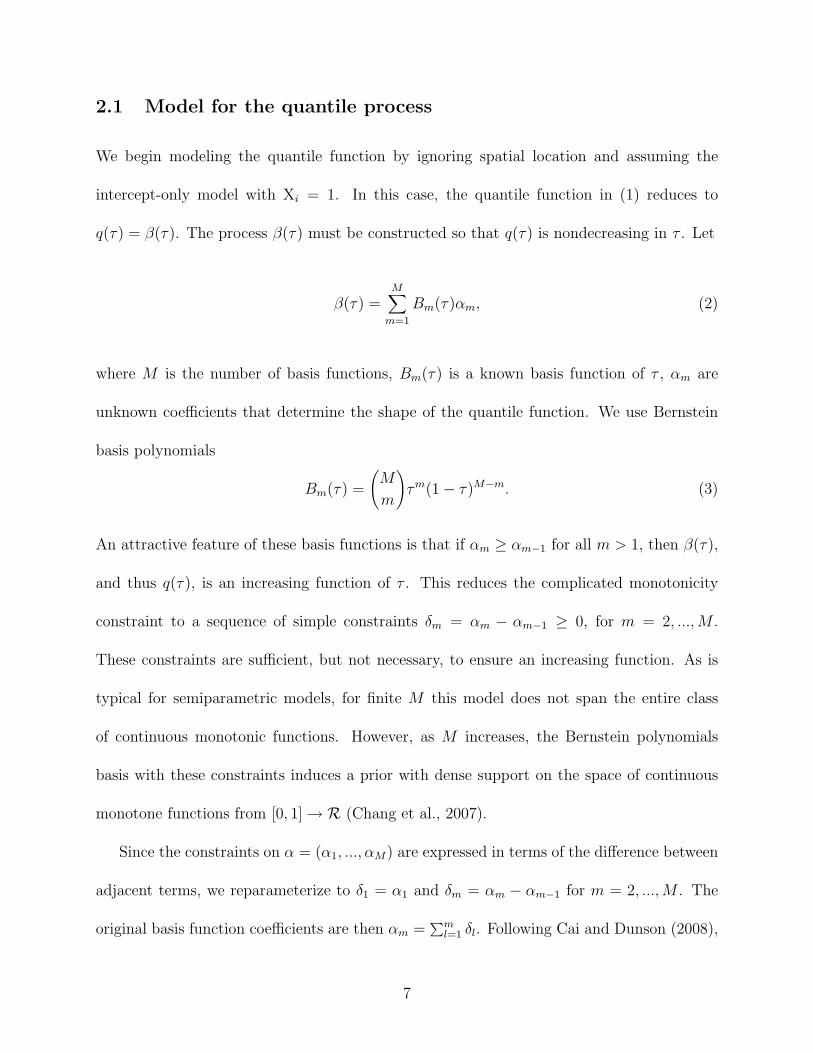
2.1 Model for the quantile process

We begin modeling the quantile function by ignoring spatial location and assuming the

intercept-only model with Xi = 1. In this case, the quantile function in (1) reduces to

q(τ) = β(τ). The process β(τ) must be constructed so that q(τ) is nondecreasing in τ . Let

β(τ) =M∑

m=1

Bm(τ)αm, (2)

where M is the number of basis functions, Bm(τ) is a known basis function of τ , αm are

unknown coefficients that determine the shape of the quantile function. We use Bernstein

basis polynomials

Bm(τ) =

(M

m

)τm(1− τ)M−m. (3)

An attractive feature of these basis functions is that if αm ≥ αm−1 for all m > 1, then β(τ),

and thus q(τ), is an increasing function of τ . This reduces the complicated monotonicity

constraint to a sequence of simple constraints δm = αm − αm−1 ≥ 0, for m = 2, ..., M .

These constraints are sufficient, but not necessary, to ensure an increasing function. As is

typical for semiparametric models, for finite M this model does not span the entire class

of continuous monotonic functions. However, as M increases, the Bernstein polynomials

basis with these constraints induces a prior with dense support on the space of continuous

monotone functions from [0, 1] → R (Chang et al., 2007).

Since the constraints on α = (α1, ..., αM) are expressed in terms of the difference between

adjacent terms, we reparameterize to δ1 = α1 and δm = αm − αm−1 for m = 2, ..., M . The

original basis function coefficients are then αm =∑m

l=1 δl. Following Cai and Dunson (2008),

7

we ensure the quantile constraint by introducing a latent unconstrained variable δ∗m and

taking δ1 = δ∗1 and

δm =

δ∗m, δ∗m ≥ 0

0, δ∗m < 0

(4)

for m > 1.

The δ∗m have independent normal priors δ∗m ∼ N(δm(Θ), σ2), with unknown hyperparam-

eters Θ. We pick δm(Θ) to center the quantile process on a parametric distribution f0(y|Θ),

for example, a N(µ0, σ20) random variable with Θ = (µ0, σ0). Letting q0(τ |Θ) be the quantile

function of f0(y|Θ), the δm(Θ) are then chosen so that

q0(τ |Θ) ≈M∑

m=1

Bm(τ)αm(Θ), (5)

where αm(Θ) =∑m

l=1 δl(Θ). The δm(Θ) are chosen to correspond to the following ridge

regression estimator:

(δ1(Θ), ..., δM(Θ)

)′= arg min

d

K∑

k=1

(q0(τk|Θ)−

M∑

m=1

Bm(τk)

[m∑

l=1

dl

])2

+ λM∑

m=1

d2m, (6)

where dm ≥ 0 for m > 1, τ1, ..., τK is a dense grid on (0,1). We find that simple paramet-

ric quantile curves can often be approximated almost perfectly with fewer than M terms.

Therefore several combinations of d give essentially the same fit, including some undesir-

able solutions with negative values for elements of δ. For numerical stability we add the

ridge penalty λ∑M

m=1 d2m. Setting the tuning constant λ to zero gives the unpenalized fit

and setting λ to infinity gives δ = 0 for all terms. We pick λ = 1 because this allows the

8

parametric quantile curve to be approximated well and gives δ values that vary smoothly

from term-to-term. As σ → 0, the quantile functions this resembles are increasing shrunk

towards the parametric quantile function q0(τ |Θ), and the likelihood is similar to f0(y|Θ).

2.2 Model for the spatial quantile process with covariates

Adding covariates, the conditional quantile function becomes

q(τ |Xi) = X′iβ(τ) =

p∑

j=1

Xijβj(τ). (7)

As in Section 2.1, the quantile curves are modeled using Bernstein basis polynomials

βj(τ) =M∑

m=1

Bm(τ)αjm, (8)

where αjm are unknown coefficients. The processes βj(τ) must be constructed so that q(τ |Xi)

is nondecreasing in τ for all Xi. Collecting terms with common basis functions gives

X′iβ(τ) =

M∑

m=1

Bm(τ)θm(Xi), (9)

where θm(Xi) =∑p

j=1 Xijαjm. Therefore, if θm(Xi) ≥ θm−1(Xi) for all m > 1, then X′iβ(τ),

and thus q(τ |Xi), is an increasing function of τ .

To specify our prior for the αjm to ensure monotonicity, we assume that Xi1 = 1 for

the intercept and the remaining covariates are suitably scaled so that Xij ∈ [0, 1] for j > 1.

Since the constraints are written in terms of the difference between adjacent terms, we

9

reparameterize to δj1 = αj1 and δjm = αjm−αjm−1 for m = 2, ...,M . We ensure the quantile

constraint by introducing latent unconstrained variable δ∗jm ∼ N(δjm(Θ), σ2j ) and taking

δjm =

δ∗jm, δ∗1m +∑p

j=2 I(δ∗jm < 0)δ∗jm ≥ 0

0, otherwise

(10)

for all j = 1, ..., p and m = 1, ..., M . Recalling Xi1 = 1 and Xij ∈ [0, 1] for j = 2, ..., p, and

thus Xijδjm ≥ XijI (δjm < 0) δjm ≥ I (δjm < 0) δjm for j > 1,

θm(Xi)− θm−1(Xi) =p∑

j=1

Xijδjm ≥ δ1m +p∑

j=2

XijI (δjm < 0) δjm (11)

≥ δ1m +p∑

j=2

I (δjm < 0) δjm ≥ 0

for all Xi, giving a valid quantile process. As in Section 2.1 we center the intercept curve on

a parametric quantile function q0(Θ). The remaining coefficients have δjm(Θ) = 0 for j > 1.

Although this model is quite flexible, we have assumed that the quantile process is a

linear function of the covariates, simplifying interpretation. In some applications the linear

quantile relationship may be overly-restrictive. In this case, transformations of the original

predictors such as interactions or basis functions can be added to give a more flexible model.

However, (10) may be prohibitive if quadratic or higher-order terms are added to the model

since (10) unnecessarily restricts the quantile function for combinations of the covariates

that can never occur, for example, the linear term being zero and the quadratic term being

one. Also, the linear relationship between the predictors and the response is not invariant to

transformations of the response. To alleviate some sensitivity to transformations, it may be

10

possible to develop a nonlinear model for q(τ |Xi), so that q(τ |Xi) and T (q(τ |Xi)) span the

same class of functions (and therefore response distributions) for a class of transformations

T .

For spatial data, we allow the quantile process to be different at each spatial location,

βj(τ, s) =M∑

m=1

Bm(τ)αjm(s), (12)

where αjm(s) are spatially-varying basis function coefficients. We enforce the monotonicity

constraint at each spatial location by introducing latent Gaussian parameters δ∗jm(s). The

latent parameters relate to the basis function coefficients as αjm(s) =∑m

l=1 δjl(s) and

δjm(s) =

δ∗jm(s), δ∗1m(s) +∑p

j=2 I(δ∗jm(s) < 0)δ∗jm(s) ≥ 0

0, otherwise

(13)

for all j = 1, ..., p and m = 1, ..., M .

To encourage the conditional density functions to vary smooth across space we model the

δ∗jm(s) as spatial processes. The δ∗jm(s) are independent (over j and m) Gaussian spatial pro-

cesses with mean E(δ∗jm(s)) = δjm(Θ) and exponential spatial covariance Cov(δ∗jm(s), δ∗jm(s′)) =

σ2j exp (−||s− s′||/ρj), where σ2

j is the variance of δ∗jm(s) and ρj determines the range of the

spatial correlation function.

11

3 Approximate method

Section 2’s spatial quantile regression model can be implemented efficiently for moderately-

sized data sets. However, it becomes computationally infeasible for Section 5.3’s analysis of

several years of daily data for the Eastern U.S. To approximate the full Bayesian analysis, we

propose a two-stage approach related to that of Daniels and Kass (1999). We first perform

separate quantile regression at each site for a grid of quantile levels to obtain estimates of

the quantile process and their asymptotic covariance. In a second stage, we analyze these

initial estimates using the Bayesian spatial model for the quantile process.

The usual quantile regression estimate (Koenker, 2005) for quantile level τk and spatial

location s is

(β1(τk, s), ..., βp(τk, s)

)′= arg min

β

∑

si=s, yi>X′iβ

τk|yi−X′iβ|+

∑

si=s, yi<X′iβ

(τk−1)|yi−X′iβ|. (14)

This estimate is easily obtained from the quantreg package in R and is consistent for the true

quantile function and has asymptotic covariance (Koenker, 2005)

Cov[√

ns(β1(τk, s), ..., βp(τk, s)

),√

ns

(β1(τl, s), ..., βp(τl, s)

)]= H(τk)

−1J(τk, τl)H(τl)−1,

(15)

where ns is the number of observations at site s, H(τ) = limns→∞ n−1s

∑nsi=1 XiX

′ifi(X

′iβ(τ)),

fi(X′iβ(τ)) is the conditional density of yi evaluated at X′

iβ(τ), and J(τk, τl) = [τk ∧ τl − τkτl] n−1s

∑XiX

′i.

Although consistent as the number of observations at a given site goes to ∞, these esti-

mates are not smooth over space or quantile level, and do not ensure a non-crossing quantile

function for all X. Therefore we smooth these initial estimates using the spatial model for the

12

quantile process proposed in Section 2. Let β(si) =[β1(τ1, si), ..., β1(τK , si), β2(τ1, si), ..., βp(τK , si)

]′

and cov(β(si)

)= Σi (with elements defined by (15)). We fit the model

β(si) ∼ N (β(si),Σi) , (16)

where the elements of β(si) = [β1(τ1, si), ..., β1(τK , si), β2(τ1, si), ..., βp(τK , si)]′ are functions

of Bernstein basis polynomials as in Section 2.2. This approximation provides a dramatic

reduction in computational time because the dimension of the response is reduced from the

number of observations at each site to the number of quantile levels in the approximation,

and the posteriors for the parameters that define β are fully-conjugate allowing for Gibbs

updates and rapid convergence.

The correlation between initial estimates is often very high. To avoid numerical instability

we pick the number of quantile levels in the initial estimate, K, so that the estimated

correlation is no more than 0.95. For the simulated and real data, we use K = 10. Also, our

experience with this approximation suggests that this approximation has coverage probability

below the nominal level. Therefore, we inflate the estimated variance by a factor of c2

and fit the model β(si) ∼ N (β(si), c2Σi). We pick c by first fitting the model with c =

1. We then generate R data sets from the fitted model, analyze each data set with c =

0.5, 0.75, 1, 1.25, 1.5, and compute the proportion (averaged over space, quantile level, and

covariate) of the 90% intervals that cover the coefficients used to generate the data. We

pick the smallest c with 90% coverage. For large data sets with many locations and several

covariates we find R = 1 is sufficient to give reasonable coverage probabilities.

This simplification may permit extensions to more sophisticated spatial models for the

13

basis coefficients, such as non-stationary and non-Gaussian spatial models. Details of the

MCMC algorithm for this model and the full model are given in the Appendix. It may also

be possible to develop an EM-type algorithm or a constrained optimization routine, although

MCMC is well-suited as described above.

4 Simulation study

In this section we analyze simulated data to compare our method with standard quantile

regression approaches, and to examine the performance of Section 3’s approximate method.

For each of the S = 50 simulated data sets we generate n = 20 spatial locations si uniformly

on [0, 1]2. The p = 3 covariates are generated as X1 ≡ 1 and Xi2, Xi3iid∼ U(0,1), independent

over space and time. The true quantile function is

q(τ |Xi, si) = 2si2 + (τ + 1)Φ−1(τ) +(5si1τ

2)Xi3, (17)

which implies that β1(τ, si) = 2si2+(τ +1)Φ−1(τ), β2(τ, si) = 0, and β3(τ, si) = 5si1τ2, where

Φ is the standard normal distribution function. Figure 1a plots the density corresponding to

this quantile function for various covariates and spatial locations. The density is generally

right-skewed to mimic ozone data. The second spatial coordinate simply shifts the entire

distribution by increasing the intercept function β1. The first predictor X2 has no effect on

the density because β2(τ, s) = 0. The second predictor X3 has little effect on the left tail

because β3(τ, s) is near zero for small τ , but increasing X3 adds more mass to the density’s

right tail.

14

Figure 1: True and estimated quantile curves for the simulation study. Panel (a) gives thetrue density as a function of space and covariates. Panel (b) plots the true quantile functionβ3(s, τ), Panel (c) plots the usual quantile estimate for one data set, and Panel (d) plots theposterior mean from spatial quantile regression for one data set.

−2 0 2 4 6 8 10

0.00

00.

001

0.00

20.

003

0.00

4

y

dens

ity

s=(0.0,0.0), x3=0.0s=(0.0,1.0), x3=0.0s=(0.5,0.0), x3=0.5s=(1.0,0.0), x3=1.0

0.2 0.4 0.6 0.8

−2

−1

01

23

45

τ

β 3(τ

, s)

(a) True density (b) True β3 by location

0.2 0.4 0.6 0.8

−2

−1

01

23

45

τ

β 3(τ

, s)

0.2 0.4 0.6 0.8

−2

−1

01

23

45

τ

β 3(τ

, s)

(c) Usual quantile regression estimate (d) Bayesian spatial quantile regression estimate

15

Each data set contains 100 replicates at each spatial location. We first consider the situ-

ation where the replicates are independent over space and time. We also generate data with

spatially and temporally correlated residuals using a Gaussian copula. To generate spatially-

correlated residuals, we first generate Ui as independent (over time) Gaussian processes with

mean zero and exponential spatial covariance exp (−||s− s′||/ρZ), and then transform using

the marginal quantile function yi = qo[Φ(Ui)] +∑M

m=1 Bm[Φ(Ui)]θm(Xi, si). We assume the

spatial range of the residuals is ρZ = 0.5. We also generate data with no spatial correlation,

but temporal correlation at each site. The latent Gaussian process at each site has mean

zero and exponential covariance Cor(Ui, Uj) = exp (−|i− j′|/ρU), where ρU = −1/ log(0.5)

so the correlation between subsequent sites is 0.5.

For each simulated data set we fit three Bayesian quantile methods: the full model de-

scribed in Section 2, the model in Section 2 without spatial modeling (i.e., δ∗jkiid∼ N(δjk(Θ), σ2

j )),

and Section 3’s approximate method. For the Bayesian quantile regression models (full and

approximate) we use M = 10 knots and vague yet proper priors for the hyperparameters

that control the prior covariance of the quantile function, σ2j ∼ InvG(0.1,0.1) and ρj ∼

Gamma(0.06,0.75). The prior for the ρj is selected so the effective range −ρj log(0.05), i.e.,

the distance at which the spatial correlation equals 0.05, has prior mean 0.25 and prior stan-

dard deviation 1. The centering distribution f0 was taken to be skew-normal (Azzalini, 1985)

with location µ0 ∼ N(0,102), scale σ20 ∼ InvGamma(0.1,0.1), and skewness ψ0 ∼ N(0,102).

We also compare our methods with the usual frequentist estimates in (14), computed using

the quantreg package in R. Of course these estimates do not smooth over quantile level or

spatial location, so they may not be directly comparable in this highly-structured setting.

For each simulated data set and each method we compute point estimates (posterior

16

means for Bayesian methods) and 90% intervals for βj(τk, si) for j = 1, 2, 3, τk ∈ 0.05, 0.10, ..., 0.95,

and all spatial locations si. We compare methods using mean squared error, coverage prob-

ability, and power (i.e., the proportion of times in repeated samples under the alternative

that the 90% interval excludes zero) averaged over space, quantile levels, and simulated data

set. Specifically, mean squared error for the jth quantile function is computed as

MSE =1

SnK

S∑

sim=1

n∑

i=1

K∑

k=1

(βj(τk, si)

(sim) − βj(τk, si))2

, (18)

where βj(τk, si)(sim) is the point estimate for the simulation number sim. Coverage and

power are computed similarly.

Table 1 presents the results. We first discuss the results without residual correlation.

By borrowing strength across quantile level and spatial location all three Bayesian methods

provide smaller mean squared error and higher power than the usual quantile regression

approach. Figure 1b shows the true quantile curve for β3 for each spatial location for one

representative data set with line width proportional to the first spatial coordinate. The usual

estimates in Figure 1c fluctuate greatly across quantile levels compared to the smooth curves

produced by the Bayesian spatial quantile regression model in Figure 1d.

The approximate method which smooths the initial estimates from usual quantile re-

gression reduces mean squared error. In fact, in this simulation the approximate method

often has smaller mean squared error than the full model. Therefore, the approximate model

appears to provide a computationally efficient means to estimate the true quantile function

to be used for predicting future observations. However, the full model gives higher power

for the non-null coefficient β3.

17

Table 1: Simulation study results. MSE and coverage probabilities are averaged over spatiallocation, simulated data set, and quantile level. Power is evaluated only for the 95th quantilelevel for β3 and is averaged over space and simulated data set.

Corr. MSE Coverage PowerMethod Resids β1 β2 β3 β1 β2 β3 β3

Quantreg None 0.51 (0.06) 0.99 (0.11) 1.02 (0.11) 0.89 0.89 0.88 0.35Bayes - Approx 0.09 (0.01) 0.13 (0.01) 0.23 (0.03) 0.87 0.91 0.88 0.44Bayes - Full nonspatial 0.31 (0.04) 0.21 (0.02) 0.62 (0.08) 0.82 0.93 0.85 0.57Bayes - Full spatial 0.13 (0.02) 0.12 (0.01) 0.27 (0.04) 0.86 0.93 0.88 0.79Quantreg Space 0.53 (0.06) 1.02 (0.11) 1.03 (0.11) 0.89 0.88 0.88 0.36Bayes - Approx 0.10 (0.01) 0.11 (0.01) 0.21 (0.03) 0.83 0.92 0.88 0.45Bayes - Full nonspatial 0.32 (0.05) 0.20 (0.01) 0.65 (0.08) 0.82 0.92 0.84 0.58Bayes - Full spatial 0.14 (0.02) 0.10 (0.01) 0.23 (0.03) 0.84 0.93 0.88 0.81Quantreg Time 0.56 (0.06) 0.94 (0.10) 1.03 (0.11) 0.89 0.88 0.88 0.36Bayes - Approx 0.13 (0.01) 0.11 (0.01) 0.27 (0.03) 0.85 0.91 0.88 0.49Bayes - Full nonspatial 0.33 (0.04) 0.16 (0.01) 0.63 (0.08) 0.79 0.93 0.84 0.30Bayes - Full spatial 0.15 (0.02) 0.10 (0.01) 0.23 (0.03) 0.72 0.86 0.79 0.59

Adding residual correlation does not affect mean square error. Spatial correlation in

the residuals has a small effect on the coverage probabilities, perhaps because the spatially-

varying regression parameters absorb some of the residual correlation. However, adding

temporal correlation reduces the coverage probability below 0.8. Therefore, strong residual

correlation should be accounted for, perhaps using a copula model as discussed in Section 6.

In this simulation we assumed M = 10 basis functions, σ2j ∼ InvGamma(0.1,0.1), and

the prior standard deviation of the effective range was one. We reran the simulation (with

independent residuals) with S = 10 data sets using the full model three times, each vary-

ing one of these assumptions. The alternatives were M = 25 basis functions, σj ∼ In-

vGamma(0.001,0.001), and the prior standard deviation of the effective range set to five.

The results of the simulation were fairly robust to these changes; the mean squared error

varied from 0.06 to 0.11 for X1, from 0.07 to 0.12 for X2, and from 0.18 to 0.26 for X3,

18

and the average coverage probability was at least 0.86 for all fully Bayes models and all

covariates. The prior for the effective range was most influential. Altering this prior affected

the posterior of the spatial range, but had only a small effect on the mean squared errors

and coverage probabilities.

5 Analysis of Eastern US ozone data

In this section we analyze monitored ozone data from the Eastern US from the summers

of 1997-2005 and climate model output from 2041-2045. Section 5.1 describes the data.

Sections 5.2 and 5.3 analyze monitored ozone data from 1997-2005, first using the full model

and a subset of the data, and then using Section 3’s approximate model and the complete

data. Sections 5.4 and 5.5 analyze the computer model output.

5.1 Description of the data

Meteorological data were obtained from the National Climate Data Center (NCDC;

http://www.ncdc.noaa.gov/oa/ncdc.html). We obtained daily average temperature and

daily maximum wind speed for 773 monitors in the Eastern US from the NCDC’s Global

Summary of the Day Data Base. Daily average cloud cover for 735 locations in the Eastern

US was obtained from the NCDC’s National Solar Radiation Data Base.

Maximum daily 8-hour average ozone was obtained from the US EPA’s Air Explorer Data

Base (http://www.epa.gov/airexplorer/index.htm). We analyze daily ozone concentrations

measured at 631 locations in the Eastern US during the summers (June-August) of 1997-

2005 (470,239 total observations), plotted in Figure 2a. Meteorological and ozone data are

19

not observed at the same locations. Therefore we imputed meteorological variables at the

ozone locations using spatial Kriging. Spatial imputation was performed using SAS version

9.1 and the MIXED procedure with spatial exponential covariance function, with covariance

parameters allowed to vary by variable and year. We treat these predictors as fixed. Li,

Tang, and Lin (2009) discuss the implications of ignoring uncertainty in spatial predictors.

Temperature and cloud cover are fairly smooth across space and thus have small interpolation

errors, however there is more uncertainty in the wind speed interpolation. Accounting for

uncertainty in the predictors using a spatial model for the meteorological variables warrants

further consideration.

The final source of data is time slice experiments from the North American Regional

Climate Change Assessment Program (http://www.narccap.ucar.edu/data/). These data

are output from the Geophysical Fluid Dynamics Laboratory’s (GFDL) deterministic at-

mospheric computer model (AM2.1) with 3 hour × 50 km resolution. We use data from

two experiments. The first provides modeled data from 1968 to 2000 using observed sea

surface temperature and sea-ice extent. These data are a reanalysis using boundary con-

ditions determined by actual historical data. The second provides modeled data for 2038

to 2070 using deviations in sea surface temperature and sea-ice extent from the GFDL’s

CM2.1 A2 scenario. From these experiments we obtain modeled daily average temperature,

maximum wind speed, and average cloud cover fraction. These gridded data do not have the

same spatial support as ozone and meteorology data obtained from point-reference monitors.

Throughout we use the ozone monitoring locations as the spatial unit, and we match mod-

eled climate data with ozone data by extracting climate data from the grid cell containing

the ozone monitor.

20

Figure 2: Panel (a) maps the sample median ozone concentration; the points are the 631monitoring locations. Panel (b) plots the skew-normal(34.5,24.3,1.8) over the histogram ofozone concentrations, pooled over spatial location. Panels (c) and (d) plot ozone by dailyaverage temperature and cloud cover proportion, respectively; the data are pooled over spaceand the width of the boxplots are proportional to the number of observations in the bins.

−90 −85 −80 −75 −70

3035

4045

30

40

50

60

Fre

quen

cy

0 20 40 60 80 100 120

050

0010

000

1500

020

000

2500

0

(a) Median ozone (ppb) (b) Histogram of ozone (ppb)

6 10 14 18 22 26 30 34

020

4060

8010

0

0 15 30 45 60 75 90

020

4060

8010

0

(c) Ozone by temperature (C) (d) Ozone by cloud cover (%)

21

5.2 Atlanta sub-study

We begin by comparing several models using only data from the 12 stations in the Atlanta

area. The continuous variables temperature and wind speed are standardized and trans-

formed to the unit interval (as assumed in the monotonicity constraints described in Section

2) by the normal CDF

Xj = Φ ([temp−m(temp)]/s(temp)) (19)

where m(temp) and s(temp) are the sample mean and standard deviation of daily tempera-

ture over space and time. Cloud cover proportion naturally falls on the unit interval. We also

include the year to investigate temporal trends in the quantile process. The year is trans-

formed as Xj = (year−1997)/8. We also include the interaction XjXl between temperature

and cloud cover and quadratic effects 4(Xj − 0.5)2.

We fit the full and approximate model with and without quadratic terms and compare

these models with the fully-Gaussian spatial model with spatially-varying coefficients,

y(s, t) =p∑

j=1

Xj(s, t)βj(s) + µ(s, t) + ε(s, t), (20)

where βj(s) are spatial Gaussian processes with exponential covariance, µ(s, t) are inde-

pendent (over time) spatial Gaussian processes with exponential covariance, and ε(s, t)iid∼

N(0, σ2) is the nugget effect. For both the full and approximate Bayesian quantile regres-

sion models, the centering distribution f0 is taken to be skew-normal with location µ0 ∼

N(0,102), scale σ20 ∼ InvGamma(0.1,0.1), and skewness ψ0 ∼ N(0,102). Figure 2b shows

that this distribution is flexible enough to approximate the ozone distributions. However,

22

the parametric mean regression model with parametric skew-normal errors would not allow

for the shape of the right tail to depend on covariates. We note that the quantile regression

models do not explicitly model spatial or temporal association in the daily ozone values.

Effects of residual correlation are examined briefly in Section 5.5 and alternative models are

discussed in Section 6. We use M = 10 knots and priors τ 2jm ∼ InvGamma(0.1,0.1) and

ρj ∼ Gamma(0.5,0.5), which gives prior 95% intervals (0.00,0.99) and (0.00,0.80) for the

correlation between the closest and farthest pairs of points, respectively.

To compare models we randomly removed all observations for 10% of the days (N =

910 total observations), with these test observations labeled y∗1, ..., y∗N . For each deleted

observation we compute the posterior predictive mean y∗i and the posterior predictive 95%

equal-tailed intervals. Table 2 gives the root mean squared prediction error RMSE =

√∑Ni=1 (y∗i − y∗i )

2 /N , mean absolute deviation MAD =∑N

i=1 |y∗i − y∗i |/N , and the coverage

probabilities and average (over i) width of the prediction intervals. Note that the RMSEs

reported here are larger than those reported by other spatial analyses of ozone data, e.g.

Sahu et al. (2007), that withhold all observations for some sites, rather than all observations

for some days. In contrast, we withhold all observations on a subset of days, and therefore

our predictions rely entirely on correctly modeling the relationship between meteorology and

ozone, and do not use spatial interpolation. Since ozone shows a strong spatial pattern, this

results in higher RMSE. We feel this approach to cross-validation is more relevant for our

goal of prediction for future days without any observed values.

The coverage probabilities of the 95% intervals are near or above the nominal rate for

all models in Table 2. The Gaussian models have the highest RMSE and MAD. To test

for a possible transformation to normality, we also fitted the Gaussian model using the

23

Table 2: Cross-validation results for the Atlanta sub-study.

Coverage Prob Average WidthModel Covariates 95% interval 95% interval RMSE MADGaussian Linear 0.965 60.4 14.3 9.34Gaussian Quadratic 0.969 59.8 14.2 9.07QR - approx Linear 0.959 50.4 13.1 7.76QR - approx Quadratic 0.947 47.3 12.9 7.62QR - full Linear 0.987 70.1 13.2 7.87QR - full Quadratic 0.986 69.6 13.0 7.64

square root of ozone as the response. RMSE and MAD are compared by squaring the

draws from the predictive distribution. RMSE (14.4 for linear predictors, 14.2 for quadratic

predictors) and MAD (9.6 for linear predictors, 9.2 for quadratic predictors) were similar to

the untransformed response, so we use the untransformed response for ease of interpretation.

The approximate method with quadratic terms minimizes both RMSE and MAD, has good

coverage probability, justifying its use for prediction.

Figure 3 summarizes the posterior for the full Bayesian spatial quantile regression model

with quadratic terms. Panels (a)-(c) plot the quantile curves for one representative location.

The main effects are all highly significant, especially for the upper quantile levels. As ex-

pected ozone concentration increases with temperature and decreases with cloud cover and

wind speed. Figure 3 reveals a complicated relationship between ozone and temperature.

The linear temperature effect is near zero for low quantile levels and increases with τ .

Figure 3c plots the data and several fitted quantile curves (τ ranging from 0.05 to 0.95) by

year with the transformed meteorological variables fixed at 0.5. All quantile levels decrease

from 1997 to 2002; after 2002 the lower quantiles plateau while the upper quantiles continue

to decline. Note that in this plot more than 5% of the observations fall above the 95% quantile

24

Figure 3: Results for Atlanta sub-study. Panels (a)-(c) plot the results for one location.Panels (a) and (b) give posterior 95% intervals for main effect and second-order quantilecurves. Panel (c) plots the data by year, along with the posterior mean quantile curves forseveral quantile levels ranging from τ = 0.05 to τ = 0.95 with all covariates fixed at 0.5expect year. Panel (d) plots the posterior mean of the year main effect for each location.

0.0 0.2 0.4 0.6 0.8 1.0

−40

−20

020

τ

β(τ)

TemperatureCloud CoverWind SpeedYearTemp*Cloud Cover

0.0 0.2 0.4 0.6 0.8 1.0

−10

−5

05

1015

τ

β(τ)

TemperatureCloud CoverWind speedYear

(a) Linear terms (b) Quadratic terms

1998 2000 2002 2004

2040

6080

100

120

Year

q(τ)

0.0 0.2 0.4 0.6 0.8 1.0

−40

−30

−20

−10

0

τ

β(τ)

(c) Data and fit by year (d) Year main effect by location

25

level. This is the result of plotting the quantile functions without regard to variability in the

meterological variables (i.e., fixing them at 0.5). To give a sense of the spatial variability

in the quantile curves, Figure 3d plots the posterior mean of the main effect for year for

all locations. All sites show a decreasing trend, especially for upper quantile levels. The

decreasing trends are adjusted for meteorology, and may be explained by other factors, such

as emission reductions. There is considerable variation from site-to-site. The posterior 95%

interval for the difference between the year main effect at τ = 0.8 for the sites with largest

and smallest posterior mean is (10.4, 25.0).

5.3 Analysis of Eastern US ozone data

Analyzing data for the entire Eastern US using the full Bayesian spatial quantile regression

model is not computationally feasible, so we use only the approximate model. We selected

variance inflation c = 1. We considered other values of c, but the estimates were nearly

identical so we pick c=1 for simplicity. Based on Section 5.2’s results, we include quadratic

terms for all predictors. Also, we use the same priors as in Section 5.2. The posterior

median (95% interval) for the skewness parameter ψ0 of the skew-normal base distribution is

3.76 (1.12, 10.54), supporting a non-Gaussian analysis. To justify that this model fits well,

we randomly removed observations for 2% of the days (N = 12, 468 observations) and the

out-of-sample coverage probability of the 95% prediction intervals was 93.4%.

Figure 4 maps the posterior means of several quantile functions. The two strongest

predictors are temperature and cloud cover. The model includes interaction and quadratic

terms, so to illustrate the effects, we plot linear combinations of all terms involving these

26

predictors,

X1β1(τ, s) + X2β2(τ, s) + 4(X1 − 0.5)2β3(τ, s) + 4(X2 − 0.5)2β4(τ, s) + X1X2β5(τ, s), (21)

where X1 and X2 are temperature and cloud cover values, respectively, and β1-β5 are the

corresponding quantile curves. Figure 4a-4d plot the posterior means of linear combinations

using X1 that correspond to 20oC and 30oC and X2 that correspond to 10% and 90% cloud

cover.

For both temperature values ozone concentrations are generally higher when cloud cover

is low. For clear days with 10% cloud cover temperature has a strong effect on ozone in

the north, but only a weak effect in the south. For cloudy days with 90% cloud cover,

temperature has less effect overall, but remains significant in the northeast.

The linear time trend for the 95th quantile in Figure 4e is generally decreasing, especially

in the south. This agrees with Chan (2009). To compare the rate of decrease in the upper

and lower tails, Figure 4f plots the difference between the linear time trend for the 95th

and 5th quantile (βj(0.95, s) − βj(0.05, s)). In the Mid-Atlantic (red) the negative trend is

stronger in the lower tail than the upper tail; in contrast in Florida the trend is stronger in

the upper tail.

5.4 Calibrating computer model output

Before applying our statistical model to project ozone levels, we must calibrate the climate

model with the observed data. For example, calibration is necessary to account for systematic

differences between grid cell averages and point measurements. Figure 5 plots the sample

27

Figure 4: Summary of the posterior mean of βj(τ, s). Panels (a)-(d) plot linear combinationsof βj(τ, s) as discussed in (21). Panels (e) and (f) plot the posterior mean of βj(0.95, s) andβj(0.95, s)− βj(0.05, s), respectively. The units are parts per billion in all plots.

−90 −85 −80 −75 −70

3035

4045

−40

−20

0

20

40

−90 −85 −80 −75 −70

3035

4045

−40

−20

0

20

40

(a) 20o C, cloud cover 10%, τ = 0.95 (b) 30o C, cloud cover 10%, τ = 0.95

−90 −85 −80 −75 −70

3035

4045

−40

−20

0

20

40

−90 −85 −80 −75 −70

3035

4045

−40

−20

0

20

40

(c) 20o C, cloud cover 90%, τ = 0.95 (d) 30o C, cloud cover 90%, τ = 0.95

−90 −85 −80 −75 −70

3035

4045

−60

−40

−20

0

20

−90 −85 −80 −75 −70

3035

4045

−20

−15

−10

−5

0

5

(e) Linear year, τ = 0.95 (f) Linear year, τ = 0.95 - τ = 0.0528

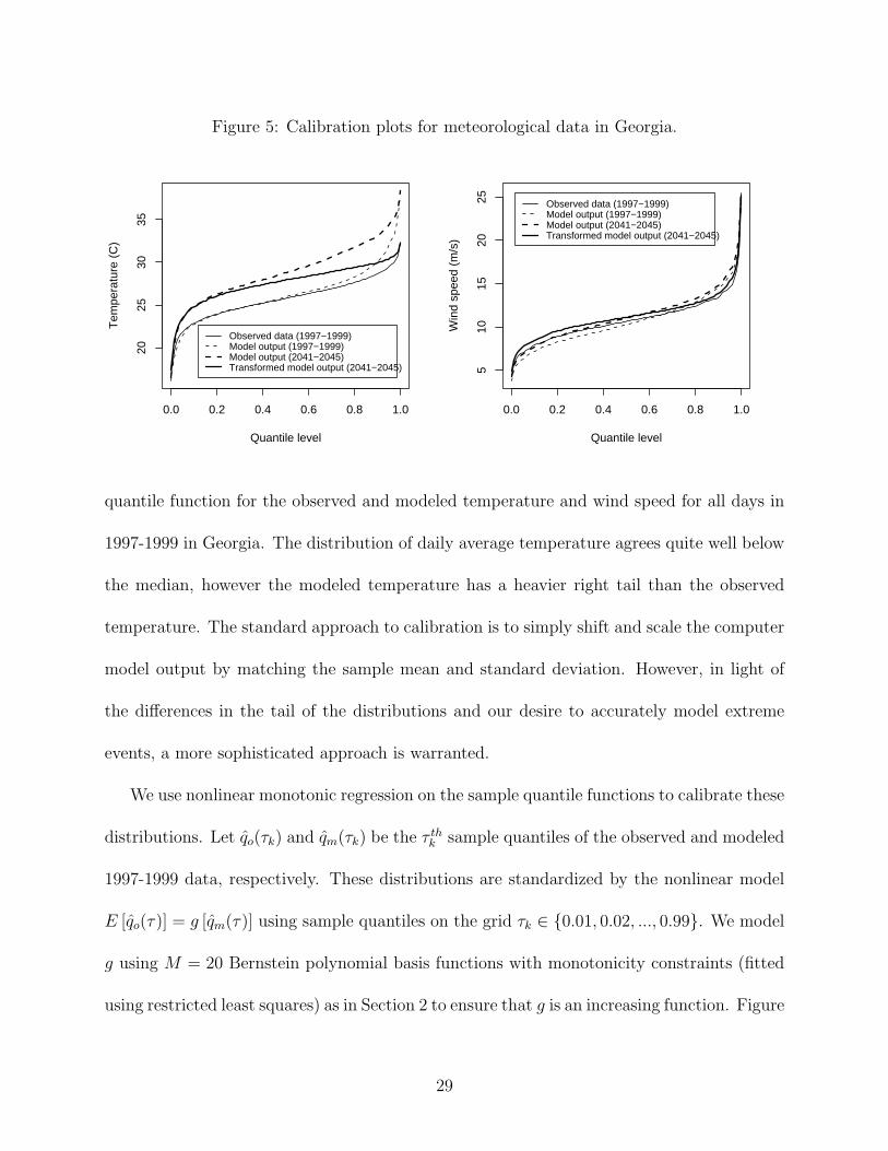
Figure 5: Calibration plots for meteorological data in Georgia.

0.0 0.2 0.4 0.6 0.8 1.0

2025

3035

Quantile level

Tem

pera

ture

(C

)

Observed data (1997−1999)Model output (1997−1999)Model output (2041−2045)Transformed model output (2041−2045)

0.0 0.2 0.4 0.6 0.8 1.0

510

1520

25

Quantile levelW

ind

spee

d (m

/s)

Observed data (1997−1999)Model output (1997−1999)Model output (2041−2045)Transformed model output (2041−2045)

quantile function for the observed and modeled temperature and wind speed for all days in

1997-1999 in Georgia. The distribution of daily average temperature agrees quite well below

the median, however the modeled temperature has a heavier right tail than the observed

temperature. The standard approach to calibration is to simply shift and scale the computer

model output by matching the sample mean and standard deviation. However, in light of

the differences in the tail of the distributions and our desire to accurately model extreme

events, a more sophisticated approach is warranted.

We use nonlinear monotonic regression on the sample quantile functions to calibrate these

distributions. Let qo(τk) and qm(τk) be the τ thk sample quantiles of the observed and modeled

1997-1999 data, respectively. These distributions are standardized by the nonlinear model

E [qo(τ)] = g [qm(τ)] using sample quantiles on the grid τk ∈ 0.01, 0.02, ..., 0.99. We model

g using M = 20 Bernstein polynomial basis functions with monotonicity constraints (fitted

using restricted least squares) as in Section 2 to ensure that g is an increasing function. Figure

29

5 shows the transformed temperature for Georgia. Model outputs for 2041-2045 with large

temperatures are reduced to resolve the discrepancy between observed and modeled 1997-

1999 data. The meteorological predictors are transformed separately by state to account for

spatial variation in the calibration.

We compare this calibration method to the simple method of adjusting each site by the

state mean and variance using five-fold cross-validation. We randomly divided the observed

temperature data into 5 groups. For each group we used the observations from the remain-

ing four groups to calibrate the computer model output for the group. For each site, we

computed the squared difference between the mean observed temperature and the mean of

the calibrated computer output, as well as the Kolmogorov-Smirnov test statistic for the

test that the observed temperature and calibrated computer model output follow the same

distribution. The quantile calibration method has smaller squared error (average of 3.26

compared to 3.31, smaller at 56% of sites) and KS-statistic (average of 0.139 compared to

0.149, smaller at 59% of sites) than the mean/variance calibration method.

5.5 Projecting ozone levels under different climate scenarios

The additive structure of the quantile regression model gives the effect of each covariate on

the maximum daily 8-hour average ozone in closed form. In addition, policy makers are

often interested in the effect of covariates on the yearly ozone distribution. For example, in

this section we explore the relationship between temperature and yearly median and 95th

percentile of ozone. Here we use Section 5.3’s estimate of the conditional density of daily

ozone to simulate several realizations of the ozone process to forecast yearly summaries under

30

different climate scenarios. These simulations vary temperature, wind speed, and cloud cover

and assume all other factors (emissions, land-use, etc.) are fixed. Certainly other factors

will change in the future (for example emissions may decline in response to new standards)

so these projections are not meant to be realistic predictions. Rather, they are meant to

isolate the effect of climate change on future ozone levels.

Two factors contribute to the effect of climate changes on ozone levels at a given location:

the magnitude of the climate change and the strength of the association of meteorology and

ozone. To quantify spatial variability in the effect of temperature increase on yearly sum-

maries, we generate 500 replicates of the ozone process at the data points under different

climate scenarios. The first scenario is no change in the meteorological variables. In this

case, replicates are generated by simulating the ozone concentration each day at each spa-

tial location from the Section 5.3’s conditional daily ozone distribution given the observed

meteorological values for that location on that day. For this and all other simulations we fix

the year variable to 2005 for all observations to represent the most recent ozone distribution.

The rth replicate at location s and day t, y(r)(s, t), is generated by first drawing ust ∼ U(0,1)

independent over space and time and then transforming to

y(r)(s, t) =p∑

j=1

Xj(s, t)βj(ust, s), (22)

where βj(ust, s) is the posterior mean of βj(ust, s). For each replication we calculate the

yearly summaries Q(r)1 (s, τ), the τ th quantile of y(r)(s, 1), ..., y(r)(s, nt), and T

(r)1 (s), the

three-year (2003-2005) average of the fourth-highest daily maximum 8-hour average ozone

concentrations.

31

Figure 6: Estimates of the change (ppb) in yearly median and 95th quantile due to shiftingeach daily average temperature by 2oC (standard errors are less than 3ppb for all sites andquantiles).

−90 −85 −80 −75 −70

3035

4045

−15

−10

−5

0

5

10

15

−90 −85 −80 −75 −70

3035

4045

−15

−10

−5

0

5

10

15

(a) Change in the median (b) Change in the 95th quantile

The second scenario increases the daily average temperature by 2oC every day at every

location and keeps all other variables fixed. Denote Q(r)2 (s, τ) and T

(r)2 (s) as the yearly

summaries for replication r from this scenario. Figure 6 plots the mean (over r) of Q(r)2 (s, τ)−

Q(r)1 (s, τ) for τ = 0.5 and τ = 0.95 to illustrate the effect of a shift in daily temperature

holding all other variables fixed. The change in median and 95th quantile of yearly ozone

are both the largest in Michigan and Northeast US. The current (as of 2008) EPA ozone

standard is that the three-year average of the fourth-highest daily maximum 8-hour average

ozone concentrations is less than 0.075 ppm.

The third scenario uses the calibrated GFDL projected temperature, wind speed, and

cloud cover for 2041-2045. The projected temperature change from the observed 1997-

2005 temperatures and calibrated 2041-2045 temperatures varies spatially, but is generally

between 1-4oC and is largest in the Midwest. As an example of the analysis that can be

32

Table 3: Mean (standard deviation) of the 500 Monte Carlo simulations of the fourth-highest daily maximum 8-hour average ozone (ppb) using current (1997-2005) and projected(2041-2045) meteorology, and the difference between fourth-highest daily maximum 8-houraverage ozone using projected and current meteorology for the stations with largest projectedincrease.

County, State Longitude Latitude Current Projected DifferenceNew London, CT -72.06 41.32 79.13 (3.27) 99.21 (4.03) 20.09 (5.41)New Haven, CT -72.55 41.26 88.62 (3.06) 105.51 (3.93) 16.88 (4.80)Schoolcraft, MI -85.95 46.29 67.43 (2.36) 82.26 (2.27) 14.83 (3.34)Fairfield, CT -73.34 41.12 88.18 (3.15) 101.41 (3.52) 13.23 (4.76)Wake, NC -78.62 35.79 66.49 (2.09) 79.71 (2.54) 13.22 (3.31)Fairfield, CT -73.44 41.40 88.72 (3.38) 101.64 (3.14) 12.92 (4.74)New Castle, DE -75.49 39.76 80.13 (1.91) 92.72 (2.57) 12.59 (3.25)Blair, PA -78.37 40.54 73.25 (2.29) 85.76 (2.30) 12.51 (3.24)Cambria, PA -78.92 40.31 73.60 (1.99) 86.07 (1.91) 12.47 (2.64)Lincoln, ME -69.73 43.80 61.25 (2.36) 73.41 (2.45) 12.16 (3.49)Bristol, MA -70.88 41.63 82.54 (2.89) 94.18 (2.76) 11.64 (3.96)Jefferson, NY -75.97 44.09 77.57 (2.94) 88.91 (2.50) 11.34 (3.88)Northampton, NC -77.62 36.48 67.36 (1.84) 78.69 (2.00) 11.33 (2.65)Rockingham, NH -70.81 42.79 76.21 (3.11) 87.48 (3.12) 11.28 (4.51)Putnam, TN -85.40 36.21 69.36 (1.53) 80.40 (2.11) 11.04 (2.57)

conducted using the rich output of the Monte Carlo simulation, Figures 7c and 7d plot the

probability of the three-year (2041-2043) average of the fourth-highest daily maximum 8-hour

average ozone concentrations is greater than 0.075 ppm under the current and future climate

scenarios, respectively. Also, Table 3 shows the mean and standard deviation of the Monte

Carlo samples for the stations with the largest projected difference in fourth-highest daily

maximum 8-hour average ozone. The largest increases are in the Northeast and Midwest.

To test for sensitivity to modeling assumptions, we also make projections under the future

climate scenario without calibration of the computer model and with temporal correlation

in the Monte Carlo samples. The results were quite different without calibration. For

example the projected average (over space) change in median and 95th percentile yearly

33

Figure 7: Panels (a) and (b) plot estimates of the change in yearly median and 95th quantileunder the future and current climate scenarios. Panels (c) and (d) give the probabilitythat the three-year (2041-2043) average of the fourth-highest daily maximum 8-hour averageozone concentrations exceeds 75 ppb for current and future climate scenarios, respectively.

−90 −85 −80 −75 −70

3035

4045

−15

−10

−5

0

5

10

15

−90 −85 −80 −75 −70

3035

4045

−15

−10

−5

0

5

10

15

(a) Change in the median (b) Change in the 95th quantile

Exc prob <0.5Exc prob 0.5−0.9Exc prob >0.9

Exc prob <0.5Exc prob 0.5−0.9Exc prob >0.9

(c) Exceedence probability, 1997-2005 met (d) Exceedence probability, 2041-2045 met

34

ozone, respectively, is 3.54 and 5.43 without calibration, compared to 2.29 and 2.26 with

calibration. To test for sensitivity to correlation in the Monte Carlo samples, we generate

the latent ust as ust = Φ(Ust), where Ust are independent across space, and mean zero,

Gaussian, with temporal covariance Cov(Ust, Ust+h) = 0.4h, where the correlation 0.4 was

chosen to match a lag-1 residual autocorrelation of a typical location. The projected average

(over space) change in median and 95th percentile yearly ozone with correlated draws are 2.29

and 2.21, respectively. Therefore the projections are not sensitive to residual autocorrelation.

6 Discussion

In this paper we propose a Bayesian spatial quantile method for tropospheric ozone. Our

model does not assume the response is Gaussian and allows for complicated relationships

between the covariates and the response. Working with a subset of data from the Atlanta area

we found that temperature, cloud cover, and wind speed were all strongly associated with

ozone, and that the effects are stronger in the right tail than the center of the distribution.

Working with the entire Eastern US data set we found a decreasing time trend, especially

in the South. Applying the model fit under different climate scenarios suggests that the

effect of a warmer climate on ozone levels will be strongest in the Industrial Midwest and

Northeast, and that a warmer climate will increase the probability of exceeding the EPA

ozone standard in these areas.

Our model accounts for spatial variability by modeling the conditional distribution as

a spatial process. However, we do not directly account for the correlation of two nearby

observations on the same day or two observations at the same location on consecutive days.

35

A spatial copula (Nelsen, 1999) could be used to account for this source of correlation while

preserving the marginal distribution specified by the quantile function. We experimented

with a spatial Gaussian copula and found it dramatically improved prediction of withheld

observations when several observations on the same day were observed. However, when all

observations on a day were withheld, prediction did not improve substantially. Since our

objective is to predict ozone on days with no direct observations, and MCMC convergence

and run times are slower using a copula, we elect to present results from the independent

model. An efficient way to account for residual correlation is an area of future work.

In addition to projecting ozone levels, the analysis in this paper could be combined

with health effects estimates to study changes in ozone health risks. The Monte Carlo

simulation in Section 5.5 produces samples of the joint spatiotemporal distribution of ozone

and meteorology. For each sample, we could generate a realization of the mortality time

series, and compare the distributions of mortality rates across climate scenarios. In this

analysis, it would be important to account for spatially-varying health effects as well as

interactions between ozone and meteorology.

Acknowledgments

The authors thank the Editor, Associate Editor, and two reviewers for helpful comments, as

well as the National Science Foundation (Fuentes and Reich, DMS-0706731), the Environ-

mental Protection Agency (Fuentes, R833863), and National Institutes of Health (Fuentes,

5R01ES014843-02) for partial support of this work.

36

References

Azzalini A (1985). A class of distributions which includes the normal ones. ScandinavianJournal of Statistics, 12, 171178.

Bernard SM, Samet JM, Grambsch A, Ebi KL, Romieu I (2001). The potential impactsof climate variability and change on air pollution-related health effects in the UnitedStates. Environmental Health Perspectives, 109: S199S209.

Bell ML, McDermott A, Zeger SL, Samet JM, Dominici F (2004). Ozone and short-termmortality in 95 US urban communities, 1987-2000. Journal of the American MedicalAssociation, 292: 2372-2378.

Bell ML, Goldberg R, Hogrefe C, Kinney PL, Knowlton K, Lynn B, Rosenthal J, RosenzweigC, Patz JA (2007). Climate change, ambient ozone, and health in 50 US cities. ClimaticChange, 82: 61–76.

Cai B, Dunson DB (2007). Bayesian multivariate isotonic regression splines: Applicationsto carcinogenicity studies. Journal of the American Statistical Association, 102: 1158–1171.

Carroll R, Chen R, George E, Li T, Newton H, Schmiediche H, Wang N. (1997). Ozoneexposure and population density in Harris County, Texas. Journal of the AmericanStatistical Association, 92: 392-404.

Chan E (2009). Regional ground-level ozone trends in the context of meteorological in-fluences across Canada and the eastern United States from 1997 to 2006. Journal ofGeophysical Research, 114: D05301, doi:10.1029/2008JD010090.

Chang I, Chien L, Hsiung CA, Wen C, Wu Y (2007). Shape restricted regression withrandom Bernstein polynomials. IMS Lecture Notes –Monograph Series, 54: 187–202.

Daniels MJ, Kass RE (1999). Nonconjugate Bayesian estimation of covariance matricesand its use in hierarchical models. Journal of the American Statistical Association,94: 1254–1263.

Dette H, Volgushev S (2008). Non-crossing non-parametric estimates of quantile curves.Journal of the Royal Statistical Society: Series B, 70: 609–627.

Dunson DB, Park JH (2008). Kernel stick-breaking processes. Biometrika, 95: 307–323.

Dunson DB, Taylor JA (2005). Approximate Bayesian inference for quantiles. Journal ofNonparametric Statistics, 17, 385–400.

Gelfand AE, Kim HK, Sirmans CF, Banerjee S (2003). Spatial modelling with spatiallyvarying coefficient processes. Journal of the American Statistical Association, 98: 387–396.

Gelfand AE, Kottas A, MacEachern SN (2005). Bayesian Nonparametric Spatial Modelingwith Dirichlet Process Mixing. Journal of the American Statistical Association, 100:1021–1035.

Gilleland E, Nychka D (2005). Statistical models for monitoring and regulating ground-levelozone. Environmetrics, 16: 535-546.

Geraci M, Bottai M (2007). Quantile regression for longitudinal data using the asymmetricLaplace distribution. Biostatistics, 8: 140-154.

37

Griffin JE, Steel MFJ (2006). Order-based dependent Dirichlet processes. Journal of theAmerican Statistical Association, 101:179–194.

Guttorp P, Meiring W, Sampson PD (1994). A space-time analysis of ground-level ozonedata. Environmetrics, 5: 241-254.

Haines A, Patz JA (2004). Health effects of climate change. Journal of the AmericanMedical Association, 291: 99-103.

Hallin M, Lu Z, Yu K (2009). Local Linear Spatial Quantile Regression. Bernoulli, toappear.

He X (1997). Quantile curves without crossing. American Statistician, 51: 186191.

Hjort NL, Walker SG (2009). Quantile pyramids for Bayesian nonparametrics. The Annalsof Statistics, 37: 105–131.

Huang HC, Hsu NJ (2004). Modeling transport effects on ground-level ozone using anonstationary space-time model. Environmetrics, 15: 251-268.

Huerta G, Sanso B, Stroud JR (2004). A spatiotemporal model for Mexico City ozonelevels. Applied Statistics, 53: 231-248.

Jung S (1996). Quasi-likelihood for median regression models. Journal of the AmericanStatistical Association, 91: 251–257.

Knowlton K, Rosenthal JE, Hogrefe C, Lynn B, Gaffin S, Goldberg R, Rosenzweig C,Civerolo K, Ku JY, Kinney PL (2004). Assessing ozone-related health impacts undera changing climate. Environmental Health Perspectives, 112: 1557-1563.

Koenker R (2004). Quantile regression for longitudinal data. Journal of MultivariateAnalysis, 91: 74-89.

Koenker R (2005). Quantile Regression, Cambridge, U.K.: Cambridge University Press.

Kottas A, Gelfand AE (2001). Bayesian semiparametric median regression modeling. Jour-nal of the American Statistical Association, 96: 1458–1468.

Kottas A, Krnjajic M (2009). Bayesian nonparametric modeling in quantile regression.Scandinavian Journal of Statistics, to appear.

Lee CK, Juang LC, Wang CC, Liao YY, Tu CC, Liu UC, Ho DS (2006). Scaling charac-teristics in ozone concentration time series (OCTS). Chemosphere, 62: 934–946.

Li Y, Tang H, Lin X (2009). Spatial linear mixed models with covariate measurementerrors. Statistica Sinica, 19, 1077–1093.

Lipsitz SR, Fitzmaurice GM, Molenberghs G, Zhao LP (1997). Quantile regression methodsfor longitudinal data with drop-outs: application to CD4 cell counts of patients infectedwith the human immunodeficiency virus. Journal of the Royal Statistical Society,Series C, 46: 463-76.

Meiring W, Guttorp P, Sampson PD (1998). Space-time estimation of grid-cell hourlyozone levels for assessment of a deterministic model. Environmental and EcologicalStatistics, 5: 197-222.

Nelsen R (1999). An introduction to copulas. New York: Springer-Verlag.

38

Peacock JL, Marston L, Konstantinou K (2004). Meta-analysis of time-series studies andpanel studies of particulate matter (PM) and ozone (O3). World Health Organization,Copenhagen, Denmark.

Reich BJ, Fuentes M (2007). A multivariate semiparametric Bayesian spatial modelingframework for hurricane surface wind fields. Annals of Applied Statistics, 1: 249–264.

Sahu SK, Gelfand AE, Holland DM (2007). High Resolution Space-Time Ozone Modelingfor Assessing Trends. Journal of the American Statistical Association, 102: 1221–1234.

Seinfeld JH, Pandis SN (2006). Atmospheric chemistry and physics: from air pollution toclimate change. Wiley, New York, New York.

Sousa SIV, Pires JCM, Martins FG, Pereira MC, Alvim-Ferraz MCM (2008). Potentialitiesof quantile regression to predict ozone concentrations. Environmetrics, 20: 147–158.

Stieb DM, Judek S, Burnett RT (2003). Meta-analysis of time-series studies of air pollutionand mortality: update in relation to the use of generalized additive models. Journalof the Air and Waste Management Association, 53: 258-261.

Takeuchi I, Le QV, Sears TD, Smola AJ (2006). Nonparametric quantile estimation. Jour-nal of Machine Learning Research, 7: 1231-1264.

Wang H, Fygenson M (2008). Inference for censored quantile regression models in longitu-dinal studies. Annals of Statistics, to appear.

Wang H, He X (2007). Detecting differential expressions in GeneChip microarray studies:a quantile approach. Journal of American Statistical Association, 102: 104–112.

Yu K, Jones MC (1998). Local linear quantile regression. Journal of American StatisticalAssociation, 93: 228237.

Yu K, Moyeed R A (2001). Bayesian quantile regression. Statistics and Probability Letters,54, 437–447.

Zhang K, Fan W (2008). Forecasting skewed biased stochastic ozone days: analyses, solu-tions and beyond. Knowledge and Information Systems, 14: 299–326.

Appendix - MCMC details

MCMC sampling is carried out using the software package R. Different sampling schemes for

the full and approximate models are used to update the regression coefficients δ∗jm(s); all other

parameters are updated identically for both methods. For Section 2.2’s full model, the δ∗jm(s)

are updated individually using Metropolis sampling. This requires computing the likelihood

for each observation. This likelihood is approximated by computing q(τk|Xi, si) on a grid of

39

100 equally-spaced τk from 0 to 1, and taking p(yi|Xi, δ(si)) ≈ 1/[q(τj+1|Xi, si)− q(τj|Xi, si)],

where τj is the quantile level so that q(τj|Xi, si) ≤ yi < q(τj+1|Xi, si).

Using Section 3’s approximate model, the latent δ∗jm(s) have conjugate full conditionals

and are updated using Gibbs sampling. Denote the quantile process at location si evaluated

on the grid of τ in (16) as β(si) = Ωδ(si), where Ω is the appropriate matrix of basis func-

tions, δ(si) the vector of δjm(si), and δ∗(si) the vector of δ∗jm(si). The full joint posterior for

δ∗(si) is the product of the Gaussian likelihood β(si) ∼ N (Ωδ(si),Σi) and the Gaussian spa-

tial prior for δ∗(si). However, in this normal/normal model δ∗(si) does not have a Gaussian

full conditional since δ(si), a truncated version of δ∗(si), appears in the likelihood instead

of δ∗(si). However, the individual components δ∗jm(si) do have conjugate full conditionals,

given below.

Define δ∗jm(si)|δ∗jm(sk), k 6= i ∼ N(m1, s21) as the conditional prior from the Gaussian

spatial model, Ωjm as the column of Ω that corresponds to δjm(si), r1 = β(si) − Ωδ(si) +

∑pl=1 Ωlmδlm(si) as the residuals not accounting for the terms corresponding to δ1m(si), ..., δpm(si),

and r2 = β(si) − Ωδ(si) + Ωjmδjm(si) as the residuals not accounting for the term corre-

sponding to δjm(si). Then twice the negative log of the full conditional of δ∗jm(si) is the sum

of a constant that does not depend on δ∗jm(si) and

r′1Σ−1i r1 + s−2

1 (δ∗jm(si)−m1)2, δjm(s) = 0

[r2 −Ωjmδ∗jm(si)]′Σ−1

i [r2 −Ωjmδ∗jm(si)] + s−21 (δ∗jm(si)−m1)

2, δjm(s) > 0

(23)

where δjm(s) = 0 if δ∗1m(s) +∑p

l=2 I(δ∗lm(s) < 0)δ∗lm(s) ≤ 0. In both cases of (23), the full

conditional is proportional to a Gaussian distribution. Therefore, the full conditional of

40

δ∗jm(si) is a mixture of two truncated normal densities

π ∗N[−∞,c]

(m1, s

21

)+ (1− π)N[c,∞]

(m2, s

22

), (24)

where NA(m, s2) is the truncated normal density with location m, scale s, and domain A.

The first truncated normal density corresponds to δjm(s) = 0 and the mth term dropping

from the likelihood, and so the parameters of the truncated normal are the prior mean and

variance. The second term corresponds to δjm(s) = δ∗jm(s) 6= 0, and has parameters m2 and

s22, where s−2

2 = 1/s21 + Ω′

jmΣ−1i Ωjm, m2 = s2

2

[m1/s

21 + Ω′

jmΣ−1i r2

].

The probability π and cutpoint c depend on j and m. The first term is unconstrained,

so if m = 1 then π = 0 and c = −∞. Terms with m > 1 are constrained. For these terms if

j = 1 then c = −∑pj=2 I(δ∗jm(s) < 0)δ∗jm(s) and

π =Φ( c−m1

s1)

Φ( c−m1

s1) + s2

s1(1− Φ( c−m2

s2)) exp

(−[r′2Σ

−1i r2 + m2

1/s21 −m2

2/s22 − r′1Σ

−1i r1]/2

) . (25)

Finally, we give the full conditional for terms with m > 1 and j > 1. For these terms, if

c∗ = −δ∗1m(s)−∑k>1,k 6=j I(δ∗km(s) < 0)δ∗km(s) ≥ 0 then π = 1 and c = ∞, and if c∗ < 0 then

c = c∗ and π is given by (25).

For both full and approximate methods, the spatial variances τ 2j have conjugate inverse

gamma priors and are updated using Gibbs sampling. The spatial ranges ρj and centering

distribution parameters Θ are updated individually using Metropolis sampling with Gaussian

candidate distributions.

For all analyses we generate 20,000 MCMC samples and discard the first 10,000 as burn-

41

in. Convergence is monitored using trace plots of the deviance and several representative

parameters.

42