Bayesian sparse image reconstruction. Application to …web.eecs.umich.edu/~hero/Preprints/Summary of Comments on... · 2008-09-18 · Bayesian sparse image reconstruction. Application

1

Bayesian sparse image reconstruction.Application to MRFM

Nicolas Dobigeon, Alfred O. Hero and Jean-Yves Tourneret

Abstract—This paper presents a Bayesian model to reconstructsparse images when the observations are obtained from lineartransformations and corrupted by an additive white Gaussiannoise. We propose an appropriate prior distribution for theimage to be estimated that takes into account the sparsity andthe positivity of the measurements. This prior is based on aweighted mixture of a positive exponential distribution and amass at zero. The hyperparameters that are inherent of themodel are tuned automatically in an unsupervised way. They areestimated in the fully Bayesian scheme, yielding a hierarchicalBayesian model. To overcome the complexity of the resultingposterior distribution, a Gibbs sampling strategy is derived togenerate samples asymptotically distributed according to theposterior distribution of interest. These samples can then beused to estimate the image to be recovered. As the posteriorsof the parameters are available, this algorithm provides moreinformation than other previously proposed sparse reconstructionmethods that only give a point estimate. The performance of theproposed sparse reconstruction method is illustrated on syntheticand real data provided by a new nanoscale magnetic resonanceimaging technique called MRFM.

Index Terms—Deconvolution, MRFM imagery, sparse repre-sentation, Bayesian inference, MCMC methods.

I. INTRODUCTION

For several decades, image deconvolution has receivedincreasing interest in the literature [1], [2]. Deconvolutionmainly consists of reconstructing images from observationsprovided by optical devices and may include denoising, deblur-ring or restoration. The applications are numerous includingastronomy [3], medical imagery [4], remote sensing [5] andphotography [6]. More recently, a new imaging technology, so-called Magnetic Resonance Force Microscopy (MRFM), hasbeen developed (see [7] and [8] for recent reviews). This non-destructive method allows one to improve the detection sen-sitivity of standard magnetic resonance imaging [9]. Becauseof their potential atomic-level resolution1, the 2-dimensionalor 3-dimensional images resulting from this technology are

Part of this work has been supported by a DGA fellowship from FrenchMinistry of Defence and by ARO MURI grant No. W911NF-05-1-0403.

Nicolas Dobigeon was with University of Michigan, Department of EECS,Ann Arbor, MI 48109-2122, USA. He is now with University of Toulouse,IRIT/INP-ENSEEIHT, 2 rue Camichel, BP 7122, 31071 Toulouse cedex 7,France. (e-mail: [email protected]).

Alfred O. Hero is with University of Michigan, Department of EECS, AnnArbor, MI 48109-2122, USA. (e-mail: [email protected]).

Jean-Yves Tourneret is with University of Toulouse, IRIT/INP-ENSEEIHT,2 rue Camichel, BP 7122, 31071 Toulouse cedex 7, France. (e-mail: [email protected]).

1Note that the current state of art of the MRFM technology allows one toacquire images with nanoscale resolution. Indeed, several hundreds of nucleiare necessary to get a detectable signal. However, atomic-level resolutionmight be obtained in the future.

characterized by their sparsity. Indeed, as the observed objectsare molecules, most of the image is empty space. In thispaper, a hierarchical Bayesian model is proposed to performreconstruction of such images.

Deconvolution of sparse signals or images has motivatedresearch for spectral analysis in astronomy [10], for seismicsignal analysis in geophysics [11], [12] or for deconvolution ofultrasonic B-scans [13], among other examples. We proposehere a fully Bayesian model that is based on an appropri-ate prior distribution for the unknown image. This prior iscomposed of a weighted mixture of a standard exponentialdistribution and a mass at zero. When the non-zero part of thisprior is chosen to be a centered normal distribution, this priorreduces to a Bernoulli-Gaussian process. This distribution hasbeen widely used in the literature to build Bayesian estimatorsfor sparse deconvolution problems (see [14]–[18] or morerecently [19] and [20]). However, choosing a distribution withheavier tail may improve the sparsity inducement of the prior.Combining a Laplacian distribution with an atom at zeroresults in the LAZE prior. This distribution has been used in[21] to solve a denoising problem in a non-Bayesian quasi-maximum likelihood estimation framework. In [22], [23], thisprior has also been used for sparse reconstruction of noisyimages. In this paper, a new prior composed of a mass atzero and a single-sided exponential distribution is introduced.The main motivation of choosing this prior is to take intoaccount the positivity and the sparsity of the pixels in theimage. The full Bayesian posterior can then be derived fromsamples generated by Markov chain Monte Carlo (MCMC)methods [24].

With the prior modeling introduced above, the results of thesparse reconstruction critically depend on the parameters cho-sen to define the mixture. Unfortunately, estimating the “hyper-parameters” involved in the prior distribution described aboveis a difficult task. Empirical solutions have been proposed in[22], [23] to deal with this issue. When compared with otherstandard methods, the results in [22], [23] are satisfactory atlow signal-to-noise ratios (SNR). At high SNRs, these methodsdisplay increasingly biased estimation of the hyperparametersthat can lead to unstable results. In the Bayesian estimationframework, two approaches are available to estimate thesehyperparameters. One approach couples MCMC methods toan expectation-maximization (EM) algorithm or to a stochasticEM algorithm [25], [26] to maximize a penalized likelihoodfunction. The second approach defines non-informative priordistributions for the hyperparameters; introducing a secondlevel of hierarchy in the Bayesian formulation. This fullyBayesian approach, adopted in this paper, has been suc-

1

2

3

45

678

910 1112 13

1415 1617

18

1920 21

2223 242526

2728

Summary of Comments on bayesian_SIR_16.pdfPage: 1

Number: 1 Author: vmuser Subject: Cross-Out Date: 9/17/2008 12:01:17 PM Number: 2 Author: vmuser Subject: Inserted Text Date: 9/17/2008 12:01:13 PM Hierarchical Number: 3 Author: vmuser Subject: Inserted Text Date: 9/17/2008 12:01:22 PM with application to Number: 4 Author: vmuser Subject: Replacement Text Date: 9/17/2008 12:29:46 PM naturally sparse in the standard pixel basis Number: 5 Author: vmuser Subject: Inserted Text Date: 9/17/2008 12:01:27 PM hierarchical Number: 6 Author: vmuser Subject: Cross-Out Date: 9/17/2008 12:03:27 PM Number: 7 Author: vmuser Subject: Inserted Text Date: 9/17/2008 12:03:26 PM Our hierarchical Bayes model is well suited to such naturally sparse image applications as it seamlessly accounts for properties such as sparsity and positivity of the image via appropriate Bayes priors. Number: 8 Author: vmuser Subject: Inserted Text Date: 9/17/2008 12:02:19 PM The motivating application is magnetic resonance force microscopy (MRFM), an emerging atomic-level resolution molecular imaging modality. Number: 9 Author: vmuser Subject: Replacement Text Date: 9/17/2008 12:30:04 PM Sparse signal and image deconvolution Number: 10 Author: vmuser Subject: Replacement Text Date: 9/17/2008 12:14:23 PM We propose a prior that is Number: 11 Author: vmuser Subject: Cross-Out Date: 9/17/2008 12:30:22 PM Number: 12 Author: vmuser Subject: Inserted Text Date: 9/17/2008 12:30:16 PM in many scientific applications including: Number: 13 Author: vmuser Subject: Replacement Text Date: 9/17/2008 12:30:18 PM ; Number: 14 Author: vmuser Subject: Cross-Out Date: 9/17/2008 12:14:39 PM Number: 15 Author: vmuser Subject: Inserted Text Date: 9/17/2008 12:14:37 PM prior has Number: 16 Author: vmuser Subject: Inserted Text Date: 9/17/2008 12:30:31 PM ; Number: 17 Author: vmuser Subject: Replacement Text Date: 9/17/2008 12:30:36 PM and Number: 18 Author: vmuser Subject: Cross-Out Date: 9/17/2008 12:30:48 PM Number: 19 Author: vmuser Subject: Replacement Text Date: 9/17/2008 12:14:50 PM by marginalization over the Number: 20 Author: vmuser Subject: Replacement Text Date: 9/17/2008 12:30:59 PM hierarchical Number: 21 Author: vmuser Subject: Inserted Text Date: 9/17/2008 12:31:16 PM selecting Number: 22 Author: vmuser Subject: Replacement Text Date: 9/17/2008 12:15:01 PM hierarchical Bayesian Number: 23 Author: vmuser Subject: Cross-Out Date: 9/17/2008 12:15:24 PM Number: 24 Author: vmuser Subject: Inserted Text Date: 9/17/2008 12:32:03 PM and other unknown parameters Number: 25 Author: vmuser Subject: Replacement Text Date: 9/17/2008 12:32:21 PM The image Number: 26 Author: vmuser Subject: Inserted Text Date: 9/17/2008 12:15:28 PM proposed. Number: 27 Author: vmuser Subject: Cross-Out Date: 9/17/2008 12:15:35 PM Number: 28 Author: vmuser Subject: Replacement Text Date: 9/17/2008 12:15:33 PM The Gibbs

Comments from page 1 continued on next page

1

Bayesian sparse image reconstruction.Application to MRFM

Nicolas Dobigeon, Alfred O. Hero and Jean-Yves Tourneret

Abstract—This paper presents a Bayesian model to reconstructsparse images when the observations are obtained from lineartransformations and corrupted by an additive white Gaussiannoise. We propose an appropriate prior distribution for theimage to be estimated that takes into account the sparsity andthe positivity of the measurements. This prior is based on aweighted mixture of a positive exponential distribution and amass at zero. The hyperparameters that are inherent of themodel are tuned automatically in an unsupervised way. They areestimated in the fully Bayesian scheme, yielding a hierarchicalBayesian model. To overcome the complexity of the resultingposterior distribution, a Gibbs sampling strategy is derived togenerate samples asymptotically distributed according to theposterior distribution of interest. These samples can then beused to estimate the image to be recovered. As the posteriorsof the parameters are available, this algorithm provides moreinformation than other previously proposed sparse reconstructionmethods that only give a point estimate. The performance of theproposed sparse reconstruction method is illustrated on syntheticand real data provided by a new nanoscale magnetic resonanceimaging technique called MRFM.

Index Terms—Deconvolution, MRFM imagery, sparse repre-sentation, Bayesian inference, MCMC methods.

I. INTRODUCTION

For several decades, image deconvolution has receivedincreasing interest in the literature [1], [2]. Deconvolutionmainly consists of reconstructing images from observationsprovided by optical devices and may include denoising, deblur-ring or restoration. The applications are numerous includingastronomy [3], medical imagery [4], remote sensing [5] andphotography [6]. More recently, a new imaging technology, so-called Magnetic Resonance Force Microscopy (MRFM), hasbeen developed (see [7] and [8] for recent reviews). This non-destructive method allows one to improve the detection sen-sitivity of standard magnetic resonance imaging [9]. Becauseof their potential atomic-level resolution1, the 2-dimensionalor 3-dimensional images resulting from this technology are

Part of this work has been supported by a DGA fellowship from FrenchMinistry of Defence and by ARO MURI grant No. W911NF-05-1-0403.

Nicolas Dobigeon was with University of Michigan, Department of EECS,Ann Arbor, MI 48109-2122, USA. He is now with University of Toulouse,IRIT/INP-ENSEEIHT, 2 rue Camichel, BP 7122, 31071 Toulouse cedex 7,France. (e-mail: [email protected]).

Alfred O. Hero is with University of Michigan, Department of EECS, AnnArbor, MI 48109-2122, USA. (e-mail: [email protected]).

Jean-Yves Tourneret is with University of Toulouse, IRIT/INP-ENSEEIHT,2 rue Camichel, BP 7122, 31071 Toulouse cedex 7, France. (e-mail: [email protected]).

1Note that the current state of art of the MRFM technology allows one toacquire images with nanoscale resolution. Indeed, several hundreds of nucleiare necessary to get a detectable signal. However, atomic-level resolutionmight be obtained in the future.

characterized by their sparsity. Indeed, as the observed objectsare molecules, most of the image is empty space. In thispaper, a hierarchical Bayesian model is proposed to performreconstruction of such images.

Deconvolution of sparse signals or images has motivatedresearch for spectral analysis in astronomy [10], for seismicsignal analysis in geophysics [11], [12] or for deconvolution ofultrasonic B-scans [13], among other examples. We proposehere a fully Bayesian model that is based on an appropri-ate prior distribution for the unknown image. This prior iscomposed of a weighted mixture of a standard exponentialdistribution and a mass at zero. When the non-zero part of thisprior is chosen to be a centered normal distribution, this priorreduces to a Bernoulli-Gaussian process. This distribution hasbeen widely used in the literature to build Bayesian estimatorsfor sparse deconvolution problems (see [14]–[18] or morerecently [19] and [20]). However, choosing a distribution withheavier tail may improve the sparsity inducement of the prior.Combining a Laplacian distribution with an atom at zeroresults in the LAZE prior. This distribution has been used in[21] to solve a denoising problem in a non-Bayesian quasi-maximum likelihood estimation framework. In [22], [23], thisprior has also been used for sparse reconstruction of noisyimages. In this paper, a new prior composed of a mass atzero and a single-sided exponential distribution is introduced.The main motivation of choosing this prior is to take intoaccount the positivity and the sparsity of the pixels in theimage. The full Bayesian posterior can then be derived fromsamples generated by Markov chain Monte Carlo (MCMC)methods [24].

With the prior modeling introduced above, the results of thesparse reconstruction critically depend on the parameters cho-sen to define the mixture. Unfortunately, estimating the “hyper-parameters” involved in the prior distribution described aboveis a difficult task. Empirical solutions have been proposed in[22], [23] to deal with this issue. When compared with otherstandard methods, the results in [22], [23] are satisfactory atlow signal-to-noise ratios (SNR). At high SNRs, these methodsdisplay increasingly biased estimation of the hyperparametersthat can lead to unstable results. In the Bayesian estimationframework, two approaches are available to estimate thesehyperparameters. One approach couples MCMC methods toan expectation-maximization (EM) algorithm or to a stochasticEM algorithm [25], [26] to maximize a penalized likelihoodfunction. The second approach defines non-informative priordistributions for the hyperparameters; introducing a secondlevel of hierarchy in the Bayesian formulation. This fullyBayesian approach, adopted in this paper, has been suc-

293031

3233 34

35

36

37

38

3940

41

42 43

44

45

46

47

48

49 50 51 52 53

54 55

56

Number: 29 Author: vmuser Subject: Cross-Out Date: 9/17/2008 12:16:13 PM Number: 30 Author: vmuser Subject: Inserted Text Date: 9/17/2008 12:16:09 PM , e.g. by maximizing the estimated posterior distribution. Number: 31 Author: vmuser Subject: Inserted Text Date: 9/17/2008 12:27:32 PM In our fully Bayesian approach the Number: 32 Author: vmuser Subject: Cross-Out Date: 9/17/2008 12:27:59 PM Number: 33 Author: vmuser Subject: Inserted Text Date: 9/17/2008 12:27:52 PM all Number: 34 Author: vmuser Subject: Inserted Text Date: 9/17/2008 12:28:04 PM Thus our Number: 35 Author: vmuser Subject: Replacement Text Date: 9/17/2008 12:28:14 PM our hierarchical Bayesian Number: 36 Author: vmuser Subject: Replacement Text Date: 9/17/2008 12:57:39 PM collected from a tobacco virus sample using a prototype MRFM instrument. Number: 37 Author: vmuser Subject: Inserted Text Date: 9/17/2008 12:32:54 PM so-called Number: 38 Author: vmuser Subject: Inserted Text Date: 9/17/2008 12:33:06 PM general

Number: 39 Author: vmuser Subject: Inserted Text Date: 9/17/2008 12:36:03 PM , including MRFM. The principal weakness of these previous approaches is the sensitivity to hyperparameters that determine the prior distribution, e.g. the LAZE mixture coefficient and the weighting of the prior vs the likelihood function. The hierarchical Bayesian approach proposed in this paper circumvents these difficulties. Number: 40 Author: vmuser Subject: Replacement Text Date: 9/17/2008 12:36:16 PM Specifically, a Number: 41 Author: vmuser Subject: Replacement Text Date: 9/17/2008 12:36:28 PM , which accounts for Number: 42 Author: vmuser Subject: Cross-Out Date: 9/17/2008 12:36:29 PM Number: 43 Author: vmuser Subject: Cross-Out Date: 9/17/2008 12:36:32 PM Number: 44 Author: vmuser Subject: Inserted Text Date: 9/17/2008 12:37:24 PM Conjugate priors on the hyperparameters of the image prior are introduced. It is this step that makes our approach hierarchical Bayesian. Number: 45 Author: vmuser Subject: Cross-Out Date: 9/17/2008 12:28:50 PM Number: 46 Author: vmuser Subject: Replacement Text Date: 9/17/2008 12:37:43 PM The estimation of Number: 47 Author: vmuser Subject: Cross-Out Date: 9/17/2008 12:37:47 PM Number: 48 Author: vmuser Subject: Cross-Out Date: 9/17/2008 12:37:48 PM Number: 49 Author: vmuser Subject: Replacement Text Date: 9/17/2008 12:29:33 PM its Number: 50 Author: vmuser Subject: Replacement Text Date: 9/17/2008 12:37:55 PM the most Number: 51 Author: vmuser Subject: Inserted Text Date: 9/17/2008 12:38:04 PM and poor estimation leads to instability Number: 52 Author: vmuser Subject: Inserted Text Date: 9/17/2008 12:38:59 PM Bayes (EB) and Stein unbiased risk (SURE) Number: 53 Author: vmuser Subject: Replacement Text Date: 9/17/2008 12:38:08 PM were Number: 54 Author: vmuser Subject: Replacement Text Date: 9/17/2008 12:38:49 PM However, instability was observed especially at higher signal-to-noise ratios (SNR). Number: 55 Author: vmuser Subject: Inserted Text Date: 9/17/2008 12:39:10 PM hierarchical Number: 56 Author: vmuser Subject: Inserted Text Date: 9/17/2008 12:39:23 PM latter

2

cessfully applied to signal segmentation [27]–[29] and semi-supervised unmixing of hyperspectral imagery [30].

In this paper, the response of the MRFM imaging deviceis assumed to be known. This standard assumption makesthe sparse image reconstruction a non-blind deconvolutionproblem that is a standard linear inverse problem [31]. The hie-rarchical Bayesian formulation proposed here naturally intro-duces an appropriate regularization for the ill-posed problemwhere the hyperparameters are estimated in an unsupervisedscheme. Only a few works in the literature are dedicated toreconstruction of MRFM image data [32]–[35]. In [36], severaltechniques based on linear filtering or maximum-likelihoodprinciple have been proposed. Nevertheless, none of thesemodels and algorithms takes advantage of the sparse natureof the image to be analyzed. More recently, Ting et al. hasintroduced sparsity penalized reconstruction methods moti-vated by MRFM applications [23]. The reconstruction problemis decomposed into a deconvolution step and a denoisingstep, yielding an iterative thresholding framework. However,in [23], the hyperparameters are estimated via a heuristicmanner by applying the Stein’s unbiased risk estimator [37],contrary to our fully Bayesian approach that allows them to bemarginalized. As it has been pointed out above, this ad hochyperparameter choice can lead to unreliable results. More-over, a full posterior analysis is not possible with the strategyproposed in [23]. As a consequence, the parameter estimationis only based on the peak of the penalized likelihood function,whose research thanks to the EM algorithm can be subjectedto slow convergence and local maxima [38].

This paper is organized as follows. The deconvolutionproblem is formulated in Section II. The hierarchical Bayesianmodel are described in Section III. Section IV presents aGibbs sampler that allows one to generate samples distributedaccording to the posterior of interest. Some simulation re-sults, including comparison of performances, are presented inSection V for MRFM. Our main conclusions are reported inSection VII.

II. PROBLEM FORMULATION

Let X denote a l1 × . . . × ln unknown n-dimensionalpixelated image to be recovered (e.g. n = 2 or n = 3).This image is available as a collection of P projectionsy = [y1, . . . , yP ]T which follows the model:

y = T (κ,X) + n, (1)

where T (·, ·) stands for a bilinear function, n is a P × 1dimension noise vector and κ is the kernel that characterizesthe response of the imaging device. Typical point spreadresponses κ of MRFM tip can be found in [39] for horizontaland vertical configurations. In (1), n is an additive Gaussiannoise sequence distributed according to n ∼ N

(0, σ2IP

).

Note that in standard deblurring problems, the functionT (·, ·) represents the standard n-dimensional convolution op-erator ⊗. In this case, the image X can be vectorized yieldingthe unknown image x ∈ RM with M = P = l1l2 . . . ln. Withthis notation, Eq. (1) can be rewritten:

y = Hx + n or Y = κ⊗X + N (2)

where y (resp. n) stands for the vectorized version of Y (resp.N) and H is an P ×M matrix that describes convolution bythe psf κ.

The problem addressed in the following sections consistsof estimating x under sparsity and positivity constraints on xgiven the observations y, the psf κ and the bilinear function2

T (·, ·).

III. HIERARCHICAL BAYESIAN MODEL

A. Likelihood function

The observation model defined in (1) and the Gaussianproperties of the noise sequence n yield:

f(y|x, σ2

)=(

12πσ2

)Pexp

(−‖y − T (κ,x)‖2

2σ2

), (3)

where ‖·‖ denotes the standard `2 norm: ‖x‖2 = xTx.

B. Parameter prior distributions

The unknown parameter vector associated with the observa-tion model defined in (1) is θ =

{x, σ2

}. In this section, we

introduce prior distributions for these two parameters; whichare assumed to be independent.

1) Image prior: First let consider the exponential distribu-tion with shape parameter a > 0:

ga (xi) =1a

exp(−xia

)1R∗+ (xi) , (4)

where 1E (x) is the indicator function defined on E:

1E (x) ={

1, if x ∈ E,0, otherwise. (5)

Choosing ga (·) as prior distributions for xi (i = 1, . . . ,M )leads to a MAP estimator of x that corresponds to a maximum`1-penalized likelihood estimate with a positivity constraint3.Indeed, assuming the component xi (i = 1, . . . , P ) a prioriindependent allows one to write the full prior distribution forx = [x1, . . . , xM ]T :

ga (x) =(

1a

)Mexp

(−‖x‖1a

)1{x�0} (x) , (6)

where {x � 0} ={x ∈ RM ;xi > 0,∀i = 1, . . . ,M

}and

‖·‖1 is the standard `1 norm ‖x‖1 =∑i |xi|. This estimator

has shown interesting sparse properties for Bayesian estima-tion [41] and signal representation [42].

Coupling a standard probability density function (pdf) withan atom at zero is another classical alternative to ensuresparsity. This strategy has for instance been used for locatedevent detection [14] such as spike train deconvolution [11],[17]. In order to increase the sparsity of the prior, we propose

2In the following, for sake of conciseness, the same notation T (·, ·) willbe adopted for the bilinear operations used on n-dimensional images X andused on M × 1 vectorized images x.

3Note that a similar estimator using a Laplacian prior for xi (i = 1, . . . ,M )was proposed in [40] for regression problems and is usually referred to as theLASSO estimator but without positivity constraint.

1

23

4

5

67

8

9 1011

12

1314

15

1617

18 19 2021

2223

24

25

26

2728

Page: 2

Number: 1 Author: vmuser Subject: Pencil Date: 9/17/2008 12:50:10 PM Number: 2 Author: vmuser Subject: Cross-Out Date: 9/17/2008 12:40:38 PM Number: 3 Author: vmuser Subject: Inserted Text Date: 9/17/2008 12:49:27 PM While it may be possible to extend our methods to unknown point spread functions, e.g., along the lines of [54], the case of sparse blind deconvolution is outside of the scope of this paper. Number: 4 Author: vmuser Subject: Pencil Date: 9/17/2008 12:50:41 PM Number: 5 Author: vmuser Subject: Replacement Text Date: 9/17/2008 12:49:58 PM asymptotically generates Bayes-optimal estimates of all image parameters, including the hyperparameters. Number: 6 Author: vmuser Subject: Cross-Out Date: 9/17/2008 12:51:06 PM Number: 7 Author: vmuser Subject: Inserted Text Date: 9/17/2008 12:51:11 PM have been Number: 8 Author: vmuser Subject: Replacement Text Date: 9/17/2008 12:51:14 PM and Number: 9 Author: vmuser Subject: Inserted Text Date: 9/17/2008 12:51:43 PM s Number: 10 Author: vmuser Subject: Replacement Text Date: 9/17/2008 12:51:54 PM that do not exploit image sparsity. Number: 11 Author: vmuser Subject: Cross-Out Date: 9/17/2008 12:51:56 PM Number: 12 Author: vmuser Subject: Replacement Text Date: 9/17/2008 12:52:03 PM for Number: 13 Author: vmuser Subject: Replacement Text Date: 9/17/2008 12:52:05 PM Number: 14 Author: vmuser Subject: Cross-Out Date: 9/17/2008 12:52:23 PM Number: 15 Author: vmuser Subject: Inserted Text Date: 9/17/2008 12:52:30 PM formulated as a decomposition Number: 16 Author: vmuser Subject: Cross-Out Date: 9/17/2008 12:52:36 PM Number: 17 Author: vmuser Subject: Replacement Text Date: 9/17/2008 12:52:35 PM In Number: 18 Author: vmuser Subject: Replacement Text Date: 9/17/2008 12:54:31 PM using penalized log-likelihood approaches including Number: 19 Author: vmuser Subject: Inserted Text Date: 9/17/2008 12:53:36 PM (SURE) Number: 20 Author: vmuser Subject: Inserted Text Date: 9/17/2008 12:52:59 PM approach. Number: 21 Author: vmuser Subject: Cross-Out Date: 9/17/2008 12:53:09 PM Number: 22 Author: vmuser Subject: Cross-Out Date: 9/17/2008 12:56:18 PM Number: 23 Author: vmuser Subject: Replacement Text Date: 9/17/2008 12:56:30 PM Despite promising results, especially at low SNR, penalized likelihood approaches require iterative algorithms that are often slow to converge and can get stuck on local maxima [38]. In contrast to [23], the fully Bayesian approach presented in this paper converges quickly and produces estimates of the entire posterior and not just local maxima. Number: 24 Author: vmuser Subject: Pencil Date: 9/17/2008 12:50:30 PM Number: 25 Author: vmuser Subject: Pencil Date: 9/17/2008 12:50:16 PM Number: 26 Author: vmuser Subject: Replacement Text Date: 9/17/2008 12:56:36 PM is Number: 27 Author: vmuser Subject: Cross-Out Date: 9/17/2008 12:56:42 PM Number: 28 Author: vmuser Subject: Inserted Text Date: 9/17/2008 12:56:43 PM S


2

cessfully applied to signal segmentation [27]–[29] and semi-supervised unmixing of hyperspectral imagery [30].

In this paper, the response of the MRFM imaging deviceis assumed to be known. This standard assumption makesthe sparse image reconstruction a non-blind deconvolutionproblem that is a standard linear inverse problem [31]. The hie-rarchical Bayesian formulation proposed here naturally intro-duces an appropriate regularization for the ill-posed problemwhere the hyperparameters are estimated in an unsupervisedscheme. Only a few works in the literature are dedicated toreconstruction of MRFM image data [32]–[35]. In [36], severaltechniques based on linear filtering or maximum-likelihoodprinciple have been proposed. Nevertheless, none of thesemodels and algorithms takes advantage of the sparse natureof the image to be analyzed. More recently, Ting et al. hasintroduced sparsity penalized reconstruction methods moti-vated by MRFM applications [23]. The reconstruction problemis decomposed into a deconvolution step and a denoisingstep, yielding an iterative thresholding framework. However,in [23], the hyperparameters are estimated via a heuristicmanner by applying the Stein’s unbiased risk estimator [37],contrary to our fully Bayesian approach that allows them to bemarginalized. As it has been pointed out above, this ad hochyperparameter choice can lead to unreliable results. More-over, a full posterior analysis is not possible with the strategyproposed in [23]. As a consequence, the parameter estimationis only based on the peak of the penalized likelihood function,whose research thanks to the EM algorithm can be subjectedto slow convergence and local maxima [38].

This paper is organized as follows. The deconvolutionproblem is formulated in Section II. The hierarchical Bayesianmodel are described in Section III. Section IV presents aGibbs sampler that allows one to generate samples distributedaccording to the posterior of interest. Some simulation re-sults, including comparison of performances, are presented inSection V for MRFM. Our main conclusions are reported inSection VII.

II. PROBLEM FORMULATION

Let X denote a l1 × . . . × ln unknown n-dimensionalpixelated image to be recovered (e.g. n = 2 or n = 3).This image is available as a collection of P projectionsy = [y1, . . . , yP ]T which follows the model:

y = T (κ,X) + n, (1)

where T (·, ·) stands for a bilinear function, n is a P × 1dimension noise vector and κ is the kernel that characterizesthe response of the imaging device. Typical point spreadresponses κ of MRFM tip can be found in [39] for horizontaland vertical configurations. In (1), n is an additive Gaussiannoise sequence distributed according to n ∼ N

(0, σ2IP

).

Note that in standard deblurring problems, the functionT (·, ·) represents the standard n-dimensional convolution op-erator ⊗. In this case, the image X can be vectorized yieldingthe unknown image x ∈ RM with M = P = l1l2 . . . ln. Withthis notation, Eq. (1) can be rewritten:

y = Hx + n or Y = κ⊗X + N (2)

where y (resp. n) stands for the vectorized version of Y (resp.N) and H is an P ×M matrix that describes convolution bythe psf κ.

The problem addressed in the following sections consistsof estimating x under sparsity and positivity constraints on xgiven the observations y, the psf κ and the bilinear function2

T (·, ·).

III. HIERARCHICAL BAYESIAN MODEL

A. Likelihood function

The observation model defined in (1) and the Gaussianproperties of the noise sequence n yield:

f(y|x, σ2

)=(

12πσ2

)Pexp

(−‖y − T (κ,x)‖2

2σ2

), (3)

where ‖·‖ denotes the standard `2 norm: ‖x‖2 = xTx.

B. Parameter prior distributions

The unknown parameter vector associated with the observa-tion model defined in (1) is θ =

{x, σ2

}. In this section, we

introduce prior distributions for these two parameters; whichare assumed to be independent.

1) Image prior: First let consider the exponential distribu-tion with shape parameter a > 0:

ga (xi) =1a

exp(−xia

)1R∗+ (xi) , (4)

where 1E (x) is the indicator function defined on E:

1E (x) ={

1, if x ∈ E,0, otherwise. (5)

Choosing ga (·) as prior distributions for xi (i = 1, . . . ,M )leads to a MAP estimator of x that corresponds to a maximum`1-penalized likelihood estimate with a positivity constraint3.Indeed, assuming the component xi (i = 1, . . . , P ) a prioriindependent allows one to write the full prior distribution forx = [x1, . . . , xM ]T :

ga (x) =(

1a

)Mexp

(−‖x‖1a

)1{x�0} (x) , (6)

where {x � 0} ={x ∈ RM ;xi > 0,∀i = 1, . . . ,M

}and

‖·‖1 is the standard `1 norm ‖x‖1 =∑i |xi|. This estimator

has shown interesting sparse properties for Bayesian estima-tion [41] and signal representation [42].

Coupling a standard probability density function (pdf) withan atom at zero is another classical alternative to ensuresparsity. This strategy has for instance been used for locatedevent detection [14] such as spike train deconvolution [11],[17]. In order to increase the sparsity of the prior, we propose

2In the following, for sake of conciseness, the same notation T (·, ·) willbe adopted for the bilinear operations used on n-dimensional images X andused on M × 1 vectorized images x.

3Note that a similar estimator using a Laplacian prior for xi (i = 1, . . . ,M )was proposed in [40] for regression problems and is usually referred to as theLASSO estimator but without positivity constraint.

2930

31

3233

34

3536

Number: 29 Author: vmuser Subject: Cross-Out Date: 9/17/2008 12:56:54 PM Number: 30 Author: vmuser Subject: Inserted Text Date: 9/17/2008 12:56:51 PM extensive performance comparison Number: 31 Author: vmuser Subject: Inserted Text Date: 9/17/2008 12:57:19 PM In Section VI we apply our hierarchical Bayesian method to reconstruction of a tobacco virus from real MRFM data. Number: 32 Author: vmuser Subject: Replacement Text Date: 9/17/2008 12:58:00 PM Observed are Number: 33 Author: vmuser Subject: Cross-Out Date: 9/17/2008 12:57:52 PM Number: 34 Author: vmuser Subject: Inserted Text Date: 9/17/2008 12:58:06 PM are asumed to Number: 35 Author: vmuser Subject: Cross-Out Date: 9/17/2008 12:58:07 PM Number: 36 Author: vmuser Subject: Cross-Out Date: 9/17/2008 12:58:13 PM

3

to use the following distribution derived from ga (·) as priordistribution for xi:

f (xi|w, a) = (1− w)δ (xi) + wga (xi) , (7)

where δ (·) is the Dirac function. This prior is similar tothe LAZE distribution (Laplacian pdf and an atom at zero)introduced in [21] and used, for example, in [22], [23] forMRFM. However, the proposed prior in (7) allows one to takeinto account the positivity of the pixel value to be estimated.By assuming the components xi to be a priori independent(i = 1, . . . ,M ), the following prior distribution is obtainedfor x:

f (x|w, a) =M∏i=1

[(1− w)δ (xi) + wga (xi)] . (8)

Introducing the index subsets I0 = {i;xi = 0} and I1 =I0 = {i;xi 6= 0} allows one to rewrite the previous equationas follows:

f (x|w, a) =

[(1− w)n0

∏i∈I0

δ (xi)

][wn1

∏i∈I1

ga (xi)

],

(9)with nε = card {Iε}, ε ∈ {0, 1}. Note that n0 = M − n1

and n1 = ‖x‖0 where ‖·‖0 is the standard `0 norm ‖x‖0 =# {i;xi 6= 0}.

2) Noise variance prior: A conjugate inverse-Gamma dis-tribution with parameters ν

2 and γ2 is chosen as prior distribu-

tion for the noise variance [43, Appendix A]:

σ2|ν, γ ∼ IG(ν

2,γ

2

). (10)

In the following, ν will be fixed to ν = 2 and γ will be anhyperparameter to be estimated (see [28], [30], [44]).

C. Hyperparameter priors

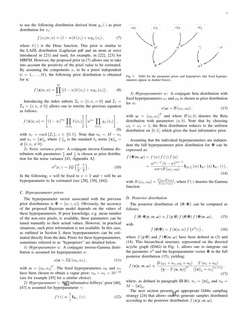
The hyperparameter vector associated with the previousprior distributions is Φ = {a, γ, w}. Obviously, the accuracyof the proposed Bayesian model depends on the values ofthese hyperparameters. If prior knowledge, e.g. mean numberof the non-zero pixels, is available, these parameters can betuned manually to their actual values. However, in practicalsituations, such prior information is not available. In this case,as outlined in Section I, these hyperparameters can be esti-mated directly from the data. Priors for these hyperparameters,sometimes referred to as “hyperpriors” are detailed below.

1) Hyperparameter a: A conjugate inverse-Gamma distri-bution is assumed for hyperparameter a:

a|α ∼ IG (α0, α1) , (11)

with α = [α0, α1]T . The fixed hyperparameters α0 and α1

have been chosen to obtain a vague prior: α0 = α1 = 10−10

(see for example [45] for a similar choice).2) Hyperparameter γ: Non informative Jeffreys’ prior [46],

[47] is assumed for hyperparameter γ:

f (γ) ∝ 1γ

1R+ (γ) . (12)

Fig. 1. DAG for the parameter priors and hyperpriors (the fixed hyperpa-rameters appear in dashed boxes).

3) Hyperparameter w: A conjugate beta distribution withfixed hyperparameters ω1 and ω0 is chosen as prior distributionfor w:

w|ω ∼ B (ω1, ω0) , (13)

with ω = [ω0, ω1]T and where B (a, b) denotes the Betadistribution with parameters (a, b). Note that by choosingω0 = ω1 = 1, the Beta distribution reduces to the uniformdistribution on [0, 1], which gives the least informative prior.

Assuming that the individual hyperparameters are indepen-dent the full hyperparameter prior distribution for Φ can beexpressed as:

f (Φ|α,ω) = f (w) f (γ) f (a)

=wω1−1 (1− w)ω0−1

awγB (ω1, ω0)1[0,1] (w) 1R+ (a) 1R+ (γ) ,

(14)

with B (ω1, ω0) = Γ(ω1)Γ(ω0)Γ(ω1+ω0) , where Γ(·) denotes the Gamma

function.

D. Posterior distribution

The posterior distribution of {θ,Φ} can be computed asfollows:

f (θ,Φ|y,α,ω) ∝ f (y|θ) f (θ|Φ) f (Φ|α,ω) , (15)

withf (θ|Φ) = f (x|a,w) f

(σ2|γ

), (16)

where f (y|θ) and f (Φ|α,ω) have been defined in (3) and(14). This hierarchical structure, represented on the directedacyclic graph (DAG) in Fig. 1, allows one to integrate outthe parameter σ2 and the hyperparameter vector Φ in the fullposterior distribution (15), yielding:

f (x|y,α,ω) ∝ B (ω1 + n1, ω0 + n0)

‖y − T (κ,x)‖PΓ (n1 + α0)

[‖x‖1 + α1]n1+α0.

(17)

where, as defined in paragraph III-B1, n1 = ‖x‖0 and n0 =M − ‖x‖0.

The next section presents an appropriate Gibbs samplingstrategy [24] that allows ones to generate samples distributedaccording to the posterior distribution f (x|y,α,ω).

1

2

Page: 3

Number: 1 Author: vmuser Subject: Replacement Text Date: 9/17/2008 12:58:20 PM A non Number: 2 Author: vmuser Subject: Cross-Out Date: 9/17/2008 12:58:24 PM

4

IV. A GIBBS SAMPLING STRATEGYFOR SPARSE IMAGE RECONSTRUCTION

We propose in this section a Gibbs sampling strategythat allows one to generate samples

{x(t)

}t=1,...

distributedaccording to the posterior distribution in (17). As simulatingdirectly according to (17) is a difficult task, it is muchmore convenient to generate samples distributed according tothe joint posterior f

(x, σ2|y,α,ω

). The main steps of this

algorithm are detailed in subsections IV-A and IV-B (see alsoAlgorithm 1 below).

ALGORITHM 1:

Gibbs sampling algorithm for sparse image reconstruction

• Initialization:– Sample parameter x(0) from pdf in (9),– Sample parameters σ2(0) from the pdf in (10),– Set t← 1,

• Iterations: for t = 1, 2, . . . , do1. Sample hyperparameter w(t) from the pdf in (19),2. Sample hyperparameter a(t) from the pdf in (20),3. For i = 1, . . . ,M , sample parameter x(t)

i from pdf in(21),

4. Sample parameter σ2(t) from the pdf in (24),5. Set t← t+ 1.

A. Generation of samples according to f(x∣∣σ2,y,α,ω

)To generate samples distributed according to

f(x∣∣σ2,y,ω

), it is very convenient to sample according to

f(x, w, a

∣∣σ2,y,ω)

in the following 3-step procedure.1) Generation of samples according to f (w |x,ω ): Using

(9), the following result can be obtained:

f (w |x,ω ) ∝ (1− w)n0+ω0−1wn1+ω1−1, (18)

where n0 and n1 have been defined in paragraph III-B1.Therefore, generation of samples according to f (w |x,ω ) isachieved as follows:

w |x,ω ∼ Be (ω1 + n1, ω0 + n0) . (19)

2) Generation of samples according to f (a |x,α ): Look-ing at the joint posterior distribution (15), it yields:

a |x,α ∼ IG (‖x‖0 + α0, ‖x‖1 + α1) . (20)

3) Generation of samples according to f(x∣∣w, a, σ2,y

):

The prior chosen for xi (i = 1, . . . ,M ) yields a poste-rior distribution of x that is not closed form. However, theposterior distribution of each component xi (i = 1, . . . ,M )conditionally upon the others can be easily derived. Indeedstraightforward computations detailed in Appendix A yield:

f(xi|w, a, σ2,x−i,y

)∝ (1− wi)δ (xi)

+ wiφ+

(xi|µi, η2

i

),

(21)

where x−i stands for the vector x whose ith component hasbeen removed and µi and η2

i are given in Appendix A. In

(21), φ+

(·,m, s2

)stands for the pdf of the truncated Gaussian

distribution defined on R∗+ with hidden parameters equal tomean m and variance s2:

φ+

(x,m, s2

)=

1C (m, s2)

exp

[− (x−m)2

2s2

]1R∗+ (x) ,

(22)with

C(m, s2

)=

√πs2

2

[1 + erf

(m√2s2

)]. (23)

The form in (21) specifies xi|w, a, σ2,x−i,y as a Bernoulli-truncated Gaussian variable with parameter

(wi, µi, η

2i

). Ap-

pendix C presents an algorithm that can be used to generatesamples distributed according to this distribution.

To summarize, generating samples distributed according tof(x∣∣w, σ2, a, ,y

)can be performed by updating the coor-

dinates of x successively using M Gibbs moves (requiringgeneration of Bernoulli-truncated Gaussian variables).

B. Generation of samples according to f(σ2 |x,y

)Samples are generated as the following way:

σ2 |x,y ∼ IG

(P

2,‖y − T (κ,x)‖2

2

). (24)

V. SIMULATION ON SYNTHETIC IMAGES

TABLE IPARAMETERS USED TO COMPUTE THE MRFM PSF.

ParameterValue

Description Name

Amplitude of external magnetic field Bext 9.4× 103 G

Value of Bmag in the resonant slice Bres 1.0× 104 G

Radius of tip R0 4.0 nm

Distance from tip to sample d 6.0 nm

Cantilever tip moment m 4.6× 105 emu

Peak cantilever oscillation oscillation xpk 0.8 nm

Maximum magnetic field gradient Gmax 125

Fig. 2. Left: Psf of the MRFM tip. Right: unknown sparse image to beestimated.

1 2

3 4

5

Page: 4

Number: 1 Author: vmuser Subject: Replacement Text Date: 9/17/2008 12:58:34 PM In Number: 2 Author: vmuser Subject: Inserted Text Date: 9/17/2008 12:58:36 PM we describe the Number: 3 Author: vmuser Subject: Replacement Text Date: 9/17/2008 12:58:41 PM for Number: 4 Author: vmuser Subject: Replacement Text Date: 9/17/2008 12:58:44 PM generating Number: 5 Author: vmuser Subject: Replacement Text Date: 9/17/2008 12:58:54 PM from

5

A. Reconstruction of 2-dimensional imageIn this subsection, a 32 × 32 synthetic image, depicted in

Fig. 2 (right), is simulated using the prior in (9) with parametera = 1 and w = 0.02. In this figure and in the followingones, white pixels stands for identically null values. A generalanalytical derivation of the psf of the MRFM tip has beengiven in [39] and is explained in [23]. Following this model,a 10 × 10 2-dimensional convolution kernel, represented inFig. 2 (left), has been generated when the physical parametersare tuned to the values gathered in Table I. The correspondingmatrix H introduced in (2) is of size 1024 × 1024. Theobserved measurements y, depicted in Fig. 2 (right) are of sizeP = 1024. These observations are corrupted by an additiveGaussian noise with two different variances σ2 = 1.2× 10−1

and σ2 = 1.6× 10−3, corresponding to signal-to-noise ratiosSNR = 2dB and SNR = 20dB respectively.

1) Simulation results: The observations are processed bythe proposed algorithm that consists of NMC = 2000 iterationsof the Gibbs sampler with Nbi = 300 burn-in iterations. Thenthe MAP estimator of the unknown image x is computed bykeeping among X =

{x(t)

}t=1,...,NMC

the generated samplethat maximizes the posterior distribution in (17):

xMAP = argmaxx∈RM

+

f (x|y)

≈ argmaxx∈X

f (x|y) .(25)

These estimates are depicted in Fig. 3 for the two levels ofnoise considered. It can be noticed that the estimated imageis very similar to the actual image, even with a low SNR.

Fig. 3. Top, left (resp. right): noisy observations for SNR = 2dB (resp.20dB). Bottom, left (resp. right): reconstructed image for SNR = 2dB (resp.20dB).

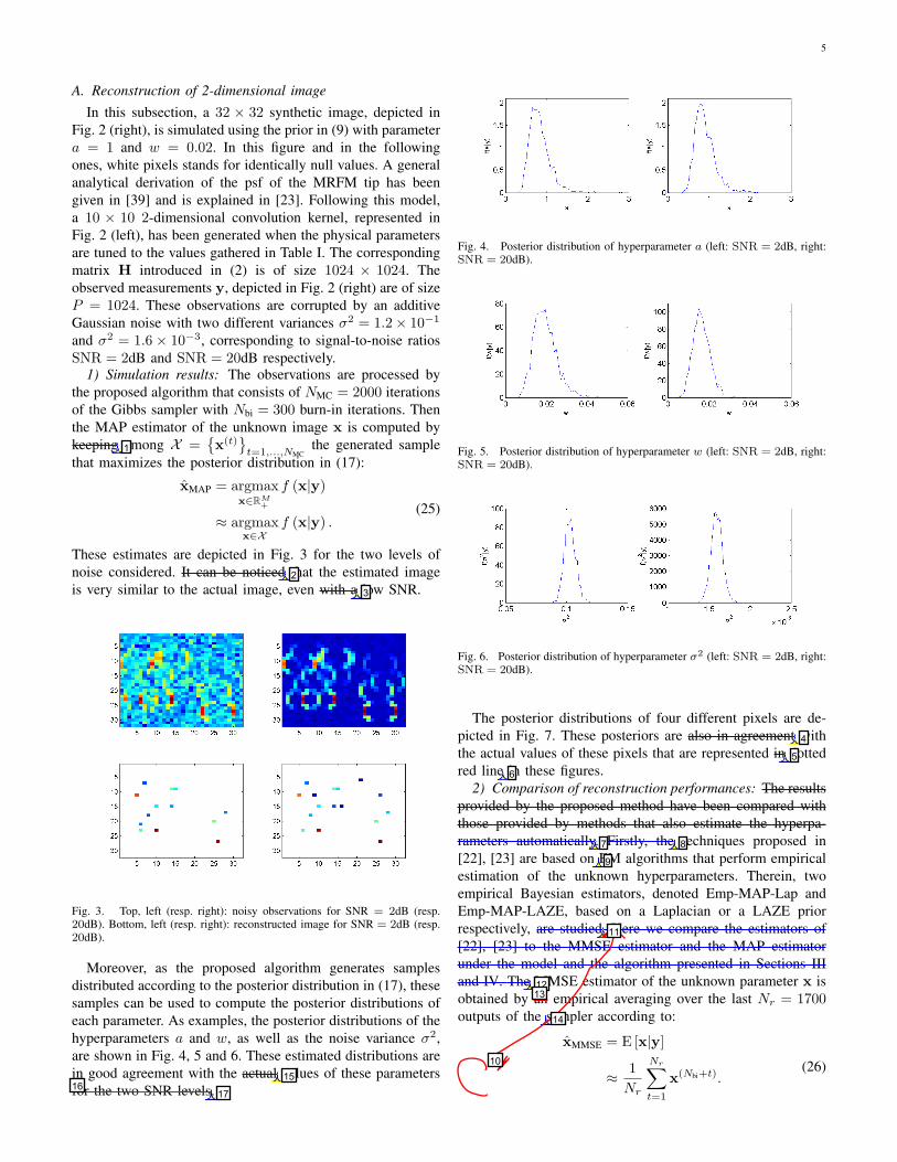
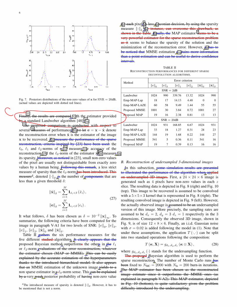
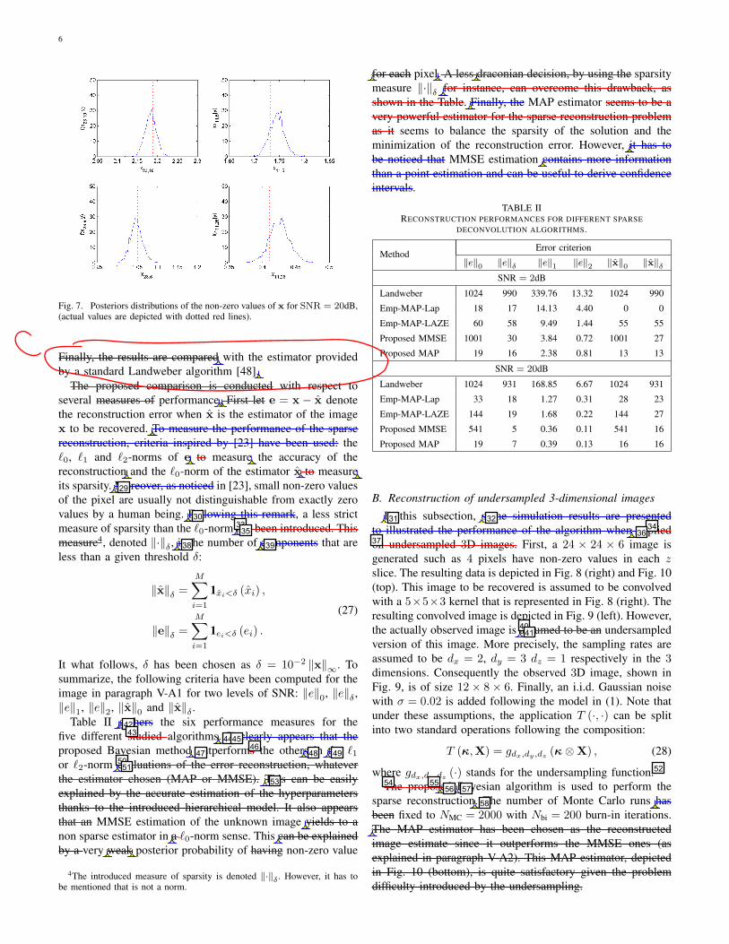
Moreover, as the proposed algorithm generates samplesdistributed according to the posterior distribution in (17), thesesamples can be used to compute the posterior distributions ofeach parameter. As examples, the posterior distributions of thehyperparameters a and w, as well as the noise variance σ2,are shown in Fig. 4, 5 and 6. These estimated distributions arein good agreement with the actual values of these parametersfor the two SNR levels.

Fig. 4. Posterior distribution of hyperparameter a (left: SNR = 2dB, right:SNR = 20dB).

Fig. 5. Posterior distribution of hyperparameter w (left: SNR = 2dB, right:SNR = 20dB).

Fig. 6. Posterior distribution of hyperparameter σ2 (left: SNR = 2dB, right:SNR = 20dB).

The posterior distributions of four different pixels are de-picted in Fig. 7. These posteriors are also in agreement withthe actual values of these pixels that are represented in dottedred line in these figures.

2) Comparison of reconstruction performances: The resultsprovided by the proposed method have been compared withthose provided by methods that also estimate the hyperpa-rameters automatically. Firstly, the techniques proposed in[22], [23] are based on EM algorithms that perform empiricalestimation of the unknown hyperparameters. Therein, twoempirical Bayesian estimators, denoted Emp-MAP-Lap andEmp-MAP-LAZE, based on a Laplacian or a LAZE priorrespectively, are studied. Here we compare the estimators of[22], [23] to the MMSE estimator and the MAP estimatorunder the model and the algorithm presented in Sections IIIand IV. The MMSE estimator of the unknown parameter x isobtained by an empirical averaging over the last Nr = 1700outputs of the sampler according to:

xMMSE = E [x|y]

≈ 1Nr

Nr∑t=1

x(Nbi+t).(26)

1

2

3

4

5

6

7 8

9

10

11

1213

14

1516

17

Page: 5

Number: 1 Author: vmuser Subject: Replacement Text Date: 9/17/2008 12:59:00 PM retaining Number: 2 Author: vmuser Subject: Replacement Text Date: 9/17/2008 12:59:11 PM Observe Number: 3 Author: vmuser Subject: Replacement Text Date: 9/17/2008 12:59:14 PM at Number: 4 Author: vmuser Subject: Replacement Text Date: 9/17/2008 12:59:44 PM consistent Number: 5 Author: vmuser Subject: Replacement Text Date: 9/17/2008 12:59:47 PM as Number: 6 Author: vmuser Subject: Inserted Text Date: 9/17/2008 12:59:48 PM s Number: 7 Author: vmuser Subject: Replacement Text Date: 9/17/2008 1:00:42 PM Here we compare our proposed hierarchical Bayesian method to the methods of [22],[23]. Number: 8 Author: vmuser Subject: Replacement Text Date: 9/17/2008 1:00:17 PM The Number: 9 Author: vmuser Subject: Inserted Text Date: 9/17/2008 1:00:24 PM penalized likelihood Number: 10 Author: vmuser Subject: Pencil Date: 9/17/2008 1:03:10 PM Number: 11 Author: vmuser Subject: Replacement Text Date: 9/17/2008 1:01:10 PM were proposed. Number: 12 Author: vmuser Subject: Replacement Text Date: 9/17/2008 1:02:23 PM These will be compared to our hierarchical Bayesian MAP estimator, given in (25), and also to a minimum mean square error (MMSE) estimator extracted from the estimated fullBayes posterior (17). The Number: 13 Author: vmuser Subject: Cross-Out Date: 9/17/2008 1:02:25 PM Number: 14 Author: vmuser Subject: Inserted Text Date: 9/17/2008 1:02:28 PM Gibbs Number: 15 Author: vmuser Subject: Replacement Text Date: 9/17/2008 12:59:21 PM ground truth Number: 16 Author: vmuser Subject: Cross-Out Date: 9/17/2008 12:59:31 PM Number: 17 Author: vmuser Subject: Inserted Text Date: 9/17/2008 12:59:30 PM ; randomly drawn from the prior distribution

6

Fig. 7. Posteriors distributions of the non-zero values of x for SNR = 20dB,(actual values are depicted with dotted red lines).

Finally, the results are compared with the estimator providedby a standard Landweber algorithm [48].

The proposed comparison is conducted with respect toseveral measures of performance. First let e = x − x denotethe reconstruction error when x is the estimator of the imagex to be recovered. To measure the performance of the sparsereconstruction, criteria inspired by [23] have been used: the`0, `1 and `2-norms of e to measure the accuracy of thereconstruction and the `0-norm of the estimator x to measureits sparsity. Moreover, as noticed in [23], small non-zero valuesof the pixel are usually not distinguishable from exactly zerovalues by a human being. Following this remark, a less strictmeasure of sparsity than the `0-norm has been introduced. Thismeasure4, denoted ‖·‖δ , is the number of components that areless than a given threshold δ:

‖x‖δ =M∑i=1

1xi<δ (xi) ,

‖e‖δ =M∑i=1

1ei<δ (ei) .

(27)

It what follows, δ has been chosen as δ = 10−2 ‖x‖∞. Tosummarize, the following criteria have been computed for theimage in paragraph V-A1 for two levels of SNR: ‖e‖0, ‖e‖δ ,‖e‖1, ‖e‖2, ‖x‖0 and ‖x‖δ .

Table II gathers the six performance measures for thefive different studied algorithms. It clearly appears that theproposed Bayesian method outperforms the others in the `1or `2-norm evaluations of the error reconstruction, whateverthe estimator chosen (MAP or MMSE). This can be easilyexplained by the accurate estimation of the hyperparametersthanks to the introduced hierarchical model. It also appearsthat an MMSE estimation of the unknown image yields to anon sparse estimator in a `0-norm sense. This can be explainedby a very weak posterior probability of having non-zero value

4The introduced measure of sparsity is denoted ‖·‖δ . However, it has tobe mentioned that is not a norm.

for each pixel. A less draconian decision, by using the sparsitymeasure ‖·‖δ for instance, can overcome this drawback, asshown in the Table. Finally, the MAP estimator seems to be avery powerful estimator for the sparse reconstruction problemas it seems to balance the sparsity of the solution and theminimization of the reconstruction error. However, it has tobe noticed that MMSE estimation contains more informationthan a point estimation and can be useful to derive confidenceintervals.

TABLE IIRECONSTRUCTION PERFORMANCES FOR DIFFERENT SPARSE

DECONVOLUTION ALGORITHMS.

MethodError criterion

‖e‖0 ‖e‖δ ‖e‖1 ‖e‖2 ‖x‖0 ‖x‖δSNR = 2dB

Landweber 1024 990 339.76 13.32 1024 990

Emp-MAP-Lap 18 17 14.13 4.40 0 0

Emp-MAP-LAZE 60 58 9.49 1.44 55 55

Proposed MMSE 1001 30 3.84 0.72 1001 27

Proposed MAP 19 16 2.38 0.81 13 13

SNR = 20dB

Landweber 1024 931 168.85 6.67 1024 931

Emp-MAP-Lap 33 18 1.27 0.31 28 23

Emp-MAP-LAZE 144 19 1.68 0.22 144 27

Proposed MMSE 541 5 0.36 0.11 541 16

Proposed MAP 19 7 0.39 0.13 16 16

B. Reconstruction of undersampled 3-dimensional images

In this subsection, some simulation results are presentedto illustrated the performance of the algorithm when appliedon undersampled 3D images. First, a 24 × 24 × 6 image isgenerated such as 4 pixels have non-zero values in each zslice. The resulting data is depicted in Fig. 8 (right) and Fig. 10(top). This image to be recovered is assumed to be convolvedwith a 5×5×3 kernel that is represented in Fig. 8 (right). Theresulting convolved image is depicted in Fig. 9 (left). However,the actually observed image is assumed to be an undersampledversion of this image. More precisely, the sampling rates areassumed to be dx = 2, dy = 3 dz = 1 respectively in the 3dimensions. Consequently the observed 3D image, shown inFig. 9, is of size 12× 8× 6. Finally, an i.i.d. Gaussian noisewith σ = 0.02 is added following the model in (1). Note thatunder these assumptions, the application T (·, ·) can be splitinto two standard operations following the composition:

T (κ,X) = gdx,dy,dz(κ⊗X) , (28)

where gdx,dy,dz (·) stands for the undersampling function.The proposed Bayesian algorithm is used to perform the

sparse reconstruction. The number of Monte Carlo runs hasbeen fixed to NMC = 2000 with Nbi = 200 burn-in iterations.The MAP estimator has been chosen as the reconstructedimage estimate since it outperforms the MMSE ones (asexplained in paragraph V-A2). This MAP estimator, depictedin Fig. 10 (bottom), is quite satisfactory given the problemdifficulty introduced by the undersampling.

12 3 4

56

78

9

10

1112

1314

15

16 171819

20

2122 23

24252627 28

Page: 6

Number: 1 Author: vmuser Subject: Cross-Out Date: 9/17/2008 1:06:34 PM Number: 2 Author: vmuser Subject: Replacement Text Date: 9/17/2008 1:06:25 PM at many Number: 3 Author: vmuser Subject: Inserted Text Date: 9/17/2008 1:06:25 PM s Number: 4 Author: vmuser Subject: Inserted Text Date: 9/17/2008 1:06:38 PM The Number: 5 Author: vmuser Subject: Cross-Out Date: 9/17/2008 1:06:42 PM Number: 6 Author: vmuser Subject: Inserted Text Date: 9/17/2008 1:06:53 PM indicates that most of the pixels are in fact very close to zero. Number: 7 Author: vmuser Subject: Cross-Out Date: 9/17/2008 1:07:06 PM Number: 8 Author: vmuser Subject: Replacement Text Date: 9/17/2008 1:07:02 PM The Number: 9 Author: vmuser Subject: Replacement Text Date: 9/17/2008 1:07:28 PM by construction the Number: 10 Author: vmuser Subject: Replacement Text Date: 9/17/2008 1:07:42 PM will always have lower mean square error Number: 11 Author: vmuser Subject: Pencil Date: 9/17/2008 1:02:56 PM Number: 12 Author: vmuser Subject: Replacement Text Date: 9/17/2008 1:02:50 PM We also compare

Number: 13 Author: vmuser Subject: Cross-Out Date: 9/17/2008 1:03:24 PM Number: 14 Author: vmuser Subject: Inserted Text Date: 9/17/2008 1:03:33 PM As in [23] we compare estimators Number: 15 Author: vmuser Subject: Cross-Out Date: 9/17/2008 1:03:24 PM Number: 16 Author: vmuser Subject: Cross-Out Date: 9/17/2008 1:03:34 PM Number: 17 Author: vmuser Subject: Cross-Out Date: 9/17/2008 1:03:40 PM Number: 18 Author: vmuser Subject: Inserted Text Date: 9/17/2008 1:03:38 PM criteria Number: 19 Author: vmuser Subject: Inserted Text Date: 9/17/2008 1:03:42 PM Let Number: 20 Author: vmuser Subject: Replacement Text Date: 9/17/2008 1:03:53 PM These criteria are: Number: 21 Author: vmuser Subject: Cross-Out Date: 9/17/2008 1:03:56 PM Number: 22 Author: vmuser Subject: Inserted Text Date: 9/17/2008 1:03:55 PM , which Number: 23 Author: vmuser Subject: Inserted Text Date: 9/17/2008 1:04:06 PM s Number: 24 Author: vmuser Subject: Cross-Out Date: 9/17/2008 1:04:01 PM Number: 25 Author: vmuser Subject: Cross-Out Date: 9/17/2008 1:04:00 PM Number: 26 Author: vmuser Subject: Inserted Text Date: 9/17/2008 1:04:04 PM , which Number: 27 Author: vmuser Subject: Inserted Text Date: 9/17/2008 1:03:57 PM , Number: 28 Author: vmuser Subject: Inserted Text Date: 9/17/2008 1:04:04 PM s


6




‖x‖δ =M∑i=1

1xi<δ (xi) ,

‖e‖δ =M∑i=1

1ei<δ (ei) .

(27)








‖e‖0 ‖e‖δ ‖e‖1 ‖e‖2 ‖x‖0 ‖x‖δSNR = 2dB

Landweber 1024 990 339.76 13.32 1024 990

Emp-MAP-Lap 18 17 14.13 4.40 0 0

Emp-MAP-LAZE 60 58 9.49 1.44 55 55

Proposed MMSE 1001 30 3.84 0.72 1001 27

Proposed MAP 19 16 2.38 0.81 13 13

SNR = 20dB

Landweber 1024 931 168.85 6.67 1024 931

Emp-MAP-Lap 33 18 1.27 0.31 28 23

Emp-MAP-LAZE 144 19 1.68 0.22 144 27

Proposed MMSE 541 5 0.36 0.11 541 16

Proposed MAP 19 7 0.39 0.13 16 16



T (κ,X) = gdx,dy,dz(κ⊗X) , (28)



29

30 31 3233 3435 36

3738 39

4041

4243

444546

47 48 4950

51 5253 54 55

56 57

58

Number: 29 Author: vmuser Subject: Replacement Text Date: 9/17/2008 1:04:14 PM As pointed out Number: 30 Author: vmuser Subject: Replacement Text Date: 9/17/2008 1:04:10 PM Thus Number: 31 Author: vmuser Subject: Inserted Text Date: 9/17/2008 1:08:43 PM As iscussed in Sec. VI, the prototype MRFM instrument collects data projections as irregularly spaced, or undersampled, spatial samples. Number: 32 Author: vmuser Subject: Replacement Text Date: 9/17/2008 1:09:11 PM we indicate how the image reconstruction algorithm can be adapted to this undersampled scenario in 3D. Number: 33 Author: vmuser Subject: Cross-Out Date: 9/17/2008 1:04:25 PM Number: 34 Author: vmuser Subject: Cross-Out Date: 9/17/2008 1:09:13 PM Number: 35 Author: vmuser Subject: Inserted Text Date: 9/17/2008 1:04:26 PM , Number: 36 Author: vmuser Subject: Inserted Text Date: 9/17/2008 1:09:24 PM For concreteness, we illustrate by a concrete example. Number: 37 Author: vmuser Subject: Cross-Out Date: 9/17/2008 1:09:13 PM Number: 38 Author: vmuser Subject: Replacement Text Date: 9/17/2008 1:04:33 PM which is Number: 39 Author: vmuser Subject: Replacement Text Date: 9/17/2008 1:04:43 PM reconstructed image pixels Number: 40 Author: vmuser Subject: Cross-Out Date: 9/17/2008 1:09:28 PM Number: 41 Author: vmuser Subject: Inserted Text Date: 9/17/2008 1:09:31 PM an Number: 42 Author: vmuser Subject: Replacement Text Date: 9/17/2008 1:04:49 PM shows Number: 43 Author: vmuser Subject: Cross-Out Date: 9/17/2008 1:04:51 PM Number: 44 Author: vmuser Subject: Inserted Text Date: 9/17/2008 1:04:59 PM studied Number: 45 Author: vmuser Subject: Replacement Text Date: 9/17/2008 1:05:03 PM The Number: 46 Author: vmuser Subject: Cross-Out Date: 9/17/2008 1:05:15 PM Number: 47 Author: vmuser Subject: Inserted Text Date: 9/17/2008 1:05:14 PM s (labeled "proposed MMSE" and "proposed MAP" in the table)

Number: 48 Author: vmuser Subject: Replacement Text Date: 9/17/2008 1:05:19 PM estimators Number: 49 Author: vmuser Subject: Replacement Text Date: 9/17/2008 1:05:28 PM terms of Number: 50 Author: vmuser Subject: Cross-Out Date: 9/17/2008 1:05:31 PM Number: 51 Author: vmuser Subject: Inserted Text Date: 9/17/2008 1:05:35 PM s Number: 52 Author: vmuser Subject: Cross-Out Date: 9/17/2008 1:09:50 PM Number: 53 Author: vmuser Subject: Replacement Text Date: 9/17/2008 1:05:50 PM Note that the Number: 54 Author: vmuser Subject: Cross-Out Date: 9/17/2008 1:10:24 PM Number: 55 Author: vmuser Subject: Cross-Out Date: 9/17/2008 1:10:24 PM Number: 56 Author: vmuser Subject: Inserted Text Date: 9/17/2008 1:10:30 PM For illustration the proposed Number: 57 Author: vmuser Subject: Inserted Text Date: 9/17/2008 1:09:43 PM hierarchical Number: 58 Author: vmuser Subject: Inserted Text Date: 9/17/2008 1:10:37 PM with undersampled data


6




‖x‖δ =M∑i=1

1xi<δ (xi) ,

‖e‖δ =M∑i=1

1ei<δ (ei) .

(27)








‖e‖0 ‖e‖δ ‖e‖1 ‖e‖2 ‖x‖0 ‖x‖δSNR = 2dB

Landweber 1024 990 339.76 13.32 1024 990

Emp-MAP-Lap 18 17 14.13 4.40 0 0

Emp-MAP-LAZE 60 58 9.49 1.44 55 55

Proposed MMSE 1001 30 3.84 0.72 1001 27

Proposed MAP 19 16 2.38 0.81 13 13

SNR = 20dB

Landweber 1024 931 168.85 6.67 1024 931

Emp-MAP-Lap 33 18 1.27 0.31 28 23

Emp-MAP-LAZE 144 19 1.68 0.22 144 27

Proposed MMSE 541 5 0.36 0.11 541 16

Proposed MAP 19 7 0.39 0.13 16 16



T (κ,X) = gdx,dy,dz(κ⊗X) , (28)



59

6061

6263 6465 66

6768 69

Number: 59 Author: vmuser Subject: Replacement Text Date: 9/17/2008 1:10:40 PM was Number: 60 Author: vmuser Subject: Cross-Out Date: 9/17/2008 1:05:44 PM Number: 61 Author: vmuser Subject: Replacement Text Date: 9/17/2008 1:05:55 PM is a Number: 62 Author: vmuser Subject: Cross-Out Date: 9/17/2008 1:05:55 PM Number: 63 Author: vmuser Subject: Cross-Out Date: 9/17/2008 1:05:55 PM Number: 64 Author: vmuser Subject: Replacement Text Date: 9/17/2008 1:11:18 PM Figure 10 shows the result of applying the proposed MAP estimator to the estimated posterior. Number: 65 Author: vmuser Subject: Inserted Text Date: 9/17/2008 1:05:57 PM the Number: 66 Author: vmuser Subject: Replacement Text Date: 9/17/2008 1:06:05 PM is due to the Number: 67 Author: vmuser Subject: Cross-Out Date: 9/17/2008 1:06:14 PM Number: 68 Author: vmuser Subject: Replacement Text Date: 9/17/2008 1:06:11 PM small Number: 69 Author: vmuser Subject: Inserted Text Date: 9/17/2008 1:06:08 PM but non-zero

7

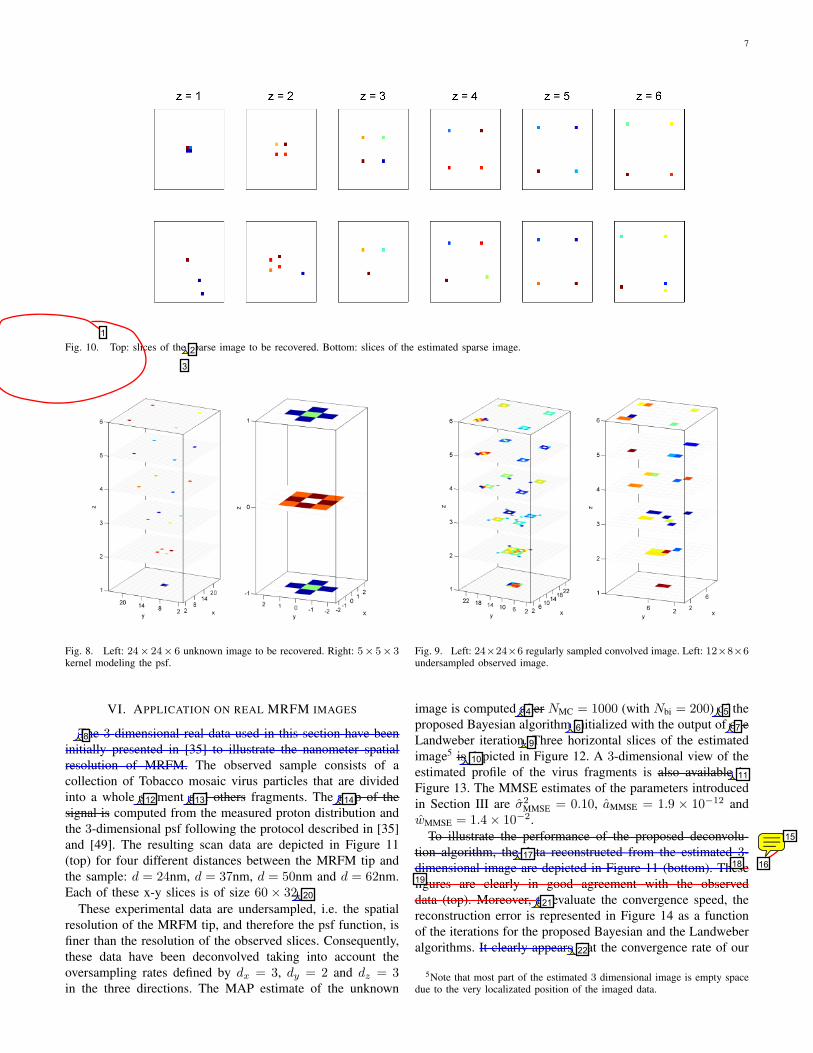
Fig. 10. Top: slices of the sparse image to be recovered. Bottom: slices of the estimated sparse image.

Fig. 8. Left: 24× 24× 6 unknown image to be recovered. Right: 5× 5× 3kernel modeling the psf.

VI. APPLICATION ON REAL MRFM IMAGES

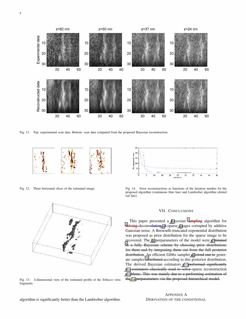
The 3-dimensional real data used in this section have beeninitially presented in [35] to illustrate the nanometer spatialresolution of MRFM. The observed sample consists of acollection of Tobacco mosaic virus particles that are dividedinto a whole segment and others fragments. The map of thesignal is computed from the measured proton distribution andthe 3-dimensional psf following the protocol described in [35]and [49]. The resulting scan data are depicted in Figure 11(top) for four different distances between the MRFM tip andthe sample: d = 24nm, d = 37nm, d = 50nm and d = 62nm.Each of these x-y slices is of size 60× 32.

These experimental data are undersampled, i.e. the spatialresolution of the MRFM tip, and therefore the psf function, isfiner than the resolution of the observed slices. Consequently,these data have been deconvolved taking into account theoversampling rates defined by dx = 3, dy = 2 and dz = 3in the three directions. The MAP estimate of the unknown

Fig. 9. Left: 24×24×6 regularly sampled convolved image. Left: 12×8×6undersampled observed image.

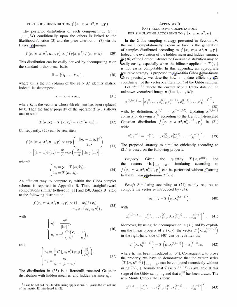
image is computed after NMC = 1000 (with Nbi = 200) of theproposed Bayesian algorithm initialized with the output of oneLandweber iteration. Three horizontal slices of the estimatedimage5 is depicted in Figure 12. A 3-dimensional view of theestimated profile of the virus fragments is also available inFigure 13. The MMSE estimates of the parameters introducedin Section III are σ2

MMSE = 0.10, aMMSE = 1.9 × 10−12 andwMMSE = 1.4× 10−2.

To illustrate the performance of the proposed deconvolu-tion algorithm, the data reconstructed from the estimated 3-dimensional image are depicted in Figure 11 (bottom). Thesefigures are clearly in good agreement with the observeddata (top). Moreover, to evaluate the convergence speed, thereconstruction error is represented in Figure 14 as a functionof the iterations for the proposed Bayesian and the Landweberalgorithms. It clearly appears that the convergence rate of our

5Note that most part of the estimated 3 dimensional image is empty spacedue to the very localizated position of the imaged data.

1

2

3

4 5

6 78

9

10

11

12 13 14

15

1617

18

19

2021

22

Page: 7

Number: 1 Author: vmuser Subject: Pencil Date: 9/17/2008 1:14:57 PM Number: 2 Author: vmuser Subject: Inserted Text Date: 9/17/2008 1:15:12 PM This figure is out of order! Number: 3 Author: vmuser Subject: Typewritten Text Date: 9/17/2008 1:15:03 PM Number: 4 Author: vmuser Subject: Replacement Text Date: 9/17/2008 1:13:31 PM from Number: 5 Author: vmuser Subject: Inserted Text Date: 9/17/2008 1:13:34 PM Gibbs samples Number: 6 Author: vmuser Subject: Inserted Text Date: 9/17/2008 1:13:38 PM . The algorithm was Number: 7 Author: vmuser Subject: Replacement Text Date: 9/17/2008 1:13:41 PM a single Number: 8 Author: vmuser Subject: Replacement Text Date: 9/17/2008 1:13:02 PM Here we illustrate the heirarchical Bayes MAP reconstruction algorithm for real lthree dimensional MRFM data. The data is a set of MRFM projections of a sample of tobacco virus. Comprehensive details of both the experiment and the MRFM data acquisition protocol are given in [35]. Number: 9 Author: vmuser Subject: Inserted Text Date: 9/17/2008 1:14:44 PM Several more iterations of the Landweber algorithm would produce the reconstructions reported in [35]. Theimage reconstructions produced by the Landweber and Bayesian MAP algorithm are shown in Figs. 11-13. Number: 10 Author: vmuser Subject: Replacement Text Date: 9/17/2008 1:15:31 PM are Number: 11 Author: vmuser Subject: Replacement Text Date: 9/17/2008 1:15:35 PM shown Number: 12 Author: vmuser Subject: Inserted Text Date: 9/17/2008 1:12:49 PM viral Number: 13 Author: vmuser Subject: Replacement Text Date: 9/17/2008 1:12:47 PM in addiiton to viral Number: 14 Author: vmuser Subject: Replacement Text Date: 9/17/2008 1:13:09 PM projections are Number: 15 Author: vmuser Subject: Sticky Note Date: 9/17/2008 1:17:29 PM Nicolas - pourras-tu mettre une troisieme serie d'images pour comparer Bayes contre Landweber dans Fig 11? Number: 16 Author: vmuser Subject: Pencil Date: 9/17/2008 1:17:09 PM Number: 17 Author: vmuser Subject: Replacement Text Date: 9/17/2008 1:16:38 PM By forward projecting the estimated virus image through the point spread function one can visually evaluate the goodness of fit of the reconstruction to the raw measured data. This is depicted in Fig. 11. Number: 18 Author: vmuser Subject: Cross-Out Date: 9/17/2008 1:16:58 PM Number: 19 Author: vmuser Subject: Cross-Out Date: 9/17/2008 1:16:57 PM Number: 20 Author: vmuser Subject: Inserted Text Date: 9/17/2008 1:13:21 PM pixels Number: 21 Author: vmuser Subject: Replacement Text Date: 9/17/2008 1:17:01 PM To Number: 22 Author: vmuser Subject: Replacement Text Date: 9/17/2008 1:17:48 PM This shows

8

Fig. 11. Top: experimental scan data. Bottom: scan data computed from the proposed Bayesian reconstruction.

Fig. 12. Three horizontal slices of the estimated image.

Fig. 13. 3-dimensional view of the estimated profile of the Tobacco virusfragments.

algorithm is significantly better than the Landweber algorithm.

Fig. 14. Error reconstructions as functions of the iteration number for theproposed algorithm (continuous blue line) and Landweber algorithm (dottedred line).

VII. CONCLUSIONS

This paper presented a Bayesian sampling algorithm forsolving deconvolution of sparse images corrupted by additiveGaussian noise. A Bernoulli-truncated exponential distributionwas proposed as prior distribution for the sparse image to berecovered. The hyperparameters of the model were estimatedin a fully Bayesian scheme by choosing prior distributionsfor them and by integrating them out from the full posteriordistribution. An efficient Gibbs sampler allowed one to gener-ate samples distributed according to this posterior distribution.The derived Bayesian estimators outperformed significantlythe estimators classically used to solve sparse reconstructionproblems. This was mainly due to a performing estimation ofthe hyperparameters via the proposed hierarchical model.

APPENDIX ADERIVATION OF THE CONDITIONAL

12

34 5

6 78

910

11

12

13

14

Page: 8

Number: 1 Author: vmuser Subject: Cross-Out Date: 9/17/2008 1:18:00 PM Number: 2 Author: vmuser Subject: Inserted Text Date: 9/17/2008 1:17:58 PM hierarchical Number: 3 Author: vmuser Subject: Cross-Out Date: 9/17/2008 1:18:02 PM Number: 4 Author: vmuser Subject: Replacement Text Date: 9/17/2008 1:18:04 PM ing Number: 5 Author: vmuser Subject: Inserted Text Date: 9/17/2008 1:18:10 PM positive Number: 6 Author: vmuser Subject: Inserted Text Date: 9/17/2008 1:18:26 PM unknown Number: 7 Author: vmuser Subject: Replacement Text Date: 9/17/2008 1:19:22 PM integrated out of the posterior distribution of the image producing a full posterior distribution that can be used for estimation of the pixel values by maximization (MAP) or integration (MMSE). Number: 8 Author: vmuser Subject: Cross-Out Date: 9/17/2008 1:19:25 PM Number: 9 Author: vmuser Subject: Replacement Text Date: 9/17/2008 1:19:29 PM was used to Number: 10 Author: vmuser Subject: Cross-Out Date: 9/17/2008 1:19:31 PM Number: 11 Author: vmuser Subject: Replacement Text Date: 9/17/2008 1:19:37 PM significantly outperformed Number: 12 Author: vmuser Subject: Replacement Text Date: 9/17/2008 1:19:43 PM several previously proposed Number: 13 Author: vmuser Subject: Replacement Text Date: 9/17/2008 1:19:50 PM algorithms Number: 14 Author: vmuser Subject: Inserted Text Date: 9/17/2008 1:21:16 PM Our approach was implemented on real MRFM data to form a 3D image of a tobacco virus. Future work will include extension of the proposed method to other sparse bases, inclusion of uncertain point spread functions, and investigation of molecular priors.

9

POSTERIOR DISTRIBUTION f(xi∣∣w, a, σ2,x−i,y

)The posterior distribution of each component xi (i =

1, . . . ,M ) conditionally upon the others is linked to thelikelihood function (3) and the prior distribution (7) via theBayes’ paradigm:


)∝ f

(y|x, σ2

)f (xi|w, a) . (29)

This distribution can be easily derived by decomposing x onthe standard orthonormal basis

B = {u1, . . . ,uM} , (30)

where ui is the ith column of the M ×M identity matrix.Indeed, let decompose

x = xi + xiui, (31)

where xi is the vector x whose ith element has been replacedby 0. Then the linear property of the operator T (κ, ·) allowsone to state:

T (κ,x) = T (κ, xi) + xiT (κ,ui) . (32)

Consequently, (29) can be rewritten


)∝ exp

(−‖ei − xihi‖

2

2σ2

)×[(1− w)δ (xi) +

w

aexp

(−xia

)1R∗+ (xi)

],

(33)

where6 {ei = y − T (κ, xi) ,hi = T (κ,ui) .

(34)

An efficient way to compute ei within the Gibbs samplerscheme is reported in Appendix B. Then, straightforwardcomputations similar to those in [11] and [50, Annex B] yieldto the following distribution:


)∝ (1− wi)δ (xi)

+ wiφ+

(xi|µi, η2

i

),

(35)

with η2i =

σ2

‖hi‖2,

µi = η2i

(hTi eiσ2− 1a

),

(36)

and ui =

w

aC(µi, η

2i

)exp

(µ2i

2η2i

),

wi =ui

ui + (1− w).

(37)

The distribution in (35) is a Bernoulli-truncated Gaussiandistribution with hidden mean µi and hidden variance η2

i .

6It can be noticed that, for deblurring applications, hi is also the ith columnof the matrix H introduced in (2).

APPENDIX BFAST RECURSIVE COMPUTATIONS

FOR SIMULATING ACCORDING TO f(x∣∣w, a, σ2,y

)In the Gibbs sampling strategy presented in Section IV,

the main computationally expensive task is the generationof samples distributed according to f

(xi∣∣w, a, σ2,x−i,y

).

Indeed, the evaluation of the hidden mean and hidden variancein (36) of the Bernoulli-truncated Gaussian distribution may bereally costly, especially when the bilinear application T (·, ·)is not easily computable. In this appendix, an appropriaterecursive strategy is proposed to make this Gibbs move faster.More precisely, we describe how to update efficiently thecoordinate i of the vector x at iteration t of the Gibbs sampler.

Let x(t,i−1) denote the current Monte Carlo state of theunknown vectorized image x (i = 1, . . . ,M ):

x(t,i−1) =[x

(t)1 , . . . , x

(t)i−1, x

(t−1)i , x

(t−1)i+1 , . . . , x

(t−1)M

]T.

(38)with, by definition, x(t,0) = x(t−1,M). Updating x(t,i−1)

consists of drawing x(t)i according to the Bernoulli-truncated

Gaussian distribution f(xi

∣∣∣w, a, σ2,x(t,i−1)−i ,y

)in (21)

with:

x(t,i−1)−i =

[x

(t)1 , . . . , x

(t)i−1, x

(t−1)i+1 , . . . , x

(t−1)M

]T. (39)

The proposed strategy to simulate efficiently according to(21) is based on the following property.

Property: Given the quantity T(κ,x(0)

)and

the vectors {hi}i=1,...,M , simulating according to

f(xi

∣∣∣w, a, σ2,x(t,i)−i ,y

)can be performed without resorting

to the bilinear application T (·, ·).

Proof : Simulating according to (21) mainly requires tocompute the vector ei introduced by (34):

ei = y − T(κ, x(t,i−1)

i

), (40)

with

x(t,i−1)i =

[x

(t)1 , . . . , x

(t)i−1, 0, x

(t−1)i+1 , . . . , x

(t−1)M

]T. (41)

Moreover, by using the decomposition in (31) and by exploit-ing the linear property of T (κ, ·), the vector T

(κ, x(t,i−1)

i

)in the right-hand side of (40) can be rewritten as:

T(κ, x(t,i−1)

i

)= T

(κ,x(t,i−1)

)− x(t−1)

i hi, (42)

where hi has been introduced in (34). Consequently, to provethe property, we have to demonstrate that the vector series{T(κ,x(t,k)

)}k=1,...,M

can be computed recursively withoutusing T (·, ·). Assume that T

(κ,x(t,i−1)

)is available at this

stage of the Gibbs sampling and that x(t)i has been drawn. The

new Monte Carlo state is then:

x(t,i) =[x

(t)1 , . . . , x

(t)i−1, x

(t)i , x

(t−1)i+1 , . . . , x

(t−1)M

]T. (43)

1

2

3 45

6

7

8

Page: 9

Number: 1 Author: vmuser Subject: Replacement Text Date: 9/17/2008 1:21:23 PM formula Number: 2 Author: vmuser Subject: Cross-Out Date: 9/17/2008 1:21:25 PM Number: 3 Author: vmuser Subject: Replacement Text Date: 9/17/2008 1:21:32 PM accelerate the Number: 4 Author: vmuser Subject: Replacement Text Date: 9/17/2008 1:21:45 PM sampling by Number: 5 Author: vmuser Subject: Cross-Out Date: 9/17/2008 1:21:47 PM Number: 6 Author: vmuser Subject: Inserted Text Date: 9/17/2008 1:21:51 PM updating Number: 7 Author: vmuser Subject: Replacement Text Date: 9/17/2008 1:22:00 PM evaluating Number: 8 Author: vmuser Subject: Replacement Text Date: 9/17/2008 1:22:06 PM function

10

Similarly to (42), the vector T(κ,x(t,i)

)can be decomposed

as follows:

T(κ,x(t,i)

)= T

(κ, x(t,i−1)

i

)+ x

(t)i hi. (44)

Therefore, combining (42) and (44) allow one to state:

T(κ,x(t,i)

)= T

(κ,x(t,i−1)

)+(x

(t)i − x

(t−1)i

)hi.

�

As a conclusion, the bilinear application T (·, ·) has only tobe used at the very beginning of the algorithm to evaluateT(κ,x(0)

)and the vectors {hi}i=1,...,M . The resulting sim-

ulation scheme corresponding to step 3 of Algorithm 1 isdetailed in Algorithm 2.

ALGORITHM 2:

Efficient simulation according to f(x∣∣w, a, σ2,y

)For i = 1, . . . ,M, update the ith coordinate of the vector

x(t,i−1) =[x

(t)1 , . . . , x

(t)i−1, x

(t−1)i , x

(t−1)i+1 , . . . , x

(t−1)M

]Tvia the following steps:

1. compute ‖hi‖2,2. set T

(κ, x

(t,i−1)i

)= T

(κ,x(t,i−1)

)− x(t−1)

i hi,

3. set ei = x− T(κ, x

(t,i−1)i

),

4. compute µi, η2i and wi as defined in (36) and (37),

5. draw x(t)i according to (21),

6. set x(t,i) =[x

(t)1 , . . . , x

(t)i−1, x

(t)i , x

(t−1)i+1 , . . . , x

(t−1)M

]T,

7. set T(κ,x(t,i)

)= T

(κ, x

(t,i−1)i

)+ x

(t)i hi.

APPENDIX CSIMULATION ACCORDING TO A

BERNOULLI-TRUNCATED GAUSSIAN DISTRIBUTION

This appendix presents a general scheme to generate ran-dom variables distributed according to a Bernoulli-truncatedGaussian distribution with parameters

(w,m, s2

)whose pdf

is:

f(x|λ,m, s2

)= (1− λ) δ(x)

+λ

C (m, s2)exp

[− (x−m)2

2s2

]1R∗+ (x)

where C(m, s2

)has been defined in (23). This generation can

be conducted by using an auxiliary binary variable ε followingthe strategy detailed in Algorithm 3.

In the algorithm presented above, Ber (·) and N+ (·, ·)denote the Bernoulli and the positive truncated Gaussiandistributions respectively. In step 2, generation of samplesdistributed according to the truncated Gaussian distribution canbe achieved by using an appropriate accept-reject procedurewith different instrumental distributions [51]–[53].

ALGORITHM 3:

Simulation according toa Bernoulli-truncated Gaussian distribution

1. generate ε according to ε ∼ Ber (λ),

2. set{x = 0, if ε = 0;x ∼ N+

(m, s2

), if ε = 1.

ACKNOWLEDGEMENTS

The authors would like to thank M. Ting for providing thecode to generate point spread functions of MRFM tip and forinteresting suggestions regarding this work. The authors arealso very grateful to Dr. Dan Rugar who provided the realdata used in Section VIas well as a valuable feedback aboutthis paper.

REFERENCES

[1] H. Andrews and B. Hunt, Digital Image Restoration. Englewood Cliffs,NJ: Prentice-Hall, 1977.

[2] J. C. Russ, The image processing handbook, 5th ed. Boca Raton, FL:CRC Press, 2006.

[3] J.-L. Starck and F. Murtagh, Astronomical Image and Data Analysis,2nd ed. Berlin Heidelberg: Springer-Verlag, 2006.

[4] P. Sarder and A. Nehorai, “Deconvolution methods for 3-D fluorescencemicroscopy images,” IEEE Signal Processing Magazine, vol. 23, no. 3,pp. 32–45, May 2006.

[5] S. E. Reichenbach, D. E. Koehler, and D. W. Strelow, “Restoration andreconstruction of AVHRR images,” IEEE Trans. Geosci. and RemoteSensing, vol. 33, no. 4, pp. 997–1007, July 1995.

[6] F. Sroubek and J. Flusser, “Multichannel blind iterative image restora-tion,” IEEE Trans. Image Processing, vol. 12, no. 9, pp. 1094–1106,Sept. 2003.

[7] D. Mounce, “Magnetic resonance force microscopy,” IEEE Instr. Meas.Magazine, vol. 8, no. 2, pp. 20–26, June 2005.

[8] S. Kuehn, S. A. Hickman, and J. A. Marohn, “Advances in mechanicaldetection of magnetic resonance,” J. Chemical Physics, vol. 128, no. 5,Feb. 2008.

[9] D. Rugar, R. Budakian, H. J. Mamin, and B. W. Chui, “Single spindetection by magnetic resonance force microscopy,” Nature, vol. 430,pp. 329–332, July 2004.

[10] S. Bourguignon, H. Carfantan, and J. Idier, “A sparsity-based methodfor the estimation of spectral lines from irregularly sampled data,” IEEEJ. Sel. Topics Signal Processing, vol. 1, no. 4, Dec. 2007.

[11] Q. Cheng, R. Chen, and T.-H. Li, “Simultaneous wavelet estimation anddeconvolution of reflection seismic signals,” IEEE Trans. Geosci. andRemote Sensing, vol. 34, no. 2, pp. 377–384, March 1996.

[12] O. Rosec, J.-M. Boucher, B. Nsiri, and T. Chonavel, “Blind marine seis-mic deconvolution using statistical MCMC methods,” IEEE J. Ocean.Eng., vol. 28, no. 3, pp. 502–512, July 2003.

[13] T. Olofsson and E. Wennerstrom, “Sparse deconvolution of B-scanimages,” IEEE Trans. Ultrason. Ferroelectr. Freq. Control, vol. 54, no. 8,Aug. 2007.

[14] J. J. Kormylo and J. M. Mendel, “Maximum likelihood detection andestimation of Bernoulli-Gaussian processes,” IEEE Trans. Inf. Theory,vol. 28, no. 3, pp. 482–488, May 1982.

[15] J. Idier and Y. Goussard, “Stack algorithm for recursive deconvolution ofBernoulli-gaussian processes,” IEEE Trans. Signal Processing, vol. 28,no. 5, pp. 67–79, Sept. 1990.

[16] M. Lavielle, “Bayesian deconvolution of Bernoulli-Gaussian processes,”Signal Processing, vol. 33, no. 1, pp. 67–79, July 1993.

[17] F. Champagnat, Y. Goussard, and J. Idier, “Unsupervised deconvolutionof sparse spike trains using stochastic approximation,” IEEE Trans.Signal Processing, vol. 44, no. 12, pp. 2988–2998, Dec. 1996.

[18] A. Doucet and P. Duvaut, “Bayesian estimation of state-space modelsapplied to deconvolution of Bernoulli-Gaussian processes,” Signal Pro-cessing, vol. 57, no. 2, pp. 147–161, March 1997.

1 23 4 5

6

7

89

10

11

12

13

14

15

1617

Page: 10

Number: 1 Author: vmuser Subject: Cross-Out Date: 9/17/2008 1:22:14 PM Number: 2 Author: vmuser Subject: Cross-Out Date: 9/17/2008 1:22:22 PM Number: 3 Author: vmuser Subject: Replacement Text Date: 9/17/2008 1:22:17 PM The Number: 4 Author: vmuser Subject: Replacement Text Date: 9/17/2008 1:22:19 PM function Number: 5 Author: vmuser Subject: Inserted Text Date: 9/17/2008 1:22:25 PM needs Number: 6 Author: vmuser Subject: Inserted Text Date: 9/17/2008 1:22:28 PM Gibbs sampling Number: 7 Author: vmuser Subject: Cross-Out Date: 9/17/2008 1:22:30 PM Number: 8 Author: vmuser Subject: Pencil Date: 9/17/2008 1:23:40 PM Number: 9 Author: vmuser Subject: Replacement Text Date: 9/17/2008 1:22:39 PM shown Number: 10 Author: vmuser Subject: Sticky Note Date: 9/17/2008 1:23:55 PM Consider making Dan Rugar a co-author (I should be last on the list) Number: 11 Author: vmuser Subject: Replacement Text Date: 9/17/2008 1:22:50 PM describes how we Number: 12 Author: vmuser Subject: Replacement Text Date: 9/17/2008 1:23:09 PM Monte Carlo draws from this density can be obtained Number: 13 Author: vmuser Subject: Replacement Text Date: 9/17/2008 1:23:12 PM shown Number: 14 Author: vmuser Subject: Replacement Text Date: 9/17/2008 1:23:22 PM Algorithm 3 Number: 15 Author: vmuser Subject: Cross-Out Date: 9/17/2008 1:23:25 PM Number: 16 Author: vmuser Subject: Replacement Text Date: 9/17/2008 1:23:29 PM generated Number: 17 Author: vmuser Subject: Cross-Out Date: 9/17/2008 1:23:33 PM

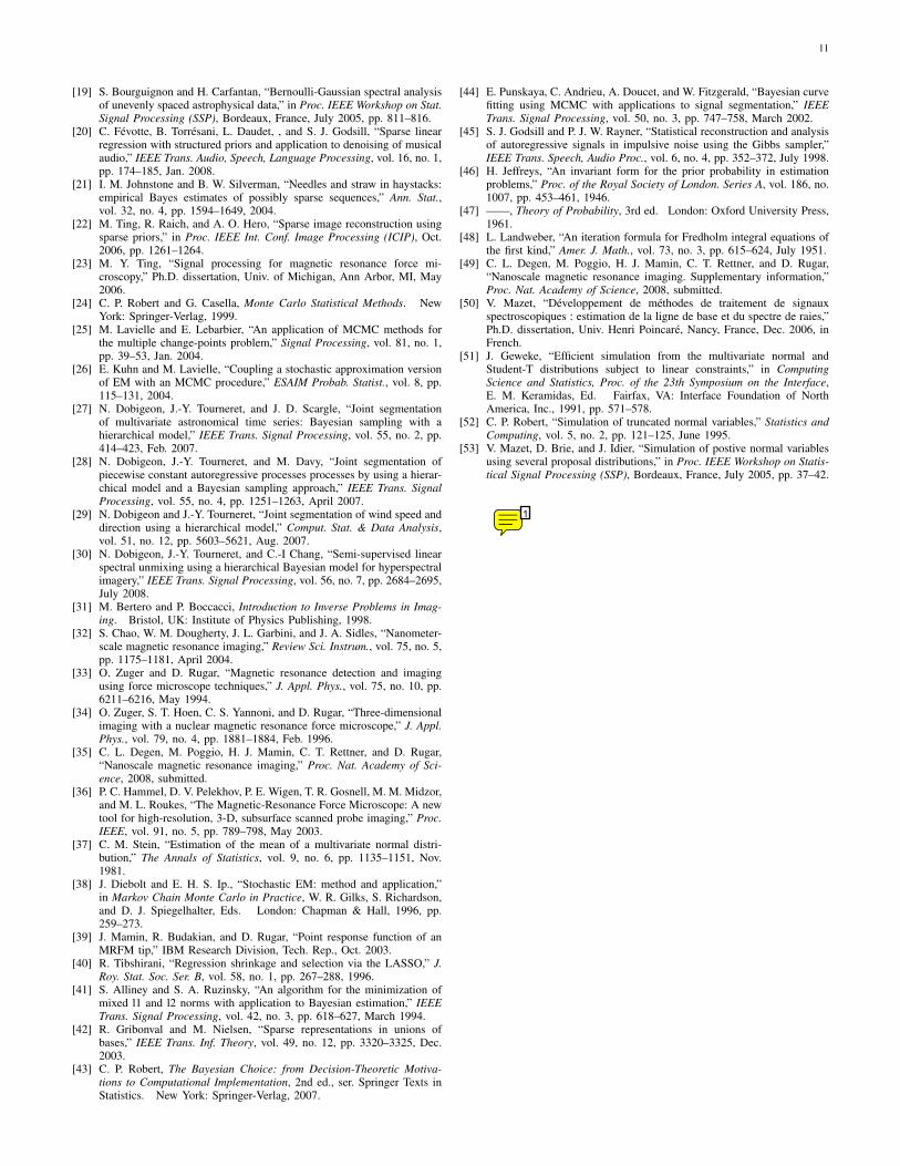
11

[19] S. Bourguignon and H. Carfantan, “Bernoulli-Gaussian spectral analysisof unevenly spaced astrophysical data,” in Proc. IEEE Workshop on Stat.Signal Processing (SSP), Bordeaux, France, July 2005, pp. 811–816.

[20] C. Fevotte, B. Torresani, L. Daudet, , and S. J. Godsill, “Sparse linearregression with structured priors and application to denoising of musicalaudio,” IEEE Trans. Audio, Speech, Language Processing, vol. 16, no. 1,pp. 174–185, Jan. 2008.

[21] I. M. Johnstone and B. W. Silverman, “Needles and straw in haystacks:empirical Bayes estimates of possibly sparse sequences,” Ann. Stat.,vol. 32, no. 4, pp. 1594–1649, 2004.

[22] M. Ting, R. Raich, and A. O. Hero, “Sparse image reconstruction usingsparse priors,” in Proc. IEEE Int. Conf. Image Processing (ICIP), Oct.2006, pp. 1261–1264.

[23] M. Y. Ting, “Signal processing for magnetic resonance force mi-croscopy,” Ph.D. dissertation, Univ. of Michigan, Ann Arbor, MI, May2006.

[24] C. P. Robert and G. Casella, Monte Carlo Statistical Methods. NewYork: Springer-Verlag, 1999.

[25] M. Lavielle and E. Lebarbier, “An application of MCMC methods forthe multiple change-points problem,” Signal Processing, vol. 81, no. 1,pp. 39–53, Jan. 2004.

[26] E. Kuhn and M. Lavielle, “Coupling a stochastic approximation versionof EM with an MCMC procedure,” ESAIM Probab. Statist., vol. 8, pp.115–131, 2004.

[27] N. Dobigeon, J.-Y. Tourneret, and J. D. Scargle, “Joint segmentationof multivariate astronomical time series: Bayesian sampling with ahierarchical model,” IEEE Trans. Signal Processing, vol. 55, no. 2, pp.414–423, Feb. 2007.

[28] N. Dobigeon, J.-Y. Tourneret, and M. Davy, “Joint segmentation ofpiecewise constant autoregressive processes processes by using a hierar-chical model and a Bayesian sampling approach,” IEEE Trans. SignalProcessing, vol. 55, no. 4, pp. 1251–1263, April 2007.

[29] N. Dobigeon and J.-Y. Tourneret, “Joint segmentation of wind speed anddirection using a hierarchical model,” Comput. Stat. & Data Analysis,vol. 51, no. 12, pp. 5603–5621, Aug. 2007.

[30] N. Dobigeon, J.-Y. Tourneret, and C.-I Chang, “Semi-supervised linearspectral unmixing using a hierarchical Bayesian model for hyperspectralimagery,” IEEE Trans. Signal Processing, vol. 56, no. 7, pp. 2684–2695,July 2008.

[31] M. Bertero and P. Boccacci, Introduction to Inverse Problems in Imag-ing. Bristol, UK: Institute of Physics Publishing, 1998.

[32] S. Chao, W. M. Dougherty, J. L. Garbini, and J. A. Sidles, “Nanometer-scale magnetic resonance imaging,” Review Sci. Instrum., vol. 75, no. 5,pp. 1175–1181, April 2004.

[33] O. Zuger and D. Rugar, “Magnetic resonance detection and imagingusing force microscope techniques,” J. Appl. Phys., vol. 75, no. 10, pp.6211–6216, May 1994.

[34] O. Zuger, S. T. Hoen, C. S. Yannoni, and D. Rugar, “Three-dimensionalimaging with a nuclear magnetic resonance force microscope,” J. Appl.Phys., vol. 79, no. 4, pp. 1881–1884, Feb. 1996.

[35] C. L. Degen, M. Poggio, H. J. Mamin, C. T. Rettner, and D. Rugar,“Nanoscale magnetic resonance imaging,” Proc. Nat. Academy of Sci-ence, 2008, submitted.

[36] P. C. Hammel, D. V. Pelekhov, P. E. Wigen, T. R. Gosnell, M. M. Midzor,and M. L. Roukes, “The Magnetic-Resonance Force Microscope: A newtool for high-resolution, 3-D, subsurface scanned probe imaging,” Proc.IEEE, vol. 91, no. 5, pp. 789–798, May 2003.

[37] C. M. Stein, “Estimation of the mean of a multivariate normal distri-bution,” The Annals of Statistics, vol. 9, no. 6, pp. 1135–1151, Nov.1981.

[38] J. Diebolt and E. H. S. Ip., “Stochastic EM: method and application,”in Markov Chain Monte Carlo in Practice, W. R. Gilks, S. Richardson,and D. J. Spiegelhalter, Eds. London: Chapman & Hall, 1996, pp.259–273.

[39] J. Mamin, R. Budakian, and D. Rugar, “Point response function of anMRFM tip,” IBM Research Division, Tech. Rep., Oct. 2003.

[40] R. Tibshirani, “Regression shrinkage and selection via the LASSO,” J.Roy. Stat. Soc. Ser. B, vol. 58, no. 1, pp. 267–288, 1996.

[41] S. Alliney and S. A. Ruzinsky, “An algorithm for the minimization ofmixed l1 and l2 norms with application to Bayesian estimation,” IEEETrans. Signal Processing, vol. 42, no. 3, pp. 618–627, March 1994.

[42] R. Gribonval and M. Nielsen, “Sparse representations in unions ofbases,” IEEE Trans. Inf. Theory, vol. 49, no. 12, pp. 3320–3325, Dec.2003.

[43] C. P. Robert, The Bayesian Choice: from Decision-Theoretic Motiva-tions to Computational Implementation, 2nd ed., ser. Springer Texts inStatistics. New York: Springer-Verlag, 2007.

[44] E. Punskaya, C. Andrieu, A. Doucet, and W. Fitzgerald, “Bayesian curvefitting using MCMC with applications to signal segmentation,” IEEETrans. Signal Processing, vol. 50, no. 3, pp. 747–758, March 2002.

[45] S. J. Godsill and P. J. W. Rayner, “Statistical reconstruction and analysisof autoregressive signals in impulsive noise using the Gibbs sampler,”IEEE Trans. Speech, Audio Proc., vol. 6, no. 4, pp. 352–372, July 1998.

[46] H. Jeffreys, “An invariant form for the prior probability in estimationproblems,” Proc. of the Royal Society of London. Series A, vol. 186, no.1007, pp. 453–461, 1946.

[47] ——, Theory of Probability, 3rd ed. London: Oxford University Press,1961.

[48] L. Landweber, “An iteration formula for Fredholm integral equations ofthe first kind,” Amer. J. Math., vol. 73, no. 3, pp. 615–624, July 1951.

[49] C. L. Degen, M. Poggio, H. J. Mamin, C. T. Rettner, and D. Rugar,“Nanoscale magnetic resonance imaging. Supplementary information,”Proc. Nat. Academy of Science, 2008, submitted.

[50] V. Mazet, “Developpement de methodes de traitement de signauxspectroscopiques : estimation de la ligne de base et du spectre de raies,”Ph.D. dissertation, Univ. Henri Poincare, Nancy, France, Dec. 2006, inFrench.

[51] J. Geweke, “Efficient simulation from the multivariate normal andStudent-T distributions subject to linear constraints,” in ComputingScience and Statistics, Proc. of the 23th Symposium on the Interface,E. M. Keramidas, Ed. Fairfax, VA: Interface Foundation of NorthAmerica, Inc., 1991, pp. 571–578.

[52] C. P. Robert, “Simulation of truncated normal variables,” Statistics andComputing, vol. 5, no. 2, pp. 121–125, June 1995.

[53] V. Mazet, D. Brie, and J. Idier, “Simulation of postive normal variablesusing several proposal distributions,” in Proc. IEEE Workshop on Statis-tical Signal Processing (SSP), Bordeaux, France, July 2005, pp. 37–42.

1

Page: 11

Number: 1 Author: vmuser Subject: Sticky Note Date: 9/17/2008 1:25:38 PM Include other references: M. Ting, R. Raich and A. O. Hero, "Empirical approaches to sparse image reconstruction," submitted to IEEE Trans. on Image Processing, 2008. Kyle Herrity, Raviv Raich and Alfred O. Hero, "Blind deconvolution for sparse molecular imaging," IEEE Intl Conf. on Acoustics, Speech and Signal Processing , April 2008.

Documents

Bayesian sparse image reconstruction. Application to …web.eecs.umich.edu/~hero/Preprints/Summary of Comments on... · 2008-09-18 · Bayesian sparse image reconstruction. Application