Bayesian Robust Principal Component Analysis - All …people.ee.duke.edu/~lcarin/LRS_09.pdf · 1 Bayesian Robust Principal Component Analysis 1;2Xinghao Ding, 1Lihan He and 1Lawrence

1

Bayesian Robust Principal Component Analysis

1,2Xinghao Ding, 1Lihan He and 1Lawrence Carin1Department of Electrical & Computer Engineering

Duke University

Durham, NC 27708-0291, USA2Department of Communication Engineering

Xiamen University

Xiamen, Fujian, 361005, China

Email: [email protected], [email protected], [email protected]

Abstract

A hierarchical Bayesian model is considered for decomposing a matrix into low-rank and sparse

components, assuming the observed matrix is a superposition of the two. The matrix is assumed

noisy, with unknown and possibly non-stationary noise statistics. The Bayesian framework infers an

approximate representation for the noise statistics while simultaneously inferring the low-rank and

sparse-outlier contributions; the model is robust to a broad range of noise levels, without having to change

model hyperparameter settings. In addition, the Bayesian framework allows exploitation of additional

structure in the matrix. For example, in video applications each row (or column) corresponds to a video

frame, and we introduce a Markov dependency between consecutive rows in the matrix (corresponding

to consecutive frames in the video). The properties of this Markov process are also inferred based on the

observed matrix, while simultaneously denoising and recovering the low-rank and sparse components.

We compare the Bayesian model to a state-of-the-art optimization-based implementation of robust PCA;

considering several examples, we demonstrate competitive performance of the proposed model.

Index Terms

Bayesian modeling, principal component analysis, low-rank matrix, sparsity, Markov dependency

I. INTRODUCTION

Natural high-dimensional data, such as images, video, documents, biological data, and social-

network data often reside in a low-dimensional subspace [1] or low-dimensional manifold [2], [3].

April 14, 2011 DRAFT

2

For example, the frames in a video sequence typically reside in a subspace of dimension much

smaller than that of the number of frame pixels, due to strong correlation between consecutive

video frames. Movie rating data constitute another example, among which the Netflix Prize

[4] is perhaps the most famous example. The rating matrix is typically low-rank, because of

similarities among movies and among users/people.

Principal component analysis (PCA) [5], [6], computed via a singular value decomposition

(SVD), is a common tool for extracting low-dimensional information from the aforementioned

high-dimensional data. Utilizing SVD, a data matrix L ∈ RN×M with rank r can be decomposed

as

L = DΛW T =r∑

i=1

λidiwTi (1)

where diagonal matrix Λ = diag(λ1, ..., λr) ∈ Rr×r consists of singular values of L, D =

[d1, ...,dr] ∈ RN×r and W = [w1, ...,wr] ∈ RM×r are the matrices of left- and right-singular

vectors, respectively. If L is low-rank, r ≪ min(N,M).

Low-rank matrix representations have recently received significant attention. In these studies

two types of noise models are often considered. One class corresponds to generally small-

magnitude perturbations to all matrix elements [7], [8] (e.g., i.i.d. Gaussian noise added to each

matrix element). If the noise energy is small relative to the dominant singular values of the

SVD, this noise class often manifests relatively modest changes to a noise-free PCA analysis.

Specifically, it often yields small perturbations to the singular values, but does not significantly

impact the principal vectors, and shrinkage methods may be employed for denoising [9]. The

second noise class is sparse and of arbitrary amplitude, it impacting a small subset of the matrix

elements [10], [11]. For example, a moving object in video, in the presence of a static background,

manifests such sparse noise (if the matrix has rows/columns defined by the video frames). In

this situation the sparse outliers may easily corrupt classical PCA, causing the singular vectors

and singular values to change dramatically.

Many algorithms have been proposed to address the brittleness of classical PCA with respect

to outlier (sparse) noise, yielding the field of robust PCA [12], [13], [14], [15], [16]. However,

these previous methods are typically computationally inefficient, and they do not possess the

strong performance guarantees provided by very recent work [10], [17]. In particular, in [10],

[17], [11] the authors have proposed convex optimization to address the robust PCA problem.


3

The observation matrix is assumed represented as Y = L + S, where L is a low-rank matrix

and S is a sparse matrix with a small fraction of (arbitrary magnitude) nonzero entries. This

research seeks to solve for L with the following optimization problem:

minL,S∥L∥∗ + ζ∥S∥1 s.t. L+ S = Y (2)

where ∥ · ∥∗ and ∥ · ∥1 denote the matrix nuclear norm (sum of singular values) and ℓ1 norm,

respectively, and ζ > 0 is a parameter to balance the two terms. Candes et al. showed in [17]

that under broad conditions the proposed convex optimization method exactly recovers L and

S, and the results in [10], [17] demonstrated encouraging performance on real data.

In practice, measurement noise (of the first type discussed above) exists everywhere within

the matrix and sometimes this dense (distributed) noise contribution cannot be ignored. The

problem of additive noise of this type, denoted E, is discussed in [10], [17], with this addressed

explicitly in [18]. The work in [18] modified (2) to include an error term, i.e., minL,S ∥L∥∗ +

ζ∥S∥1 + (2µ)−1∥Y − L− S∥2F , with ∥ · ∥F denoting the Frobenius norm. However, to choose

the balance parameter µ, the noise variance has to be known.

In this paper we also consider the observation matrix Y = L+ S +E, with the presence of

both sparse noise S and the dense noise E. Although E is usually not desired and is discarded,

the sparse outliers S are sometimes of interest (e.g., for tracking moving entities in video).

Therefore, in the remainder of the paper we do not regard the sparse outliers as noise; we

call L, S and E the low-rank, sparse, and noise components, respectively. In the proposed

Bayesian framework, the noise statistics of E are learned (approximately) based on the data,

simultaneous with the learning of L and S. When presenting results, we demonstrate that the

proposed Bayesian model is robust to a broad range of noise variance (and to nonstationary

noise), without having to change model hyperparameters.

The Bayesian model infers approximations to full posterior distributions on all model pa-

rameters, and therefore we obtain approximate probability distributions for L, S and E. One

may compute the mean values from the posterior distributions, if a point (single) estimate is

desired; however, the estimate to the full posterior may be used to place “error bars” on the

inferred mean matrices S and L, of interest when making subsequent classification/tracking

inferences, for example. An advantage of the Bayesian model is that prior knowledge can be

flexibly incorporated, with minor changes to the model structure and computations. For example,


4

the flexibility of the Bayesian framework allows us to exploit anticipated structure in the sparse

component. As an example, consider video analysis, with the video frames defining the matrix

columns. Assume we attempt to extract temporally and spatially localized moving objects (sparse

component) from the static (or near-static) background (low-rank component), in the presence of

frame-dependent additive noise E. It is desirable to account for the correlation in the properties of

the sparse part of the video, from frame to frame (column to column in the matrix). In this paper,

we assume a Markov dependency in time and space for the sparse component, which implies

a Markov property between the sparse components of consecutive matrix columns. Within a

Bayesian framework, this structure is readily imposed, with the Markov properties inferred via

the observed matrix (i.e., the form of the Markov model is imposed, with the data used to infer

the Markov parameters).

In related statistical analysis of matrices, a probabilistic interpretation of PCA has been

introduced, termed probabilistic PCA [19]. Based on this framework, Bayesian models for robust

PCA have been proposed [20], [21]. Rather than considering the sparse outliers in S as discussed

above, the work in [20], [21] considers outliers existing in the dense noise E. Therefore these

models assume Y = L+E, with the noise term E modeled by heavy-tailed distributions, such as

Laplacian distribution [20] or the Student-t distribution [21]. Although these types of distributions

may describe outliers in dense noise, the models do not have the ability to distinguish sparse

outliers from small dense noise, especially if the sparse outliers are of particular interest.

The work presented here is also closely related to low-rank matrix completion (for matrices

with missing entries). There has been significant recent interest in this problem, addressed based

on convex optimization [22], [23] or based on a hierarchical Bayesian framework [24], [25]. The

objective of the problem is to approximate a matrix (with noisy entries) by a low-rank matrix

and to predict the missing entries. In a Bayesian framework, the low-rank matrix L ∈ RN×M

can be decomposed into two matrices, i.e., L = UV , with U ∈ RN×r and V ∈ Rr×M , where

r is the rank of L. Note that this matrix factorization form is the SVD decomposition of L in

(1) if the singular-value matrix Λ is absorbed by D and/or W . Because of the flexibility of

the Bayesian framework, many variants of this matrix factorization form have been proposed

to improve the model robustness and performance [26], [27]. Although we do not consider this

here, if the matrix under test Y = L+S+E is missing entries at random, the proposed model

can consider this as well, and can make estimates for the missing entries (in terms of the low-


5

rank term L). The S term may be viewed as defining a sparse set of matrix entries that should

be removed when estimating L; in the matrix completion problem the location of these entries

– the missing entries – are of course known, while in the robust PCA problem the location of

S must be inferred, while also estimating values of L, S and E.

This paper is also related to recent developments in Bayesian compressive sensing [28], [29],

[30], which aims to achieve sparse signal reconstruction. Typically, in a Bayesian framework, the

sparseness-promoting prior (e.g., a hierarchical normal-gamma prior in [28]) is imposed on the

signal of interest, and the posterior distribution of the sparse signal is inferred. Known statistical

structure within the sparse coefficients can be readily embedded in the model. For example, the

work in [31], [32] has explicitly imposed a hidden Markov tree structure within the wavelet

decomposition of an image. The manner in which we track S from frame to frame in video is

related to the tree structure used in [31].

The remainder of the paper is organized as follows. In Section II we present the proposed

Bayesian low-rank and sparse model, and relate it to the optimization-based approaches in the

literature. In Section III the Markov dependency for the sparse component is introduced, of

particular interest in video applications. Section IV provides the computational inference methods

considered for the model, with experimental results presented in Section V. We conclude in

Section VI.

II. BAYESIAN LOW-RANK AND SPARSE MODEL

We assume that the observed data matrix Y ∈ RN×M is the superposition of three parts:

low-rank component L ∈ RN×M , sparse component S ∈ RN×M , and noise term E ∈ RN×M .

The sparse component S may have large magnitude (relative to the magnitude of L) but sparse

support (only a small fraction of entries in S are nonzero), and E has generally small magnitude

but dense support. Given observation Y = L+ S +E, our objective is to recover L and S.

The proposed Bayesian model is

Y = D(ZΛ)W +B ◦X +E (3)

where D ∈ RN×K ,W ∈ RK×M , Λ ∈ RK×K is a diagonal matrix, X ∈ RN×M , and ◦ denotes

the Hadamard (pointwise) product. The diagonal matrix Z has binary entries along the diagonal,

and the binary matrix B ∈ {0, 1}N×M is sparse. The integer K defines the largest possible rank

that may be inferred for L, and K is set to a large value. Below we explain the model in detail.


6

A. Low-rank component

The low-rank component is modeled as L = D(ZΛ)W . Note that this is similar to the SVD

decomposition in (1), but here we introduce an extra diagonal matrix Z, with diagonal elements

zkk ∈ {0, 1} for k = 1, ..., K. The product of the two matrices, ZΛ, is still a diagonal matrix

and plays a role analogous to the singular values of L. The introduction of Z decouples the

rank learning and the singular-value learning, in that the magnitudes of the singular values are

inferred in Λ and the rank is learned as r = ∥Z∥0. Since the rank of L is unknown, we choose

large K, and hence we expect that the diagonal entries of ZΛ are sparse (if they are not, we

know the selected K was not large enough).

The binary diagonal matrix Z is modeled as

zkk ∼ Bernoulli(pk), pk ∼ Beta(α0, β0), k = 1, ...K (4)

with hyperparameters α0 > 0 and β0 > 0. The sparseness of the diagonal of Z is explicitly

imposed through hyperparameters α0 and β0. Note that E[pk] = α0/(α0+β0), where E[·] denotes

the expectation of a random variable. To impose the sparseness on the diagonal of Z, we may

let α0/(α0 + β0) ≪ 1, and therefore it is probable that pk is close to zero. In our experiments

we specify α0 = 1/K and β0 = (K − 1)/K.

Each diagonal entry in Λ, denoted as λkk for k = 1, ..., K, is drawn from a normal-gamma

distribution:

λkk ∼ N (0, τ−1), k = 1, ..., K, τ ∼ Gamma(a0, b0), (5)

with hyperparameters a0 > 0 and b0 > 0. In (5) the we set a0 = b0 = 10−6 [33].

The columns of matrices D = [d1, ...,dK ] and W = [w1, ...,wM ] are assumed to be drawn

from normal distributions:

dk ∼ N (0,1

NIN), k = 1, ..., K (6)

wm ∼ N (0,1

KIK), m = 1, ...,M (7)

where IN denotes an N × N identity matrix. Note that when N and K are large the columns

of D are approximately orthogonal to each other (also true for the columns of W ), consistent

with their role in an SVD decomposition; however, here we only impose that the columns of D

span the space of the principal vectors, without explicitly requiring orthonormality. One could


7

explicitly impose orthonormality if desired [34], but this comes at significant computational cost

and it has been found unnecessary in our experiments.

The decomposition of the low-rank component L = D(ZΛ)W can also be viewed from the

standpoint of factor analysis. We may rewrite each column of L = [l1, ..., lM ] as

lm = D(ZΛ)wm =K∑k=1

zkkλkkwkmdk, m = 1, ...,M. (8)

This suggests that each column of L can be viewed as a weighted sum of the dictionary elements

(columns) in D, and the K can be seen as the size of the dictionary. The weights {zkkλkk}k=1:K

globally determine all the dictionary elements that are active to construct L, and the weights

{wkm}k=1:K determine the importance of the selected dictionary elements for representation of

the mth column of L. Equation (8) is also useful in the model inference, and will be revisited

in Section IV.

B. Sparse Component

The sparse component is modeled as S = B ◦X , where B is a binary matrix. Again, this

approach separates the learning of sparseness from the learning of values, such that the zero

component in S is exactly zero. Each column of the binary matrix B = [b1, ..., bM ] is modeled

as

bm ∼N∏

n=1

Bernoulli(πn), m = 1, ...,M, πn ∼ Beta(α1, β1), n = 1, ...N. (9)

Here the nth row in B shares a common prior parameter πn. In addition, the model is robust to

noise because updating πn uses all data in the nth row of B. As an alternative approach, each

entry in B may have its own prior parameter. This alternative is convenient for introducing further

structure into the prior for the sparse component, such as a Markov property, as demonstrated

in Section III. A sparseness prior is explicitly placed on B, by specifying α1 and β1 such that

α1/(α1+β1)≪ 1, as explained in (4). In our experiments we let α1 = 1/N and β1 = (N−1)/N .

The columns of X = [x1, ...,xM ] are assumed drawn from a normal-gamma distribution:

xm ∼ N (0, ν−1IN), m = 1, ...,M, ν ∼ Gamma(c0, d0). (10)

We let all the data in X share the same precision parameter ν, to reduce model complexity and

increase robustness. As in (5), typically we set c0 = d0 = 10−6.


8

C. Noise Component

We assume the measurement noise is drawn i.i.d. from a Gaussian distribution, and the

noise affects all the measurements. Note that this construction is only within the prior, and

the approximation to the posterior of E can infer perturbations to this prior, if present, moving

beyond the i.i.d. Gaussian model, if the data so indicates. The noise variance or precision is

assumed unknown, and is learned within the model inference. Mathematically, the noise is

modeled as

enmiid∼ N (0, γ−1), n = 1, ..., N, m = 1, ...,M, γ ∼ Gamma(e0, f0) (11)

where enm denotes the entry at row n and column m of E. As in (5) and (10), we set hyperpa-

rameters e0 = f0 = 10−6. One should note that while there appear to be many hyperparameters

in the model, as indicated above they are all set in a “standard” manner [33], with no tuning

performed or cross-validation required.

If desired, the model can learn different noise variances for different parts of E. For example,

in a video application, each column/row of Y corresponds to a video frame, and each frame

may in general have its own noise level (we will consider this in the experiments). Let the data

be organized such that each frame represents one column of Y . We may then modify the noise

structure in (11) as

enm ∼ N (0, γ−1m ), n = 1, ..., N, γm ∼ Gamma(e0, f0) (12)

for m = 1, ...,M .

D. Relation to optimization-based approach

We now make connections of the Bayesian model proposed here to optimization-based ap-

proaches [10], [17], [18]. Note that for the low-rank component, we place a sparseness prior on

the singular values, to impose a desire for a small number of non-zero singular values; in [17]

the ℓ0 norm (number of non-zero elements) of the singular values is minimized in the original

objective function, with this relaxed to an ℓ1 norm when solving the problem computationally.

Similarly, for the sparse component, we place a sparseness prior to impose the belief that few

components of S are nonzero, while in [17] the ℓ0 norm of the sparse component is introduced,

with this again relaxed to an ℓ1 norm when performing computations.


9

To see the connection more clearly, note that the negative logarithm of the full posterior

density function of our Bayesian model is

− log p(Θ|Y ,H) =τ

2∥Λ∥2F − log[fBB(Z;H)] + N

2

K∑k=1

∥dk∥22 +1

2

M∑m=1

∥wm∥22

+ν

2∥X∥2F − log[fBB(B;H)] + γ

2∥Y −L− S∥2F

− log[Gamma(τ |H)Gamma(ν|H)Gamma(γ|H)] + Const. (13)

where Θ represents all model parameters, fBB(·|H) represents the beta-Bernoulli prior in (4)

or (9), and H = {α0, β0, α1, β1, a0, b0, c0, d0, e0, f0} are model hyperparameters. Therefore, the

error term (2µ)−1∥Y − L− S∥2F in [18] (where the dense noise is considered) corresponds to

the Gaussian prior placed on the measurement noise in (11). In [18] the authors suggest that

the optimal balance parameter µ is a function of noise variance, which is consistent with the

weight γ2

here. However, in our Bayesian model, we are not required to know the noise variance

a priori, and the model will learn the variance when performing inference. For the low-rank

component, rather than employing an ℓ1 constraint to impose the sparseness of singular values,

we employ a Gaussian prior to obtain a constraint on Frobenius matrix norm ∥Λ∥2F , together with

a beta-Bernoulli distribution to explicitly encourage the sparseness of singular values (like an ℓ0

prior). Similarly for the sparse component, instead of the ℓ1 constraint used in [10], [17], [18], the

constraint on Frobenius matrix norm ∥X∥2F and the beta-Bernoulli distribution are employed to

impose the sparseness (again like an ℓ0 prior). An ℓ1 constraint may also be imposed in a Bayesian

framework, by employing a Laplacian prior (implemented as in Bayesian Lasso [35]). However,

the beta-Bernoulli prior employed here imposes exactly zero entries, while the ℓ1 Laplacian prior

gives many small entries (but not exactly zero). Note also that the ℓ2 regularization in (13) for

dk and wm has been used in previous related optimization approaches [36], and comes naturally

as a consequence of the Gaussian priors on dk and wm.

The differences notwithstanding, we note that there are strong connections between the Bayesian

formulation and the optimization approaches in [10], [17], [18], [36]. Apart from the details in the

differences in the form of − log p(Θ|Y ,H) relative to related optimization-based approaches, the

main difference is that here we use numerical methods to estimate a distribution for the unknown

parameters, while in optimization-based approaches one effectively seeks a single solution that

minimizes a functional analogous to − log p(Θ|Y ,H) (ideally with convexity guarantees [10],


10

[17], [18], [36]).

III. MARKOV DEPENDENCY OF SPARSE TERM IN TIME AND SPACE

In the prior, given parameters π = {πn}n=1:N , the entries in the sparse component S are

assumed to be drawn independently. This is clearly not true for some applications. For example,

in fixed-camera video-surveillance analysis, the (nearly) static background manifests the low-rank

component, and the moving objects are the sparse component. It is clear that the moving objects

are strongly correlated across consecutive frames, and therefore the independence assumption is

inappropriate.

We assume the appearance of the sparse component across frames (time) satisfies a Markov

property. Specifically, if there is a moving object at some place in a frame, it is very likely that

this object will appear at about the same place in the next frame. Let the sparse component of

frame t (t indexes time) be Ft, with the pixel at coordinates (i, j) denoted Ft(i, j). The parent

node of Ft(i, j) is defined as Ft−1(i, j), i.e., the sparse component at the same coordinates in

the previous frame. We may then exploit the belief that if a parent node is non-zero, with a high

probability its child node is also non-zero.

The simple Markov structure imposed above reflects the anticipated dependence imposed by

a moving object across frames. However it is very sensitive to noise. If a noise entry exists in

Ft, it will, with high probability, affect all the later frames. To make the Markov dependency

more robust to noise, we introduce a spatial dependence. We define the neighbor of Ft(i, j) as

N[Ft(i, j)] = {Ft(i′, j′) : |i′ − i| ≤ Ra, |j′ − j| ≤ Ra}, and in our experiments we set Ra = 1.

Other definitions for a spatial neighborhood may also be imposed. We then define the state of

Ft(i, j), denoted as S[Ft(i, j)]:

S[Ft(i, j)] =

active, if ∥N[Ft(i, j)]∥0 ≥ ρ

inactive, otherwise(14)

where ρ is a predefined scalar; we set ρ = 5 in our experiments. This definition imposes that

we consider a node to be in an active state if the sparse component contains at least ρ nonzero

members in its neighborhood. The Markov dependency between a parent and its child is now

modified as: if a parent node is active, then with a high probability its child node is also active.

In this way the sparsity of a child node depends not only on its parent node (in time) but also

on the neighbors of its parent node (in space).


11

With the temporal and spatial assumptions discussed above, we modify the basic model to

impose the dependency on the sparse component S. Assume the tth column of Y is constructed

by concatenating all components of frame t, for 1 ≤ t ≤ M . The Markov dependency is then

imposed by modifying (9) as

bt ∼N∏

n=1

Bernoulli(πnt), t = 1, ...,M,

πnt ∼

Beta(αH , βH) if S[bn,t−1] = active,

Beta(αL, βL) if S[bn,t−1] = inactive,n = 1, ...N, t = 2, ...,M. (15)

For t = 1, we may still use (9) since there are no parent nodes for the first frame. The subscripts

H and L in the model above recall the “high” and “low” states in the Markov tree model used for

wavelet coefficients in compressive sensing [31]. To determine S[bn,t−1], the coordinates (i, j)

can be calculated from n. We let αH/(αH + βH) ≈ 1 and αL/(αL + βL) ≈ 0, so that the

sparseness pattern propagates along time with high probability. Note that a component of S is

not directly non-zero depending on whether it is active/inactive; rather, if a component is in an

active state it has a high probability of being non-zero, while if it is in an inactive state it has

a low probability of being non-zero.

IV. POSTERIOR INFERENCE

In the proposed hierarchical model, the density function at one layer is conjugate to the density

function at the layer above it. This greatly eases the ability to perform computations. Specifically,

we perform computations for an approximation to the posterior density function in two ways:

via Markov chain Monte Carlo (MCMC) analysis [37] implemented using a Gibbs sampler, and

via the variational Bayesian (VB) approximation [38]. In MCMC the posterior distribution is

approximated by a set of samples, collected by iteratively drawing each random variable (model

parameters) from its conditional posterior distribution given the most recent values of all the

other parameters. The MCMC-based Bayesian inference for the model (3)-(11) is summarized in

Algorithm 1, where ym represents the mth column in Y and (a|−) represents random variable

a given all the other random variables in the model. The algorithm starts from a set of initial

values Θ0, and after a large number of burn-in iterations Nburn-in, we consider the Markov chain

has become stable. A number Ncollect of samples {Θ(i)}i=1:Ncollect are then collected to represent

the joint posterior distribution of these random variables.


12

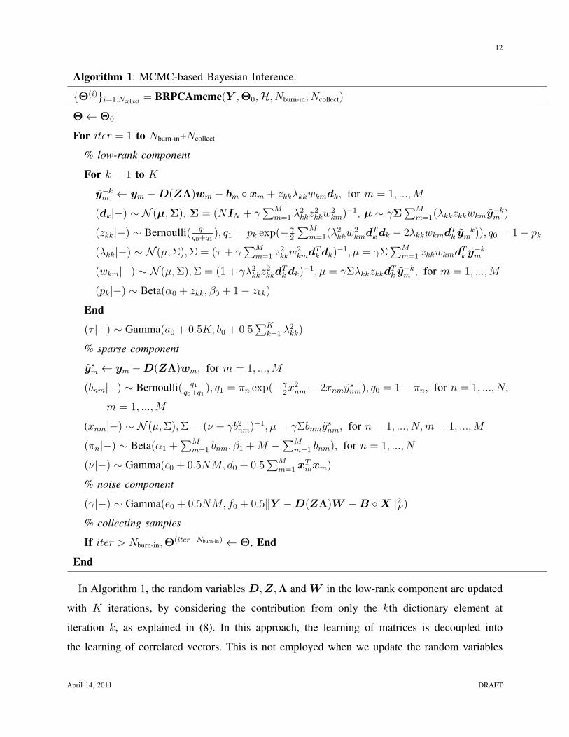
Algorithm 1: MCMC-based Bayesian Inference.

{Θ(i)}i=1:Ncollect = BRPCAmcmc(Y ,Θ0,H, Nburn-in, Ncollect)

Θ← Θ0

For iter = 1 to Nburn-in+Ncollect

% low-rank component

For k = 1 to K

y−km ← ym −D(ZΛ)wm − bm ◦ xm + zkkλkkwkmdk, for m = 1, ...,M

(dk|−) ∼ N (µ,Σ), Σ = (NIN + γ∑M

m=1 λ2kkz

2kkw

2km)

−1, µ ∼ γΣ∑M

m=1(λkkzkkwkmy−km )

(zkk|−) ∼ Bernoulli( q1q0+q1

), q1 = pk exp(−γ2

∑Mm=1(λ

2kkw

2kmd

Tk dk − 2λkkwkmd

Tk y

−km )), q0 = 1− pk

(λkk|−) ∼ N (µ,Σ),Σ = (τ + γ∑M

m=1 z2kkw

2kmd

Tk dk)

−1, µ = γΣ∑M

m=1 zkkwkmdTk y

−km

(wkm|−) ∼ N (µ,Σ),Σ = (1 + γλ2kkz

2kkd

Tk dk)

−1, µ = γΣλkkzkkdTk y

−km , for m = 1, ...,M

(pk|−) ∼ Beta(α0 + zkk, β0 + 1− zkk)

End

(τ |−) ∼ Gamma(a0 + 0.5K, b0 + 0.5∑K

k=1 λ2kk)

% sparse component

ysm ← ym −D(ZΛ)wm, for m = 1, ...,M

(bnm|−) ∼ Bernoulli( q1q0+q1

), q1 = πn exp(−γ2x2nm − 2xnmy

snm), q0 = 1− πn, for n = 1, ..., N,

m = 1, ...,M

(xnm|−) ∼ N (µ,Σ),Σ = (ν + γb2nm)−1, µ = γΣbnmy

snm, for n = 1, ..., N,m = 1, ...,M

(πn|−) ∼ Beta(α1 +∑M

m=1 bnm, β1 +M −∑M

m=1 bnm), for n = 1, ..., N

(ν|−) ∼ Gamma(c0 + 0.5NM, d0 + 0.5∑M

m=1 xTmxm)

% noise component

(γ|−) ∼ Gamma(e0 + 0.5NM, f0 + 0.5∥Y −D(ZΛ)W −B ◦X∥2F )

% collecting samples

If iter > Nburn-in,Θ(iter−Nburn-in) ← Θ, End

End

In Algorithm 1, the random variables D,Z,Λ and W in the low-rank component are updated

with K iterations, by considering the contribution from only the kth dictionary element at

iteration k, as explained in (8). In this approach, the learning of matrices is decoupled into

the learning of correlated vectors. This is not employed when we update the random variables


13

of the sparse component, because the entries in the sparse component are assumed independent.

Furthermore, we factorize p(wm) in the inference, p(wm) =∏K

k=1 p(wkm), to avoid the inversion

of a large matrix, reducing the computational burden. Note that with the MCMC inference, this

factorization of p(wm) does not mean that the entries of W are independent, since each random

variable is drawn from a distribution conditioned on all other random variables.

For the model with Markov dependency imposed on the sparse component, Algorithm 1 is

only slightly modified when sampling bnm and πnm, for n = 1, ..., N,m = 1, ...,M . Specifically,

we have:

(bnm|−) ∼ Bernoulli(q1

q0 + q1), q1 = πnm exp(−γ

2x2nm − 2xnmy

snm), q0 = 1− πnm, (16)

(πnm|−) ∼

Beta(α1 + bnm, β1 + 1− bnm) if m = 1

Beta(αH + bnm, βH + 1− bnm) if m > 1,S[bn,m−1] = active,

Beta(αL + bnm, βL + 1− bnm) if m > 1,S[bn,m−1] = inactive.

(17)

The variational Bayesian (VB) inference employs a set of distributions q(Θ) to approximate

the true posterior distributions p(Θ|Y ), and uses a lower bound F to approximate the true log-

likelihood of the model log p(Y |Θ). The algorithm iteratively updates q(Θ) so that F approaches

to log p(Y |Θ) until convergence. Here we omit the update equations for simplicity. Readers may

refer to [38] for details on VB inference.

For the proposed model the computational complexity of a single MCMC and VB iteration

is approximately the same. However, the MCMC method requires a large number of burn-in

iterations, followed by a sufficient number of iterations to collect Θ samples. By contrast, the

VB method directly updates the hyperparameters of q(Θ), and therefore the latest update of q(Θ)

represents the distribution of Θ. After tens of iterations the VB algorithm usually converges,

with convergence inferred by monitoring the quantitative criterion – lower bound F . However,

as mentioned above, the VB solution may find a local-optimal solution (it is not guaranteed

to converge to a globally-optimal best solution). We have found Gibbs sampling to work quite

effectively in practice for this problem, with the mean of the desired parameters converging

relatively quickly (even when the number of samples is too small to accurately represent the full

posterior density function). Therefore, all results presented below will be for the Gibbs sampler,

with discussions also provided that summarize our experience with the VB analysis.


14

V. EXPERIMENTAL RESULTS

A. Simulation

Reconstruction accuracy. We first demonstrate the performance of the proposed algorithm

on simulated data. The data are generated similar to that in [17]. We consider square matrices of

varying dimension N = 500, 1000, 1500. The low-rank component L ∈ RN×N is generated as a

product of two independent N × r matrices whose elements are drawn i.i.d. from N (0, 1/N).

The sparse component S ∈ RN×N is generated such that the non-zero elements are located

uniformly at random and the amplitudes are drawn uniformly at random in the range [-1, 1].

The observation Y = L+S +E, with elements of E drawn i.i.d. from N (0, σ2). We consider

two situations: a noise free case with σ = 0 and a noisy case with σ = 10−4.

The proposed model (3)-(11) is applied to infer the distributions of the low-rank and sparse

components, with estimates denoted L and S, respectively. We set the largest possible rank as

K = 200, and the model hyperparameters are specified as follows: a0 = b0 = c0 = d0 = e0 =

f0 = 10−6, α0 = 1/K, β0 = (K−1)/K, α1 = 0.1N and β1 = 0.9N . The reconstruction accuracy

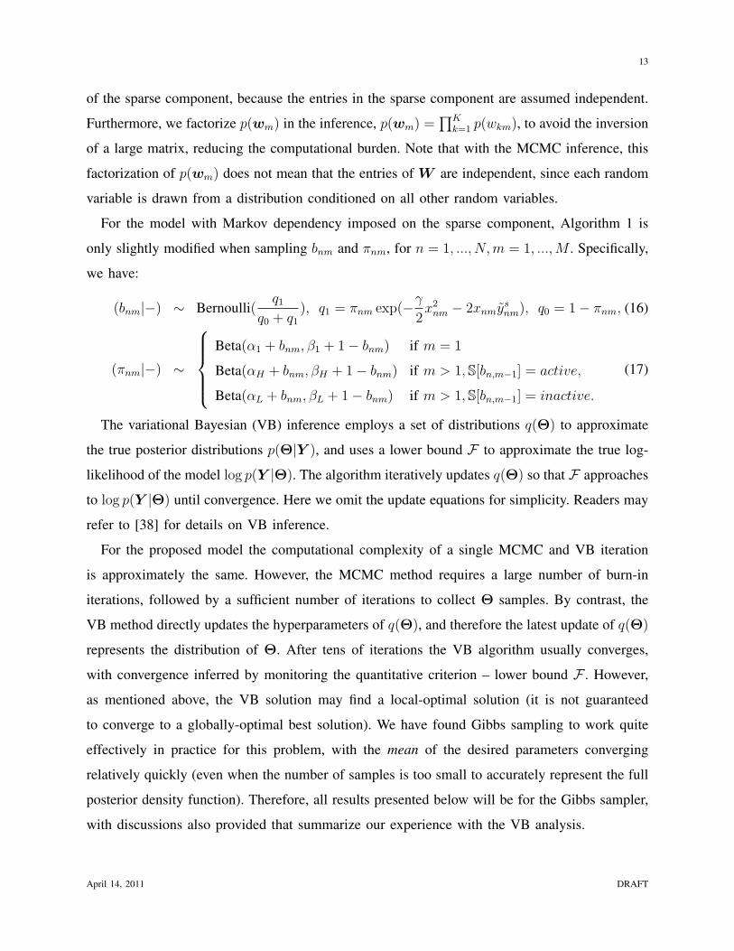
are shown in Tables I(a) and II(a), for the noise free case and the noisy case, respectively. All

results are based on MCMC inference with 25000 burn-in iterations followed by 5000 collection

samples. In Tables I(a) and II(a), we show results for the mean values of estimated L and S,

but we have access to “error bars”, which will be demonstrated later in a real video example.

In Tables I and II three metrics are used to evaluate the reconstruction accuracy of the

algorithm: rank(L), ∥S∥0 and ∥L−L∥F∥L∥F

. A good reconstruction should have accurate estimate

of rank(L) and ∥S∥0, and at the same time have small reconstruction errors for the low-rank

component, evaluated as ∥L−L∥F∥L∥F

. The reconstruction error for the sparse component, ∥S−S∥F∥S∥F

, is

usually small as long as the number of nonzero elements in the sparse component is estimated

accurately; therefore it is not considered here. From Tables I(a) and II(a) we observe that the

proposed algorithm is able to successfully estimate L and S with either noise-free or noisy

observation, even with 10% of the elements in the sparse components nonzero.

As a comparison, in Tables I(b) and II(b)-(c) we show results on the same data set from a

state-of-the-art algorithm: optimization-based robust PCA algorithm proposed in [10]1. Recall

1We used the MATLAB codes of exact_alm_rpca package [39], downloaded from

http://watt.csl.illinois.edu/ perceive/matrix-rank/home.html .


15

(a) Bayesian robust PCA

N rank(L) ∥S∥0 rank(L) ∥L−L∥F∥L∥F

∥S∥0500 25 12500 25 1.1× 10−4 12499

1000 50 50000 50 9.5× 10−5 49998

1500 75 112500 75 1.2× 10−4 112492

500 25 25000 25 1.2× 10−4 24999

1000 50 100000 50 9.9× 10−5 99996

1500 75 225000 75 1.1× 10−4 224985

(b) Optimization-based robust PCA, Tol = 10−6


∥S∥0500 25 12500 25 3.6× 10−6 12505

1000 50 50000 50 2.0× 10−6 50000

1500 75 112500 75 3.8× 10−6 112496

500 25 25000 25 3.5× 10−6 25002

1000 50 100000 50 4.3× 10−6 100013

1500 75 225000 75 5.4× 10−6 225008

TABLE I

COMPARISON OF RECONSTRUCTION ACCURACY FOR NOISE-FREE OBSERVATION (σ = 0). THE TRUE RANK OF THE MATRIX

L IS SET AS 5%N , AND THE NUMBER OF NONZERO SPARSE ELEMENTS IS 5%N2 AND 10%N2 FOR THE TOP AND THE

BOTTOM OF EACH TABLE, RESPECTIVELY.

that in [10] the model is assumed Y = L + S and there is no noise term. However, the

algorithm requires a pre-specified tolerance Tol as a stop criterion. When ∥Y −L−S∥F∥Y ∥F

< Tol,

the algorithm stops. This tolerance is clearly related to the noise level the model assumes when

solving for L and S. In the noise-free situation, we set a small tolerance Tol = 10−6, and the

reconstruction is very accurate (see Table I(b)). However, we observe that in a noisy situation,

the optimization-based algorithm is very sensitive to this tolerance setting. In Table II(b), when

Tol = 7.3× 10−4, the model gives a good reconstruction, but if we change the tolerance from

7.3 × 10−4 to 7.2 × 10−4, the estimation of the rank and the number of sparse elements fails

badly (see Table II(c)). By contrast, the proposed Bayesian model is robust to the noise, with no

tuning or optimization required for the model hyperparameters (the same hyperparameters are

used for all examples, both noisy and noise-free, toy and real).

It should be pointed out that on this toy data set the computation time for the proposed

model is much longer than that from the optimization-based algorithm. This is because the


16



∥S∥0500 25 12500 25 4.5× 10−3 12495

1000 50 50000 50 6.4× 10−3 49990

1500 75 112500 75 7.9× 10−3 112500

500 25 25000 25 4.7× 10−3 24994

1000 50 100000 50 6.6× 10−3 100002

1500 75 225000 75 8.1× 10−3 225011

(b) Optimization-based robust PCA, Tol = 7.3× 10−4


∥S∥0500 25 12500 25 3.4× 10−3 12501

1000 50 50000 50 5.1× 10−3 49951

1500 75 112500 75 6.5× 10−3 112380

(c) Optimization-based robust PCA, Tol = 7.2× 10−4


∥S∥0500 25 12500 58 3.4× 10−2 42474

1000 50 50000 119 4.9× 10−3 169985

1500 75 112500 172 5.9× 10−3 377216

TABLE II

RECONSTRUCTION ACCURACY FOR NOISY OBSERVATION, WITH NOISE STANDARD DEVIATION σ = 10−4 . FOR SIMPLICITY

THE RESULTS FOR ∥S∥0 = 10%N2 ARE NOT SHOWN IN (B) AND (C).

computational complexity of the model is O(K(N + M) + MN), and if K is large this is

expensive (we specified K = 200). In addition, the MCMC convergence speed is closely related

to the true rank of L. A large rank results in a slow convergence. However, in a real application,

for example, video surveillance, usually the rank of L is very low. We may therefore select a

relatively small K, and the MCMC convergence is fast. In this situation the computational time

is comparable to that from the optimization-based algorithm; this is demonstrated below.

Robustness to noise. To further examine the robustness of the proposed model to noisy

observations, we fix N = 100, rank(L) = 5, ∥S∥0 = 500, let the elements of two independent

N×r matrices whose product generates L are drawn i.i.d. from N (0, 1), and let the magnitudes

of the non-zero elements in S are drawn uniformly in the range [−500, 500]. We let the noise

standard deviation change from σ = 0 to σ = 1 with step size 0.01. Figure 1 plots the

reconstruction quality as a function of noise level, solved with the proposed model and using


17

the optimization-based model in [10]. For the optimization-based algorithm, since the results are

sensitive to the tolerance, we set three different values for the tolerance: Tol = 0.001, 0.01 and

0.03.

In Figure 1 the reconstruction quality is represented by rank(L), ∥S∥0 and ∥L−L∥F∥L∥F

. For the

proposed model, we also plot the inferred noise standard deviation σ (mean value). It is observed

from Figure 1(a) that the Bayesian model may adaptively estimate the noise variance, and gives

good reconstruction results. We notice that the Bayesian rank estimate is not perfect occasionally.

By examining the result, we find that when the inferred rank(L) = 6, the sixth singular value

is very small. Therefore, it has minimal impact to the reconstruction quality, which can be

verified from ∥S∥0 and ∥L−L∥F∥L∥F

. As a comparison, given a fixed tolerance, the optimization-

based algorithm [10] produces a good reconstruction only in a certain region of noise variance

(see Figure 1(b) and (c)). In Figure 1(d) although the estimated rank(L) and ∥S∥0 are accurate,

the reconstruction error ∥L−L∥F∥L∥F

is always large, even for small noise variance. In general, for

the optimization-based algorithm [10] if the noise variance is unknown, the tolerance has to be

tuned carefully to obtain a good result (which may require human interpretation of the results

to define an appropriate setting, since in practice “truth” is unknown).

Phase transition in rank, sparsity and noise level. We next investigate the algorithm’s

ability to recover matrices L and S for varying ranks, sparsity and noise levels. We consider

square matrices of dimension N = 200. The underlying matrices L and S are generated using

the same procedure as used to generate simulated data for Tables I and II, with the rank and

the sparsity defined according to ρr = rank(L)/N and ρs = ∥S∥0/N2, respectively. We let ρr

vary from 0.05 to 0.45 with step size 0.05, let ρs vary with the same range and step size, and

the noise standard deviation σn varies in [10−5, 10−4, 10−3, 10−2]. For each (ρr, ρs, σn) tuple,

ten random problems are generated, each of which is solved via the proposed Bayesian robust

PCA. We consider matrices L and S being successfully recovered if the recovered L satisfies∥L−L∥F∥L∥F

≤ Th, where Th is a threshold depending on the noise level. In our experiments, when

the noise is very weak, e.g., σn = 10−5, the threshold Th is set as 10−3 (which is the same as

that in [17] for the noise free case); for noise standard deviations σn = 10−4, 10−3 and 10−2, we

select Th = 5× 10−3, 5× 10−2, and 5× 10−1, respectively.

Figure 2 shows the fraction of successful recoveries for each (ρr, ρs) pair, computed by

Bayesian robust PCA, and for noise levels σn = 10−5, 10−4, 10−3 and 10−2. As a comparison,


18

0 0.2 0.4 0.6 0.8 10

2

4

6

8

10

12

14

16

σ

rank(L

),‖S‖0

50

rank(L)

‖S‖0/50

‖L −L‖F /‖L‖F

σ

0 0.2 0.4 0.6 0.8 10

0.2

0.4

0.6

0.8

1

σ,

‖L−

L‖

F

‖L‖

F


0 0.2 0.4 0.6 0.8 10

20

40

60

80

100

120

140

160

σ

rank(L

),‖S‖0

50

rank(L)

‖S‖0/50

‖L −L‖F /‖L‖F

0 0.2 0.4 0.6 0.8 10

0.2

0.4

0.6

0.8

1

‖L−

L‖

F

‖L‖

F

(b) Optimization-based robust PCA, Tol = 0.001

0 0.2 0.4 0.6 0.8 10

10

20

30

40

50

60

σ

rank(L

),‖S‖0

50

rank(L)

‖S‖0/50

‖L −L‖F /‖L‖F

0 0.2 0.4 0.6 0.8 10

0.2

0.4

0.6

0.8

1

‖L−

L‖

F

‖L‖

F

(c) Optimization-based robust PCA, Tol = 0.01

0 0.2 0.4 0.6 0.8 10

2

4

6

8

10

12

14

16

σ

rank(L

),‖S‖0

50

rank(L)

‖S‖0/50

‖L −L‖F /‖L‖F

0 0.2 0.4 0.6 0.8 10

0.2

0.4

0.6

0.8

1

‖L−

L‖

F

‖L‖

F

(d) Optimization-based robust PCA, Tol = 0.03

Fig. 1. Reconstruction quality with respect to noise level under noisy environment. The left y-axis indicates rank(L) and∥S∥050

, and the right y-axis indicates ∥L−L∥F∥L∥F

and the estimated noise standard deviation σ. For (b), (c) and (d), no σ values

are estimated.

Figure 3 plots the results for σn = 10−5 and 10−3, computed by the optimization-based robust

PCA, in which the stop criterion Tol is carefully selected for each (ρr, ρs, σn) tuple to achieve

the best recovery quality. For simplicity the results for σn = 10−4 and 10−2 are not shown.

From these figures, we observe that the Bayesian robust PCA outperforms the optimization-

based robust PCA, in that it may achieve successful recoveries with larger regions in the (ρr, ρs)

space for various noise levels. Furthermore, no tuning of the stop criteria is required.


19

ρr

ρs

0.05 0.1 0.15 0.2 0.25 0.3 0.35 0.4 0.45

0.05

0.1

0.15

0.2

0.25

0.3

0.35

0.4

0.45

(a) σn = 10−5

ρr

ρs

0.05 0.1 0.15 0.2 0.25 0.3 0.35 0.4 0.45

0.05

0.1

0.15

0.2

0.25

0.3

0.35

0.4

0.45

(b) σn = 10−4

ρr

ρs

0.05 0.1 0.15 0.2 0.25 0.3 0.35 0.4 0.45

0.05

0.1

0.15

0.2

0.25

0.3

0.35

0.4

0.45

(c) σn = 10−3

ρr

ρs

0.05 0.1 0.15 0.2 0.25 0.3 0.35 0.4 0.45

0.05

0.1

0.15

0.2

0.25

0.3

0.35

0.4

0.45

(d) σn = 10−2

Fig. 2. Fraction of successful recovery for varying ranks, sparsity, and noise levels, computed by Bayesian robust PCA. Given a

tuple (ρr, ρs, σn), white color represents that all the 10 trials are successfully recovered, and black means no trials is successfully

recovered.

B. Video example

In this section we investigate the application of video surveillance with a fixed camera. The

objective is to reconstruct a (near) static background and moving foreground from a video

sequence. The data are organized such that column m of Y is constructed by concatenating all

pixels of frame m from a grayscale video sequence. The background is then modeled as the low-

rank component, and the moving foreground is modeled as the sparse component. As discussed

above, the rank r is usually small for a static background, and the sparse components across


20

ρr

ρs

0.05 0.1 0.15 0.2 0.25 0.3 0.35 0.4 0.45

0.05

0.1

0.15

0.2

0.25

0.3

0.35

0.4

0.45

(a) σn = 10−5

ρr

ρs

0.05 0.1 0.15 0.2 0.25 0.3 0.35 0.4 0.45

0.05

0.1

0.15

0.2

0.25

0.3

0.35

0.4

0.45

(b) σn = 10−3

Fig. 3. Fraction of successful recovery for varying ranks, sparsity, and noise levels, computed by optimization-based robust

PCA.

frames (columns of Y ) are strongly correlated, modeled by the Markov dependency proposed

in Section III. For all the video examples considered in this section, we set K = 20, and the

hyperparameters are specified the same as used in the simulation examples.

Reconstruction quality and time. In this experiment we consider a video sequence taken at

the front door of a shop in a shopping center 2. The video sequence consists of 118 frames of size

144 × 192 pixels. Figure 4 shows the reconstruction of the background L and the foreground

S for (arbitrarily selected) Frame 97, from the proposed basic model (3)-(11) and from the

modified model with the Markov dependency imposed in (15). For comparison, we also show

the reconstruction result from the optimization-based algorithm [10]. We find that when the

observation is relatively noise-free, all the models produce good reconstruction results.

Next we assume the observation is noisy, with additive Gaussian white noise of standard

deviation σ = 10 (the image pixels have values in the range of [0, 255]). Figure 5 shows the

reconstruction from all three models. It is observed that when the noise is present, the modified

model with Markov dependency obtains better results than the basic model (note that there are

some isolated noisy points in the sparse component of the basic model). We also note that the

optimization-based algorithm is sensitive to the parameter settings. If the tolerance is too small,

2The video sequence was downloaded at http://homepages.inf.ed.ac.uk/rbf/CAVIARDATA1/.


21

(a) Bayesian robust PCA with Markov dependency

(b) Bayesian robust PCA, basic model

(c) Optimization-based robust PCA, Tol = 10−7

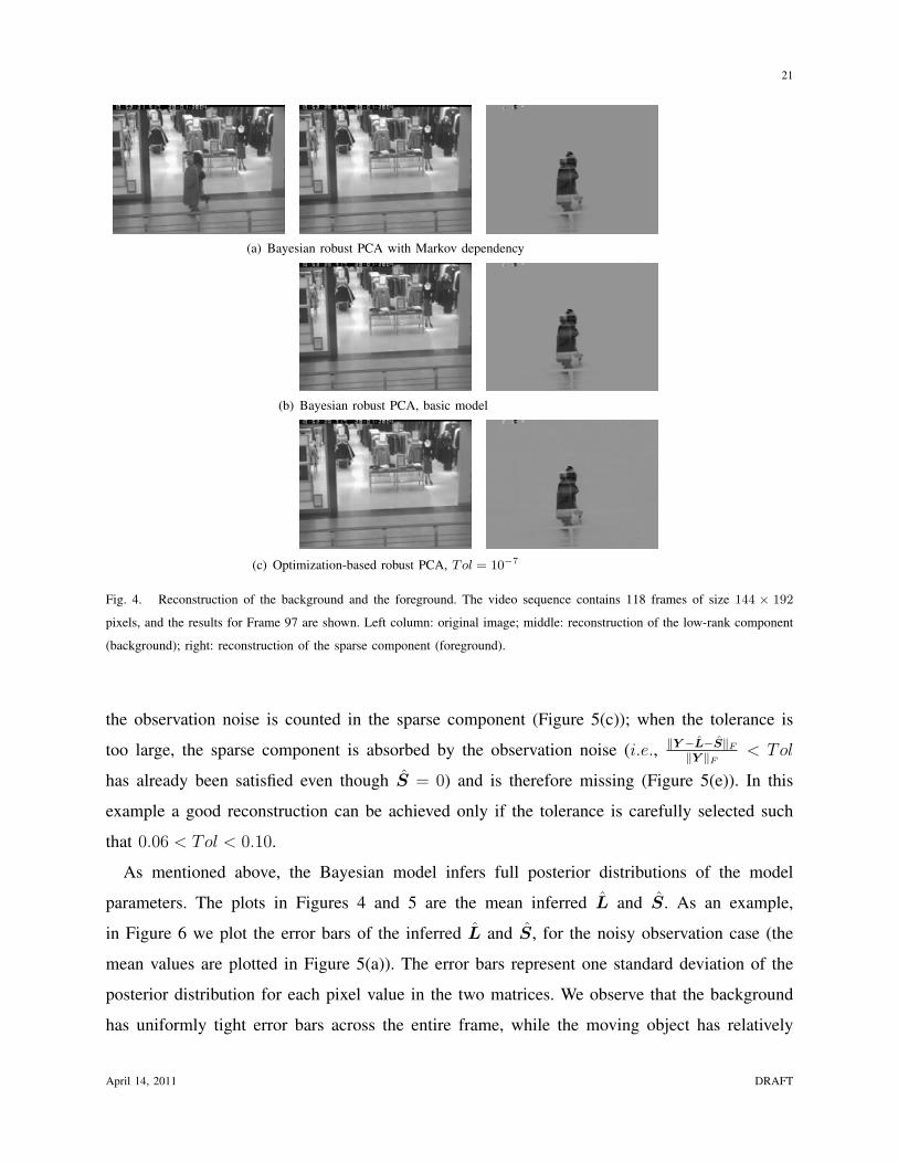
Fig. 4. Reconstruction of the background and the foreground. The video sequence contains 118 frames of size 144 × 192

pixels, and the results for Frame 97 are shown. Left column: original image; middle: reconstruction of the low-rank component

(background); right: reconstruction of the sparse component (foreground).

the observation noise is counted in the sparse component (Figure 5(c)); when the tolerance is

too large, the sparse component is absorbed by the observation noise (i.e., ∥Y −L−S∥F∥Y ∥F

< Tol

has already been satisfied even though S = 0) and is therefore missing (Figure 5(e)). In this

example a good reconstruction can be achieved only if the tolerance is carefully selected such

that 0.06 < Tol < 0.10.

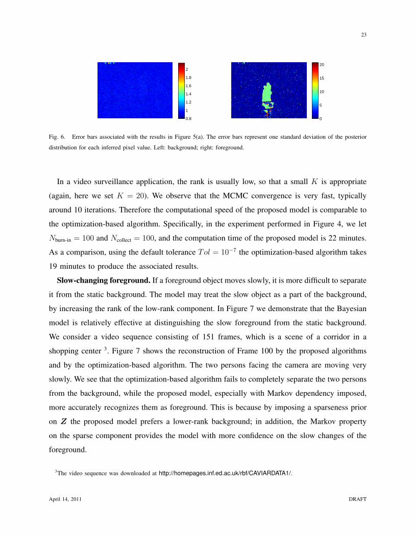
As mentioned above, the Bayesian model infers full posterior distributions of the model

parameters. The plots in Figures 4 and 5 are the mean inferred L and S. As an example,

in Figure 6 we plot the error bars of the inferred L and S, for the noisy observation case (the

mean values are plotted in Figure 5(a)). The error bars represent one standard deviation of the

posterior distribution for each pixel value in the two matrices. We observe that the background

has uniformly tight error bars across the entire frame, while the moving object has relatively


22



(c) Optimization-based robust PCA, Tol = 0.06

(d) Optimization-based robust PCA, Tol = 0.07

(e) Optimization-based robust PCA, Tol = 0.10

Fig. 5. Reconstruction of the background and the foreground under noisy observation. The additive white Gaussian noise has

standard deviation σ = 10. Left: original noisy image; middle: background reconstruction; right: foreground reconstruction.

large error bars, since it has more uncertainty.


23

0.8

1

1.2

1.4

1.6

1.8

2

0

5

10

15

20

Fig. 6. Error bars associated with the results in Figure 5(a). The error bars represent one standard deviation of the posterior

distribution for each inferred pixel value. Left: background; right: foreground.

In a video surveillance application, the rank is usually low, so that a small K is appropriate

(again, here we set K = 20). We observe that the MCMC convergence is very fast, typically

around 10 iterations. Therefore the computational speed of the proposed model is comparable to

the optimization-based algorithm. Specifically, in the experiment performed in Figure 4, we let

Nburn-in = 100 and Ncollect = 100, and the computation time of the proposed model is 22 minutes.

As a comparison, using the default tolerance Tol = 10−7 the optimization-based algorithm takes

19 minutes to produce the associated results.

Slow-changing foreground. If a foreground object moves slowly, it is more difficult to separate

it from the static background. The model may treat the slow object as a part of the background,

by increasing the rank of the low-rank component. In Figure 7 we demonstrate that the Bayesian

model is relatively effective at distinguishing the slow foreground from the static background.

We consider a video sequence consisting of 151 frames, which is a scene of a corridor in a

shopping center 3. Figure 7 shows the reconstruction of Frame 100 by the proposed algorithms

and by the optimization-based algorithm. The two persons facing the camera are moving very

slowly. We see that the optimization-based algorithm fails to completely separate the two persons

from the background, while the proposed model, especially with Markov dependency imposed,

more accurately recognizes them as foreground. This is because by imposing a sparseness prior

on Z the proposed model prefers a lower-rank background; in addition, the Markov property

on the sparse component provides the model with more confidence on the slow changes of the

foreground.

3The video sequence was downloaded at http://homepages.inf.ed.ac.uk/rbf/CAVIARDATA1/.


24



(c) Optimization-based robust PCA, Tol = 10−7

Fig. 7. Slow-changing foreground. The video contains 151 frames of size 144 × 192 pixels, and we show Frame 100. The

two persons closest to camera move very slowly. Left: original image; middle: background reconstruction; right: foreground

reconstruction.

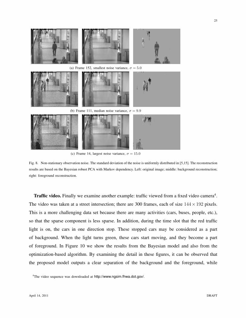
Non-stationary noise. Assume the noise variance varies across frames. We demonstrate that

the Bayesian model can adaptively learn the changes of the noise variance during the inference.

The model is modified as described in (12) for the noise term, and the noise precision γm,

for m = 1, ..,M , are inferred, each associated with one frame. We assume the noise standard

deviation σm is uniformly distributed in a range of [5, 15], i.e., σmi.i.d∼ U [5, 15],m = 1, ...,M ,

and the noise precision γm = 1/σ2m. The Bayesian model with Markov dependency is applied.

In Figure 8 we show the reconstruction of three frames: with smallest, median and largest

noise variance, respectively. Figure 9 plots the true σm and the inferred σm. We observe that the

proposed algorithm consistently obtains better estimate of noise variances across frames, without

any parameter tuning.


25

(a) Frame 152, smallest noise variance, σ = 5.0

(b) Frame 111, median noise variance, σ = 9.9

(c) Frame 14, largest noise variance, σ = 15.0

Fig. 8. Non-stationary observation noise. The standard deviation of the noise is uniformly distributed in [5,15]. The reconstruction

results are based on the Bayesian robust PCA with Markov dependency. Left: original image; middle: background reconstruction;

right: foreground reconstruction.

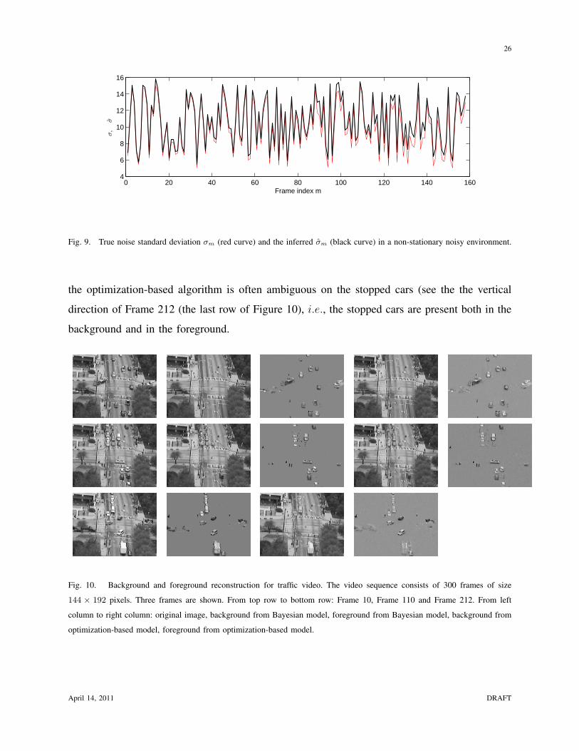
Traffic video. Finally we examine another example: traffic viewed from a fixed video camera4.

The video was taken at a street intersection; there are 300 frames, each of size 144×192 pixels.

This is a more challenging data set because there are many activities (cars, buses, people, etc.),

so that the sparse component is less sparse. In addition, during the time slot that the red traffic

light is on, the cars in one direction stop. These stopped cars may be considered as a part

of background. When the light turns green, these cars start moving, and they become a part

of foreground. In Figure 10 we show the results from the Bayesian model and also from the

optimization-based algorithm. By examining the detail in these figures, it can be observed that

the proposed model outputs a clear separation of the background and the foreground, while

4The video sequence was downloaded at http://www.ngsim.fhwa.dot.gov/.


26

0 20 40 60 80 100 120 140 1604

6

8

10

12

14

16

Frame index m

σ,

σ

Fig. 9. True noise standard deviation σm (red curve) and the inferred σm (black curve) in a non-stationary noisy environment.

the optimization-based algorithm is often ambiguous on the stopped cars (see the the vertical

direction of Frame 212 (the last row of Figure 10), i.e., the stopped cars are present both in the

background and in the foreground.

Fig. 10. Background and foreground reconstruction for traffic video. The video sequence consists of 300 frames of size

144 × 192 pixels. Three frames are shown. From top row to bottom row: Frame 10, Frame 110 and Frame 212. From left

column to right column: original image, background from Bayesian model, foreground from Bayesian model, background from

optimization-based model, foreground from optimization-based model.


27

C. Discussion

We also implemented the proposed Bayesian robust PCA model with variational Bayesian

(VB) inference, as discussed in Section IV. However, we found that the VB inference for the

model is often sensitive to model initialization (i.e., sensitive to local-optimal solutions). For the

toy example, we have to specify the initial values very carefully, sometimes even with a “trial-

and-error method”, to obtain the result comparable to that from the MCMC method, which

requires no tuning and may be initialized with randomly selected parameter values. In the real

examples, although the local-optimal-solution problem associated with VB is not as obvious as

that in the toy examples, it still exists. In addition, one important advantage of the VB method –

fast convergence – becomes less attractive in the real examples, because the MCMC method also

converges fast when the rank is low. Therefore, in practice it is felt that the Gibbs-sampler-based

implementation is the most useful for the proposed model.

VI. CONCLUSIONS

In [10], [17], [11] the authors developed a new robust PCA framework for analysis of matrices

with sparely distributed additive noise of arbitrary amplitude, and in [18] the model was extended

to consider small additive densely distributed noise. Under certain conditions the optimization-

based models have guarantees on model performance. This paper has sought to build on the

success of this research direction, by introducing a Bayesian formalism to this problem. The

Bayesian method has several attractive attributes: (i) it is robust to the densely distributed noise

and the noise statistics may be inferred based upon the data, with no tuning of hyperparameters;

(ii) the framework readily allows the addition of further constraints on the solution, for example

in the form of a Markov property on the sparse component, of particular interest for video

analysis, and similarly it allows the noise statistics to vary from frame to frame; (iii) for real

applications an MCMC-based computational implementation (Gibbs sampler) converges quickly

to an accurate mean solution, with computation time commensurate with that of the optimization-

based approach; and (iv) the Bayesian approach also yields “error bars” on the solution, of

potential interest for subsequent inferences (classification, tracking, etc.).

There are several directions of interest for future research. For example, in the video examples,

a fixed camera was assumed. However, there are clearly many applications for which one may

have a moving (e.g., hand-held) video camera. In this case, rather than assuming that the


28

background resides on a low-dimensional linear subspace (defined by the low-rank component),

it may be more appropriate to assume the background lives on a low-dimensional manifold. The

Bayesian formalism may be extended to infer the properties of the low-dimensional manifold

(e.g., by a mixture of factor analyzers, rather than by the single factor model associated with

the low-rank model).

REFERENCES

[1] C. Eckart and G. Young, “The approximation of one matrix by another of lower rank,” Psychometrika, vol. 1, pp. 211–218,

1936.

[2] J. B. Tenenbaum, V. de Silva, and J. C. Langford, “A global geometric framework for nonlinear dimensionality reduction,”

Science, vol. 290, pp. 2319–2323, 2000.

[3] J. Verbeek, “Learning nonlinear image manifolds by global alignment of local linear models,” IEEE Trans. Pattern Analysis

and Machine Intelligence, vol. 28, pp. 1236–1250, 2006.

[4] Netflix, Inc. The Netflix prize. http : //www.netflixprize.com/.

[5] I. T. Jolliffe, Principal Component Analysis. Springer-Verlag, 1986.

[6] C. M. Bishop, Pattern Recognition and Machine Learning. Springer-Verlag, 2006.

[7] J.-F. Cai, E. J. Candes, and Z. Shen, “A singular value thresholding algorithm for matrix completion,” SIAM Journal on

Optimization, vol. 20, pp. 1956–1982, 2008.

[8] R. Salakhutdinov and A. Mnih, “Probabilistic matrix factorization,” in Neural Information Processing Systems (NIPS),

2007.

[9] E. Candes and Y. Plan, “Matrix completion with noise,” IEEE Proc., pp. 925 – 936.

[10] J. Wright, Y. Peng, Y. Ma, A. Ganesh, and S. Rao, “Robust principal component analysis: Exact recovery of corrupted

low-rank matrices by convex optimization,” in Neural Information Processing Systems (NIPS), 2009.

[11] V. Chandrasekaran, S. Sanghavi, P. A. Parrilo, and A. S. Willsky, “Sparse and low-rank matrix decompositions,” in IFAC

Symposium on System Identification, 2009.

[12] P. J. Huber and E. M. Ronchetti, Robust Statistics, 2nd ed. Wiley, 2009.

[13] F. D. la Torre and M. J. Black, “A framework for robust subspace learning,” International Journal of Computer Vision,

vol. 54, pp. 117–142, 2003.

[14] R. Gnanadesikan and J. R. Kettenring, “Robust estimates, residuals, and outlier detection with multiresponse data,”

Biometrics, vol. 28, pp. 81–124, 1972.

[15] Q. Ke and T. Kanade, “Robust ℓ1 norm factorization in the presence of outliers and missing data by alternative convex

programming,” in IEEE Conf. Computer Vision and Pattern Recognition, 2005.

[16] M. A. Fischler and R. C. Bolles, “Random sample consensus: a paradigm for model fitting with applications to image

analysis and automated cartography,” Communications of the ACM, vol. 24, pp. 381–385, 1981.

[17] E. J. Candes, X. Li, Y. Ma, and J. Wright, “Robust principal component analysis?” Submitted to Journal of the ACM,

2009.

[18] Z. Zhou, J. Wright, X. Li, E. J. Candes, and Y. Ma, “Stable principal component pursuit,” in International Symposium on

Information Theory, 2010.


29

[19] M. E. Tipping and C. M. Bishop, “Probabilistic principal component analysis,” Journal of the Royal Statistical Society

Series B, vol. 61, pp. 611–622, 1999.

[20] J. Gao, “Robust ℓ1 principal component analysis and its Bayesian variational inference,” Neural Computation, vol. 20, pp.

555–578, 2008.

[21] J. Luttinen, A. Ilin, and J. Karhunen, “Bayesian robust PCA for incomplete data,” in International Conference on

Independent Component Analysis and Signal Separation, 2009.

[22] E. J. Candes and B. Recht, “Exact matrix completion via convex optimization,” Foundations of Computational Mathematics,

vol. 9, pp. 717–772, 2008.

[23] B. Recht, M. Fazel, and P. A. Parrilo, “Guaranteed minimum-rank solutions of linear matrix equations via nuclear norm

minimization,” Submitted to SIAM review, 2008.

[24] R. Salakhutdinov and A. Mnih, “Bayesian probabilistic matrix factorization using Markov chain Monte Carlo,” in

International Conference on Machine Learning, 2008.

[25] Y. J. Lim and Y. W. Teh, “Variational Bayesian approach to movie rating prediction,” in KDD Cup and Workshop, 2007.

[26] K. Yu, J. Lafferty, S. Zhu, and Y. Gong, “Large-scale collaborative prediction using a nonparametric random effects model,”

in International Conference on Machine Learning, 2009.

[27] N. D. Lawrence and R. Urtasun, “Non-lineaar matrix factorization with Gaussian processes,” in International Conference

on Machine Learning, 2009.

[28] S. Ji, Y. Xue, and L. Carin, “Bayesian compressive sensing,” IEEE Transactions on Signal Processing, vol. 56, pp. 2346–

2356, 2008.

[29] M. W. Seeger and H. Nickisch, “Compressed sensing and Bayesian experimental design,” in International Conference on

Machine Learning, 2008.

[30] D. Wipf, J. Palmer, and B. Rao, “Perspectives on sparse Bayesian learning,” in Advances in Neural Information Processing

Systems, 2004.

[31] L. He and L. Carin, “Exploiting structure in wavelet-based Bayesian compressive sensing,” IEEE Transactions on Signal

Processing, vol. 57, pp. 3488–3497, 2009.

[32] M. F. Duarte, M. B. Wakin, and R. G. Baraniuk, “Wavelet-domain compressive signal reconstruction using a hidden Markov

tree model,” in IEEE International Conference on Acoustics, Speech and Signal Processing (ICASSP), 2008.

[33] M. E. Tipping, “Sparse Bayesian learning and the relevance vector machine,” Journal of Machine Learning Research, pp.

211–244, 2001.

[34] P. Hoff, “Simulation of the matrix Bingham-von Mises-Fisher distribution, with applications to multivariate and relational

data,” J. Comp. Graph. Statistics, 2009.

[35] T. Park and G. Casella, “The Bayesian LASSO,” Journal of the American Statistical Association, vol. 103, pp. 681–686,

2008.

[36] J. Mairal, F. Bach, J. Ponce, and G. Sapiro, “Online dictionary learning for sparse coding,” in Proc. International Conference

on Machine Learning, 2009.

[37] C. P. Robert and G. Casella, Monte Carlo Statistical Methods, 2nd ed. New York: Springer, 2004.

[38] M. J. Beal, “Variational algorithms for approximate Bayesian inference,” Ph.D. dissertation, Gatsby Computational

Neuroscience Unit, University College London, 2003.

[39] Z. Lin, M. Chen, L. Wu, and Y. Ma, “The augmented lagrange multiplier method for exact recovery of corrupted low-rank

matrices,” University of Illinois at Urbana-Champaign, Tech. Rep. UILU-ENG-09-2215, 2009.


Documents

Bayesian Robust Principal Component Analysis - All …people.ee.duke.edu/~lcarin/LRS_09.pdf · 1 Bayesian Robust Principal Component Analysis 1;2Xinghao Ding, 1Lihan He and 1Lawrence