Bayesian Regularization Hedibert F. Lopeshedibert.org/wp-content/uploads/2015/12/BayesianRegularization.pdf · Bayesian Regularization Hedibert F. Lopes Insper - Institute of Education

Bayesian Regularization

Hedibert F. Lopes

Insper - Institute of Education and Research

August 4th, 2015

Hedibert Lopes (Insper) Brazilian School of Times Series and Econometrics August 3rd, 2015 1 / 38

1 Least absolute shrinkage and selection operator

2 Bridge regression and elastic net

3 Bayesian Lasso

4 Spike and slab variable selection

5 Horseshoe prior

6 Normal-gamma prior

7 Support vector machines

8 Sparse factor modelsCase 1: Constructing Economically Justified AggregatesCase 2: Exchange rates


Least absolute shrinkage and selection operator


In the linear regression set-up with p standardized regressors:

yi = x ′i β + εi ,

Tibshirani’s (1996) lasso solves the L1-penalization problem:

β = arg minβ

{l(β) + λ

p

∑j=1

|βj |}

.

Ridge regression: λ ∑pj=1 β2

j .

Variable seletion/shrinkage: The lasso does variable selection and shrinkage,whereas ridge regression, in contrast, only shrinks.

Bayesian interpretation: Maximum a posteriori under double-exponential prior.



Figure 2 of Tibshirani (1996)



Free advertisement



Other penalties

Breiman’s (1995) non-negative garrotte: minimize, with respect to cj ,

n

∑i=1

(yi −∑

j

cjxij βj

)2

subject to cj ≥ 0,p

∑j=1

cj ≤ t,

where βj are OLS.

Frank and Friedman’s (1993) bridge regression, where the penalty is

λp

∑j=1

|βj |γ,

with λ and γ estimated from the data.


Bridge regression and elastic net


Frank and Friedman’s (1993) Bridge regression generalizes both lasso and ridgeregression.

The bridge estimator can be viewed as the Bayes posterior mode under the prior

p(β|λ, q) ∝ exp{−λ|β|qq}.

Ridge regression: Gaussian priorLasso regression: Double-exponential prior.

Lasso + ridge: The elastic net penalty corresponds to a new prior given by

p(β|λ, α) ∝ exp{−λ(α|β|2 + (1− α)|β|1)},

a compromise between the Gaussian and Double-exponential priors.



Naıve elastic net

The naıve elastic net estimator is defined as

β = arg minβ{|y − X β|2 + λ1|β|1 + λ2|β|22}

Zou and Hastie (2005) argues that . . . the elastic net often outperforms the lasso,while enjoying a similar sparsity of representation. . . encourages a grouping. . . isparticularly useful when p is much bigger than n.



Theorem 2 of Zhou and Hastie (2005)

Given data (y ,X ) and (λ1, λ2) then the elastic net estimates β are given by

β = arg minβ

β′(X ′X + λ2I

1 + λ2

)β− 2y ′X β− λ1|β|1.

It is easy to see that

β(lasso) = arg minβ

β′(X ′X )β− 2y ′X β− λ1|β|1.

Also,X ′X + λ2I

1 + λ2= (1− γ)X ′X + γI ,

where γ = λ2/(1 + λ2).



Table 1 of Tibshirani (2011)


Bayesian Lasso

Bayesian Lasso

Park and Casella (2008) consider a fully Bayesian analysis using a conditionalLaplace prior specification of the form

p(β|σ2) ∝p

∏j=1

λ

2√

σ2exp{−λ|βj |/

√σ2}.

They show that “the Gibbs sampler for the Bayesian Lasso exploits the followingrepresentation of the Laplace distribution as a scale mixture of normals (with anexponential mixing density)” (Andrews and Mallows, 1974)

p(z |λ) = λ

2e−λ|z | =

∫ ∞

0N (z |0, τ2)E(τ2|λ2/2)dτ2

Related work: Fernandes and Steel (2000), Figueiredo (2003), Bae and Mallick(2004), Yuan and Lin (2005), Hans (2009,2010), Balakrishnan and Madigan(2010).The Bayesian bridge: Polson, Scott and Windle (2013)


Bayesian Lasso

Hierarchical model

The hierarchical representation of the full model is given by

y |µ,X , β, σ2 ∼ N(µ1n + X β, σ2In)

β|σ2, τ21 , . . . , τ2

p ∼ N(0, σ2Dτ)

σ2, τ21 , . . . , τ2

p ∼ p(σ2)dσ2p

∏j=1

λ2

2exp{−λ2τ2

j /2}dτ2j

where Dτ = diag(τ21 , . . . , τ2

p ).

The τ2j s are known as the local shrinkage parameters.

The full conditional distributions of τ2i s are inverse-Gaussian.

Note: Approximate analytical methods proposed by Tibshirani (1996) and Fanand Li (2001) fail to provide reasonable standard error estimates for theparameters estimated to be 0.


Bayesian Lasso

Elastic net & orthant normal prior

Hans (2011) shows that a modified version of the Zhou and Hastie’s (2005)elastic net penalty

p(β|α, λ, σ2) ∝ exp

[− λ

2σ2

{α|β|2 + (1− α)|β|1

}]can be rewritten as

p

∏j=1

{0.5N−

(βj |

1− α

2α,

σ2

λα

)+ 0.5N+

(βj |

1− α

2α,

σ2

λα

)}

where N− and N+ are properly normalized pdf for truncated normals. Or,

2−pΦ(−λ1

2σ√

λ2

)−p

∑z∈Z

N

(β| − λ1

2λ2z ,

σ2

λ2Ip

)1(β ∈ Oz ),

where Z = {−1, 1}p and Oz the orthant1 of of z ∈ Z .

1Analogue in n-dimensional Euclidean space of a quadrant (n=2) or an octant (n=3).Hedibert Lopes (Insper) Brazilian School of Times Series and Econometrics August 3rd, 2015 13 / 38

Spike and slab variable selection

Let us step back a bit (SSVS)

George and McCulloch (1993) is a seminal paper in the Bayesian literatureregarding variable selection via sparsity:

βi |γi ∼ (1− γi )N(0, τ2i ) + γiN(0, c2

i τ2i ).

Prior of γ:

p(γ) =

∏ pγii (1− pi )

(1−γi )

12p

ω|γ|Cp,|γ|

See also George and McCulloch (1997), who describes and compares varioushierarchical mixture prior formulations of variable selection uncertainty in normallinear regression models.


Spike and slab variable selection

Spike and slab approaches

By a spike and slab model, Ishwaran and Rao (2005) mean a Bayesian modelspecified by the following prior hierarchy:

yi |xi , β, σ2 ∼ N(x ′i β, σ2)

(β|γ) ∼ N(0, Γ)γ ∼ π(dγ)

σ2 ∼ µ(dσ2)

The literature designs hierarchical priors over parameter and model spaces.2

Gibbs sampling is used to identify promising models.

The choice of priors is often tricky.

Barbieri and Berger (2004) have shown that

in many circumstances the high frequency model is not the optimalpredictive model and that the median model is predictively optimal.

2Mitchell and Beauchamp (1988), Chipman (1996), Clyde, DeSimone and Parmigiani (1996),Geweke (1996), Kuo and Mallick (1998), Chipman, George and McCulloch (2001), O’Hara andSillanpaa (2009).


Horseshoe prior

The horseshoe prior

Carvalho, Polson and Scott (2010) propose a hierarchical prior as follows:

θi |λi ∼ N(0, λ2i )

λi |τ ∼ C+(0, τ)

τ|σ ∼ C+(0, σ),

where C+(0, a) is a standard half-Cauchy distribution

Horseshoe prior: When σ2 = τ2 = 1:

E (θi |y) =∫ 1

0(1− κi )yip(κi |y)dκi = {1− E (κi |y)}yi ,

where κi = 1/(1 + λ2i ). E (κi |y) is the amount of shrinkage towards zero.

The half-Cauchy prior on λi implies a horseshoe-shaped Be(1/2, 1/2) prior forthe shrinkage coefficient κi .


Horseshoe prior

Horseshoe prior


Normal-gamma prior

Normal-gamma prior Griffin and Brown (2010)

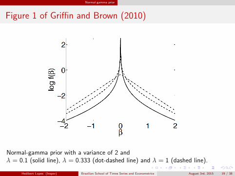
The normal-gamma distribution arises by assuming that the mixing distribution ina scale mixture of normals (SMN) has the density g(x) = Ga(x |λ, 1/(2γ2)):

p(βi ) =1√

2π2λ−1/2γλ+1/2Γ(λ)|βi |λ−1/2Kλ−1/2(|βi |/γ),

where K is the modified Bessel function of the third kind.

The variance of βi is 2λγ2 and the excess kurtosis is 3/λ.

Small λ:

Large mass close to zero.

Heavy tails.


Normal-gamma prior

Figure 1 of Griffin and Brown (2010)

Normal-gamma prior with a variance of 2 andλ = 0.1 (solid line), λ = 0.333 (dot-dashed line) and λ = 1 (dashed line).


Normal-gamma prior

The distribution is a member of the generalized hyperbolic family(Barndorff-Nielsen and Blaesild 1981).

The prior was considered by Griffin and Brown (2007), but the shape of thedensity made it difficult to obtain MAP estimates.

More recently, Caron and Doucet (2008) have looked at MAP estimation anddrawn a link to Levy processes.

See also Griffin and Brown (2013).


Support vector machines


Polson and Scott (2011) introduce a latent variable representation of regularizedsupport vector machines3 (SVM) that enables EM, ECME or MCMC algorithmsto provide parameter estimates. See also Tipping (2001).

The Lα-norm regularized support vector classifier chooses a set of coefficients β tominimize the objective function

dα(β, µ) =n

∑i=1

max(1− yix′i β, 0) + ν−α

k

∑j=1

|βj /σj |α,

where σj is the standard deviation of the j ’th element of x and ν is a tuningparameter.

Minimizing the above equation is equivalent to finding the mode of thepseudo-posterior distribution p(β|ν, α, y) defined by

p(β|ν, α, y) ∝ exp{−dα(β, ν)) ∝ Cα(ν)L(y |β)p(β|ν, α).

3Binary classifiers that are often used with extremely high dimensional covariates.Hedibert Lopes (Insper) Brazilian School of Times Series and Econometrics August 3rd, 2015 21 / 38


Local shrinkage rules and Levy processes

Polson and Scott (2012) use Levy processes to generate joint prior distributionsfor a location parameter β = (β1, . . . , βp) as p grows large.

This generalizes the class of local-global shrinkage rules based on scale mixtures ofnormals. See also Polson and Scott (2011).


Sparse factor models


The basic, most common, linear and Gaussian factor structure is

yi |fi ∼ N(βfi , Σ)fi ∼ N(0,H)

where Σ = diag(σ21 , . . . , σ2

p ) and H = diag(h1, . . . , hk ), such that

Var(yi ) = βHβ′ + Σ.

Sparsity:West (2003), Carvalho et al. (2008) and Fruhwirth-Schnatter and Lopes (2009)

βij ∼ (1− πij )δ0(βij ) + πijN(βij |0, τj )

πij ∼ (1− ρj )δ0(πij ) + ρjBe(πij |ajmj , aj (1−mj )),

where Be(am, a(1−m) is a beta with mean m and precision a.



Figure 1(a) of Carvalho et al. (2008)

See Lucas et al. (2006), Knowles and Ghahramani (2011), Ma and Zhao (2012),Runcie and Mukherjee (2013), Mayrink and Lucas (2013), Gao, Brown andEngelhardt (2013) and Zhao, Gao, Mukherjee and Engelhardt (2014) foradditional contributions related to genomics.

Pati, Bhattacharya, Pillai and Dunson (2014)



Sparse Factor models in Econometrics

Fruhwirth-Schnatter and Lopes (2009/2015)Parsimonious/Sparse Bayesian Factor Analysis when the Number of Factors is Unknown

Conti, Heckman, Lopes and Piatek (2011)Constructing Economically Justified Aggregates: An Application to the Early Origins ofHealth

Hahn and Lopes (2013)4 Factor model shrinkage for linear instrumental variable analysiswith many instruments

Kastner, Fruhwirth-Schnatter and Lopes (2015)Sparse Bayesian Latent Factor Stochastic Volatility Models for High-DimensionalFinancial Time Series

4Hahn, Carvalho and Mukherjee (2013)Hedibert Lopes (Insper) Brazilian School of Times Series and Econometrics August 3rd, 2015 25 / 38

Sparse factor models Case 1: Constructing Economically Justified Aggregates

Case 1: Constructing Economically Justified Aggregates

Application to the 1970 British Cohort Study to analyze the effect of childcognition, mental/physical health on educational choices and adult economic andhealth outcomes.

A survey of all babies born (alive or dead) after the 24th week of gestation from00.01 hours on Sunday, 5th April to 24.00 hours on Saturday, 11 April, 1970 inEngland, Scotland, Wales and Northern Ireland.

Follow-ups (so far): 1975, 1980, 1986, 1996, 2000, 2004, 2008.

Background characteristics:

Cognitive, mental, physical health measurements (age 10)Education and adult outcomes (age 30)

Sample size: 5,105 women and 5,420 men.Hedibert Lopes (Insper) Brazilian School of Times Series and Econometrics August 3rd, 2015 26 / 38


Overall Model



Overall model

M?1

...M?

QD?

Y ?01

Y ?11...

Y ?0S

Y ?1S

=

α′1 0...

...α′Q 0

α′D α′Zα′01 0α′11 0

......

α′0S 0α′1S 0

(XZ

)+

β′M1...

β′MQ

β′Dβ′01β′11

...β′0Sβ′1S

θ +

εM1...

εMQ

εDε01

ε11...

ε0Sε1S

,









Two main latent factors

ADHD: Attention Deficit Hyperactivity DisorderIt is loaded highly by items which are related to the child’s inability to payattention or to the child’s hyperactivity, as perceived by the teacher.

IQ: Cognitive AbilityIt is loaded highly by cognitive ability tests.


Sparse factor models Case 2: Exchange rates

Case 2: Exchange rates

EUR exchange rates. Data stems from the European Central Banks StatisticalData Warehouse and comprises T = 3140 observations of 20 currencies rangingfrom January 3, 2000 to April 4, 2012.



Factor stochastic volatility model

The basic FSV model is written as

yt |ft ∼ N(βft , Σt)

ft ∼ N(0,Ht)

where

Σt = diag(σ21t , . . . , σ2

pt)

Ht = diag(σ2p+1,t , . . . , σ2

p+k,t),

andlog σ2

it | log σ2i ,t−1 ∼ N(µi + φi (log σ2

i ,t−1 − µi ), τ2i )

for i = 1, . . . , p + k.

Key features:Griffin and Brown’s (2010) Normal-Gamma prior on β.Rue’(2001) and McCausland, Miller, and Pelletier’s (2011) All WithOut aLoop (AWOL) sampling.Yu and Meng’s (2011) Ancillarity-Sufficiency Interweaving Strategy (ASIS)



Commonalities



Time-varying Covariances



References

Andrews and Mallows (1974) Scale Mixtures of Normal Distributions. JRSS-B, 36, 99-102.Bae and Mallick (2004) Gene Selection Using a Two-Level Hierarchical Bayesian Model. Bioinformatics, 20, 3423-3430.Balakrishnan and Madigan (2010) Priors on the variance in sparse Bayesian learning: the demi-Bayesian lasso. In Frontiers of Statistical Decision Makingand Bayesian Analysis: In Honor of James O. Berger by Chen, Muller, Sun, and Ye.Barbieri and Berger (2004) Optimal predictive model selection. Annals of Statistics, 32, 870-897.Barndorff-Nielsen and Blaesild (1981) Hyperbolic distributions and ramifications: contributions to the theory and applications. In Statistical Distributionsin Scientific Work, Vol. 4, 19-44. Dorderecht: Reidal.Breiman (1995) Better subset selection using the non-negative garotte. Technometrics, 37, 738-754.Caron and Doucet (2008) Sparse Bayesian nonparametric regression. International Conference on Machine Learning (ICML 2008), Helsinki, Finland, July2008.Carvalho, Chang, Lucas, Nevins, Wang and West (2008)High-dimensional sparse factor modeling: Applications in gene expression genomics. JASA, 103, 1438-1456.Chipman (1996). Bayesian variable selection with related predictors. Canadian Journal of Statistics, 24, 17-36.Chipman, George and McCulloch (2001) The practical implementation of Bayesian model selection. In Model Selection (P. Lahiri, ed.) 65-134. IMS,Beachwood, OH.Clyde, DeSimone and Parmigiani (1996) Prediction via orthogonalized model mixing. JASA, 91, 1197-1208.Fan and Li (2001) Variable selection via non-concave penalized likelihood and its oracle properties. JASA, 96, 1348-1360.Fernandez and Steel (2000) Bayesian regression analysis with scale mixtures of normals. Econometric Theory, 16, 80-101.Figueiredo (2003) Adaptive Sparseness for Supervised Learning. IEEE Transactions on Pattern Analysis and Machine Intelligence, 25, 1150-1159.Frank and Friedman (1993) A statistical view of some Chemometrics regression tools. Technometrics, 35, 109-148.Fu (1998) Penalized regression: the bridge versus the lasso. JCGS, 7, 397-416.Gao, Brown and Engelhardt (2013) A latent factor model with a mixture of sparse and dense factors to model gene expression data with confoundingeffects. http://arxiv.org/abs/1310.4792

George (2000) The variable selection problem. JASA, 95, 1304-1308.George and McCulloch (1993) Variable selection via Gibbs sampling. JASA, 88, 881-889.George and McCulloch (1997) Approaches for Bayesian variable selection. Statistica Sinica, 7, 339-373.Geweke (1996) Variable selection and model comparison in regression. In Bayesian Statistics 5, (J. M. Bernardo, J. O. Berger, A. P. Dawid and A. F. M.Smith, eds.) 609-620. Oxford Univ. Press, New York.Griffin and Brown (2010) Inference with normal-gamma prior distributions in regression problems. Bayesian Analysis, 5, 171-188.Griffin and Brown (2012) Structuring shrinkage: some correlated priors for regression. Biometrika, 99, 481-487.Griffin and Brown (2013) Some priors for sparse regression modelling. Bayesian Analysis, 8, 691-702.Hahn, Carvalho and Mukherjee (2013) Partial Factor Modeling: Predictor-Dependent Shrinkage for Linear Regression, JASA, 108, 999-1008.Hans (2009) Bayesian lasso regression. Biometrika, 96, 835-845.Hans (2010) Model uncertainty and variable selection in Bayesian lasso regression. Statistics and Computing, 20, 221-229.



References

Knowles and Ghahramani (2011) Nonparametric Bayesian sparse factor models with application to gene expression modeling. The Annals of AppliedStatistics, 5, 1534-1552.Kuo and Mallick (1998) Variable selection for regression models. Sankhya Series B, 60, 65-81.Lucas, Carvalho, Wang, Bild, Nevins and West (2006) Sparse statistical modelling in gene expression genomics. In Bayesian Inference for Gene Expressionand Proteomics (Muller, Do and Vannucci, eds.) 155-176. Cambridge Univ. Press, Cambridge.Ma and Zhao (2012) FacPad: Bayesian sparse factor modeling for the inference of pathways responsive to drug treatment. Bioinformatics, 28, 2662-2670.Mayrink and Lucas (2013) Sparse latent factor models with interactions: analysis of gene expression data. The Annals of Applied Statistics, 7, 799-822.McCausland, Miller and Pelletier (2011) Simulation smoothing for statespace models: A computational efficiency analysis. CSDA, 55, 199-212.Mitchell and Beauchamp (1988) Bayesian variable selection in linear regression. JASA, 83, 1023-1036.O’Hara and Sillanpaa (2009) A Review of Bayesian Variable Selection Methods: What, How and Which. Bayesian Analysis, 4, 85-118.Pati, Bhattacharya, Pillai and Dunson (2014) Posterior contraction in sparse Bayesian factor models for massive covariance matrices. The Annals ofStatistics, 42, 1102-1130.Polson and Scott (2011) Data Augmentation for Support Vector Machines. Bayesian Analysis, 6, 1-24.Polson and Scott (2011) Shrink globally, act locally: sparse Bayesian regularization and prediction. In Bayesian Statistics 9 (eds Bernardo, Bayarri, Berger,Dawid, Heckerman, Smith and West). Oxford: Oxford University Press.Polson and Scott (2012) Local shrinkage rules, Levy processes and regularized regression. JRSS-B, 74, 287-311.Polson, Scott and Windle (2013) The Bayesian bridge. JRSS-B, 76, 713-733.Rue (2001) Fast sampling of Gaussian Markov random fields with applications. JRSS-B, 63, 325-338.Runcie and Mukherjee (2013) Dissecting High-Dimensional Phenotypes with Bayesian Sparse Factor Analysis of Genetic Covariance Matrices. Genetics,194, 753-767.Tibshirani (1996) Regression shrinkage and selection via the lasso. JRSS-B, 58, 267-288.Tibshirani (2011) Regression shrinkage and selection via the lasso: a retrospective. JRSS-B, 73, 273-282.Tipping (2001) Sparse Bayesian Learning and the Relevance Vector Machine. Journal of Machine Learning Research, 1, 211-244.West (2003) Bayesian factor regression models in the large p, small n paradigm. In Bayesian Statistics 7, (J. Bernardo, M. Bayarri, J. Berger, A. Dawid, D.Heckerman, A. Smith and M.West, eds.), Oxford U.K.: Oxford University Press, pp. 723-732.Yu and Meng (2011) To Center or Not to Center: That Is Not the QuestionAn AncillaritySufficiency Interweaving Strategy (ASIS) for Boosting MCMCEfficiency. JCGS, 20, 531-570.Yuan and Lin (2005) Efficient Empirical Bayes Variable Selection and Estimation in Linear Models. JASA, 100, 1215-1225.Zhao, Gao, Mukherjee and Engelhardt (2014) Bayesian group latent factor analysis with structured sparse priors http://arxiv.org/abs/1411.2698

Zou and Hastie (2005) Regularization and variable selection via the elastic net. JRSS-B, 67, 301-320.


Documents

Bayesian Regularization Hedibert F. Lopeshedibert.org/wp-content/uploads/2015/12/BayesianRegularization.pdf · Bayesian Regularization Hedibert F. Lopes Insper - Institute of Education