Bayesian Policy Gradient Algorithms - University of …ppoupart/ICML-07-tutorial-slides/icml07... · Bayesian Policy Gradient Algorithms. ... GP to define a prior distribution over

Bayesian Methods in Reinforcement Learning ICML 2007

Bayesian Policy Gradient Algorithms


Reinforcement learning

RL: A class of learning problems in which an agent interacts with an unfamiliar, dynamic and stochastic environment

Goal: Learn a policy to maximize some measure of long-term reward

Interaction: Modeled as a MDP or a POMDP

Environment

Action

State

Reward

RL&AI Laboratory . Department of Computing Science . University of Alberta RL&AI Laboratory . Department of Computing Science . University of Alberta

Markov decision process (MDP)

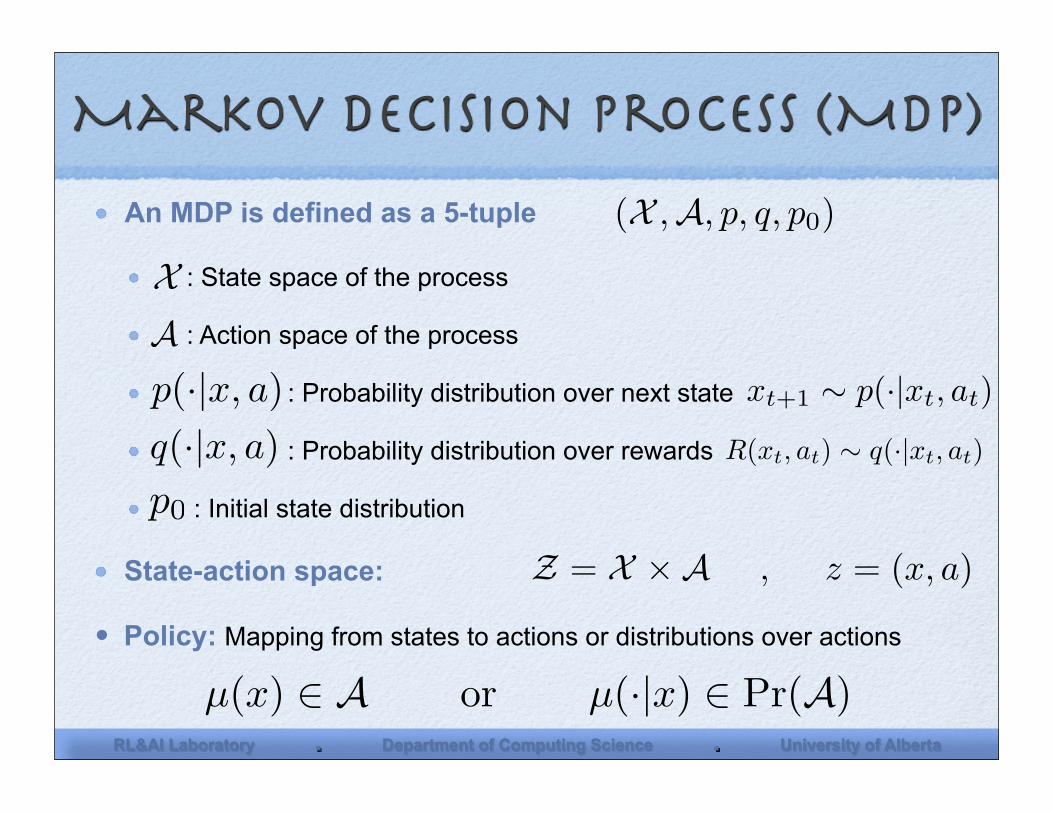
An MDP is defined as a 5-tuple

: State space of the process

: Action space of the process

: Probability distribution over next state

: Probability distribution over rewards

: Initial state distribution

State-action space: Z = X !A , z = (x, a)

XA

q(·|x, a)

(X ,A, p, q, p0)

p0

p(·|x, a) xt+1 ! p(·|xt, at)

• Policy: Mapping from states to actions or distributions over actions

µ(x) ! A or µ(·|x) ! Pr(A)

R(xt, at) ! q(·|xt, at)


Value FunctionAlgorithms

SARSAQ-learning

Value Iteration

Actor-CriticAlgorithms

Policy SearchAlgorithms

PEGASUSGenetic Algorithms

Sutton, et al. 2000Konda & Tsitsiklis 2000

Peters, et al. 2005Bhatnagar, Ghavamzadeh, Sutton 2007

Reinforcement learning solutions

Policy GradientAlgorithms

Sutton et al. 2000Konda 2000



V µ(x) = E

! !"

t=0

!tr(xt, at)|x0 = x

#

Qµ(x, a) = E

! !"

t=0

!tr(xt, at)|x0 = x, a0 = a

#


Policy Performance

• System Path: ! = (x0, a0, x1, a1, . . . , xT!1, aT!1, xT )

• Probability of a Path: Pr(!|µ) = p0(x0)T!1!

t=0

µ(at|xt)p(xt+1|xt, at)

• Return of a Path: D(!) =T!1!

t=0

"tR(xt, at)

• Expected Return: !(µ) = E[D(")] =!

D(") Pr("|µ)d"

• Expected Return: !(µ) =!

"(x, a;µ)R(x, a)dxda


Policy gradient methods

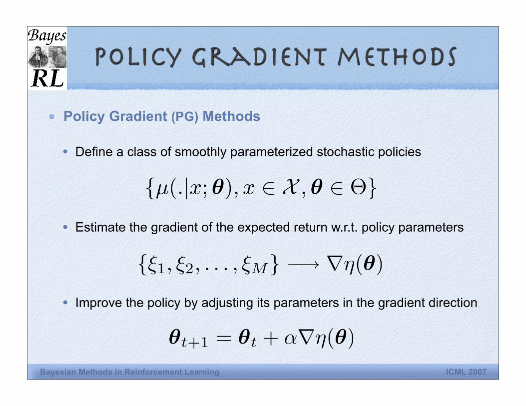
Policy Gradient (PG) Methods

{µ(.|x;!), x ! X ,! ! !}• Define a class of smoothly parameterized stochastic policies

{!1, !2, . . . , !M} !" #"(!)

• Estimate the gradient of the expected return w.r.t. policy parameters

!t+1 = !t + !!"(!)

• Improve the policy by adjusting its parameters in the gradient direction


Gradient estimation

• Score Function

u(!) =!Pr(!;!)Pr(!;!)

= ! log Pr(!;!) =T!1!

t=0

! log µ(at|xt;!)

• Expected Return !(!) = !(µ(·|·;!)) =!

D(") Pr(";!)d"

• Score Function or Likelihood Ratio Method

!!(!) =!

D(")!Pr(";!)Pr(";!)

Pr(";!)d"

• Monte-Carlo (MC) Estimation

!!(!) =1M

M!

i=1

D("i)Ti!1!

t=0

! log µ(at,i|xt,i;!)


shortcomings of policy gradient methods

Examples of PG Algorithms

Class of REINFORCE algorithms (Williams 1992)

Extending to infinite-horizon MDPs and POMDPs (Kimura et al. 1995,

Marbach 1998, Baxter & Bartlett 2001)

Shortcomings of PG Algorithms

MC estimates of the gradient have high variance

Require excessive number of samples

Slow convergence

Inefficient use of data


Improving policy gradient Algorithms

Speeding up the PG Algorithms

Using discount factor (Marbach 1998, Baxter & Bartlett 2001)

Using a baseline (Williams 1992, Sutton et al. 2000)

Natural Gradient (Kakade 2002, Bagnell & Schneider 2003, Peters et al. 2003)

Contributions of this Work

A Bayesian framework for policy gradient

Lower variance - Less samples - Faster convergence

Covariance of estimate is provided at little extra cost


Bayesian quadrature (0’hagan 1991)

Integral Evaluation

MC Estimate

Bayesian Quadrature

Model as a Gaussian Process (GP)

A set of samples is observed DM = {(xi, yi)}Mi=1

! =!

F (x)p(x)dx

!MC =1M

M!

i=1

F (xi)

F F (·) ! N{f0(·), k(·, ·)}

E[F (x)] = f0(x) , Cov[F (x), F (x!)] = k(x, x!)


Bayesian Quadrature

Posterior mean and covariance of are computedf

!0 =!

f0(x)p(x)dx , zM =!

kM (x)p(x)dx , z0 =! !

k(x, x!)p(x)p(x!)dxdx!

Bayesian quadrature (0’hagan 1991)

E[F (x)|DM ] = f0(x) + kM (x)!CM (yM ! f0)

Cov[F (x), F (x!)|DM ] = k(x, x!)! kM (x)"CMkM (x!)

Posterior mean and variance of are computed as!

E[!|DM ] =!

E[F (x)|DM ]p(x)dx = !0 + z!MCM (yM ! f0)

Var[!|DM ] =! !

Cov[F (x), F (x!)|DM ]p(x)p(x!)dxdx! = z0 + z"MCMzM


• Model 1:

p(!;!)F (!;!)

Bayesian policy gradient(Ghavamzadeh & Engel, NIPS 2006)

k(!i, !j) = (1 + u(!i)!G"1u(!j))2 !"!

(zM )i = 1 + u(!i)!G"1u(!j)z0 = 1 + n

zM =!

kM (!) Pr(!;!)d! , z0 =! !

k(!, !!) Pr(!;!) Pr(!!;!)d!d!!

E(!!(!)|DM ) = Y MCMzM , Cov(!!(!)|DM ) = (z0 " z!MCMzM )I

• Gradient of the performance measure

!!(!) =!

D(")! log Pr(";!) Pr(";!) d"


• Model 2:

p(!;!)F (!;!)

E(!!(!)|DM ) = ZMCMyM , Cov(!!(!)|DM ) = Z0 "ZMCMZ!M

ZM =!

kM (!)!!Pr(!;!)d! , Z0 =! !

k(!, !")!Pr(!;!)!Pr(!";!)!d!d!"

k(!i, !j) = u(!i)!G"1u(!j) !"!

ZM = UM = [u(!1), . . . ,u(!M )]Z0 = G!UMCMU!

M


• Gradient of the performance measure

!!(!) =!

D(") ! log Pr(";!) Pr(";!) d"


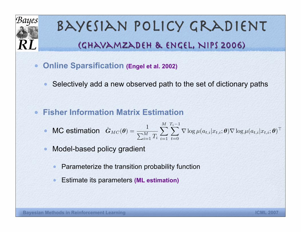
Fisher Information Matrix Estimation

MC estimation

Model-based policy gradient

Parameterize the transition probability function

Estimate its parameters (ML estimation)

GMC(!) =1

!Mi=1 Ti

M"

i=1

Ti!1"

t=0

! log µ(at,i|xt,i;!)! log µ(at,i|xt,i;!)"

Online Sparsification (Engel et al. 2002)

Selectively add a new observed path to the set of dictionary paths



Linear Quadratic regulator

System

Initial State

State Transition

Reward

Policy

Actions

Parameters

x0 ! N (0.3, 0.001)

at ! µ(.|xt;!) = N (!xt,"2)

! = (!, ")!

xt+1 = xt + at + nx , nx ! N (0, 0.01)

Rt = x2t + 0.1a2

t


0 20 40 60 80 100100

101

102

Number of Paths

Mea

n Ab

s Ang

ular E

rror (

deg)

MCBQ

0 20 40 60 80 100100

101

102

Number of Paths

Mea

n Ab

s Ang

ular E

rror (

deg)

MCBQ

0 20 40 60 80 100102

103

104

105

106

Number of Paths

Mea

n Sq

uare

d Er

ror

MCBQ

0 20 40 60 80 100103

104

105

Number of Paths

Mea

n Sq

uare

d Er

ror

MCBQ


0 20 40 60 80 100

100

101

Number of Updates (Sample Size = 5)

Aver

age

Expe

cted

Retu

rn

MCBPGOptimal

0 20 40 60 80 100

100

101


Aver

age

Expe

cted

Retu

rn

MCBPGOptimal

0 20 40 60 80 100

100

101


Aver

age

Expe

cted

Retu

rn

MCBPGOptimal

0 20 40 60 80 100

100

101


Aver

age

Expe

cted

Retu

rn

MCBPGOptimal


0 20 40 60 80 10010!0.5

10!0.4

10!0.3

10!0.2

10!0.1


Aver

age

Expe

cted

Retu

rn

MCBPGBPG!MLBPG!MCOptimal

0 20 40 60 80 10010!0.5

10!0.4

10!0.3

10!0.2

10!0.1


Aver

age

Expe

cted

Retu

rn


0 20 40 60 80 10010!0.5

10!0.4

10!0.3

10!0.2

10!0.1


Aver

age

Expe

cted

Retu

rn



Bayesian Actor-Critic Algorithms


Actor-Critic

Environment

ActorPolicy

Policy Gradient

CriticValue Function

TD-Learning

State Action

Reward

ControlPrediction

x a

r(x, a)

z = (x, a)


Bayesian Actor-Critic(Ghavamzadeh & Engel, ICML 2007)

• Performance measure

Actor

GP• Gradient of the performance measure

!!(!) =!

"(z;!) ! log µ(a|x;!) Q(z;!) dz =!

g(z;!) Q(z;!) dz

Cov(!!(!)|Dt) =! !

g(z;!) Cov(Q(z;!), Q(z!;!)|Dt) g(z!;!)! dz dz!

E(!!(!)|Dt) =!

g(z;!) E(Q(z;!)|Dt) dz

• Posterior moments of gradient

!(!) =!

"(z;!)R(z)dz


Critic• GPTD (Engel, Mannor, & Meir 2003, 2005)

E(Q(z;!)|Dt) = kt(z)!"t

Cov(Q(z;!), Q(z!;!)|Dt) = k(z,z!)! kt(z)!Ctkt(z!)!

k(z,z!) = kx(x, x!) + kF (z,z!) !"!

U t = [u(z0), . . . ,u(zt)]V = G

u(z)!G"1u(z!)=

U t =!

g(z;!)kt(z)!dz , V =! !

g(z;!)k(z,z!)g(z!;!)!dzdz!

E(!!(!)|Dt) = U t"t , Cov(!!(!)|Dt) = V "U tCtU!t

Actor

Bayesian Actor-Critic(Ghavamzadeh & Engel, ICML 2007)


System

State Space

Action Space

Initial State - Terminal State

Cost

Policy

Actions

Parameters

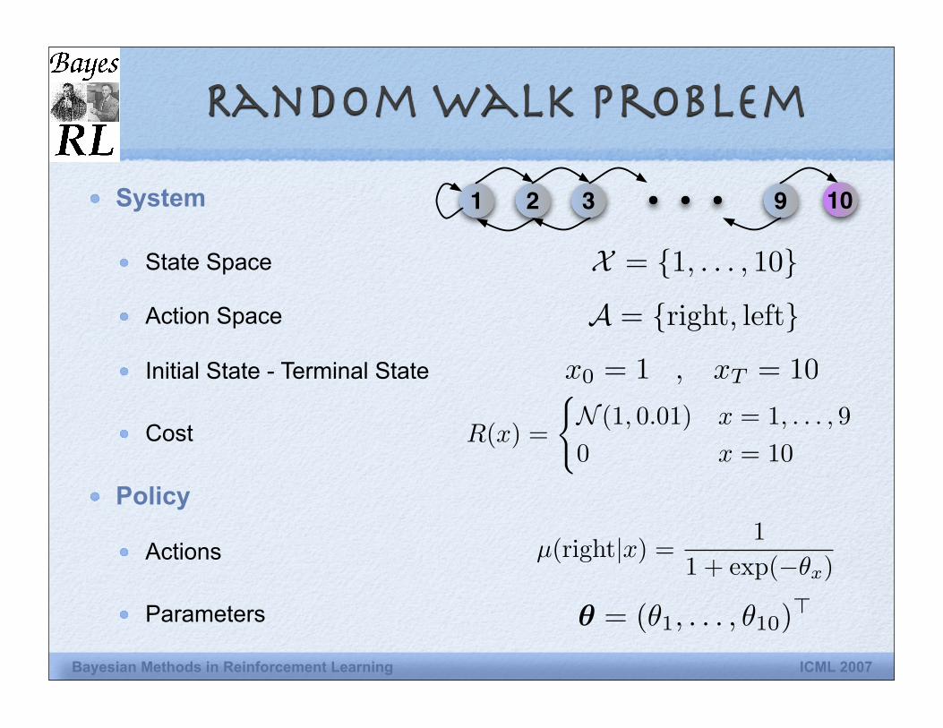
Random Walk Problem

X = {1, . . . , 10}

A = {right, left}

x0 = 1 , xT = 10

µ(right|x) =1

1 + exp(!!x)

! = (!1, . . . , !10)!

9321 10

R(x) =

!N (1, 0.01) x = 1, . . . , 90 x = 10


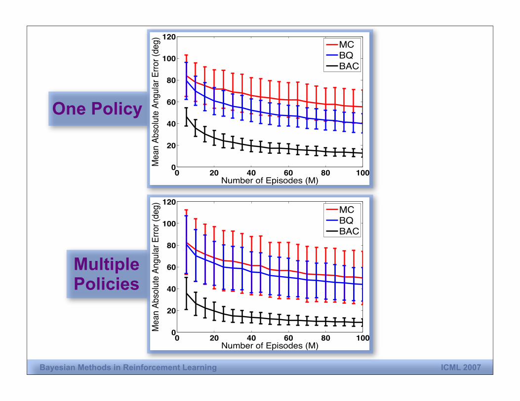
One Policy

MultiplePolicies

0 20 40 60 80 1000

20

40

60

80

100

120

Number of Episodes (M)

Mea

n Ab

solut

e An

gular

Erro

r (de

g)

MCBQBAC

0 20 40 60 80 1000

20

40

60

80

100

120

Number of Episodes (M)

Mea

n Ab

solut

e An

gular

Erro

r (de

g)

MCBQBAC


0 100 200 300 400 50010!2

10!1

100

101

102

Number of Policy Updates (M = 1)

!(")

! !

*

MCBPGBAC

0 100 200 300 400 50010!2

10!1

100

101

102


!(")

! !

*

MCBPGBAC

0 100 200 300 400 50010!2

10!1

100

101

102


!(")

! !

*

MCBPGBAC


BPG & BAC Comparison

Bayesian Policy Gradient (BPG) (Ghavamzadeh & Engel, 2006)

Basic observable unit: complete system trajectory

Allow handling non-Markovian systems (e.g. partial observability, Markov games)

Bayesian Actor-Critic (BAC)

Basic observable unit: individual state-action-reward transitions (Markov property)

Reduce the variance of the gradient estimates

Allow handling systems with long and/or variable-length trajectories


Summary

An alternative approach (Bayesian) to conventional MC-based (frequentist) policy gradient estimation procedure

Less variance

Less number of samples

Faster convergence

Natural gradient and gradient covariance are provided at little extra cost

GP to define a prior distribution over the gradient of the expected return

Compute its posterior conditioned on the observed data


future work

Using gradient covariance

Risk-aware selection of the update step-size and direction

Termination condition

Combining with MDP model estimation (Model-Based BAC Algorithms)

Transfer of learning between different policies

More data efficient PG algorithms

More flexibility in kernel function selection

Non-parametric policies

Second order updates - how to estimate the Hessian?

More challenging problems (e.g. control of an octopus arm)

Documents

Bayesian Policy Gradient Algorithms - University of …ppoupart/ICML-07-tutorial-slides/icml07... · Bayesian Policy Gradient Algorithms. ... GP to define a prior distribution over