Embed Size (px)
Citation preview

Bayesian Nonparametrics:Dirichlet Process
Yee Whye TehGatsby Computational Neuroscience Unit, UCL
http://www.gatsby.ucl.ac.uk/~ywteh/teaching/npbayes2012

Dirichlet Process
• Cornerstone of modern Bayesian nonparametrics.
• Rediscovered many times as the infinite limit of finite mixture models.
• Formally defined by [Ferguson 1973] as a distribution over measures.
• Can be derived in different ways, and as special cases of different processes.
• Random partition view:
• Chinese restaurant process, Blackwell-mcQueen urn scheme
• Random measure view:
• stick-breaking construction, Poisson-Dirichlet, gamma process

The Infinite Limit ofFinite Mixture Models
Finite Mixture Models
• Model for data from heterogeneous unknown sources.
• Each cluster (source) modelled using a parametric model (e.g. Gaussian).
• Data item i:
• Mixing proportions:
• Cluster k:
zi|π ∼ Discrete(π)
xi|zi, θ∗k ∼ F (θ∗zi)
θ∗k|H ∼ H
π = (π1, . . . ,πK)|α ∼ Dirichlet(α/K, . . . ,α/K)
zi
π
α
H
i = 1, . . . , n
xi
θ∗kk = 1, . . . ,K

Finite Mixture Models
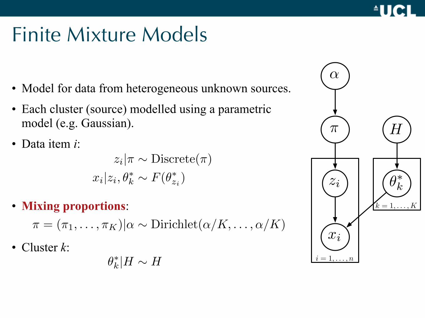
• Dirichlet distribution on the K-dimensional probability simplex { π | Σk πk = 1 }:
• with .
• Standard distribution on probability vectors, due to conjugacy with multinomial.
Γ(a) =�∞0 xa−1exdx zi
π
α
H
i = 1, . . . , n
xi
θ∗kk = 1, . . . ,K
P (π|α) = Γ(α)�k Γ(α/K)
K�
k=1
πα/K−1k
Dirichlet Distribution(1, 1, 1) (2, 2, 2)
(2, 2, 5)
(5, 5, 5)
(2, 5, 5) (0.7, 0.7, 0.7)
P (π|α) =Γ(
�k αk)�
k Γ(αk)
K�
k=1
παk−1k
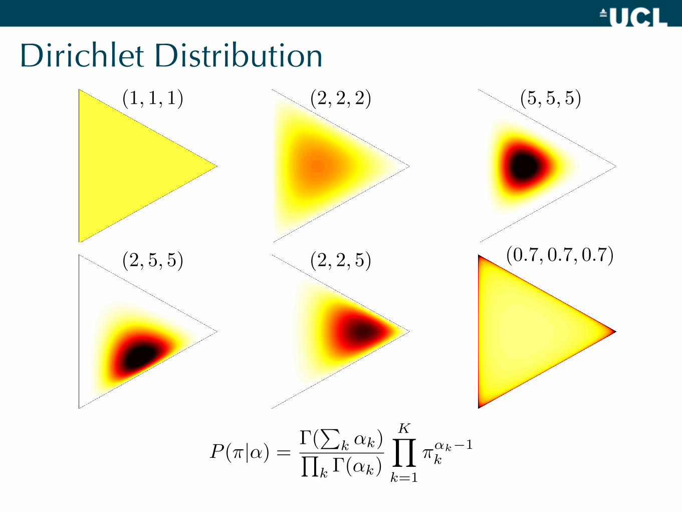
Dirichlet-Multinomial Conjugacy
• Joint distribution over zi and π:
• where nc = #{ zi = c }.
• Posterior distribution:
• Marginal distribution:
P (π|α)×n�
i=1
P (zi|π) =Γ(α)
�Kk=1 Γ(α/K)
K�
k=1
πα/K−1k ×
K�
k=1
πnkk
P (π|z,α) = Γ(n+ α)�K
k=1 Γ(nk + α/K)
K�
k=1
πnk+α/K−1k
P (z|α) = Γ(α)�K
k=1 Γ(α/K)
�Kk=1 Γ(nk + α/K)
Γ(n+ α)
Gibbs Sampling
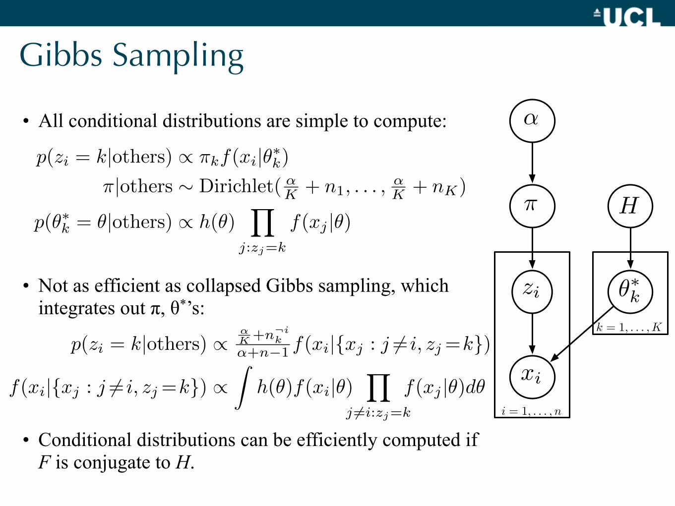
• All conditional distributions are simple to compute:
• Not as efficient as collapsed Gibbs sampling, which integrates out π, θ*’s:
• Conditional distributions can be efficiently computed if F is conjugate to H.
zi
π
α
H
i = 1, . . . , n
xi
θ∗kk = 1, . . . ,K
p(zi = k|others) ∝αK +n¬i
k
α+n−1 f(xi|{xj : j �= i, zj=k})
f(xi|{xj : j �= i, zj=k}) ∝�
h(θ)f(xi|θ)�
j �=i:zj=k
f(xj |θ)dθ
p(zi = k|others) ∝ πkf(xi|θ∗k)π|others ∼ Dirichlet( α
K + n1, . . . ,αK + nK)
p(θ∗k = θ|others) ∝ h(θ)�
j:zj=k
f(xj |θ)

Infinite Limit of Collapsed Gibbs Sampler
• We will take K → ∞.
• Imagine a very large value of K.
• There are at most n < K occupied clusters, so most components are empty. We can lump these empty components together:
zi
π
α
H
i = 1, . . . , n
xi
θ∗kk = 1, . . . ,K
p(zi = k|others) =n¬ik + α
K
n− 1 + αf(xi|{xj : j �= i, zj=k})
p(zi = kempty|others) =αK−K∗
K
n− 1 + αf(xi|{})
[Neal 2000, Rasmussen 2000, Ishwaran & Zarepour 2002]

Infinite Limit
• The actual infinite limit of the finite mixture model does not make sense:
• any particular cluster will get a mixing proportion of 0.
• Better ways of making this infinite limit precise:
• Chinese restaurant process.
• Stick-breaking construction.
• Both are different views of the Dirichlet process (DP).
• DPs can be thought of as infinite dimensional Dirichlet distributions.
• The K → ∞ Gibbs sampler is for DP mixture models.

Ferguson’s Definition of theDirichlet Process
Ferguson’s Definition of Dirichlet Processes
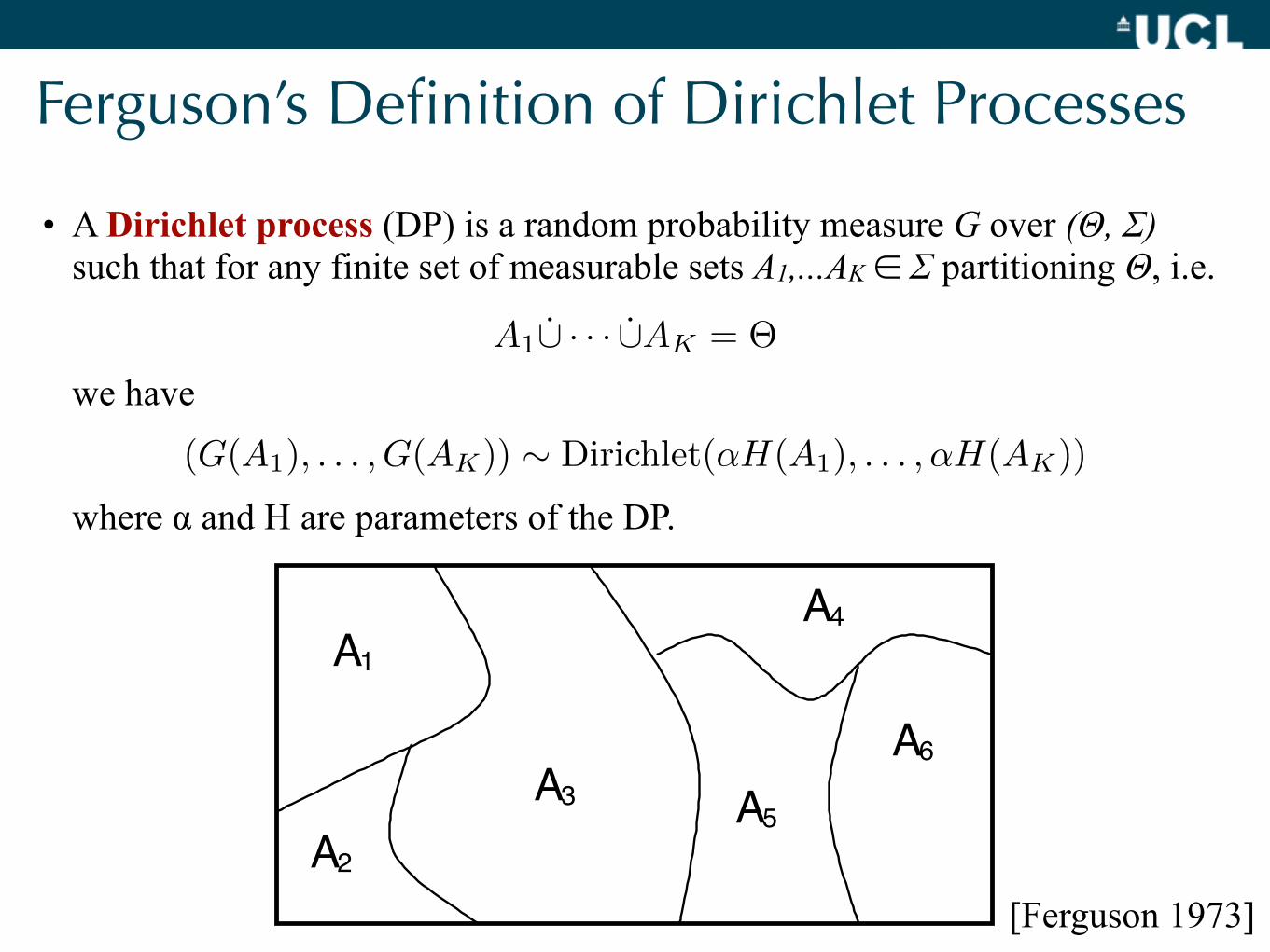
• A Dirichlet process (DP) is a random probability measure G over (Θ, Σ) such that for any finite set of measurable sets A1,...AK ∈ Σ partitioning Θ, i.e.
• we have
• where α and H are parameters of the DP.
A1∪̇ · · · ∪̇AK = Θ
(G(A1), . . . , G(AK)) ∼ Dirichlet(αH(A1), . . . ,αH(AK))
6
A
A1
A AA
A
2
3
4
5
[Ferguson 1973]
Parameters of the Dirichlet Process
• α is called the strength, mass or concentration parameter.
• H is called the base distribution.
• Mean and variance:
• where A is a measurable subset of Θ.
• H is the mean of G, and α is an inverse variance.
E[G(A)] = H(A)
V[G(A)] =H(A)(1−H(A))
α+ 1
Posterior Dirichlet Process
• Suppose
• We can define random variables that are G distributed:
• The usual Dirichlet-multinomial conjugacy carries over to the DP as well:
G ∼ DP(α, H)
θi|G ∼ G for i = 1, . . . , n
G|θ1, . . . , θn ∼ DP(α+ n,αH+
�ni=1 δθi
α+n)

Pólya Urn Scheme
• Marginalizing out G, we get:
• This is called the Pólya, Hoppe or Blackwell-MacQueen urn scheme.
• Start with an urn with α balls of a special colour.
• Pick a ball randomly from urn:
• If it is a special colour, make a new ball with colour sampled from H, note the colour, and return both balls to urn.
• If not, note its colour and return two balls of that colour to urn.
G ∼ DP(α, H)
θi|G ∼ G for i = 1, 2, . . .
θn+1|θ1, . . . , θn ∼ αH+�n
i=1 δθiα+n
[Blackwell & MacQueen 1973, Hoppe 1984]

Clustering Property
• The n variables θ1,θ2,...,θn can take on K ≤ n distinct values.
• Let the distinct values be θ1*,...,θK*. This defines a partition of {1,...,n} such that i is in cluster k if and only if θi = θk*.
• The induced distribution over partitions is the Chinese restaurant process.
G ∼ DP(α, H)
θi|G ∼ G for i = 1, 2, . . .
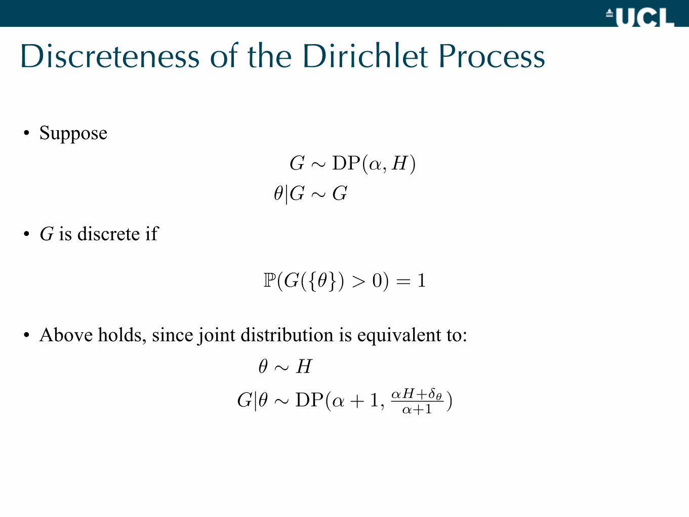
Discreteness of the Dirichlet Process
• Suppose
• G is discrete if
• Above holds, since joint distribution is equivalent to:
G ∼ DP(α, H)
θ|G ∼ G
P(G({θ}) > 0) = 1
θ ∼ H
G|θ ∼ DP(α+ 1, αH+δθα+1 )

A draw from a Dirichlet Process
0 0.1 0.2 0.3 0.4 0.5 0.6 0.7 0.8 0.9 10
5000
10000
15000
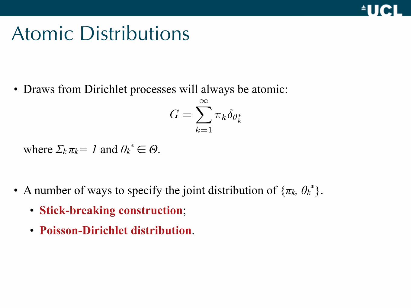
Atomic Distributions
• Draws from Dirichlet processes will always be atomic:
• where Σk πk = 1 and θk* ∈ Θ.
• A number of ways to specify the joint distribution of {πk, θk*}.
• Stick-breaking construction;
• Poisson-Dirichlet distribution.
G =∞�
k=1
πkδθ∗k

Random Partitions
[Aldous 1985, Pitman 2006]

Partitions
• A partition ϱ of a set S is:
• A disjoint family of non-empty subsets of S whose union in S.
• S = {Alice, Bob, Charles, David, Emma, Florence}.
• ϱ = { {Alice, David}, {Bob, Charles, Emma}, {Florence} }.
• Denote the set of all partitions of S as PS.
• Random partitions are random variables taking values in PS.
• We will work with partitions of S = [n] = {1,2,...n}.
AliceDavid
BobCharlesEmma
Florence

Chinese Restaurant Process
• Each customer comes into restaurant and sits at a table:
• Customers correspond to elements of S, and tables to clusters in ϱ.
• Rich-gets-richer: large clusters more likely to attract more customers.
• Multiplying conditional probabilities together, the overall probability of ϱ, called the exchangeable partition probability function (EPPF), is:
136
27
458
9
P (�|α) = α|�|Γ(α)
Γ(n+ α)
�
c∈�
Γ(|c|)
[Aldous 1985, Pitman 2006]
p(sit at table c) =nc
α+�
c∈� ncp(sit at new table) =
α
α+�
c∈� nc

Number of Clusters• The prior mean and variance of K are:
ψ(α) = ∂∂α logΓ(α)
0 2000 4000 6000 8000 100000
50
100
150
200
customer
table
!=30, d=0
0 20 40 60 80 1000
0.02
0.04
0.06
0.08
0.1
0.12alpha = 10
E[|ρ||α, n] = α(ψ(α+ n)− ψ(α)) ≈ α log�1 + n
α
�
V[|ρ||α, n] = α(ψ(α+ n)− ψ(α)) + α2(ψ�(α+ n)− ψ�(α)) ≈ α log�1 + n
α
�
Model-based Clustering with Chinese Restaurant Process

Partitions in Model-based Clustering
• Partitions are the natural latent objects of inference in clustering.
• Given a dataset S, partition it into clusters of similar items.
• Cluster c ∈ ϱ described by a model
parameterized by θc*.
• Bayesian approach: introduce prior over ϱ and θc*; compute posterior over both.
F (θ∗c )
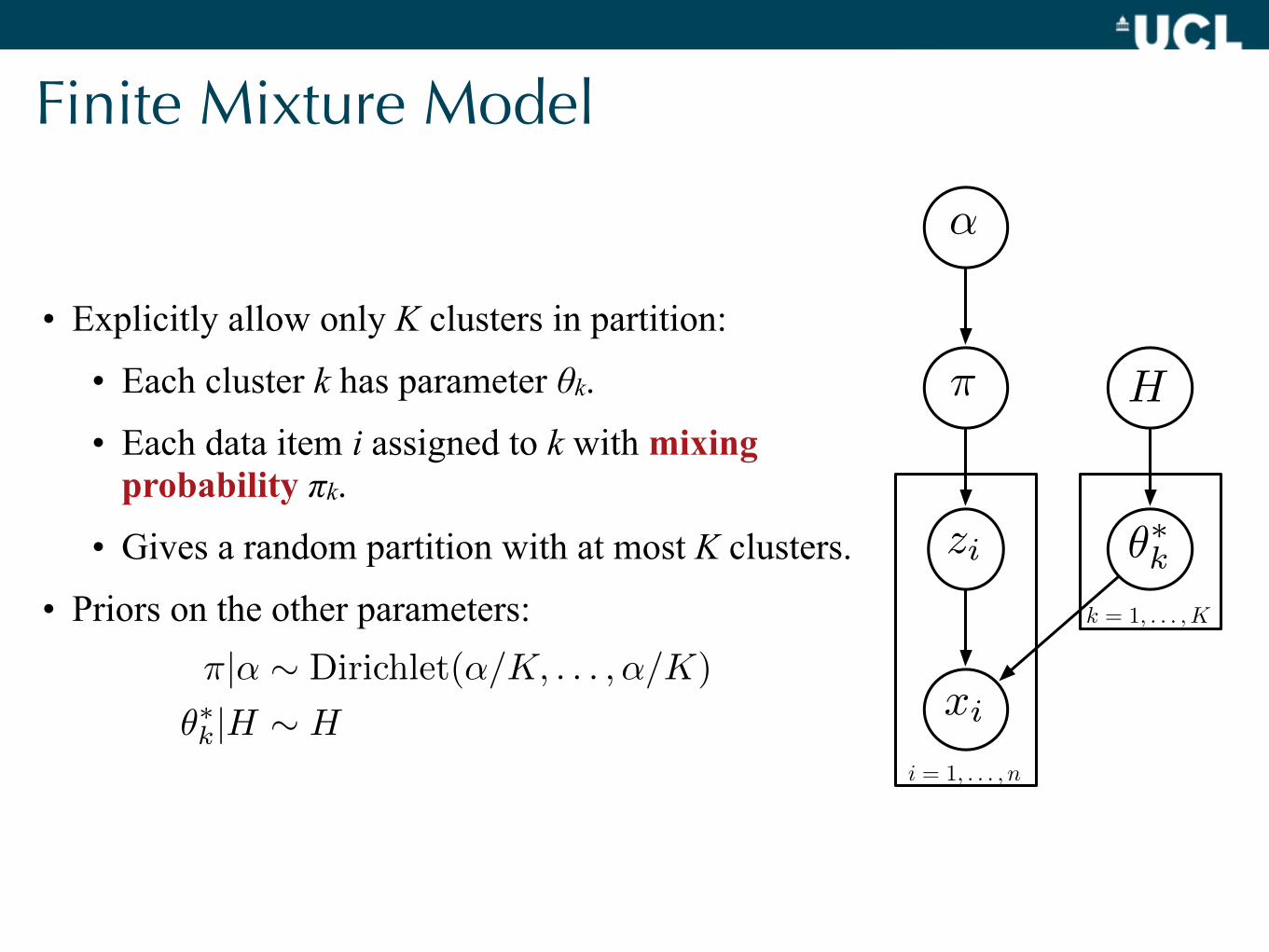
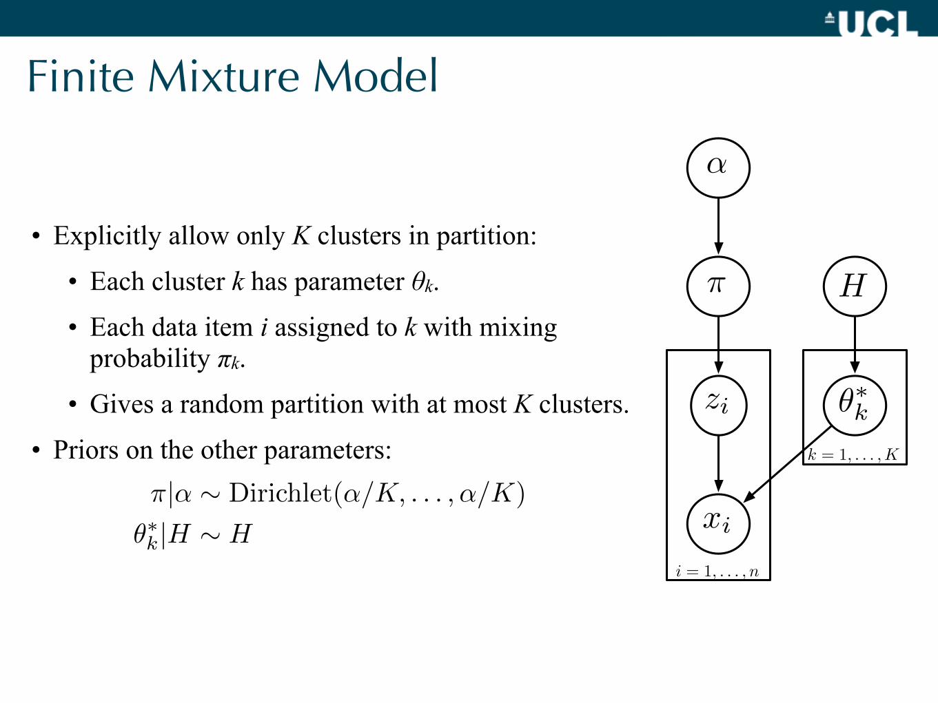
Finite Mixture Model
• Explicitly allow only K clusters in partition:
• Each cluster k has parameter θk.
• Each data item i assigned to k with mixing probability πk.
• Gives a random partition with at most K clusters.
• Priors on the other parameters:
•
zi
π
α
H
i = 1, . . . , n
xi
θ∗kk = 1, . . . ,K
π|α ∼ Dirichlet(α/K, . . . ,α/K)
θ∗k|H ∼ H
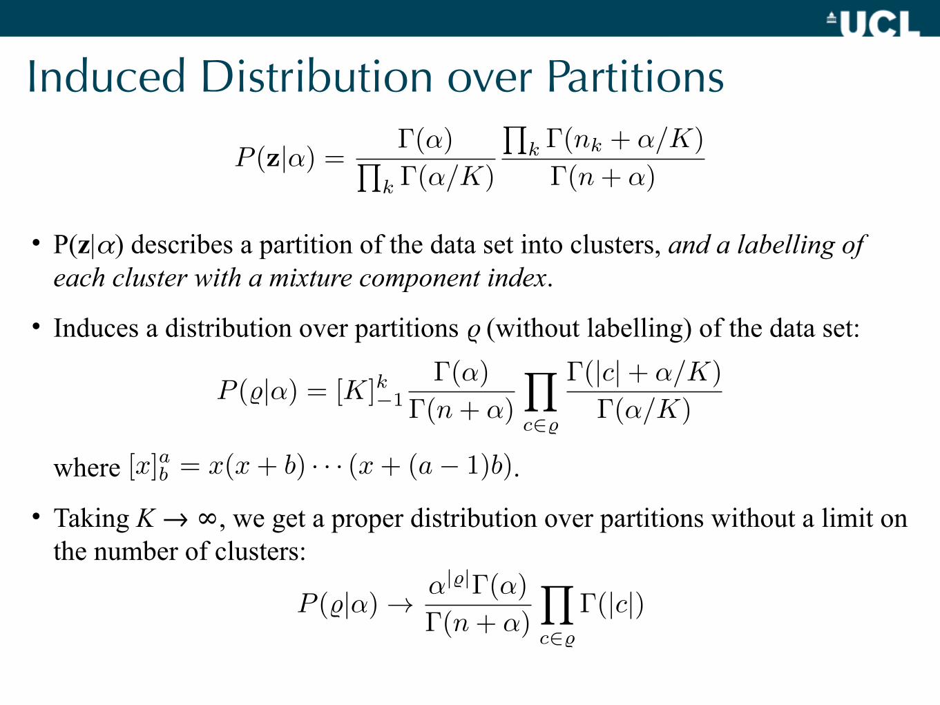
Induced Distribution over Partitions
• P(z|α) describes a partition of the data set into clusters, and a labelling of each cluster with a mixture component index.
• Induces a distribution over partitions ϱ (without labelling) of the data set:
• where .
• Taking K → ∞, we get a proper distribution over partitions without a limit on the number of clusters:
P (�|α) = [K]k−1Γ(α)
Γ(n+ α)
�
c∈�
Γ(|c|+ α/K)
Γ(α/K)
[x]ab = x(x+ b) · · · (x+ (a− 1)b)
P (�|α) → α|�|Γ(α)
Γ(n+ α)
�
c∈�
Γ(|c|)
P (z|α) = Γ(α)�k Γ(α/K)
�k Γ(nk + α/K)
Γ(n+ α)

Chinese Restaurant Process
• An important representation of the Dirichlet process
• An important object of study in its own right.
• Predates the Dirichlet process and originated in genetics (related to Ewen’s sampling formula there).
• Large number of MCMC samplers using CRP representation.
• Random partitions are useful concepts for clustering problems in machine learning
• CRP mixture models for nonparametric model-based clustering.
• hierarchical clustering using concepts of fragmentations and coagulations.
• clustering nodes in graphs, e.g. for community discovery in social nets.
• Other combinatorial structures can be built from partitions.
Random Probability Measures

A draw from a Dirichlet Process
0 0.1 0.2 0.3 0.4 0.5 0.6 0.7 0.8 0.9 10
5000
10000
15000

Atomic Distributions
• Draws from Dirichlet processes will always be atomic:
• where Σk πk = 1 and θk* ∈ Θ.
• A number of ways to specify the joint distribution of {πk, θk*}.
• Stick-breaking construction;
• Poisson-Dirichlet distribution.
G =∞�
k=1
πkδθ∗k
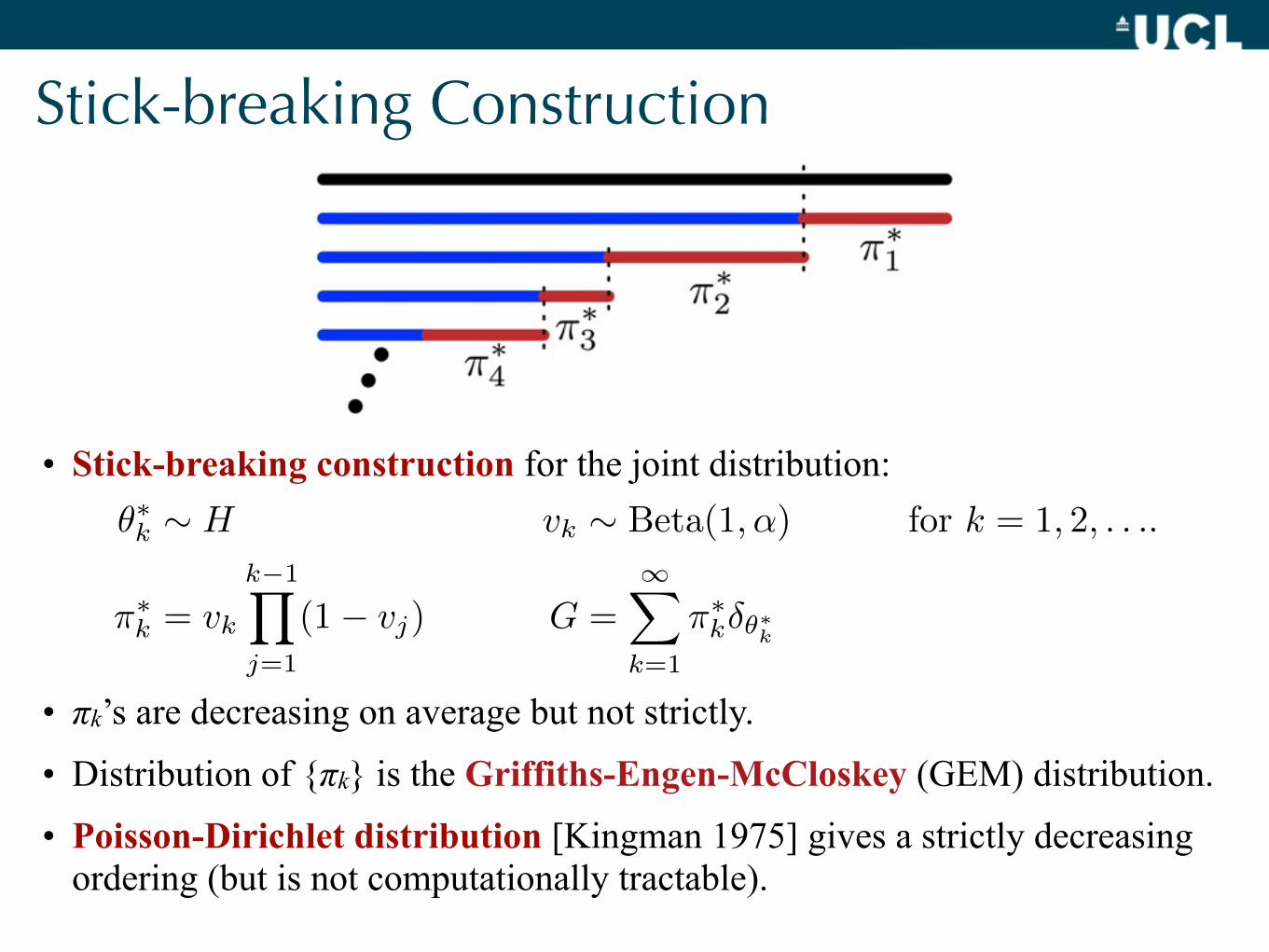
Stick-breaking Construction
• Stick-breaking construction for the joint distribution:
• πk’s are decreasing on average but not strictly.
• Distribution of {πk} is the Griffiths-Engen-McCloskey (GEM) distribution.
• Poisson-Dirichlet distribution [Kingman 1975] gives a strictly decreasing ordering (but is not computationally tractable).
θ∗k ∼ H vk ∼ Beta(1,α) for k = 1, 2, . . ..
π∗k = vk
k−1�
j=1
(1− vj) G =∞�
k=1
π∗kδθ∗
k
Finite Mixture Model
• Explicitly allow only K clusters in partition:
• Each cluster k has parameter θk.
• Each data item i assigned to k with mixing probability πk.
• Gives a random partition with at most K clusters.
• Priors on the other parameters:
•
zi
π
α
H
i = 1, . . . , n
xi
θ∗kk = 1, . . . ,K
π|α ∼ Dirichlet(α/K, . . . ,α/K)
θ∗k|H ∼ H

Size-biased Permutation
• Reordering clusters do not change the marginal distribution on partitions or data items.
• By strictly decreasing πk: Poisson-Dirichlet distribution.
• Reorder stochastically as follows gives stick-breaking construction:
• Pick cluster k to be first cluster with probability πk .
• Remove cluster k and renormalize rest of { πk : j ≠ k }; repeat.
• Stochastic reordering is called a size-biased permutation.
• After reordering, taking K → ∞ gives the corresponding DP representations.

Stick-breaking Construction
• Easy to generalize stick-breaking construction:
• to other random measures;
• to random measures that depend on covariates or vary spatially.
• Easy to work with different algorithms:
• MCMC samplers;
• variational inference;
• parallelized algorithms.
[Ishwaran & James 2001, Dunson 2010 and many others]
DP Mixture Model: Representations and Inference

DP Mixture Model
• A DP mixture model:
• Different representations:
• θ1,θ2,...,θn are clustered according to Pólya urn scheme, with induced partition given by a CRP.
• G is atomic with weights and atoms described by stick-breaking construction.
[Neal 2000, Rasmussen 2000, Ishwaran & Zarepour 2002]
G|α, H ∼ DP(α, H)
θi|G ∼ G
xi|θi ∼ F (θi)

CRP Representation
• Representing the partition structure explicitly with a CRP:
• Makes explicit that this is a clustering model.
• Using a CRP prior for ϱ obviates need to limit number of clusters as in finite mixture models.
[Neal 2000, Rasmussen 2000, Ishwaran & Zarepour 2002]
ρ|α ∼ CRP([n],α)
θ∗c |H ∼ H for c ∈ ρ
xi|θ∗c ∼ F (θ∗c ) for c � i

Marginal Sampler• “Marginal” MCMC sampler.
• Marginalize out G, and Gibbs sample partition.
• Conditional probability of cluster of data item i:
• A variety of methods to deal with new clusters.
• Difficulty lies in dealing with new clusters, especially when prior h is not conjugate to f.
[Neal 2000]
ρ|α ∼ CRP([n],α)
θ∗c |H ∼ H for c ∈ ρ
xi|θ∗c ∼ F (θ∗c ) for c � i
P (ρi|ρ\i,x,θ) =P (ρi|ρ\i)P (xi|ρi,x\i,θ)
P (ρi|ρ\i) =�
|c|n−1+α if ρi = c ∈ ρ\i
αn−1+α if ρi = new
P (xi|ρi,x\i,θ) =
�f(xi|θρi) if ρi = c ∈ ρ\i�f(xi|θ)h(θ)dθ if ρi = new

Induced Prior on the Number of Clusters• The prior expectation and variance of |ϱ| are:E[|ρ||α, n] = α(ψ(α+ n)− ψ(α)) ≈ α log
�1 + n
α
�
V[|ρ||α, n] = α(ψ(α+ n)− ψ(α)) + α2(ψ�(α+ n)− ψ�(α)) ≈ α log�1 + n
α
�
0 20 40 60 80 1000
0.05
0.1
0.15
0.2
0.25alpha = 1
0 20 40 60 80 1000
0.02
0.04
0.06
0.08
0.1
0.12alpha = 10
0 20 40 60 80 1000
0.02
0.04
0.06
0.08
0.1alpha = 100

Marginal Gibbs Sampler Pseudocode• Initialize: randomly assign each data item to some cluster.• K := the number of clusters used.• For each cluster k = 1...K:
• Compute sufficient statistics sk := Σ { s(xi) : zi = k }.• Compute cluster sizes nk := # { i : zi = k }.
• Iterate until convergence:• For each data item i = 1...n:
• Let k := zi be the current cluster data item is assigned to.• Remove data item: sk −= s(xi), nk −= 1.• If nk = 0 then remove cluster k (K −= 1 and relabel rest of clusters). • Compute conditional probabilities p(zi=c|others)
for c = 1...K, kempty := K+1.• Sample new cluster for data item from conditional probabilities.• If c = kempty then create new cluster: K+=1, sc := 0, nc = 0. • Add data item: zi := c, sc += s(xi), nc += 1.
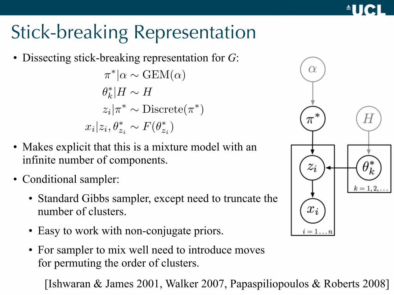
Stick-breaking Representation• Dissecting stick-breaking representation for G:
• Makes explicit that this is a mixture model with an infinite number of components.
• Conditional sampler:
• Standard Gibbs sampler, except need to truncate the number of clusters.
• Easy to work with non-conjugate priors.
• For sampler to mix well need to introduce moves for permuting the order of clusters.
π∗|α ∼ GEM(α)
θ∗k|H ∼ H
zi|π∗ ∼ Discrete(π∗)
xi|zi, θ∗zi ∼ F (θ∗zi)
[Ishwaran & James 2001, Walker 2007, Papaspiliopoulos & Roberts 2008]
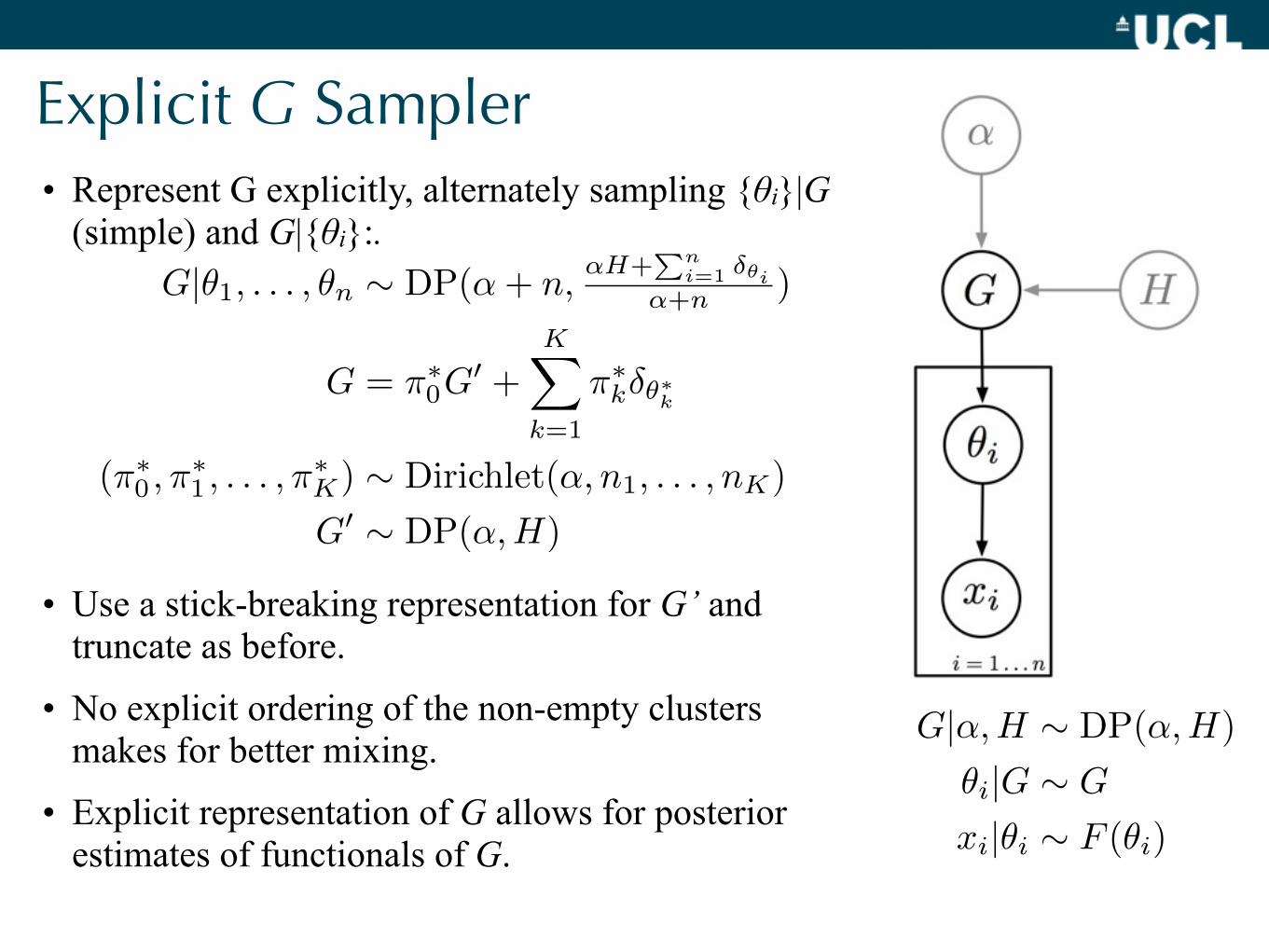
Explicit G Sampler• Represent G explicitly, alternately sampling {θi}|G
(simple) and G|{θi}:.
• Use a stick-breaking representation for G’ and truncate as before.
• No explicit ordering of the non-empty clusters makes for better mixing.
• Explicit representation of G allows for posterior estimates of functionals of G.
G|α, H ∼ DP(α, H)
θi|G ∼ G
xi|θi ∼ F (θi)
G|θ1, . . . , θn ∼ DP(α+ n,αH+
�ni=1 δθi
α+n)
G = π∗0G
� +K�
k=1
π∗kδθ∗
k
(π∗0 ,π
∗1 , . . . ,π
∗K) ∼ Dirichlet(α, n1, . . . , nK)
G� ∼ DP(α, H)
Other Inference Algorithms
• Split-merge algorithms [Jain & Neal 2004].
• Close in spirit to reversible-jump MCMC methods [Green & richardson 2001].
• Sequential Monte Carlo methods [Liu 1996, Ishwaran & James 2003, Fearnhead 2004, Mansingkha et al 2007].
• Variational algorithms [Blei & Jordan 2006, Kurihara et al 2007, Teh et al 2008].
• Expectation propagation [Minka & Ghahramani 2003, Tarlow et al 2008].


![[DRAFT:PleaseDoNotDistribute]teh/outbox/jordan-teh.pdfA Gentle Introduction to the Dirichlet Process, the Beta Process and Bayesian Nonparametrics [DRAFT:PleaseDoNotDistribute] MichaelI.Jordan&YeeWhyeTeh](https://img.dokumen.tips/doc/110x75/5f909ad38e03840c023efe81/draftpleasedonotdistribute-tehoutboxjordan-tehpdf-a-gentle-introduction-to.jpg)