Bayesian Methods for Measuring Operational Risks regulators and the financial services industry in their quest to construct meaningful measures for operational risks

ICBI Technical Risk Management Reports

© Carol Alexander 1

Bayesian Methods for Measuring Operational Risks

Carol Alexander

ISMA Centre, Reading University, UK1

This paper shows how Bayesian methods may be applied to measure a variety of operational risks, including those that are difficult to quantify. The advantage of Bayesian estimation over classical estimation for operational risk is that subjective prior beliefs play an important role. Bayesian networks improve transparency for efficient risk management, being based on causal

flows in an operational process. They also lend themselves to back testing, and to scenario analysis to identify maximum loss. Many examples in this paper include human risk, settlement

risk and the Bayesian measurement of operational risk scores.

Many articles, surveys and books begin with long discussions of the various definitions of operational risks. For example see Hoffman (1998) and the BBA/ISDA/RMA survey (2000). It is a difficult and important issue, but there is no need to regurgitate yet another account of the problems here. Instead, the introduction to this article focuses on some of the fundamental issues for regulators and the financial services industry in their quest to construct meaningful measures for operational risks. The measurement of any financial risk requires calculation of a loss distribution. From this distribution the important quantities to be measured are the expected loss and the 'tail' loss. In market and credit risks the expected loss is taken into account in the mark to market, in the pricing or provisioning for the portfolio and the tail loss is used to estimate risk capital reserves. Similarly for operational risks, both expected loss and tail loss need to be measured, and the relative importance of each measure will depend on the type of operational risk. Operational risks are categorized according their impact on the ability of the firm to function, and the frequency with which they arise.2 High frequency low impact operational risks such as settlement risk have an expected loss of the same order of magnitude as the standard deviation of loss. So the tail loss for this type of operational risk has a relatively low impact on the ability of the firm to function, but the expected loss has a relatively large impact on daily profit and loss. On the other hand, low frequency high impact operational risks such as fraud have a small expected loss but a tail loss that could have an enormous influence on the operation of the firm.

Thus regulators and industry players alike should be concentrating on taking account of the expected loss for high frequency low impact operational risks and the tail loss for low frequency high impact operational risks. It is not yet clear whether regulators will ask for additional capital

1 Many thanks to Telia Wiesman of Randloph Ivy Women's College for enthusiastic research assistance. 2 Operational risks include many different types of risk, from the simple 'operations' risks of transactions processing, unauthorized activities, and system risks to other types of risk that are not included in market or credit risk: human risk, legal risk, information risk, and reputational risk.



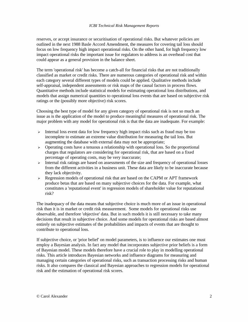
reserves, or accept insurance or securitisation of operational risks. But whatever policies are outlined in the next 1988 Basle Accord Amendment, the measures for covering tail loss should focus on low frequency high impact operational risks. On the other hand, for high frequency low impact operational risks the important issue for regulators to address is an overhead cost that could appear as a general provision in the balance sheet.

The term 'operational risk' has become a catch-all for financial risks that are not traditionally classified as market or credit risks. There are numerous categories of operational risk and within each category several different types of models could be applied. Qualitative methods include self-appraisal, independent assessments or risk maps of the causal factors in process flows. Quantitative methods include statistical models for estimating operational loss distributions, and models that assign numerical quantities to operational loss events that are based on subjective risk ratings or the (possibly more objective) risk scores. Choosing the best type of model for any given category of operational risk is not so much an issue as is the application of the model to produce meaningful measures of operational risk. The major problem with any model for operational risk is that the data are inadequate. For example: Ø Internal loss event data for low frequency high impact risks such as fraud may be too

incomplete to estimate an extreme value distribution for measuring the tail loss. But augmenting the database with external data may not be appropriate;

Ø Operating costs have a tenuous a relationship with operational loss. So the proportional charges that regulators are considering for operational risk, that are based on a fixed percentage of operating costs, may be very inaccurate;

Ø Internal risk ratings are based on assessments of the size and frequency of operational losses from the different activities in a business unit. These data are likely to be inaccurate because they lack objectivity.

Ø Regression models of operational risk that are based on the CAPM or APT framework produce betas that are based on many subjective choices for the data. For example, what constitutes a 'reputational event' in regression models of shareholder value for reputational risk?

The inadequacy of the data means that subjective choice is much more of an issue in operational risk than it is in market or credit risk measurement. Some models for operational risks use observable, and therefore 'objective' data. But in such models it is still necessary to take many decisions that result in subjective choice. And some models for operational risks are based almost entirely on subjective estimates of the probabilities and impacts of events that are thought to contribute to operational loss. If subjective choice, or 'prior belief' on model parameters, is to influence our estimates one must employ a Bayesian analysis. In fact any model that incorporates subjective prior beliefs is a form of Bayesian model. These models therefore have a crucial role to play in modelling operational risks. This article introduces Bayesian networks and influence diagrams for measuring and managing certain categories of operational risks, such as transaction processing risks and human risks. It also compares the classical and Bayesian approaches to regression models for operational risk and the estimation of operational risk scores.



Example 1: Human Risk Operational losses that are incurred through inadequate staffing for required activities are commonly termed 'human risks'. These may be due to due to lack of training, poor recruitment processes, inadequate pay, poor working culture, loss of key employees, bad management, and so on. Some operational risk score data on human risks might be available, such as expenditure on employee training, staff turnover rates, numbers of complaints, and so on. But human risk remains one of the most difficult operational risks to quantify because the only information available on many of the important causal factors will be subjective beliefs. A simplified example illustrates how Bayes rule may be applied to quantify a human risk. Suppose you are in charge of client services, and your team in the UK has not been very reliable. In fact your prior belief is that one fifth of the time they provide unsatisfactory service. If they are operating efficiently, customer complaints data indicates that about 80% of clients would be satisfied. This could be translated into 'the probability of losing a client when the team operates well is 0.2'. But your past experience shows that the number of customer complaints rises rapidly when a team operates ineffectually, and when this occurs the probability of losing a client rises from 0.2 to 0.65. Now suppose that a client of the UK team has been lost. In the light of this further information, what is your revised probability that the UK team provided unsatisfactory service? To answer this question, let X be the event ‘unsatisfactory service’ and Y be the event ‘lose the client’. Your prior belief is that prob(X) = 0.2 and so

prob(Y) = prob(YX) prob(X) + prob (Ynot X) prob (not X) = 0.65 * 0.2 + 0.2 * 0.8 = 0.29.

Now Bayes’ rule gives the posterior probability of unsatisfactory service, given that a client has been lost as:

prob(XY) = prob(YX) prob(X)/prob(Y) = 0.65 * 0.2 / 0.29 = 0.448

Thus your belief that the UK team does not provide good service one-fifth of the time has been revised in the light of the information that a client has been lost. You now believe that they provide inadequate service almost half the time!

Bayes' Rule The Reverend Thomas Bayes (1702-1761) viewed the process of statistical estimation as one of continuously revising and refining our subjective beliefs about the state of the world as more data become available. His "Essay Towards Solving a Problem in the Doctrine of Chances", published posthumously in 1763, introduced the method for updating beliefs that is now referred to as Bayes' rule. The cornerstone of Bayesian methods is the theorem of conditional probability of events X and Y:



prob(X and Y) = prob(XY) prob(Y) = prob(YX) prob(X) This can be re-written in a form that is known as Bayes’ rule, which shows how prior information about Y may be used to revise the probability of X:

prob(XY) = prob(YX) prob(X) / prob(Y) (1)

The Value of Information Classical statistical inference on an operational risk involves estimating the likelihood of the data to give a loss distribution, given the current values of the parameters. In classical statistics the model parameters are assumed to be fixed, although unknown at any point in time. But in the Bayesian approach this problem is turned around, and instead of asking 'what is the probability of a loss, given the model parameters' the question becomes 'what is the probability of the parameters, given the data'? When Bayes' rule is applied to distributions about model parameters it becomes:

prob(parametersdata) = prob(dataparameters)*prob(parameters) / prob(data) The unconditional probability of the data 'prob(data)' only serves as a scaling constant, and the generic form of Bayes' rule is usually written:

prob(parameters data) ∝ prob(dataparameters)*prob(parameters) (2) Prior beliefs about the parameters are given by the prior density 'prob(parameters)' and the likelihood of the sample data 'prob(dataparameters)' is called the sample likelihood. The product of these two densities defines the posterior density 'prob(parameters data)', that incorporates both prior beliefs and sample information into a revised and updated view of the model parameters, as depicted in figure 1.

Figure 1: The posterior density is a product of the prior density and the sample likelihood

Prior

Likelihood Posterior

Parameter



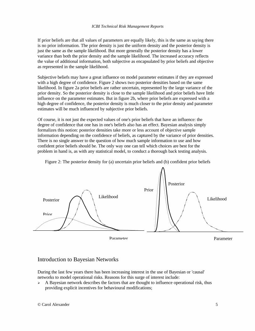
If prior beliefs are that all values of parameters are equally likely, this is the same as saying there is no prior information. The prior density is just the uniform density and the posterior density is just the same as the sample likelihood. But more generally the posterior density has a lower variance than both the prior density and the sample likelihood. The increased accuracy reflects the value of additional information, both subjective as encapsulated by prior beliefs and objective as represented in the sample likelihood. Subjective beliefs may have a great influence on model parameter estimates if they are expressed with a high degree of confidence. Figure 2 shows two posterior densities based on the same likelihood. In figure 2a prior beliefs are rather uncertain, represented by the large variance of the prior density. So the posterior density is close to the sample likelihood and prior beliefs have little influence on the parameter estimates. But in figure 2b, where prior beliefs are expressed with a high degree of confidence, the posterior density is much closer to the prior density and parameter estimates will be much influenced by subjective prior beliefs. Of course, it is not just the expected values of one's prior beliefs that have an influence: the degree of confidence that one has in one's beliefs also has an effect. Bayesian analysis simply formalizes this notion: posterior densities take more or less account of objective sample information depending on the confidence of beliefs, as captured by the variance of prior densities. There is no single answer to the question of how much sample information to use and how confident prior beliefs should be. The only way one can tell which choices are best for the problem in hand is, as with any statistical model, to conduct a thorough back testing analysis.

Figure 2: The posterior density for (a) uncertain prior beliefs and (b) confident prior beliefs

Introduction to Bayesian Networks During the last few years there has been increasing interest in the use of Bayesian or 'causal' networks to model operational risks. Reasons for this surge of interest include: Ø A Bayesian network describes the factors that are thought to influence operational risk, thus

providing explicit incentives for behavioural modifications;

Prior

Likelihood Posterior

Parameter

Prior Likelihood

Posterior

Parameter



Ø Bayesian networks have the ability to perform scenario analysis to measure maximum operational loss, and to integrate operational risk with market and credit risk;

Ø The variety of operational risks to which Bayesian networks can be applied. Over and above the categories where available data enable the modelling of operational risk with standard statistical models, Bayesian networks have applications to areas where data are difficult to quantify, such as human risks;

Ø Augmenting a Bayesian network with decision nodes and utilities improves transparency for management decisions.

The basic structure of a Bayesian network is a directed acyclic graph where nodes represent random variables and links represent causal influence. There is no unique Bayesian network to represent any situation, unless it is extremely simple. Rather, a Bayesian network should be regarded as the analyst's view of process flows, and how the various causal factors interact. In general, many different Bayesian networks could be used to depict the same process. A simple Bayesian network that models the client services team of example 1 is shown in figure 3. The nodes 'Team', 'Market' and 'Client' represent random variables each with two possible outcomes, and the probability distribution on the outcomes is shown on the right of the figure. It is only necessary to specify the probability distribution of the two parent nodes (Team and Market) and the conditional probabilities for the Contract . The four conditional probabilities 'prob(winmarket = good and team = not satisfactory)' and so on, are shown below the Contract node. The network then calculates prob(win) = 71% and prob(lose) = 29%, using Bayes rule. The Bayesian network may be used for scenario analyses. For example, if the contract is lost, what is the revised probability of the team being unsatisfactory? The bottom right box in figure 3 shows that the posterior probability that the team is unsatisfactory given that the contract has been lost is 44.83%, as already calculated in example 1.

Figure 3: A simple Bayesian network for the client services problem



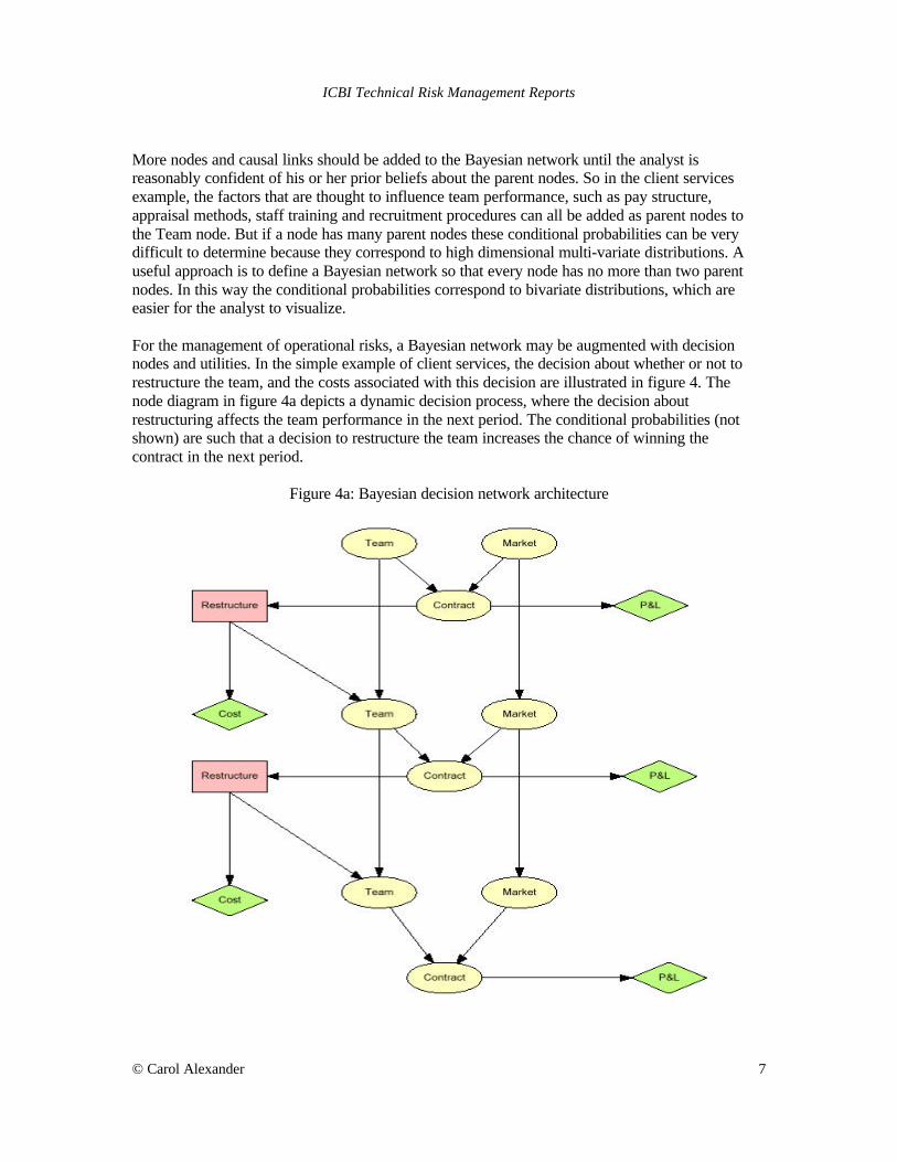
More nodes and causal links should be added to the Bayesian network until the analyst is reasonably confident of his or her prior beliefs about the parent nodes. So in the client services example, the factors that are thought to influence team performance, such as pay structure, appraisal methods, staff training and recruitment procedures can all be added as parent nodes to the Team node. But if a node has many parent nodes these conditional probabilities can be very difficult to determine because they correspond to high dimensional multi-variate distributions. A useful approach is to define a Bayesian network so that every node has no more than two parent nodes. In this way the conditional probabilities correspond to bivariate distributions, which are easier for the analyst to visualize. For the management of operational risks, a Bayesian network may be augmented with decision nodes and utilities. In the simple example of client services, the decision about whether or not to restructure the team, and the costs associated with this decision are illustrated in figure 4. The node diagram in figure 4a depicts a dynamic decision process, where the decision about restructuring affects the team performance in the next period. The conditional probabilities (not shown) are such that a decision to restructure the team increases the chance of winning the contract in the next period.

Figure 4a: Bayesian decision network architecture



In the initial state of the network, with the utilities and prior probabilities shown in the left column of figure 4b, there is a utility of 19.38 if the team is restructured at the end of the first period, but a utility of 20.33 if it is not restructured. So the optimal decision would be to leave the team is it is. However if the contract in the first period were lost (a scenario shown in the right column of figure 4b) the situation reverses, and it become more favorable to restructure the team. A similar scenario analysis shows that if the recommendation of the network is ignored and the team is not restructured, and if the contract in the second period is also lost, the utility from restructuring in the second period would be 1.79. The utility is 1.52 if the team were left unchanged, so again the network recommends a restructuring of the team.

Figure 4b: Bayesian decision network - probabilities and utilities



This example shows how a Bayesian network may be augmented with decision variables to focus on operational management decision processes. Just one of many possible scenarios has been illustrated, and to explore more possibilities the interested reader is encouraged to replicate this example, or to construct a decision network more relevant to their own needs, using a Bayesian network package.3

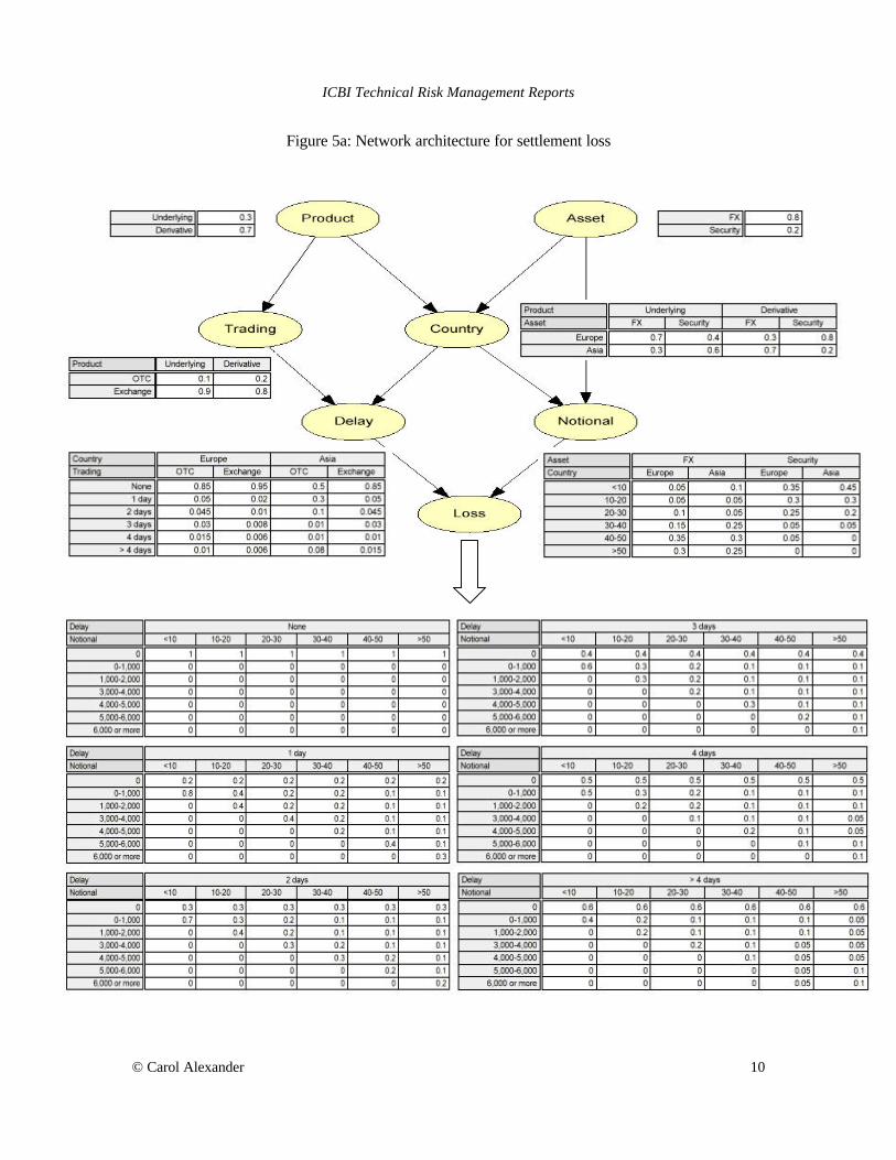
Application of Bayesian Networks to Operational Loss Distributions This section presents a Bayesian network model of the operational loss from settlement risk. This is the loss arising from interest foregone, fines imposed or borrowing costs as a result of a delay in settlement. It does not include the credit loss if the settlement delay is due to counterparty default, but it may include any legal or human costs incurred when settlement is delayed. Lack of space precludes an attempting a complete specification of the type of network that a bank might use for settlement loss in practice.4 The model is presented in a simplified form, but is sufficient to illustrate how Bayesian networks: Ø specify the causal factors that influence an operational loss distribution; Ø back test against historical loss event data to revise the network parameters; Ø employ scenario analysis to identify maximum operational loss. Figure 5 illustrates a Bayesian network that models a settlement loss distribution. Data from the trading book provide the probabilities for each node. For example the probabilities assigned to the 'Country' node show that 70% of spot FX trades are in European currencies, and 20% of derivative securities trades are in Asia. Similarly the 'Delay' node shows that only 50% of over-the-counter trades in Asia experienced no delay, 0.6% of exchange traded European assets experienced five or more days delay in settlement, and so on. And the 'Notional' node shows that 35% of European FX trades were in deals in the 40-50$m bracket, but just 5% of trades in European securities fall into this bracket.

There are many conditional probabilities in the 'Loss' node even in this simplified model. The loss is calculated as a function L(m,t) of the notional m and the number of days delay t. This function depends on many things, including the settlement process (delivery vs payment, escrow, straight-through, and so on), and whether legal and human costs are included in settlement loss. In the example the notional of a transaction is bucketed into 10$m brackets, and the loss distribution is given in round $000's. So for example the loss distribution in the initial state, shown in the left column in figure 5b, gives an expected loss of 274.4$ per transaction and a 99% tail loss of 4,763$ per transaction.

3 There are several software packages for Bayesian networks that are freely downloadable from the Internet. Microsoft provides a free package for personal research only that is Excel compatible at www.research.microsoft.com/research.dtg/msbn/default.htm and a list of free (and other) Bayesian network software is on http.cs.berkeley.edu/~murphyk/Bayes/bnsoft.html 4 Such a model has been developed by Algorithmics Inc. (see www.algorithmics.com).



Figure 5a: Network architecture for settlement loss



Obviously this picture of the settlements process is neither unique nor unique. For example the analyst might wish to categorize trades not just by country and asset type, but also according to whether the trades were in derivatives or the underlying. In that case the architecture of the network should be amended by adding a causal link from the 'Product' node to the 'Notional' node. Alternative architectures could have the 'Country' node as a root node, or other nodes could be added such as the settlement process or the method for order processing. And most nodes in this example have been simplified to have only two states, so 'Country' can only be Europe or Asia, 'Asset' can be only foreign exchange or security, and so on. But the generalization of the network to more states in any of these variables is straightforward and the simple node structure given here is clear enough to illustrate the main ideas. Which is the best of many possible specifications of a Bayesian network for settlement loss will depend on the results of back tests. A number of different network architectures for modelling settlement loss could be tested. For each, the initial probabilities5 should be based on the current trading book, and the result of the network in this initial state could then be compared with the current settlement loss experienced. A basis for back testing is to compare the actual settlement loss that is recorded with the predicted loss, using a chi-squared goodness-of-fit test. By performing back tests over suitable historic data, perhaps weekly during a one-year period, the best network design would be the one that gives the smallest chi-squared statistic. Bayesian networks lend themselves very easily to scenario analysis. The operational risk manager can ask the question 'what is the expected settlement loss from over-the-counter trading in Asian FX futures'? The right column in figure 5b illustrates this scenario: per transaction the expected loss is 1,069.5$ and the 99% tail loss is 5,679$. Similarly the manager might ask 'what is the expected settlement loss from an FX trade in the 40-50$m bracket'? By setting probabilities of 1 on FX in the 'Product' node and on 40-50$m in the 'Notional' node, the answer is quickly calculated as 400.5$m. The interested reader can verify this is by replicating the network with one of the packages mentioned in footnote 3. With answers to questions such as this, operational risk managers can identify the types of trades and operations where the settlement process is likely to present the greatest risk. Bayesian networks are not the only models that measure settlement loss, after all if historic data are available for back testing a network then they could be used to generate empirical settlement loss distributions. But they certainly improve transparency for operational risk management.

Bayesian Estimation Bayesians view an estimate b of a parameter β as an optimal choice, where the decision criterion is to minimize the expected loss. Expected loss is defined by a loss function some probability distribution over all possible outcomes, and in Bayesian estimation the probabilities are given by the posterior distribution. Standard loss functions are: Zero-one (L(β,b) = 0 if β = b and 1 otherwise); Absolute (L(β,b) = β - b); Quadratic (L(β,b) = (β - b)2). The Bayesian estimator

5 That is, the probabilities from the initial propagation of the network, before it is propagated again for scenario analysis.



will be the mode, median or mean of the posterior density according as the zero-one, absolute or quadratic loss function is used.

Figure 5b: Scenario analysis for settlement loss

Maximum likelihood estimation is regarded as the jewel in the crown of classical statistical inference because it gives consistent and asymptotically efficient estimators. But maximum likelihood estimation is but a crude form of Bayesian estimation. It corresponds to the Bayesian estimator with (a) a zero-one loss function (which is rather simplistic), so the Bayesian estimator is the mode of the posterior, and (b) no prior information, so that the posterior is the likelihood. You may think that by using a standard classical estimator of a proportion you are not actually employing any subjective choice, but this is not the case. In fact by choosing to use maximum likelihood estimation, your belief is that the proportion is very close to either zero or one!

Example 2 illustrates how these peculiar assumptions on model parameters are implicit in the simple maximum likelihood estimator of a proportion. If n occurrences are observed in a sample



size m, the maximum likelihood estimator is just n/m. To understand how the Bayesian estimators are derived, recall that a beta density

f(p) ∝ pa (1-p)b for 0 < p< 1 may be used to approximate more or less any distribution on a proportion p. Using a beta prior pa(1-p)b and the sample likelihood pn(1-p)m-n gives the posterior density as another beta distribution, pn+a(1-p)m-n+b. If the loss function is quadratic the Bayesian estimator is the mean of the posterior, that is (n+a+1)/((m+a+b+2).6 If there is no prior information then a = b = 0 and the Bayesian estimator is (n+1)/(m+2). So in the example where m = 10 and n = 1, the maximum likelihood estimator is 1/10, or 10%, and the Bayesian estimator corresponding to no prior information is 2/12, or 16.67%. But with the prior information that 1 out of 36 trades in a previous sample was mis-marked, the beta prior has a = 1 and b = 35 so the Bayesian estimator is 3/48, or 6.25%. The maximum likelihood estimate n/m is just a Bayesian estimator corresponding to the beta prior with a = b = -1. That is, with the prior density f(p) ∝ 1/p(1-p) which encapsulates the rather peculiar prior belief that it is equally likely that almost all trades, or almost no trades, have been mis-marked. The value of the maximum likelihood estimator is also peculiar in the fact that it is unaffected by the certainty with which beliefs are expressed relative to the accuracy of sample information. Example 2: Operational Risk Scores Operational risk scores are parameter estimates on factors that are thought to influence operational risks. Examples include system downtime, the number of audit exceptions, staff turnover rates and the proportion of customer complaints (see example 1). These scores can usually be expressed as a proportion, and as such are open to Bayesian estimation with beta distributions for prior beliefs. Consider a sample where n 'occurrences' are observed in a sample size m, where the probability of an occurrence is p. The likelihood is proportional to pn(1-p)m-n and the maximum likelihood estimator of p is n/m. For example suppose that in a sample of 10 booked trades, 1 was incorrectly marked. The maximum likelihood estimator of the percentage of mis-marked trades will be 10%. But the Bayesian estimate with no prior information (and a quadratic loss function) is 16.67%. And if more information were available, say from a previous sample where 1 out of 36 trades were mis-marked, the Bayesian estimate will be 6.25%. Now suppose that a larger sample is taken, but the proportion of mis-marked trades remains the same. Say 10 out of 100 trades were mis-marked. The maximum likelihood estimator remains 10%. But the Bayesian estimator with no prior information decreases from 16.67% to 10.78%, and the Bayesian estimator with the prior information that 1 out of 36 trades in a previous sample was mis-marked increases from 6.25% to 7.97%. Both are closer to the maximum likelihood estimator that is only based on sample data, because the sample data is more accurate.

6 The mean of a beta density ∝ px (1-p)y is (x+1)/(x+y+2).



Regression models are used to measure operational risks in a number of ways. Probit models of reputational risk are based on the arbitrage pricing theory (APT), where general market and sectoral factors and a reputational indicator variable are used to model equity returns. Other APT type models of operational risks focus on stripping out the standard portfolio market and credit risk from an equity beta, to give an 'unlevered' beta that reflects the business risks of an institution but not the financial risks. And if one accepts the definition of operational risk as everything that is not market and credit risk, a top-down approach to measuring operational risk is to strip out the market and credit components from historical income volatility, again using a regression model. It is standard to apply classical methods such as maximum likelihood estimation to measure market risk betas, although securities firms such as Merrill Lynch have supplied Bayesian estimates of market betas. But regression models for operational risk employ much more subjective choice. For example, what constitutes a reputational event in the probit model of reputational risk? And if a credit spread increases, could this be due to operational factors? If so, a beta based on credit spreads will be an inaccurate representation of pure credit risk. Subjective choice is crucial in regression models for operational risk, so Bayesian regression has a more important role to play than it does in market risk. Bayesian estimates of operational risk scores employ beta priors because they are 'conjugate' to the sample likelihood for a proportion. That is, the prior density and the likelihood function have the same functional form, so they can be multiplied to give another density of the same form for the posterior. Similarly in regression models, where sample likelihoods are commonly assumed to be normal, it is standard to encapsulate prior beliefs on regression parameters within normal distributions, because they are conjugate to the likelihood.

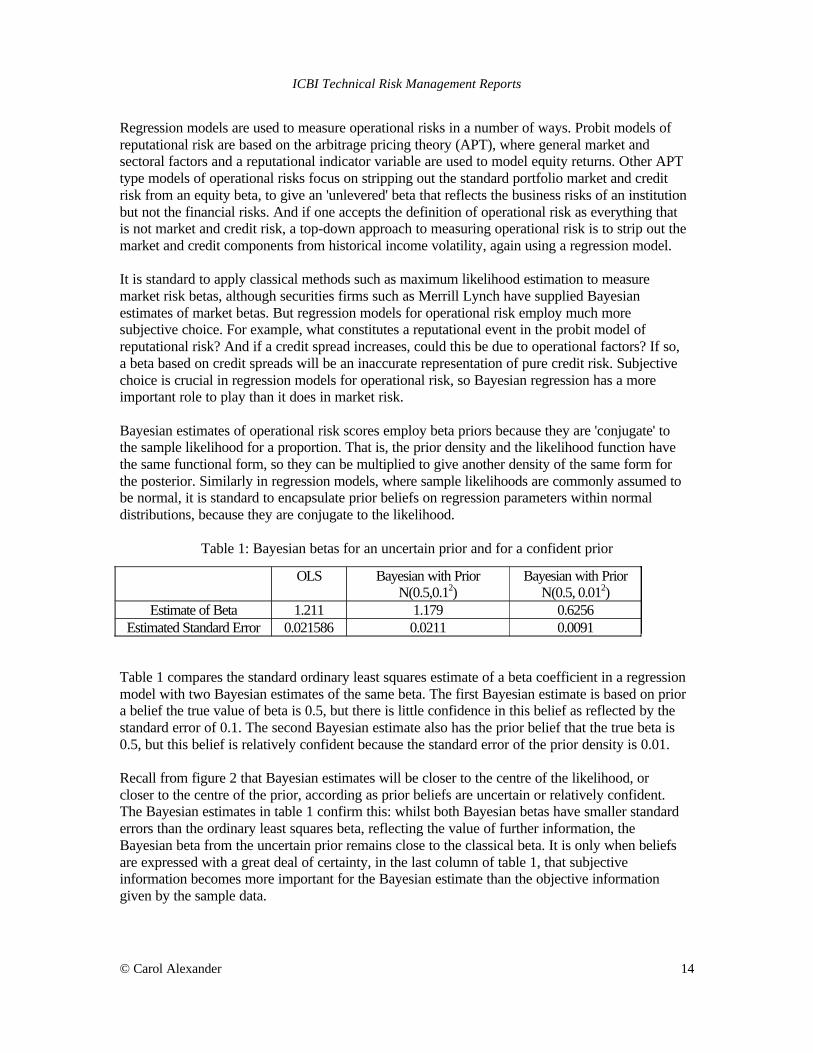
Table 1: Bayesian betas for an uncertain prior and for a confident prior

Table 1 compares the standard ordinary least squares estimate of a beta coefficient in a regression model with two Bayesian estimates of the same beta. The first Bayesian estimate is based on prior a belief the true value of beta is 0.5, but there is little confidence in this belief as reflected by the standard error of 0.1. The second Bayesian estimate also has the prior belief that the true beta is 0.5, but this belief is relatively confident because the standard error of the prior density is 0.01. Recall from figure 2 that Bayesian estimates will be closer to the centre of the likelihood, or closer to the centre of the prior, according as prior beliefs are uncertain or relatively confident. The Bayesian estimates in table 1 confirm this: whilst both Bayesian betas have smaller standard errors than the ordinary least squares beta, reflecting the value of further information, the Bayesian beta from the uncertain prior remains close to the classical beta. It is only when beliefs are expressed with a great deal of certainty, in the last column of table 1, that subjective information becomes more important for the Bayesian estimate than the objective information given by the sample data.

OLS Bayesian with PriorN(0.5,0.12)

Bayesian with PriorN(0.5, 0.012)

Estimate of Beta 1.211 1.179 0.6256Estimated Standard Error 0.021586 0.0211 0.0091



Summary This paper has shown how Bayesian methods may be applied to measure a variety of operational risks, including those that are difficult to quantify such as human risks. Bayesian networks improve transparency for efficient risk management, being based on causal flows in an operational process. A Bayesian network depicts the analyst's view of the process, and so many different network architectures could be built for the same problem. Not only is the architectural design open to subjective choice, in some problems the data itself is very subjective. However Bayesian networks lend themselves very easily to back testing, and to scenario analysis. So the 'best' network design, the most appropriate beliefs about non-quantifiable variables, and the 'maximum operational loss' scenarios can be identified. This helps the operational risk manager to focus on the important factors that influence operational risk. Other examples in this paper have illustrated the advantages of Bayesian estimation over classical estimation for operational risk measurement. From simple operational risk scores to advanced regression models for operational loss, the examples illustrate the power of a Bayesian analyst to influence results. By expressing prior beliefs with more or less uncertainty, the objective information from sample data may be more or less over-ruled. Clearly some balance needs to be achieved between the use of subjective and objective information and this can only be achieved by a thorough model back testing.

References Greene, W.H. (1993) 'Econometric Analysis' (2nd ed, MacMillan) Hoffman, D.G. ed (1998) 'Operational Risk and Financial Institutions' (Risk Publications) ISDA/BBA/RMA survey report (February 2000) 'Operational Risk - The Next Frontier' available from www.isda.org Jensen, F.V. (1996) An Introduction to Bayesian Networks (Springer Verlag). Pearl, J. (1988) Probabilistic Reasoning in Intelligent Systems (Morgan Kaufmann) Useful Websites: http://www.cs.pitt.edu/~tsamard/bnpointers.html

http://www.research.microsoft.com/research.dtg/msbn/default.htm http.cs.berkeley.edu/~murphyk/Bayes/bnsoft.html

Documents

Bayesian Methods for Measuring Operational Risks regulators and the financial services industry in their quest to construct meaningful measures for operational risks