Bayesian Data Analysis - Arizona State Universityjtaylor/teaching/Spring2017/BIO545/... · Bayesian Analysis Bayesian Data Analysis: Overview Bayesian data analysis is based on the

Bayesian Analysis

Bayesian Data Analysis: Overview

Bayesian data analysis is based on the following two principles:

1 Probability is interpreted as a measure of uncertainty, whatever the source.Thus, in a Bayesian analysis, it is standard practice to assign probabilitydistributions not only to unseen data, but also to parameters, models, andhypotheses.

2 Uncertainty is quantified both before and after the collection of data andBayes’ formula is used to update our beliefs in light of the new data.

Jay Taylor (ASU) Bayesian Analysis 30 Jan 2017 1 / 37

Bayesian Analysis

Suppose that our objective is to use some newly acquired data D to estimate the valueof an unknown parameter Θ. A Bayesian treatment of this problem would proceed asfollows:

1 We first need to formulate a statistical model which determines the conditionaldistribution of the data under each possible value of Θ. This is specified bythe likelihood function, p(D|Θ = θ).

2 We then choose a prior distribution, p(Θ = θ), for the unknown parameterwhich quantifies how strongly we believe that the true value is θ before weexamine the new data.

3 We then collect and examine the new data D.

4 In light of this new data, we use Bayes’ formula to revise our beliefs concerningthe value of the parameter Θ:

p(Θ = θ|D)︸︷︷︸posterior

= p(Θ = θ)︸︷︷︸prior

·(p(D|Θ = θ)

p(D)

)

p(Θ = θ|D) is said to be the posterior distribution of the parameter Θ giventhe data D.


Bayesian Analysis

Example: Bayesian Estimation of Sex RatiosSuppose that our objective is to estimate the birth sex ratio of a newly described species.To this end, we will count the numbers of male and female offspring in each of b broods.

For the sake of the example, we will make the following assumptions:

The probability of being born female does not vary within or between broods.In particular, there is no environmental or heritable variation in sex ratio.

The sexes of the different members of a brood are determined independentlyof one another.

If we let θ denote the unknown probability that an individual is born female,then the sex ratio at birth will be θ/1− θ.

We will let m and f denote the total numbers of male and female offspringcontained in the b broods.


Bayesian Analysis

Likelihood Function: Under our assumptions about sex determination, the likelihoodfunction depends only on the sex ratio and the total numbers of males and females inthe broods. Conditional on Θ = θ, the total number of female offspring among the noffspring is binomially distributed with parameters f + m and θ:

Likelihood function

P(f ,m|Θ = θ) =

(f + m

f

)θf (1− θ)m

MLE

θMLE =f

f + m0 0.1 0.2 0.3 0.4 0.5 0.6 0.7 0.8 0.9 10

0.05

0.1

0.15

0.2

0.25

θ

p(3,7|θ

θMLE =0.7

LikelihoodFunction: f=7,m=3


Bayesian Analysis

Prior Distribution: The prior distribution on the unknown parameter θ should reflectwhat we have previously learned about the birth sex ratio in this species. For example,this might be determined by prior observations of this species or by information aboutthe sex ratio of closely-related species. Here I will consider prior distributions for threedifferent scenarios:

Uniform: no prior information

p(Θ = θ) = 1

Beta(5,5): even sex ratio

p(Θ = θ) = 630 θ4(1− θ)4

Beta(2,4): male-biased

p(Θ = θ) = 20 θ(1− θ)3

0 0.1 0.2 0.3 0.4 0.5 0.6 0.7 0.8 0.9 10

0.5

1

1.5

2

2.5

θ

prior

PriorDistributions

Beta(1,1)Beta(5,5)Beta(2,4)


Bayesian Analysis

We are now ready to use Bayes’ formula to calculate the posterior distribution of θconditional on having observed f female offspring out of a total of n offspring. Whenthe prior distribution is of type Beta(a, b), we have

p(Θ = θ|f ,m) = p(Θ = θ) ·(P(f ,m|θ)

P(f ,m)

)(Bayes’ formula)

=1

β(a, b)θa−1(1− θ)b−1 ·

((f +mf

)θf (1− θ)m

P(f ,m)

)

=1

β(f + a,m + b)θf +a−1(1− θ)m+b−1,

which shows that the posterior distribution is of type Beta(f + a,m + b).

RemarkBecause the prior and the posterior distribution belong to the same family ofdistributions, we say that the beta distribution is a conjugate prior for the binomiallikelihood function.


Bayesian Analysis

The figures show the posterior distributions corresponding to each of these three priorsfor two different data sets: either f = 7,m = 3 (left plot) or f = 70,m = 30 (right plot).

0 0.2 0.4 0.6 0.8 10

0.5

1

1.5

2

2.5

3

3.5

4

posteriordensity

PosteriorDistribution: f=7,m=3


0 0.2 0.4 0.6 0.8 10

1

2

3

4

5

6

7

8

9

posteriordensity

PosteriorDistribution: f=70,m=30



Bayesian Analysis

Summaries of the Posterior DistributionAlthough the posterior distribution p(Θ = θ|D) comprehensively describes the stateof knowledge concerning an unknown parameter, it is common to summarize thisdistribution by a number or an interval.

Point estimators of Θ include the mean and the median of the posteriordistribution.

If it exists, the mode of the posterior distribution can be used to estimateΘ, in which case it is called the maximum a posteriori (MAP) estimate.

A credible region is a region that contains a specified proportion of theprobability mass of the posterior distribution, e.g., a 95% credible region

will contain 95% of this mass. These can be chosen in several ways, including:

quantile-based intervals;

highest probability density (HPD) regions.


Bayesian Analysis

Posterior Summary Statistics

Credible Intervals for N(0,1)

MAP = mean = median

95% HPD/quantiles (-1.96, 1.96)

MAP = mean = median = 095% median = (−1.96, 1.96) 95% HPD

= (−1.96, 1.96)

Credible Intervals for Exp(1)

MAP = 0.0

Median = 0.692

Mean = 1.0

95% HPD (0.0, 2.996)

95% quantiles (0.025, 3.69)

MAP = 0, median = 0.692, mean = 1.095% quantiles = (0.025, 3.689)

95% HPD = (0, 2.996)


Bayesian Analysis

The table lists various summary statistics for the posterior distributions calculated in thesex ratio example.

data prior mean median sd 2.5% 97.5%

7, 3 uniform 0.667 0.676 0.131 0.390 0.891even 0.600 0.603 0.107 0.384 0.798♂-biased 0.563 0.565 0.120 0.323 0.787

70, 30 uniform 0.697 0.697 0.045 0.604 0.781even 0.682 0.683 0.044 0.592 0.765♂-biased 0.679 0.680 0.045 0.588 0.764

InterpretationWhereas the small data set does not provide strong evidence against the hypothesis thatthe sex ratio is 1 : 1, all three analyses of the large data set suggest that the true valueof θ is greater than 0.58.


Bayesian Analysis

Acquiring New DataOne of the strengths of Bayesian statistics is that it can readily handle sequentiallyacquired data. This is done by using the posterior distribution from the most recentexperiment as the prior distribution for the next experiment.

p0(θ)︸︷︷︸prior

D1−→ p1(θ) = p0(θ)p(D1|θ)

p(D1)︸︷︷︸posterior


D2−→ p2(θ) = p1(θ)p(D2|θ)

p(D2)︸︷︷︸posterior


D3−→ · · ·


Bayesian Analysis

Example: Sex Ratio Estimation, continuedSuppose that our prior distribution on Θ was uniform and that we initially collectedthree broods totaling 7 females and 3 males. We then used Bayes’ formula to determinethat the posterior distribution of Θ is Beta(8, 4). Since this distribution is broad, wedecide to collect additional data to refine our estimate of Θ.

If the second data set contains 15 females and 5 males, then using Beta(8, 4) as thenew prior distribution, we find that the new posterior distribution of Θ is

p(Θ = θ|f = 15,m = 5) =θ7(1− θ)3

β(8, 4)·

( (2015

)θ15(1− θ)5

P(f = 15,m = 5)

)

=θ22(1− θ)8

β(23, 9)


Bayesian Analysis

Choosing the Prior Distribution: Some GuidelinesChoosing a prior distribution is both useful and sometimes difficult because it requires acareful assessment of our knowledge or beliefs before we perform an experiment.

As a rule, the prior should be chosen independently of the new data.

Cromwell’s rule: The prior distribution should assign positive probabilityto any proposition that is not logically false, no matter how unlikely.

It is sometimes useful to carry out multiple Bayesian analyses using differentprior distributions to explore the sensitivity of the posterior distribution todifferent prior assumptions.

When there is very little prior information, it may be appropriate to choosean “uninformative prior”. Examples include maximum entropy distributionsand Jeffreys priors.


Bayesian Analysis

Bayesian Phylogenetics

Bayesian methods have proven to be especially useful in the analysis of genetic sequencedata. In these problems, the unknown parameters can often be divided into threecategories:

the unknown tree, Tthe parameters of the demographic model, Θdem

the parameters of the substitution model, Θsubst .

Then, given a sequence alignment D, the analytical problem is to calculate the posteriordistribution of all of the unknowns:

Bayes’ formula for phylogenetic inference, general case

p(T ,Θdem,Θsubst |D) = p(T ,Θdem,Θsubst) ·(p(D|T ,Θdem,Θsubst)

p(D)

)


Bayesian Analysis

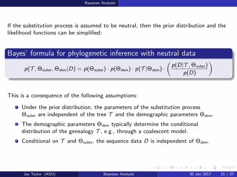
If the substitution process is assumed to be neutral, then the prior distribution and thelikelihood functions can be simplified:

Bayes’ formula for phylogenetic inference with neutral data

p(T ,Θsubst ,Θdem|D) = p(Θsubst) · p(Θdem) · p(T |Θdem) ·(p(D|T ,Θsubst)

p(D)

)

This is a consequence of the following assumptions:

Under the prior distribution, the parameters of the substitution processΘsubst are independent of the tree T and the demographic parameters Θdem.

The demographic parameters Θdem typically determine the conditionaldistribution of the genealogy T , e.g., through a coalescent model.

Conditional on T and Θsubst , the sequence data D is independent of Θdem.


Bayesian Analysis

Example: Bayesian Inference of Effective Population SizeSuppose that our data D consists of n randomly sampled individuals that have beensequenced at a neutral locus and that our objective is to estimate the effectivepopulation size Ne . For simplicity, we will use the Jukes-Cantor model for thesubstitution process with a strict molecular clock and we will assume that thedemography can be described by the constant population size coalescent.

To carry out a Bayesian analysis, we need to specify p(µ), p(Ne) and p(T |Ne).

p(µ) should be chosen to reflect what we know about the mutation rate,e.g., we could use a lognormal distribution with mean u and variance σ2.

Since Ne is a scale parameter in the coalescent, it is common practice touse the Jeffreys prior p(Ne) ∝ 1/Ne .

p(T |Ne) is then determined by Kingman’s coalescent.


Bayesian Analysis

Assuming that we are only interested in Ne , then µ and T are nuisance parameters andso we need to calculate the marginal posterior distribution of Ne by integrating over µand T :

p(Ne |D) =

∫ ∫p(T ,Ne , µ|D)dµdT

=p(Ne)

p(D)

∫ ∫p(D|T , µ)p(µ)p(T |NE )dµdT .

However, unless n is quite small, integration over T is not feasible. For example, if oursample contains 20 sequences, then there are approximately 8× 1021 possible trees to beconsidered. Even with the fastest computers available, this is an impossible calculation.


MCMC

Markov Chain Monte Carlo Methods (MCMC)

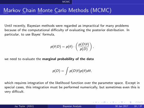
Until recently, Bayesian methods were regarded as impractical for many problemsbecause of the computational difficulty of evaluating the posterior distribution. Inparticular, to use Bayes’ formula,

p(θ|D) = p(θ) ·(p(D|θ)

p(D)

),

we need to evaluate the marginal probability of the data

p(D) =

∫p(D|θ)p(θ)dθ,

which requires integration of the likelihood function over the parameter space. Except inspecial cases, this integration must be performed numerically, but sometimes even this isvery difficult.


MCMC

An alternative is to use Monte Carlo methods to sample from the posterior distribution.Here the idea is to generate a random sample from the distribution and then use theempirical distribution of that sample to approximate p(θ|D):

p(θ|D)︸︷︷︸posterior

≈ 1

N

N∑i=1

δΘi︸︷︷︸empirical distribution

where Θ1, · · · ,ΘN︸︷︷︸sample

∼ p(θ|D)

For example, the figure shows two histogram estimators for the Beta(8, 4) densitygenerated using either 100 (left) or 1000 (right) independent samples:

0 0.2 0.4 0.6 0.8 10

0.5

1

1.5

2

2.5

3

3.5

4

θ

posteriordensity

sample: N =100Beta(8,4)

0 0.2 0.4 0.6 0.8 10

0.5

1

1.5

2

2.5

3

3.5

4

θ

posteriordensity

sample: N =1000Beta(8,4)


MCMC

In particular, the empirical distribution can be used to estimate probabilities andexpectations under p(θ|D):

P(θ ∈ A|D) ≈ 1

N

N∑i=1

1A(Θi )

E[f (θ)|D] ≈ 1

N

N∑i=1

f (Θi ).

What makes this approach difficult is the need to generate random samples fromdistributions that are only known up to a constant of proportionality (e.g., p(D)).This is where Markov chain Monte Carlo methods come in.


MCMC

Markov ChainsA discrete-time Markov chain is a stochastic process X0,X1, · · · with the property thatthe future behavior of the process only depends on its current state. More precisely, thismeans that for every set A and t, s ≥ 0,

P(Xt+s ∈ A︸︷︷︸future

| Xt︸︷︷︸present

,Xt−1, · · · ,X0︸︷︷︸past

) = P(Xt+s ∈ A|Xt).

0 20 40 60 80 100 120 140 160 180 2000

0.1

0.2

0.3

0.4

0.5

0.6

0.7

0.8

0.9

1

time

frequency

Simulations of theWright−FisherProcess

past future

present

N=500,µ=0.001

Markov chains have numerous applicationsin biology. Some familiar examples include:

random walks

branching processes

the Wright-Fisher model

chain-binomial models (Reed-Frost)


MCMC

One consequence of the Markov property is that many Markov chains have a tendencyto ‘forget’ their initial state as time progresses. More precisely,

Asymptotic behavior of Markov chainsMany Markov chains have the property that there is a probability distribution π, calledthe stationary distribution of the chain, such that for large t the distribution of Xt

approaches π, i.e., for all states x and sets A,

limt→∞

P(Xt ∈ A|X0 = x) = π(A).

Stationary behavior of theWright-Fisher process:(N = 100, µ = 0.02)

0 0.5 10

0.02

0.04

0.06

0.08

0.1

0.12

0.14

0.16

p

density

t=2

0 0.5 10

0.005

0.01

0.015

0.02

0.025

0.03

0.035

p

density

t=20

0 0.5 10

0.005

0.01

0.015

0.02

0.025

p

density

t=100

p = 0.01

p = 0.5

p = 0.9


MCMC

Some Markov chains satisfy an even stronger property, called ergodicity.

ErgodicityA Markov chain with stationary distribution π is said to be ergodic if for every initialstate X0 = x and every set A, we have

limT→∞

1

T

T∑t=1

1A(Xt) = π(A).

In other words, if we run the chain for a long time, then the proportion of time spentvisiting the set A is approximately π(A).

Ergodic behavior of theWright-Fisher process:(N = 100, µ = 0.02)

0 1 2 3 4 5 6 7 8 9 10

x104

0

0.1

0.2

0.3

0.4

0.5

0.6

0.7

0.8

0.9

1Neutral Wright−Fishermodel

Generation

p


MCMC

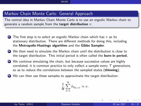
Markov Chain Monte Carlo: General ApproachThe central idea in Markov Chain Monte Carlo is to use an ergodic Markov chain togenerate a random sample from the target distribution π.

1 The first step is to select an ergodic Markov chain which has π as itsstationary distribution. There are different methods for doing this, includingthe Metropolis-Hastings algorithm and the Gibbs Sampler.

2 We then need to simulate the Markov chain until the distribution is close tothe target distribution. This initial period is often called the burn-in period.

3 We continue simulating the chain, but because successive values are highlycorrelated, it is common practice to only collect a sample every T generations,so as to reduce the correlations between the sampled states (thinning).

4 We can then use these samples to approximate the target distribution:

1

N

N∑n=1

δXB+nT ≈ π.


MCMC

The Metropolis-Hastings AlgorithmGiven a probability distribution π, the Metropolis-Hastings algorithm can be used toexplicitly construct a Markov chain that has π as its stationary distribution.

Implementation requires the following elements:

the target distribution, π, known up to a constant of proportionality;

a family of proposal distributions, Q(y |x), and a way to efficiently samplefrom these distributions.

The MH algorithm is based on a more general idea known as rejection sampling.Instead of sampling directly from π, we propose values using a distribution Q(y |x)that we can easily sample but then we reject values that are unlikely under π.


MCMC

The Metropolis-Hastings algorithm consists of repeated application of the followingthree steps. Suppose that Xn = x is the current state of the Markov chain. Then thenext state is chosen as follows:

Step 1: We first propose a new value for the chain by sampling y with probabilityQ(y |x).

Step 2: We then calculate the acceptance probability of the new state:

α(x ; y) = min

{π(y)Q(x |y)

π(x)Q(y |x), 1

}

Step 3: With probability α(x ; y), set Xn+1 = y . Otherwise, set Xn+1 = x .

RemarkBecause π enters into α as a ratio π(y)/π(x), we only need to know π up to a constantof proportionality. This is why the MH algorithm is so well suited for Bayesian analysis.


MCMC

The Proposal DistributionThe choice of the proposal distribution Q can have a profound impact on theperformance of the MH algorithm. While there is no universal procedure for selectinga ‘good’ proposal distribution, the following considerations are important.

Q should be chosen so that the chain rapidly converges to its stationarydistribution.

Q should also be chosen so that it is easy to sample from.

There is usually a tradeoff between these two conditions and sometimes it isnecessary to try out different proposal distributions to identify one with goodproperties.

Many implementations of MH (e.g., BEAST, MIGRATE) offer the user some controlover the proposal distribution.


MCMC

MCMC: Convergence and MixingOne of the most challenging issues in MCMC is knowing for how long to run the chain.There are two related considerations.

1 We need to run the chain until its distribution is sufficiently close to thetarget distribution (convergence).

2 We then need to collect a large enough number of samples that we canestimate any quantities of interest (e.g., the mean TMRCA) sufficientlyaccurately (mixing).

Unfortunately, there is no universally-valid, fool-proof way to guarantee that eitherone of these conditions is satisfied. However, there are a number of convergencediagnostics that can indicate when there are problems.


MCMC

Convergence Diagnostics: Trace Plots

Trace plots show how the value of a parameter changes over the course of a simulation.In general, what we want to see is that the mean and the variance of the parameter arefairly constant over the duration of the trace plot, as in the two examples shown below.

P_

viva

x_g

sr_

ge

o1

.log

State

0 10000000 2E7 3E7 4E71600

1650

1700

1750

1800

1850

1900

1950

2000

P_

viva

x_g

sr_

ge

o1

.log

State

0 10000000 2E7 3E7 4E70

1

2

3

4

5

6


MCMC

Problems with convergence or mixing may be revealed by trends or sudden changes inthe behavior of the trace plot.

P_

viva

x_g

sr_

ge

o1

.log

State

0 10000000 2E7 3E7 4E7-750

-700

-650

-600

-550

-500

The increasing trend indicates that thechain has not yet converged.

P_

viva

x_g

sr_

ge

o1

.log

State

0 10000000 2E7 3E7 4E7-7450

-7425

-7400

-7375

-7350

-7325

-7300

The sudden changes in mean indicate thatthe chain is poorly mixing.


MCMC

Trace Plots: Some Guidelines

1 You should examine the trace plot of every parameter of interest, includingthe likelihood and the posterior probability. If any of the trace plots lookproblematic, then all of the results are suspect.

2 The fact that a trace plot appears to have converged is not conclusive proofthat it has. Especially in high-dimensional problems, a chain that appears tobe stationary for the first 500 million generations may well show a suddenchange in behavior in the next.

3 The program Tracer (http://tree.bio.ed.ac.uk/software/tracer/)can be used to display and analyze trace plots generated by BEAST, MrBayesand LAMARC.


http://tree.bio.ed.ac.uk/software/tracer/

MCMC

Convergence Diagnostics: Effective Sample Size

Because successive states visited by a Markov chain are correlated, an estimate derivedusing N values generated by such a chain will usually be less precise than an estimatederived using N independent samples. This motivates the following definition.

Effective Sample Size (ESS)

The effective sample size of a sample of N correlated random variables is equal to thenumber of independent samples that would estimate the mean with the same variance.

For a stationary Markov chain with autocorrelation coefficients ρk , the ESS of Nsuccessive samples is equal to

ESS =N

1 + 2∑∞

k=1 ρk.


MCMC

Effective Sample Size: Guidelines

1 Each parameter has its own ESS and these can differ between parametersby more than order of magnitude.

2 Parameters with small ESS’s indicate that a chain either has not convergedor is slowly mixing. As a rule of thumb, the ESS of every parameter shouldexceed 1000 and larger values are even better.

3 Thinning by itself will not increase the ESS. However, we can increase theESS by simultaneously thinning and increasing the duration of the chain,e.g., collecting a 1000 samples from a chain lasting 100000 generations isbetter than collecting a 1000 samples from a chain lasting 10000 generations.

4 The ESS of a parameter can usually only be estimated from its trace. Forthis reason, large ESS’s do not guarantee that the chain has converged.


MCMC

Formal Tests of Convergence

There are several formal tests of stationarity that can be applied to MCMC.

The Geweke diagnostic compares the mean of a parameter estimatedfrom two non-overlapping parts of the chain and tests whether these aresignificantly different.

The Raftery-Lewis diagnostic uses a pilot chain to estimate the burn-inand chain length required to estimate the q’th quantile of a parameter towithin some tolerance.

Both of these methods suffer from the defect that “you’ve only seen whereyou’ve been” (Robert & Casella, 2004). In other words, these methodscannot detect that the chain has failed to visit part of the support of thetarget distribution.

These and other diagnostic tests are implemented in the R package coda.


MCMC

Convergence Diagnostics: Multiple Chains

Another approach to testing the convergence of a MCMC analysis is to run multipleindependent chains and compare the results.

Large differences between the posterior distributions estimated by the differentchains indicate problems with convergence or mixing.

It is often useful to start the different chains from different, randomly-choseninitial conditions.

If the different chains give similar results, then their traces can be combinedusing a program such as LogCombiner (http://beast2.org).

Best PracticeIt is always a good idea to run at least two independent chains in any MCMC analysis.


http://beast2.org

MCMC

Metropolis-Coupled Markov Chain Monte Carlo (MC3)

MC3 is a generalization of MCMC which attempts to improve mixing by running mchains in parallel, while randomly exchanging their states.

The first chain (the cold chain) is constructed so that the target distributionπ is its stationary distribution.

The i ’th chain is constructed so that its stationary distribution is proportional to

πi (x) ∝ π(x)1/Ti

where Ti is said to be the temperature of the chain. As Ti increases, thedistribution πi (x) becomes flatter, which makes it easier for this chain to converge.

The MH algorithm is used to swap the states occupied by different chains insuch a way that the stationary distribution of each chain is maintained.

The output from the cold chain is then used to approximate the target distribution.


MCMC

References I

M. A. Beaumont and B. Rannala, The Bayesian revolution in genetics, Nat. Rev.Genetics 5 (2004), 251–261.

A. Gelman, J. B. Carlin, H. S. Stern, and D. B. Rubin, Bayesian Data Analysis,second ed., Chapman & Hall/CRC, 2004.

P. Gregory, Bayesian Logical Data Analysis for the Physical Sciences, CambridgeUniversity Press, 2010.

P. Lemey, M. Salemi, and A.-M. Vandamme (eds.), The Phylogenetic Handbook:A Practical Approach to Phylogenetic Analysis and Hypothesis Testing, second ed.,Cambridge University Press, 2009.

S. P. Otto and T. Day, A Biologist’s Guide to Mathematical Modeling in Ecologyand Evolution, Princeton University Press, 2007.

C. P. Robert and G. Casella, Monte Carlo Statistical Methods, Springer-Verlag,2004.


Documents

Bayesian Data Analysis - Arizona State Universityjtaylor/teaching/Spring2017/BIO545/... · Bayesian Analysis Bayesian Data Analysis: Overview Bayesian data analysis is based on the