Bayesact I - Background

Jesse Hoey

February 6, 2014

Readings:

M.Sanjeev Arulampalam, Simon Maskell, Neil Gordon andTim Clapp. A tutorial on particle filters for onlinenonlinear/non-Gaussian Bayesian tracking. IEEE Transactionson Signal Processing, Vol 50, No 2, Feb 2002.David Silver and Joel Veness Monte Carlo Planning in LargePOMDPs. In NIPS 2010.

Background: David Poole and Alan Mackworth. Artificial Intelligence:

Foundations of Computational Agents. Cambridge University Press,

2010. Chapters 6 and 9 in particular. See artint.info

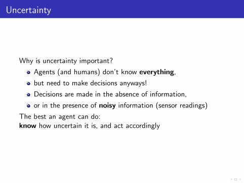
Uncertainty

Why is uncertainty important?

Agents (and humans) don’t know everything,

but need to make decisions anyways!

Decisions are made in the absence of information,

or in the presence of noisy information (sensor readings)

The best an agent can do:know how uncertain it is, and act accordingly

Probability: Frequentist vs. Bayesian

Frequentist view:probability of heads = # of heads / # of flipsprobability of heads this time = probability of heads (history)Uncertainty is ontological: pertaining to the world

Bayesian view:probability of heads this time = agent’s belief about this eventbelief of agent A : based on previous experience of agent AUncertainty is epistemological: pertaining to knowledge

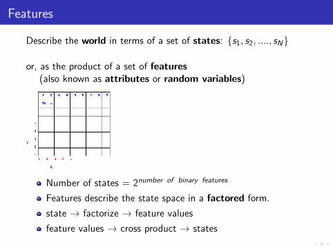
Features

Describe the world in terms of a set of states: {s1, s2, ...., sN}

or, as the product of a set of features(also known as attributes or random variables)

Number of states = 2number of binary features

Features describe the state space in a factored form.

state → factorize → feature values

feature values → cross product → states

Probability Measure

if X is a random variable (feature, attribute),it can take on values x , where x ∈ Domain(X )Pr(X = x) ≡ Pr(x) is the probability that X = xjoint probability Pr(X = x ,Y = y) ≡ Pr(x , y) is the

probability that X = x and Y = y at the same timeJoint probability distribution:

Sum Rule: ∑x

Pr(X = x ,Y ) = Pr(Y )

We call Pr(Y ) the marginal distribution over Y

Independence

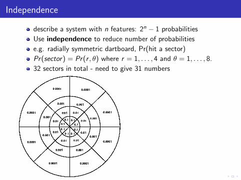
describe a system with n features: 2n − 1 probabilities

Use independence to reduce number of probabilities

e.g. radially symmetric dartboard, Pr(hit a sector)

Pr(sector) = Pr(r , θ) where r = 1, . . . , 4 and θ = 1, . . . , 8.

32 sectors in total - need to give 31 numbers

Independence

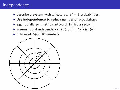
describe a system with n features: 2n − 1 probabilities

Use independence to reduce number of probabilities

e.g. radially symmetric dartboard, Pr(hit a sector)

assume radial independence: Pr(r , θ) = Pr(r)Pr(θ)

only need 7+3=10 numbers

Independence

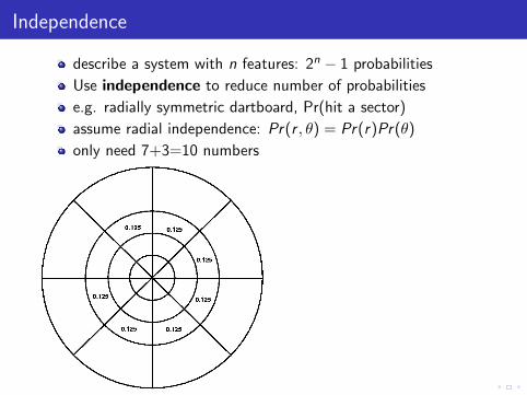
describe a system with n features: 2n − 1 probabilities

Use independence to reduce number of probabilities

e.g. radially symmetric dartboard, Pr(hit a sector)

assume radial independence: Pr(r , θ) = Pr(r)Pr(θ)

only need 7+3=10 numbers

Conditional Probability

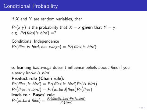
if X and Y are random variables, then

Pr(x |y) is the probability that X = x given that Y = y .e.g. Pr(flies|is bird) =?

Conditional IndependencePr(flies|is bird , has wings) = Pr(flies|is bird)

so learning has wings doesn’t influence beliefs about flies if youalready know is birdProduct rule (Chain rule):Pr(flies, is bird) = Pr(flies|is bird)Pr(is bird)Pr(flies, is bird) = Pr(is bird |flies)Pr(flies)leads to : Bayes’ rulePr(is bird |flies) = Pr(flies|is bird)Pr(is bird)

Pr(flies)

Conditional Probability

if X and Y are random variables, then

Pr(x |y) is the probability that X = x given that Y = y .e.g. Pr(flies|is bird) =?

Conditional IndependencePr(flies|is bird , has wings) = Pr(flies|is bird)

so learning has wings doesn’t influence beliefs about flies if youalready know is birdProduct rule (Chain rule):Pr(flies, is bird) = Pr(flies|is bird)Pr(is bird)Pr(flies, is bird) = Pr(is bird |flies)Pr(flies)leads to : Bayes’ rulePr(is bird |flies) = Pr(flies|is bird)Pr(is bird)

Pr(flies)

Why is Bayes’ theorem interesting?

Often you have causal knowledge:Pr(flies | is bird)Pr(symptom | disease)Pr(alarm | fire)

Pr(image looks like | a tree is in front of a car)

and want to do evidential reasoning:Pr(is bird | flies)Pr(disease | symptom)Pr(fire | alarm).

Pr(a tree is in front of a car | image looks like )

Updating belief: Bayes’ Rule

Agent has a prior belief in a hypothesis, h, Pr(h),

Agent observes some evidence ethat has a likelihood given the hypothesis: Pr(e|h).

The agent’s posterior belief about h after observing e, Pr(h|e),

is given by Bayes’ Rule:

Pr(h|e) =Pr(e|h)Pr(h)

Pr(e)=

Pr(e|h)p(h)∑h Pr(e|h)Pr(h)

Expected Values

expected value of a function on X , V (X ):

EPr(x)(V ) =∑

x∈Dom(X ) Pr(x)V (x)

where Pr(x) is the probability that X = x .

This is useful in decision making, where V (X ) is the utility ofsituation X .

Bayesian decision making is then

arg maxdecision

EPr(outcome|decision)(V (decision))

= arg maxdecision

∑outcome

Pr(outcome|decision)V (outcome)

Value of Independence

complete independence reduces both representation andinference from O(2n) to O(n)

Unfortunately , complete mutual independence is rare

Fortunately , most domains do exhibit a fair amount ofconditional independence

Bayesian Networks or Belief Networks (BNs) encode thisinformation

Bayesian Networks

A Bayesian Network (Belief Network, Probabilistic Network) orBN over variables {X1,X2, . . . ,XN} consists of:

a DAG whose nodes are the variables

a set of Conditional Probability tables (CPTs) givingPr(Xi |Parents(Xi )) for each Xi

Video 2 (V2)

Behavior (B)Mood (M)

Face (F)

Video 1 (0)

B

v2

smile

yell 0.9 0.1

0.90.1

E

neutral

angry

sad

happy

Emotion (E)

B Pr(B)

yell 0.1

0.9smile

BM

good yell

bad yell .01 .4 .09 .5

.01 .88 .1 .01

bad smile .4 .09 .5 .01

h s a n

good smile .88 .01 .01 .1

happy sad angry neutralE

0.85 0.05

0.85

0.85

0.85

0.05

0.05

0.05

0.05

0.05

0.05

0.05

0.050.05

0.05

0.05

neutral

F

smile

cry

frown

F

smile cry frown neutral

0.7

0.5

0.6 0.4

0.5

0.3

1.0

0

0

00

0

0

0

0

0

0

M Pr(M)

good 0.8

0.2bad

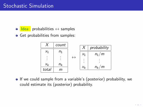
Stochastic Simulation

Idea: probabilities ↔ samples

Get probabilities from samples:

X count

x1 n1...

...xk nk

total m

↔

X probability

x1 n1/m...

...xk nk/m

If we could sample from a variable’s (posterior) probability, wecould estimate its (posterior) probability.

Generating samples from a distribution

For a variable X with a discrete domain or a (one-dimensional) realdomain:

Totally order the values of the domain of X .

Generate the cumulative probability distribution:f (x) = Pr(X ≤ x).

Select a value y uniformly in the range [0, 1].

Select the x such that f (x) = y .

0

1

v1 v2 v3 v4 v1 v2 v3 v4

P(X)

f(X)

0

1

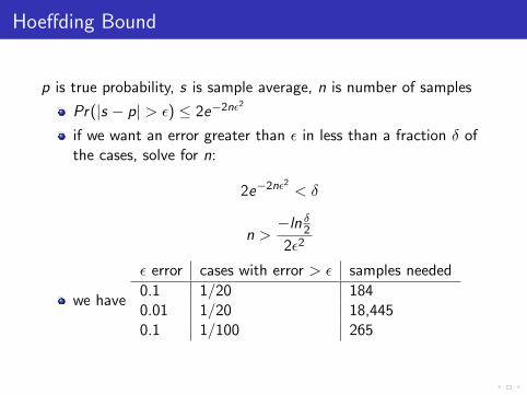
Hoeffding Bound

p is true probability, s is sample average, n is number of samples

Pr(|s − p| > ε) ≤ 2e−2nε2

if we want an error greater than ε in less than a fraction δ ofthe cases, solve for n:

2e−2nε2 < δ

n >−ln δ22ε2

we have

ε error cases with error > ε samples needed

0.1 1/20 1840.01 1/20 18,4450.1 1/100 265

Forward sampling in a belief network

Sample the variables one at a time; sample parents of Xbefore you sample X .

Given values for the parents of X , sample from the probabilityof X given its parents.

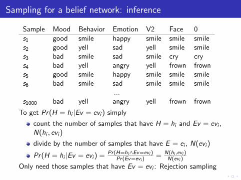
Sampling for a belief network: inference

Sample Mood Behavior Emotion V2 Face 0

s1 good smile happy smile smile smiles2 good yell sad yell smile smiles3 bad smile sad smile cry crys4 bad yell angry yell frown frowns5 good smile happy smile smile smiles6 bad smile sad smile smile smile

...s1000 bad yell angry yell frown frown

To get Pr(H = hi |Ev = evi ) simply

count the number of samples that have H = hi and Ev = evi ,N(hi , evi )

divide by the number of samples that have E = ei , N(evi )

Pr(H = hi |Ev = evi ) = Pr(H=hi∧Ev=evi )Pr(Ev=evi )

= N(hi ,evi )N(evi )

Only need those samples that have Ev = evi : Rejection sampling

Importance Sampling

If we can compute Pr(evidence|sample) we can weight the(partial) sample by this value.

To get the posterior probability, we do a weighted sum overthe samples; weighting each sample by its probability.

We don’t need to sample all of the variables as long as weweight each sample appropriately.

We thus mix exact inference with sampling.

Don’t even have to draw from any true distribution, Pr(B)

Draw from proposal q(B)→ bi ,

additionally weight by Pr(bi )/q(bi )

Importance Sampling

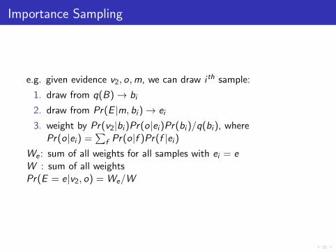
e.g. given evidence v2, o,m, we can draw i th sample:

1. draw from q(B)→ bi

2. draw from Pr(E |m, bi )→ ei

3. weight by Pr(v2|bi )Pr(o|ei )Pr(bi )/q(bi ), wherePr(o|ei ) =

∑f Pr(o|f )Pr(f |ei )

We : sum of all weights for all samples with ei = eW : sum of all weightsPr(E = e|v2, o) = We/W

Probability and Time

A node repeats over time

explicit encoding of time

Chain has length = amount of time you want to model

Event-driven times or Clock-driven times

e.g. Markov chain

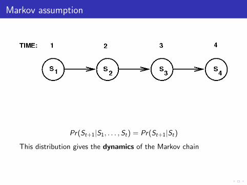
Markov assumption

Pr(St+1|S1, . . . ,St) = Pr(St+1|St)

This distribution gives the dynamics of the Markov chain

Hidden Markov Models (HMMs)

Add: observations Ot andobservation function Pr(Ot |St)Given a sequency of observations O1, . . . ,Ot , can estimatefiltering:

Pr(St |O1, . . . ,Ot)

or smoothing, for k < t

Pr(Sk |O1, . . . ,Ot)

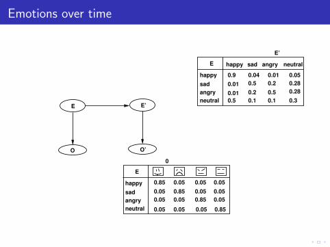
Emotions over time

0.1

0.2

0.010.04 0.05

0.5

O O’

0.28

0.28

0.3

0.5

0.9

0.01

0.01

0.5

0.2

0.1E’

neutralhappy sad

0.85 0.05

0.85

0.85

0.85

0.05

0.05

0.05

0.05

0.05

0.05

0.05

0.050.05

happy

sad

angry

neutral

E

neutral

angry

sad

happy

E

0.05

0.05

0

angry

E’

E

Dynamics Bayesian Networks (DBNs)

Video 2 (V2) Video 2 (V2)

Behavior (B)Behavior (B)Mood (M) Mood (M)

Face (F)Face (F)

Video 1 (0) Video 1 (0)

Emotion (E)

time t time t+1

Emotion (E)

Particle Filtering

Evidence arrives over time:

Particle Filtering

Represent distributions with samples:

Particle Filtering

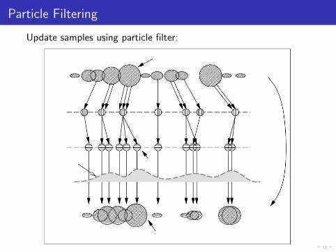
Update samples using particle filter:

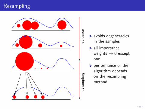
Resampling

resa

mpli

ng

evid

ence

avoids degeneraciesin the samples

all importanceweights → 0 exceptone

performance of thealgorithm dependson the resamplingmethod.

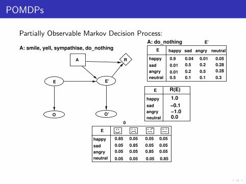
POMDPs

Partially Observable Markov Decision Process:

E

happy

sad

angry

neutral

A

A: smile, yell, sympathise, do_nothing

R(E)

1.0

−0.1−1.00.0

A: do_nothing

R

0.1

0.2

0.010.04 0.05

0.5

O O’

0.28

0.28

0.3

0.5

0.9

0.01

0.01

0.5

0.2

0.1E’

happy sad

0.85 0.05

0.85

0.85

0.85

0.05

0.05

0.05

0.05

0.05

0.05

0.05

0.050.05

0.05

happy

sad

angry

neutral

E

neutral

angry

sad

happy

E

0.05

0

angry

E’

neutral

E

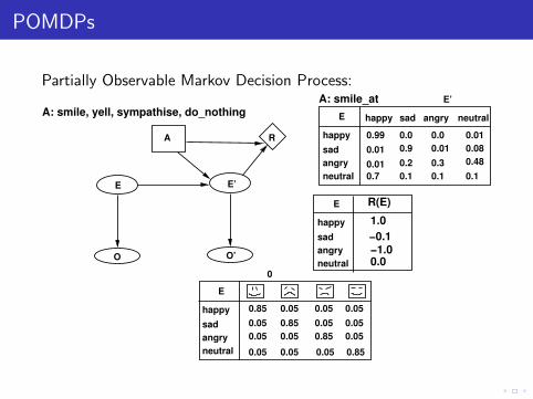
POMDPs

Partially Observable Markov Decision Process:

0.0

A: smile_at

0.01

0.1 0.1

0.99

0.7

0.0

0.48

0.08

0.01

0.010.90.01

0.30.2

0.1

E

happy

sad

angry

neutral

A

A: smile, yell, sympathise, do_nothing

R(E)

1.0

−0.1−1.00.0

R

O’O

E’

neutralhappy

E E’

sad angry

0.85 0.05

0.85

0.85

0.85

0.05

0.05

0.05

0.05

0.05

0.05

0.05

0.050.05

0.05

0.05

happy

sad

angry

neutral

E

neutral

angry

sad

happy

E

0

POMDPs

Partially Observable Markov Decision Process:

0.5

0.180.70.10.01

0.10.30.2

0.050.010.140.8

0.10.1

0.4

0.3

A: sympathise_with

E

happy

sad

angry

neutral

A

A: smile, yell, sympathise, do_nothing

R(E)

1.0

−0.1−1.00.0

R

O’O

E’

neutralhappy

E E’

sad angry

0.85 0.05

0.85

0.85

0.85

0.05

0.05

0.05

0.05

0.05

0.05

0.05

0.050.05

0.05

0.05

happy

sad

angry

neutral

E

neutral

angry

sad

happy

E

0

Policies

Policy: maps beliefs states into actions π(b(s))→ aTwo ways to compute a policy

1. Backwards searchI Dynamic programming (Variable Elimination)I in MDP:

Qt(s, a) = R(s, a) + γ∑

s′ Pr(s ′|s, a) maxa′ Qt−1(s ′, a′)I in POMDP: Qt(b(s), a)

2. Forwards search : Monte Carlo Tree Search (MCTS)I Expand the search treeI Expand more deeply in promising directionsI Ensure exploration using e.g. UCB

MCTS

Selection Expansion Simulation Backpropagation

Select node to visitbased on tree policy.

A new node is added tothe tree upon selection.

Run trial simulation basedon a default policy (usu-

ally random) from thenewly created node untilterminal node is reached.

Sampled statistics from thesimulated trial is propagated

back up from the childnodes to the ancestor nodes.

Next:

Bayesian Affect Control Theory (I)

Bayesian Affect Control Theory (II)