Baumol’s Cost Disease: A Macroeconomic Perspective · Baumol’s Diseases: A Macroeconomic Perspective William D. Nordhaus NBER Working Paper No. 12218 May 2006 JEL No. D4, O3,

NBER WORKING PAPER SERIES

BAUMOL’S DISEASES: A MACROECONOMIC PERSPECTIVE

William D. Nordhaus

Working Paper 12218http://www.nber.org/papers/w12218

NATIONAL BUREAU OF ECONOMIC RESEARCH1050 Massachusetts Avenue

Cambridge, MA 02138May 2006

The author is grateful for extensive helpful comments from William Baumol and anonymous referees. 2 Forthis working paper, Accompanying Notes are available that describe the equations, the sources, and providea list of data fi les. The note and the underlying files are available athttp://www.econ.yale.edu/~nordhaus/Baumol/. The views expressed herein are those of the author(s) and donot necessarily reflect the views of the National Bureau of Economic Research.

©2006 by William D. Nordhaus. All rights reserved. Short sections of text, not to exceed two paragraphs,may be quoted without explicit permission provided that full credit, including © notice, is given to thesource.

Baumol’s Diseases: A Macroeconomic PerspectiveWilliam D. NordhausNBER Working Paper No. 12218May 2006JEL No. D4, O3, O4

ABSTRACT

William Baumol and his co-authors have analyzed the impact of differential productivity growth onthe health of different sectors and on the overall economy. They argued that technologically stagnantsectors experience above average cost and price increases, take a rising share of national output, andslow aggregate productivity growth. Using industry data for the period 1948-2001, the present studyinvestigates Baumol’s diseases for the overall economy. It finds that technologically stagnant sectorsclearly have rising relative prices and declining relative real outputs. Additionally, technologicallyprogressive sectors tend to have slower hours and employment growth outside of manufacturing.Finally, sectoral shifts have tended to lower overall productivity growth as the share of stagnantsectors has risen over the second half of the twentieth century.

William D. NordhausYale UniversityDepartment of Economics28 Hillhouse AvenueBox 208264New Haven, CT 06520-8264and [email protected]

- 2 -

In a series of pioneering works, William Baumol and his co-

authors have analyzed the impact of differential productivity growth on

the health of different sectors and on the overall economy.3 They

hypothesize that sectors whose productivity-growth rates are below the

economy’s average (call them stagnant) will tend to experience above

average cost increases. The resulting “cost disease” may lead stagnant

sectors to experience above-average price increases, declining quality,

and financial pressures. Additionally, there may be a reduction in the

economy’s overall rate of productivity and real output growth because

of the drag from stagnant sectors. This work suggests that a taste for the

output of stagnant sectors may lead to secular stagnation and declining

real-income growth as consumers increasingly demand labor-intensive

services where productivity growth is intrinsically limited.

Baumol et al. applied these ideas to several sectors, including

higher education, cities, health care and hospitals, the performing arts,

handicrafts, haute cuisine, custom clothing, and stately houses. The

studies provoked a flood of criticisms and analysis on industrial

3 William J. Baumol and William G. Bowen, “On the Performing Arts: The

Anatomy of their Economic Problems.” The American Economic Review, Vol. 55,

No. 2, 1965, pp. 495-502; William J. Baumol and William G. Bowen, Performing

Arts: The Economic Dilemma, New York: The Twentieth Century Fund, 1966;

William J. Baumol, “Macroeconomics of Unbalanced Growth: The Anatomy of

Urban Crisis,” The American Economic Review, Vol. 57, No. 3, June, 1967, pp.

419-420; William J. Baumol, Sue Anne Batey Blackman, and Edward N. Wolff,

“Unbalanced Growth Revisited: Asymptotic Stagnancy and New Evidence,”

The American Economic Review, Vol. 75, No. 4., Sept, 1985, pp. 806-817.

- 3 -

productivity studies, but at the end of the day, it remains difficult to

determine the net result.4

4 Peter S. Albin, “Poverty, Education, and Unbalanced Economic Growth,”

The Quarterly Journal of Economics, Vol. 84, No. 1, Feb., 1970, , pp. 70-84;

Carolyn Shaw Bell, “Macroeconomics of Unbalanced Growth: Comment (in

Communications),” The American Economic Review, Vol. 58, No. 4, Sept., 1968,

pp. 877-884; Albert Breton, “The Growth of Competitive Governments,” The

Canadian Journal of Economics, Vol. 22, No. 4, Nov., 1989, pp. 717-750; Cristina

Echevarria, “Agricultural Development vs. Industrialization: Effects of

Trade,” The Canadian Journal of Economics, Vol. 28, No. 3, Aug., 1995, pp. 631-

647; Cristina Echevarria, “Changes in Sectoral Composition Associated with

Economic Growth,” International Economic Review, Vol. 38, No. 2, May, 1997,

pp. 431-452; Norman Gemmell, “A Model of Unbalanced Growth: The Market

versus the Non-Market Sector of the Economy,” Oxford Economic Papers, Vol.

39, No. 2, June, 1987, pp. 253-267; Charles R. Hulten, “Productivity Change in

State and Local Governments,” The Review of Economics and Statistics, Vol. 66,

No. 2, May, 1984, pp. 256-266; William D. Nordhaus, “The Recent

Productivity Slowdown,” Brookings Papers on Economic Activity, 3:1972, pp.

493-536; Joan Robinson, “Macroeconomics of Unbalanced Growth: A Belated

Comment (in Communications),” The American Economic Review, Vol. 59, No.

4., Sept., 1969, p. 632; David Throsby, “The Production and Consumption of

the Arts: A View of Cultural Economics,” Journal of Economic Literature, Vol.

32, No. 1, Mar., 1994, pp. 1-29; Jack E. Triplett and Barry P. Bosworth, “

‘Baumol's Disease’ Has Been Cured,” Federal Reserve Bank of New York

Economic Policy Review, September 2003, pp. 23-33; Edward N. Wolff,

“Industrial Composition, Interindustry Effects, and the U.S. Productivity

Slowdown,” The Review of Economics and Statistics, Vol. 67, No. 2, May, 1985,

pp. 268-277; Michael C. Wolfson, “New Goods and the Measurement of Real

Economic Growth,” The Canadian Journal of Economics, Vol. 32, No. 2, Special

- 4 -

The purpose of this study is to analyze various Baumol-type

diseases using detailed data on economic activity by industry. This

reevaluation is motivated by the availability of more comprehensive

data on output, prices, and productivity by industry as well as by

improved approaches to measuring price and output indexes. The

discussion proceeds in five sections. The first section describes briefly

the different Baumol-related diseases that will be examined. The second

section lays out an analytical framework for examining Baumol’s

diseases, while the following section describes the data used for the

analysis. The fourth section applies the theory and data to examine the

impact of differential productivity growth by sector on the structure of

industry and examines the impact of the cost disease on the economy’s

overall rate of productivity. The final section summarizes the results.

I. Variants of Baumol Diseases

There are several syndromes that might arise from differential

rates of productivity growth. Here are some important ones:

1. Cost and price disease. We would generally expect that average

costs and prices in stagnant industries – ones with relatively low

productivity growth – would grow relative to the average.

Issue on Service Sector Productivity and the Productivity Paradox, Apr., 1999,

pp. 447-470.

- 5 -

2. Stagnating real output. Additionally, because of the rapid rise in

relative prices, we would expect that real output in low-productivity-

growth industries would grow slowly relative to the overall economy.

3. Unbalanced growth. The impact of low productivity growth on

nominal shares is ambiguous because it depends on the interaction of

rising relative prices and declining relative outputs. Baumol sometimes

assumed that demand would be price-inelastic, so low productivity

growth would generally lead to rising shares of nominal output in

stagnant industries.

4. Impact on employment and hours. The impact of low productivity

growth on labor inputs will depend on the impact on output as well as

on the structure of production. Generally, those industries with price-

elastic demand for output will experience a positive impact of

productivity growth on employment, and contrariwise for industries

with price-inelastic demand.

5. Impact on factor rewards. An important question concerns who

captures the gains from higher productivity growth, and who loses from

stagnant productivity. In their 1965 article, Bowen and Baumol argued

that stagnant industries such as the performing arts were likely to be

financially stressed because of rising costs and prices. What are the

facts?

6. Impact on aggregate productivity growth. Will stagnant industries

have rising shares of total output? If so, will this tend to reduce overall

growth in productivity and living standards? This important question

will depend upon the composition of output and is an intriguing

question raised by the earlier studies.

II. Analytical Framework for Baumol’s Cost Disease

Most of the early studies of the various Baumol hypotheses used

either a stylized two-sector analysis or Laspeyres output indexes or

both. This section examines the interpretation of the propositions for

many sectors and in the context of current superlative measures of

output.

Assume that the economy is composed of a large number of non-

durable final goods and services. The notation used for different

variables is shown in the accompanying box. The general notation is

that upper-case roman letters represent levels, lower-case roman letters

represent natural logarithms, and Greek letters represent parameters or

random terms. We define the logarithmic growth rate of a variable as a

lower-case roman letter with a circumflex; therefore,

is the growth rate of productivity. )∆ln(A a- aa t1-ttt ==ˆ

We can write a simplified production, cost, supply and demand

structure as follows. Each industry has a Cobb-Douglas value-added

production function in capital, labor, and time-varying exogenous

technology.5 The derivation here uses the growth rates of variables in

- 6 -

5 An alternative approach would be to use total output rather than value

added. This approach has been used, for example, in Dale W. Jorgenson, Mun

Ho, and Kevin J. Stiroh, “Growth of U.S. Industries and Investments in

Information Technology and Higher Education” in Carol Corrado, John

the production and demand functions to be consistent with superlative

output measurement. The exposition assumes that all industries are

vertically integrated. The error term is interpreted as production shocks

(such as measurement errors) that do not enter into costs.

(1) Production: xitε k )β- (1 mβ a x itititititit +++= ˆˆˆˆ

Under the assumption of cost minimization, the unit cost function

is the dual of (1). It excludes the error in (1) but includes random cost

errors. Note that by duality, the production and cost elasticities in (1)

and (2) are identical.

(2) Cost: *zititititititit c )β- (1 wβ a - z ε+++= ˆˆˆˆ

Pricing is assumed to be a markup over cost. In this specification,

marginal and average costs are equal, so no ambiguity arises with

respect to which cost is involved in pricing. The price function may

include monopolistic elements as well as random elements and drift.

(3) Price: pititiiit z γ p εθ ++= ˆˆ

- 7 -

Haltiwanger, and Daniel Sichel, eds., Measuring Capital in the New Economy,

University of Chicago Press, Chicago, 2005. The relative merits of value-added

output and total output are discussed below.

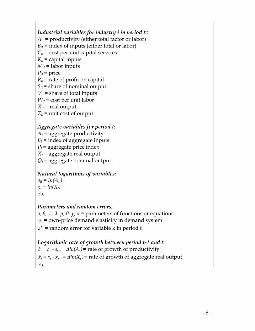
Industrial variables for industry i in period t:: Ait = productivity (either total factor or labor) Bit = index of inputs (either total or labor) Cit= cost per unit capital services Kit = capital inputs Mit = labor inputs Pit = price Rit = rate of profit on capital Sit = share of nominal output Vit = share of total inputs Wit = cost per unit labor Xit = real output Zit = unit cost of output

Aggregate variables for period t: At = aggregate productivity Bt = index of aggregate inputs Pt = aggregate price index Xt = aggregate real output Qt = aggregate nominal output Natural logarithms of variables: ait = ln(Ait) xt = ln(Xt) etc. Parameters and random errors: α, β, γ, λ, µ, θ, χ, σ = parameters of functions or equations

iη = own-price demand elasticity in demand system ktε = random error for variable k in period t

Logarithmic rate of growth between period t-1 and t:

)∆ln(A a- aa t1-ttt ==ˆ = rate of growth of productivity )∆ln(X x- xx t1-ttt ==ˆ = rate of growth of aggregate real output

etc.

- 8 -

The factor shares are determined by the income identity:

(4) Income ititititititit MW K R XP Q +≡≡

Note that the rate of profit on capital includes not only the cost per

unit capital input in (2) but also any returns to market power,

innovation, risk-bearing, and other non-labor returns.

)(Rit

Consumer demand for output from the different sectors is a

variant of the almost ideal demand system, in which expenditure shares

are determined by relative prices and total income.6 In the version used

here, we simplify by assuming that all cross-elasticities of demand are

proportional to output shares; we further have prices and total output

determine the logarithm of the shares. Working in the rates of growth,

and solving for real output growth, we then write the simplified almost

ideal demand system (SAIDS) as:

(5) sittititiiit x )p -p( η λ x εµ +++= ˆˆˆˆ

In this equation, iη is the own price-elasticity of demand for industry i

as a function of the price of that good relative to the aggregate price

index. The logarithmic changes in the aggregate price and output are

Törnqvist indexes, and , where are the

Törnqvist shares of nominal output. We have for notational convenience

∑=

=n

ip

1

ˆˆ ititt S p ∑=

=n

ix

1

ˆˆ ititt S x itS

6 See Angus Deaton and John Muellbauer, “An Almost Ideal Demand

System,” American Economic Review, vol. 70, no. 3, June 1980, pp. 312-326.

- 9 -

- 10 -

dated the shares concurrently with the growth rates, whereas in the

actual calculations for Törnqvist indexes, shares are averages of current

and last period shares. Equation (5) has the disadvantage of imposing

share proportionality on the cross price elasticities for each good. This is

unlikely to have an important practical effect in the current context

because the cross effects are omitted from the empirical estimates; in

any case, with this large a set of industries, examining the full set of

cross effects is effectively impossible.

Econometric Issues in the Specification

The econometric interpretation of the different Baumol laws is as

reduced-form equations. More specifically, they are reduced-form

equations in which the various endogenous variables (price, nominal

output, real output, wages, and profits) are determined primarily by

exogenous technological change. This section examines the reduced-

form equations and explains the conditions under which the impacts of

productivity on the major variables are identified and consistent.

I will discuss this strategy only for one of the reduced-form

equations, the output equation, while the others are discussed in the

Accompanying Note. Estimates of the growth of real output from

equation (5) require substituting the determinants of industrial price. To

do this, I make the following assumptions: that changes in TFP by

industry are independent of shocks to other variables; that unit input

costs in different industries move independently of other variables; and

that prices are a constant markup over unit costs. The average response

will depend upon the statistical average price elasticity, defined as

),( iE ηη = where ηηη iε+=i . I then solve for real output as a function of

TFP growth and shocks, obtaining:7

sittiti

piti

aiti

ziti

aitiitititi

x2it

iiix1i

x2it

x1i

*itit

εx µ pη-εη εη εη εε aε aη zη

γη λ ε

εε aη- x

+++++−−+=

+=

++=

ˆˆˆˆˆ

ˆˆ)6(

ηηε

where

In this equation, the average real output response depends upon

TFP growth, the average price elasticity of demand (η ), as well as

shocks from the different equations. Equation (6) will yield accurate

estimates of the impact of TFP on real output growth as long as the error

( ) is uncorrelated with measured TFP growth. The major concern

is measurement error in price deflators, which would bias both TFP

growth and real output growth. There are numerous other potential

contaminants, but most of the covariances between and are

presumptively zero.8

21 xi

xit εε +

*ita 21 x

ixit εε +

The impacts of technological change on factor rewards are

straightforward in a world of competitive factor prices. To be more

realistic, we would need to take into account that there are monopolistic

elements in factor markets – particularly important are labor unions,

monopoly power, and Schumpeterian profits. Statistical tests of the

7 The detailed derivation of the equation is shown in Accompanying Notes at

the end of this paper.

8 The errors are discussed in detail in Accompanying Notes at the end of this

paper.

- 11 -

- 12 -

impact of technological change on factor rewards are unbiased as long

as there are constant returns to scale and if the feedback from factor

prices to technological change (say through induced technological

change) is unimportant. These are not likely to be completely accurate in

reality, but it seems likely that the major technological trends are

determined by other factors than differential factor rewards.

A final statistical question concerns the impact of the business

cycle on productivity. This is likely to be a concern for short-period

movements. However, we have taken sufficiently long periods (from a

decade to a half-century) that cyclical influences are unlikely to be a

major determinant of differential trends.

III. Data and Methods

The data used here are a complete set of industry accounts for the

period 1948-2001. Most of the data are from the Industry Accounts

prepared by the Bureau of Economic Analysis, while some also come

from the National Income and Product Accounts. These cover 67

detailed industries and include data on real and nominal value-added

output, industry value-added prices, compensation, hours worked, the

net capital stock, and profit-type income. Most of these data come

directly from the BEA, but data on real output and prices for 1948-76

were derived from earlier BEA data. These data allow construction of

indexes of both labor productivity and total factor productivity. The

major advantage of this data set is that it is constructed in a consistent

manner and (except for the statistical discrepancy and inevitable data

inaccuracies) the sectors aggregate to the national aggregates. This data

- 13 -

set was used to analyze the productivity slowdown in a companion

paper.9 Unfortunately, because of major changes in industrial

classification, the most recent industry data are completely incompatible

with the older data used here.10

Our approach for testing for each of the Baumol syndromes relies

on a variety of sample periods, industry groups, and estimation

procedures. The battery of tests used is the following:

• These use three different industry combinations: (1) All 67

detailed industry groups. (2) 14 broad industry groups. (3) 28

industry groups that have relatively well measured output. The

exact list of industries for each group is provided in Appendix A.

9 William Nordhaus with Alexandra Miltner, “A Retrospective on the Postwar

Productivity Slowdown,” NBER Working Paper No. 10950, December 2004.

That paper includes an appendix describing construction of the data set, and

the data are available online.

10 BEA has recently published estimates of output for the new industrial

classification system (the North American Industry Classification System or

NAICS) with historical data back to 1947 (see Robert E. Yuskavage and

Mahnaz Fahim-Nader, “Gross Domestic Product by Industry for 1947–86:

New Estimates Based on the North American Industry Classification System,”

Survey of Current Business, December 2005, pp. 70-84). However, BEA has not

yet made the corresponding input data for labor and capital available.

- 14 -

• There are four different sample periods for the estimation. (1)

Four subperiods (1948-59, 1959-73, 1973-89, 1989-2001), where the

data are estimated in first differences and with industry own

effects and time effects. These years are chosen because they are

convenient break points in terms of length and quality of data and

business cycle position. (2) The same sample as (1), but with the

estimates in levels, with industry and time effects. (3) The entire

sample, 1948-2001, as a cross section. (4) The period 1977-2000 as a

cross section; this later sample is useful because the data for these

years are constructed on a consistent basis by the BEA and are

probably of better quality than the earlier years; additionally, the

end points are roughly comparable in terms of cyclical position.

Two different measures of productivity are examined: (1) Total factor

productivity for sectors where capital stocks are available. Output is

measured as value added and inputs are the weighted growth of labor

and capital inputs. (2) Labor productivity, which is the growth in

chained output less the growth in hours.

The current study relies on value-added data for its results.

Because many other studies rely upon gross output data, some of the

major differences should be discussed. The first question involves the

use of value-added output rather than total output in the demand

equations. Because people buy cars and hats, not the value added of the

automotive or apparel industries, the estimates may miss some of the

features of the structure of commodity output.

- 15 -

Additionally, some analysts argue that the total output data are

more accurate than the value-added output for use in productivity

studies. Some of the early criticisms of value-added output production

estimates have been resolved with improved double-deflation

procedures and the use of superlative techniques at all stages of data-set

construction.11 Studies indicate that the hypothesis of value-added

production functions can be rejected in the sectoral data,12 but those

studies have not been updated to the current techniques. Moreover,

estimating the growth of value added (rather than its level), as is the

current method used by the BEA, does not require the same separability

assumptions in the superlative value-added data as was required in the

prior concepts.

The major advantage of using value added output is that it allows

us to identify in a more intuitive way the sources of major technological

changes. Most important technological advances occur in the value-

11 See Moyer, Brian C., Mark A. Planting, Paul V. Kern, and Abigail Kish,

“Improved Annual Industry Accounts for 1998-2003,” Survey of Current

Business, vol. 84, June 2004, pp. 21-57 and Brian C. Moyer, Marshall B.

Reinsdorf, and Robert E. Yuskavage, “Aggregation Issues in Integrating and

Accelerating BEA’s Accounts: Improved Methods for Calculating GDP by

Industry,” in Dale W. Jorgenson, J. Steven Landefeld and William D.

Nordhaus, Eds., A New Architecture for the U.S. National Accounts, The

University of Chicago Press, Chicago, IL, forthcoming, 2006.

12 See Dale W. Jorgenson, Frank W. Gollop, and Barbara M. Fraumeni,

Productivity and U.S. Economic Growth, Harvard University Press, Cambridge,

MA, 1987

- 16 -

added industries measured in this industry. For example, the rapid

productivity growth in electricity production occurred primarily in the

generation segment, not in the fuel component. Similarly, it is more

instructive to look at the computer and microelectronics sector than to

the final output of computers including cardboard boxes and retail and

wholesale trade. Accurate measures of all outputs and inputs in

principle allow analysts to untangle the sectoral contributions, but if the

measures of inputs are inaccurate, the industrial source of the

productivity growth can easily be misidentified.

A further qualification arises because our measures are industry

output rather than commodity output – for example, the output of the

chemical industries rather than the output of pharmaceuticals. For most

industries, the difference is small but this difference nonetheless clouds

the interpretation of the results. A related issue in all domestic

productivity studies is the omission of international trade. These data

omit the forces of relative price changes between domestic and foreign

goods; this is likely to be a major issue primarily for tradable goods like

agriculture and manufacturing.

IV. Results

We now investigate six diseases that might be associated with

Baumol’s analyses.

- 17 -

1. Does low productivity growth lead to a cost and price disease?

The first question is whether low relative productivity growth

leads to high relative price increases. This syndrome is sometimes called

“the cost disease of the stagnant services.” This was the key contention

in many of Baumol’s studies. A summary of the point is the following:13

If productivity per man hour rises cumulatively in one sector relative to

its rate of growth elsewhere in the economy, while wages rise

commensurately in all areas, then relative costs in the nonprogressive

sectors must inevitably rise, and these costs will rise cumulatively and

without limit…. Thus, the very progress of the technologically

progressive sectors inevitably adds to the costs of the technologically

unchanging sectors of the economy, unless somehow the labor markets

in these areas can be sealed off and wages held absolutely constant, a

most unlikely possibility.

A succinct statement was made in Baumol, Blackman, and Wolff:14

With the passage of time, the cost per unit of a consistently stagnant

product (for example, live concerts) will rise monotonically and

without limit relative to the cost of a consistently progressive product

(for example, watches and clocks).

13 William J. Baumol, “Macroeconomics of Unbalanced Growth: The Anatomy

of Urban Crisis,” The American Economic Review, Vol. 57, No. 3, June, 1967,

pp. 419-420.

14 Op. cit., p. 806.

- 18 -

From an economic point of view, it would be surprising if lower

productivity growth was not substantially passed on to consumers in

higher prices. But this tendency might be mitigated if price behavior is

sufficiently uncompetitive or if demand shifts dominate supply shifts.

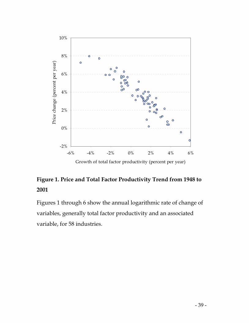
Figure 1 shows a scatter plot of the total factor productivity and

price trends over the 1948-2001 period. The negative association is clear.

Table 1 shows the battery of tests for price trends. The industries in each

segment are listed in Appendix A, while details on the estimation are

provided in Appendix B. In each case, we report the coefficient of a

regression of the variable listed (average annual logarithmic change in

price in this case) on a measure of the annual logarithmic change in

productivity.

These tests show that productivity trends are associated almost

percentage-point for percentage-point with price declines. The most

pertinent results here are for the well-measured industries; the

summary coefficient is -0.965. This coefficient is well determined and is

not significantly different from one.

The results here are very powerful. They indicate that the major

determinant of long-term relative price trends is relative productivity

trends. The main notable feature is that consumers capture virtually all

the gains from technological change.

Summary diagnosis 1. The hypothesis of a cost-price disease due

to slow productivity growth is strongly supported by the historical

data. Industries with relatively lower productivity growth show a

- 19 -

percentage-point for percentage-point higher growth in relative

prices.

2. Does Low Productivity Growth Lead to Stagnating Real

Output?

The next question is whether relatively slow productivity growth

leads to relatively slow real output growth. This would seems an

obvious point but in fact is not. If differential output growth is driven

primarily by demand shifts rather than supply shifts, it would be

possible that there would be little association between productivity

growth and output growth. Baumol states the hypothesis as follows:15

In the model of unbalanced productivity there is a tendency for

the outputs of the “nonprogressive” sector whose demands are not

highly inelastic to decline and perhaps, ultimately, to vanish....

We see then that costs in many sectors of the economy will rise

relentlessly, and will do so for reasons that are for all practical purposes

beyond the control of those involved. The consequence is that the

outputs of these sectors may in some cases tend to be driven from the

market.

The relationship between productivity growth and real output

growth was investigated in detail in an earlier section. That section


of Urban Crisis,” The American Economic Review, Vol. 57, No. 3, June, 1967,

pp. 418, 420.

- 20 -

showed that, under ideal circumstances, the cross section coefficient of

real output growth on TFP growth would be (the negative of) the

average elasticity of demand in the SAIDS system.

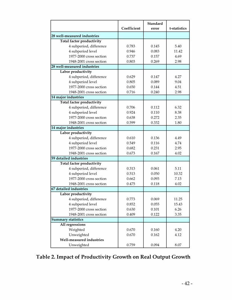
Figure 2 shows the growth of real output and in total factor

productivity (TFP) over the 1948-2001 period. There is a clear positive

relationship between TFP growth and output growth. Table 2 shows the

formal tests of the relationship between real output and productivity

growth. Looking across the different specifications, there is a very

strong positive association between productivity growth and real

output growth. Every single specification has a statistically significant

positive coefficient. The summary coefficients – measuring the elasticity

of real output with respect to productivity – are between 0.67 and 0.76,

and the coefficients are well determined. For the well-measured

industries, the relationship is very tight, with a one percentage-point

faster productivity growth leading to a 0.76 percentage-point higher

growth in real output.

Among industries with well-measured output, the five industries

with declining real output over the period, starting from the bottom, are

Tobacco products, Local and interurban passenger transit, Personal

households, Leather and leather products, and Miscellaneous repair

services. Each of these has a tale to tell. Tobacco, local transit, and

miscellaneous repair service had negative measured TFP growth over

the 1948-2001 period. Tobacco was probably driven to distraction by

regulation, and there are no reliable measures of productivity for

private households.

- 21 -

Looking at the five industries with the most rapidly rising real

output over the 1948-2001 period, starting from the top, we have

Transportation by air, Electronic and other electric equipment,

Telephone and telegraph, Trucking and warehousing, and Wholesale

trade. All five had very dynamic technologies, and all five had high TFP

growth over the period.

Summary diagnosis 2. The real output/stagnation hypothesis is

strongly confirmed. Technologically stagnant industries have shown

slower growth in real output than have the technologically dynamic

ones. A one percentage-point higher productivity growth was

associated with a three-quarters percentage-point higher real output

growth.

3. Do Industries With Slow Productivity Growth Have

Declining Nominal Output Shares?

For the most part, businesses care very little about their real

output growth. They care about dollar sales, profits, and employment.

What are those relationships? Baumol recognized that there were

different possible cases:16

16 William J. Baumol, “Macroeconomics of Unbalanced Growth: Comment (in

Communications),” The American Economic Review, Vol. 58, No. 4, Sept, 1968,

pp. 897.

- 22 -

Having predicted a cumulative cost rise for the output of the

“nonprogressive sector” of the economy I did not intend to go further

and attempt a generalized forecast of the activities that compose it. I

meant to suggest a variety of possibilities: that some, like the

construction of stately homes, would tend to disappear; that others,

such as very fine restaurants, would be reduced to a small number

catering almost exclusively to the very affluent; that some, like

handmade furniture and pottery, would fall into the hands of amateur

craftsmen; and that some, such as education (at least up to this point)

would continue to be demanded but would, as a consequence, eat up

an ever-growing portion of GNP. I do not believe that any one type of

time path will characterize the behavior of every output of the

nonprogressive sector in the future any more than it has until now.

In later work, Baumol, Blackman, and Wolff sharpened the view,

focusing primarily on services:17

The “rising share of services” turns out to be somewhat illusory.

The [real] output shares of the progressive and stagnant sectors have in

fact remained fairly constant in the postwar period, so that with rising

relative prices, the share of total expenditures on the (stagnant) services

and their share of the labor force have risen dramatically (their prices

rose at about the same rate as their productivity lagged behind the

progressive sectors), just as the model suggests. Similar trends are also

found internationally.

17 Op. cit., p. 815-816.

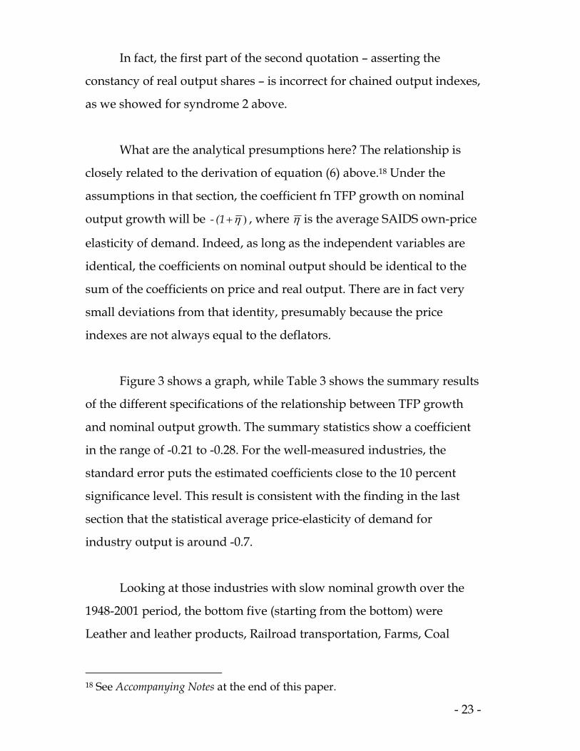
In fact, the first part of the second quotation – asserting the

constancy of real output shares – is incorrect for chained output indexes,

as we showed for syndrome 2 above.

What are the analytical presumptions here? The relationship is

closely related to the derivation of equation (6) above.18 Under the

assumptions in that section, the coefficient fn TFP growth on nominal

output growth will be )η+(1- , where η is the average SAIDS own-price

elasticity of demand. Indeed, as long as the independent variables are

identical, the coefficients on nominal output should be identical to the

sum of the coefficients on price and real output. There are in fact very

small deviations from that identity, presumably because the price

indexes are not always equal to the deflators.

Figure 3 shows a graph, while Table 3 shows the summary results

of the different specifications of the relationship between TFP growth

and nominal output growth. The summary statistics show a coefficient

in the range of -0.21 to -0.28. For the well-measured industries, the

standard error puts the estimated coefficients close to the 10 percent

significance level. This result is consistent with the finding in the last

section that the statistical average price-elasticity of demand for

industry output is around -0.7.

Looking at those industries with slow nominal growth over the

1948-2001 period, the bottom five (starting from the bottom) were

Leather and leather products, Railroad transportation, Farms, Coal

18 See Accompanying Notes at the end of this paper.

- 23 -

- 24 -

mining, and Textile mill products. All of these had quite robust

productivity growth. Their decline was probably driven largely by

income effects, substitute products, or competition from abroad, but the

rapid growth in productivity and decline in prices was insufficient to

offset other influences.

The most rapid growth in nominal GDP was found in Social

services, Business services, Radio and television, Transportation by air,

and Health services. With the exception of air, these had low measured

TFP growth, although there are serious questions about measurement in

most cases.

Summary diagnosis 3: There is a negative association of

productivity growth with the growth in nominal output. In other

words, stagnant industries tend to take a rising share of nominal

output; however, the relationship is only marginally statistically

significant.

4. Do Industries With Slow Productivity Growth Have

Declining Relative Employment and Hours?

Perhaps the most interesting question from a social perspective is

whether stagnant industries are gaining or losing shares of labor inputs

– either employment or hours. Baumol, Blackman, and Wolff concluded

that the stagnant service sector was demanding an increasing share of

labor inputs:19

19 Op. cit., p. 806.

As the model predicts, the U.S. labor force has been absorbed

predominantly by the stagnant subsector of the services rather than the

services as a whole.

The analysis of the impact of productivity on labor inputs is

similar to that of nominal share of output, with the resulting impact

ambiguous. The reduced-form estimates of the impact of total factor

productivity changes on employment are derived from those on output

but have one additional complication involving the derived demand for

labor inputs. Assume that firms in an industry are identical and

minimize costs. Further assume that the wages in each industry are

exogenous (determined by market power, unions, and other factors).

From the earlier analysis, we can derive the following reduced-form

equation for the growth of labor inputs:20

(7) mititit

*it βw-a)(1- m εη +++= ˆˆˆˆ it

where

) a(ε- aiti

eit

x2it

x1i

ait

zittt

mit εεεεεεε η +++++++= itaz ˆˆˆ

The major new twist here is the variable , the rate of change of

the elasticity of output with respect to labor. This represents biased

technological change in the Cobb-Douglas framework. The errors here

were defined above except for , which is the error in the equation for

demand for labor inputs.

itβ

eitε

20 See the Accompanying Notes at the end of this paper.

- 25 -

Equation (7) shows that the coefficient on TFP growth in the

employment equation is )η+− 1( , which is minus (one plus the average

price-elasticity of demand). This indicates that (holding other forces

constant) the growth of labor inputs such as employment or hours will

be positively or negatively affected by technological change depending

upon whether output demand is price-elastic or price-inelastic,

respectively. The trend will also be affected to the extent that there is

differential wage growth in the industry, or if there is biased

technological change (represented by the rate of growth of the output

elasticity, ). itβ

Figure 4 shows the association of hours growth and TFP growth.

The negative association – similar to that for nominal output and TFP

growth – is evident. Table 4 shows the battery of tests run on hours,

which indicates a negative association of hours and productivity. The

results are particularly strong for the 1977-2000 period for which the

data are most reliable; also, they are uniformly negative for the well-

measured industries. The average effect for well-measured industries

shows that a 1 percentage-point higher productivity growth is

associated with a 0.26 percentage-point lower growth in hours worked.

The results for employment are virtually identical, with the coefficients

and t-statistics very close to those for hours.

These results are consistent with those for nominal and real

output. They suggest that the most important factor driving differential

employment growth has been differential technological change across

industries. We can also test for the impacts of differential wage growth

- 26 -

- 27 -

and biased technological change by including the growth of wages and

the change in the share of compensation in the equations. For this

purpose, I concentrate only on the results for TFP growth for the

detailed industry groups. Adding either or both of wage growth or the

rate of growth of the labor share does not change the coefficient on total

factor productivity. It is interesting to note that the coefficient on biased

technological change is insignificant and very small. This result suggests

that, at least in these data, differential technological change was not

important in the relative demand for employment across different

sectors.

Differing Results for Manufacturing

One interesting extension of findings should be mentioned. The

results for manufacturing differ from those for the overall economy. A

careful examination of the impact of differential productivity growth on

employment and hours for detailed manufacturing industries finds a

positive rather than a negative relationship between productivity

growth and hours worked.21 The difference between manufacturing and

other industries probably arises because the openness of manufacturing

leads to more price-elastic demand for domestic production and

therefore to a positive relationship between productivity growth on the

one hand and nominal output and hours growth on the other hand.

Further research is needed in this area, but the difference between

21 William D. Nordhaus, “The Sources of the Productivity Rebound and the

Manufacturing Employment Puzzle,” NBER Working Paper No. 11354, May

2005.

- 28 -

manufacturing and the entire economy suggests the importance of

openness to the productivity-employment relationship.

Summary diagnosis 4: Industries with more rapid productivity

growth tend to displace labor and show lower growth of hours and

employment. However, this relationship appears to be reversed

within manufacturing industries, which show higher growth of labor

inputs with higher productivity growth.

5. Who Captures the Gains From Innovation?

A central question of economic growth concerns the distribution

of the fruits of productivity growth. Who captures the gains from

innovation, and who suffers losses from stagnation? The results on

pricing for syndrome 1 suggest that most of the gains are captured by

consumers in the form of lower prices. Are there any residual rewards

to either capital or labor? In their studies on the performing arts, Bowen

and Baumol argued that the low earnings and stressed financial status

in such industries were due to the stagnant productivity performance.22

Productivity and wages

22 William J. Baumol and William G. Bowen, “On the Performing Arts: The

Anatomy of their Economic Problems.” The American Economic Review, Vol. 55,

No. 2, 1965, pp. 495-502. Baumol has written to me that he has changed his

view of the relationship between low wages and stagnant productivity sectors

since the 1965 article was written and does not believe that stagnant sectors

necessarily show low wages (personal communication, October 28, 2004).

- 29 -

The general picture for wages is shown in Figure 5, which

indicates little relationship between productivity growth and wage

growth. Table 5 shows a battery of tests of the impact of relative

productivity growth on relative wages. Higher productivity growth has

a small positive impact on wage relative growth with an inconsistent

sign. For well-measured industries, the sign is slightly positive.

However, for all industries in the cross-section (shown in Figure 5), the

sign is negative, reflecting some strange outliers at the upper left. These

outliers are tobacco and several service industries, where output is

probably poorly measured.

In any case, the relative importance of productivity on differential

wages is very small. For example, the unweighted average effect across

different specifications is a 0.017 percent increase in wages per percent

increase in productivity. If we take the 0.017 coefficient and apply it to

the differences in productivity growth across industries, it would yield a

maximum wage differential of about 8 percent for the entire 1948-2001

period between the best and worst performer. This predicted impact

compares with the range of differential wage growth of 132 percent.

This result suggests that the low wages in the performing arts and other

stagnant sectors are due to factors other than productivity stagnation,

the most likely being a combination of compensating variations and a

winner-take-all incentive structure.

- 30 -

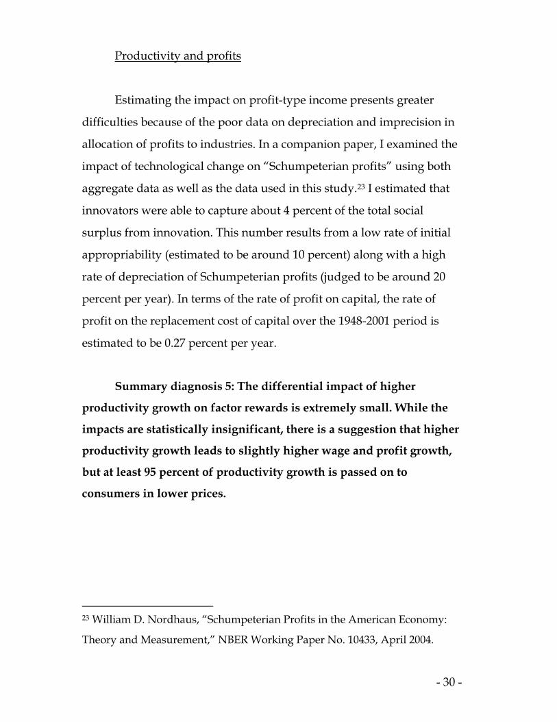
Productivity and profits

Estimating the impact on profit-type income presents greater

difficulties because of the poor data on depreciation and imprecision in

allocation of profits to industries. In a companion paper, I examined the

impact of technological change on “Schumpeterian profits” using both

aggregate data as well as the data used in this study.23 I estimated that

innovators were able to capture about 4 percent of the total social

surplus from innovation. This number results from a low rate of initial

appropriability (estimated to be around 10 percent) along with a high

rate of depreciation of Schumpeterian profits (judged to be around 20

percent per year). In terms of the rate of profit on capital, the rate of

profit on the replacement cost of capital over the 1948-2001 period is

estimated to be 0.27 percent per year.

Summary diagnosis 5: The differential impact of higher

productivity growth on factor rewards is extremely small. While the

impacts are statistically insignificant, there is a suggestion that higher

productivity growth leads to slightly higher wage and profit growth,

but at least 95 percent of productivity growth is passed on to

consumers in lower prices.

23 William D. Nordhaus, “Schumpeterian Profits in the American Economy:

Theory and Measurement,” NBER Working Paper No. 10433, April 2004.

- 31 -

6. Has the economy suffered from a growth disease?

A final and intriguing question is the impact of the changing

composition of output on overall productivity growth – a syndrome we

denote “Baumol’s growth disease.” Baumol’s growth disease occurs

when stagnant sectors (those with relatively slow productivity growth)

also have rising nominal output shares. The point can be seen by

comparing people with different tastes. Person A’s tastes run to

computers, software, and consumer electronics, while person B’s tend

toward New York real estate, Picasso paintings, and three-star Parisian

restaurants. Because person A’s consumption is tilted toward items

whose prices are falling rather than rising rapidly, A’s real income will

be experiencing a rapid increase relative to B’s real income associated

with Upper East Side tastes. Baumol’s discussion of this tendency was

the following:24

An attempt to achieve balanced growth in a world of unbalanced

productivity must lead to a declining rate of growth relative to the rate

of growth of the labor force. In particular, if productivity in one sector

and the total labor force remain constant the growth rate of the

economy will asymptotically approach zero.


of Urban Crisis,” The American Economic Review, Vol. 57, No. 3, June, 1967, pp.

419. Baumol commented that did not intend to say that the productivity

disease would slow growth; he views the disease as a cost disease, not a

growth disease (personal communication, October 28, 2004).

Analytics of the growth disease

The macroeconomics of the growth disease can be seen by

examining the growth of real output. Using the Törnqvist formula, real

output growth is equal to the weighted growth of output in different

sectors, where the weights are nominal shares of output. If stagnant

sectors have rising nominal output shares, then the aggregate growth

rate will be reduced as the share of output moves toward the slow

productivity-growth sectors.

This tendency can be seen by decomposing aggregate

productivity growth.25 Define as aggregate productivity growth and

as the growth of aggregate inputs. The one-period growth rate of TFP

is:

ta

tb

(8) ∑ ∑= =

−=−=n

1i

n

1iititititttt V b S xbxa ˆˆˆˆˆ

- 32 -

25 This derivation relies on value-added superlative production relationships.

An alternative approach is used in Kevin Stiroh, “Information Technology and

U.S. Productivity Revival: What Do the Industry Data Say?” American

Economic Review, vol. 92, no. 5, pp. 1559-76. The decomposition for total output

is found in Dale W. Jorgenson, Frank W. Gollop, and Barbara M. Fraumeni,

Productivity and U.S. Economic Growth, Harvard University Press, Cambridge,

MA, 1987. One advantage of the decomposition used here is that the

redistribution effects are much smaller than those using total output and

Domar weights.

Here, = the Törnqvist share of inputs of industry i in

the total. Add and subtract to (6) and reorganize:

⎟⎟⎠

⎞⎜⎜⎝

⎛= ∑

=

n

1jtjtiit B / B V

∑=

n

1iitit S b

(9) ∑∑==

−+=n

1iititit

n

1iititt )(S b S aa Vˆˆˆ

The two terms on the right-hand side of (9) are a pure productivity term

and a redistribution effect. The pure productivity term measures the

aggregate growth rate as the weighted sum of industrial growth rates.

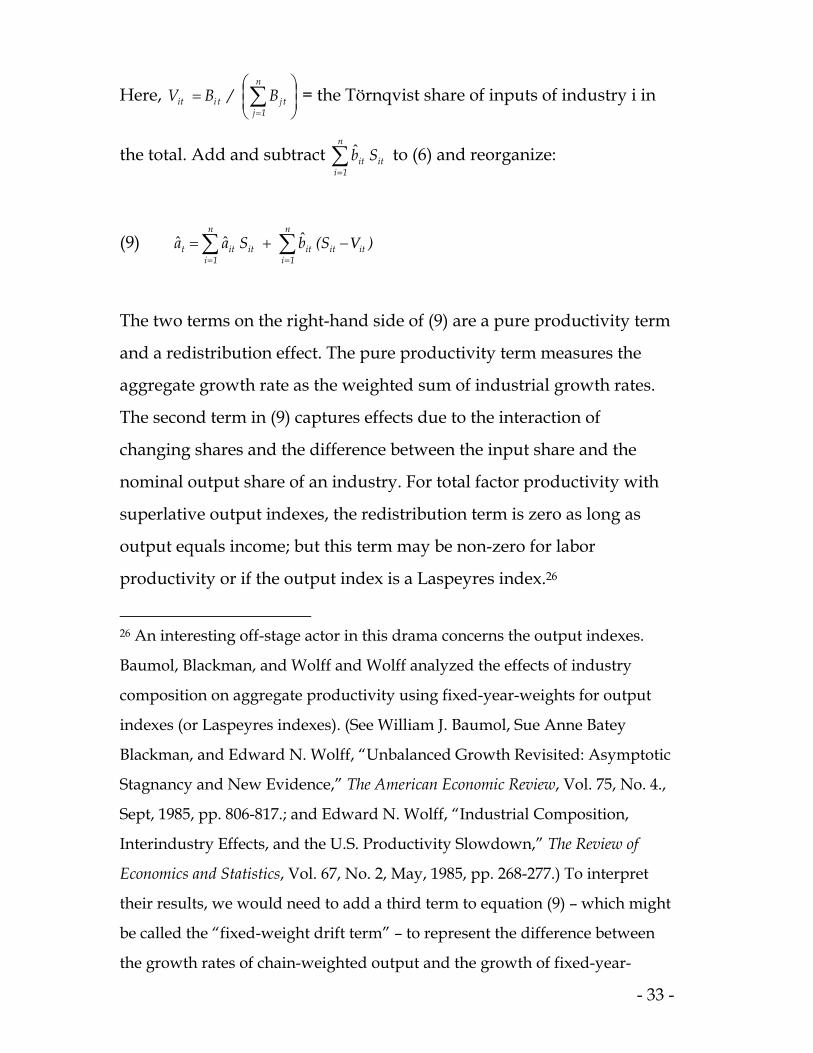
The second term in (9) captures effects due to the interaction of

changing shares and the difference between the input share and the

nominal output share of an industry. For total factor productivity with

superlative output indexes, the redistribution term is zero as long as

output equals income; but this term may be non-zero for labor

productivity or if the output index is a Laspeyres index.26

- 33 -

26 An interesting off-stage actor in this drama concerns the output indexes.

Baumol, Blackman, and Wolff and Wolff analyzed the effects of industry

composition on aggregate productivity using fixed-year-weights for output

indexes (or Laspeyres indexes). (See William J. Baumol, Sue Anne Batey

Blackman, and Edward N. Wolff, “Unbalanced Growth Revisited: Asymptotic

Stagnancy and New Evidence,” The American Economic Review, Vol. 75, No. 4.,

Sept, 1985, pp. 806-817.; and Edward N. Wolff, “Industrial Composition,

Interindustry Effects, and the U.S. Productivity Slowdown,” The Review of

Economics and Statistics, Vol. 67, No. 2, May, 1985, pp. 268-277.) To interpret

their results, we would need to add a third term to equation (9) – which might

be called the “fixed-weight drift term” – to represent the difference between

the growth rates of chain-weighted output and the growth of fixed-year-

To measure the Baumol growth effect, we estimate the growth

rate using nominal output shares for a given year, T, and denote the

results as the “fixed-shares growth rate” or “FSGR(T)”:

(10) FSGR(T) = ∑ =

n

1iiTit S a

By comparing the FSGR(T) for different base years, we can determine

the impact of changing output shares on the growth of productivity. If

the FSGR is lower for later T, then the Baumol growth effect is negative,

indicating that shares are moving in a manner that is unfavorable to

growth. If the FSGR is higher for later T, then the Baumol growth effect

is positive.

Results

Figure 6 and Table 6 show the FSGR for aggregate total factor

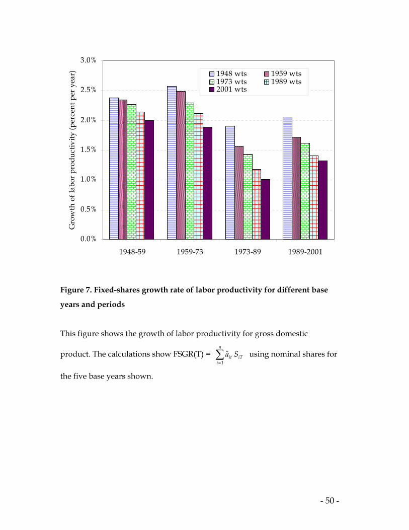
productivity, and Figure 7 shows the results for aggregate labor

productivity. To get a flavor of the results, examine the last line in Table

6. This shows the aggregate rate of growth of total factor productivity

for 1948-2001 where the industries are weighted with nominal output

shares for five different years. If we use fixed shares for 1948, the

average rate of TFP growth would be 1.49 percent per year, whereas if

- 34 -

weighted output. The fixed-weight drift term exited the stage when old-style

Laspeyres indexes were replaced by superlative indexes, and it will not

feature in the discussion here.

- 35 -

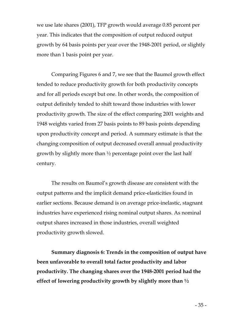
we use late shares (2001), TFP growth would average 0.85 percent per

year. This indicates that the composition of output reduced output

growth by 64 basis points per year over the 1948-2001 period, or slightly

more than 1 basis point per year.

Comparing Figures 6 and 7, we see that the Baumol growth effect

tended to reduce productivity growth for both productivity concepts

and for all periods except but one. In other words, the composition of

output definitely tended to shift toward those industries with lower

productivity growth. The size of the effect comparing 2001 weights and

1948 weights varied from 27 basis points to 89 basis points depending

upon productivity concept and period. A summary estimate is that the

changing composition of output decreased overall annual productivity

growth by slightly more than ½ percentage point over the last half

century.

The results on Baumol’s growth disease are consistent with the

output patterns and the implicit demand price-elasticities found in

earlier sections. Because demand is on average price-inelastic, stagnant

industries have experienced rising nominal output shares. As nominal

output shares increased in those industries, overall weighted

productivity growth slowed.

Summary diagnosis 6: Trends in the composition of output have

been unfavorable to overall total factor productivity and labor

productivity. The changing shares over the 1948-2001 period had the

effect of lowering productivity growth by slightly more than ½

- 36 -

percentage point per year, indicating that Baumol’s growth disease

was an important factor during this period.

V. Conclusions

The present study has investigated a series of hypotheses

concerning the effects of productivity change on economic growth,

prices, and factor rewards. Before summarizing, two reservations must

be noted. First, the results presented here rely upon data on value-

added prices, output, and productivity by industry, such as

entertainment and textiles. These data are not completely adequate for

questions concerning final goods and services such as concerts or

clothing. For most cases, they are close but imperfect substitutes for the

ideal data.

Second, the data are sometimes poorly measured estimates of true

output and therefore cannot correctly calculate true prices or the correct

numerator for productivity. This shortcoming is particularly serious in

services such as health, education, and personal services, for which the

output measures are in reality measures of inputs. We have dealt with

measurement issues by taking different slices of the data, such as

examining data for different periods or for subsets of industries that are

well-measured, but we cannot wholly overcome the mismeasurement

difficulties.

Subject to these reservations, the results here speak clearly on

many of the hypotheses put forth by Baumol and his co-authors. The

data are particularly useful because they are a comprehensive account

- 37 -

of the market economy of the United States for more than a half-

century. Here are the major results.

First, Baumol’s hypothesis of a cost-price disease due to slow

productivity growth is definitely confirmed by the data. Industries with

relatively low productivity growth (“stagnant industries”) show a

percentage-point for percentage-point higher growth in relative prices.

This result indicates that most of the economic gains from higher

productivity growth are passed on to consumers in lower prices.

Moreover, differences in productivity over the long term of a half-

century explain around 85 percent of the variance in relative price

movements for well-measured industries. While the underlying forces

driving technological change remain a challenge, the impacts of

differential technological change on prices stand out clearly.

Second, the real output stagnation hypothesis is strongly

confirmed. Industries that are technologically stagnant tend to have

slower growth in real output than do the technologically dynamic ones,

with a one percentage-point lower productivity growth being associated

with a three-quarters percentage-point lower real output growth.

Moreover, the statistical association of output growth and productivity

growth is highly significant. The mechanism by which productivity

affects output is clearly through the price mechanism of the cost-price

disease.

Third, beyond the price and real output effects, the associations

become murkier. One interesting question is how higher industrial

productivity growth affects jobs. Industries with higher productivity

- 38 -

growth generally had declining employment and hours growth when

all industries are considered. However, this relationship was reversed

for internationally open manufacturing sectors.

Fourth, the differential impact of higher productivity growth on

factor rewards is extremely small. There is a suggestion that higher

industrial productivity growth leads to slightly higher industrial wage

growth and to higher profits, but the fraction of productivity retained as

higher factor rewards is very small. For the most part, industrial wage

and profit trends are determined by the aggregate economy and not by

the productivity experience of individual sectors.

Perhaps the most important macroeconomic result is the

operation of Baumol’s growth disease over the last half of the twentieth

century. The hypothesis underlying the growth disease is that – because

the composition of output has shifted away from industries with rapid

productivity growth like manufacturing toward those with stagnant

technologies like government, education, and construction – aggregate

productivity growth has slowed. There has indeed been a tendency for

changes in spending shares to slow economic growth. The growth

disease has lowered annual aggregate productivity growth by slightly

more than one-half percentage point over the last half century.

-2%

0%

2%

4%

6%

8%

10%

-6% -4% -2% 0% 2% 4% 6

Growth of total factor productivity (percent per year)

Pric

e ch

ange

(per

cent

per

yea

r)

%

Figure 1. Price and Total Factor Productivity Trend from 1948 to

2001

Figures 1 through 6 show the annual logarithmic rate of change of

variables, generally total factor productivity and an associated

variable, for 58 industries.

- 39 -

CoefficientStandard

error t-statisticsObserv-ations

28 well-measured industriesTotal factor productivity

4 subperiod, difference -1.232 0.153 -8.06 844 subperiod level -0.887 0.079 -11.17 1121977-2000 cross section -0.972 0.070 -13.90 281948-2001 cross section -0.968 0.088 -11.03 28

28 well-measured industriesLabor productivity


14 major industriesTotal factor productivity


14 major industriesLabor productivity


59 detailed industriesTotal factor productivity


67 detailed industriesLabor productivity


Summary statisticsAll regressions

Weighted -0.956 0.129 -7.38Unweighted -0.942 0.167 -5.66

Well-measured industriesUnweighted -0.965 0.131 -7.38

Table 1. Impact of Productivity Growth on Price Change

(For a discussion of the specification and variables, see

Appendix B.)

- 40 -

-4%

-2%

0%

2%

4%

6%

8%

10%

-6% -4% -2% 0% 2% 4% 6% 8%

Growth of total factor productivity

Real

out

put g

row

th

Figure 2. TFP Growth and Real Output Growth, 1948-2001

(annual average percent per year)

- 41 -

CoefficientStandard

error t-statistics


4 subperiod, difference 0.783 0.145 5.404 subperiod level 0.946 0.083 11.421977-2000 cross section 0.737 0.157 4.691948-2001 cross section 0.803 0.269 2.98












Weighted 0.670 0.160 4.20Unweighted 0.670 0.162 4.12

Well-measured industriesUnweighted 0.759 0.094 8.07

Table 2. Impact of Productivity Growth on Real Output Growth

- 42 -

0%

2%

4%

6%

8%

10%

12%

-6% -4% -2% 0% 2% 4% 6% 8%


Nom

inal

out

put g

row

th

Figure 3. Growth of TFP and nominal output, 1948-2001 (annual

average percent per year)

- 43 -

CoefficientStandard

error t-statisticsSummary statistics

All regressionsWeighted -0.276 0.198 -1.39Unweighted -0.272 0.195 -1.40


Table 3. Impact of productivity growth on nominal output

growth

Note: the coefficients of nominal output growth are very close to the

sum of the coefficients of price plus real output growth (see text)

- 44 -

-6%

-4%

-2%

0%

2%

4%

6%

8%

-6% -4% -2% 0% 2% 4% 6% 8%

Growth of total factor productivity (percent per year)

Hou

rs c

hang

e (p

erce

nt p

er y

ear)

Figure 4. Growth of TFP and hours, 1948-2001

- 45 -

CoefficientStandard

error t-statistics


4 subperiod, difference -0.206 0.162 -1.274 subperiod level -0.066 0.097 -0.681977-2000 cross section -0.351 0.163 -2.151948-2001 cross section -0.248 0.272 -0.91




4 subperiod, difference -0.102 0.135 -0.764 subperiod level 0.121 0.146 0.831977-2000 cross section -0.311 0.324 -0.961948-2001 cross section -0.459 0.351 -1.31




4 subperiod, difference 0.053 0.050 1.064 subperiod level 0.097 0.041 2.351977-2000 cross section -0.253 0.103 -2.471948-2001 cross section -0.453 0.128 -3.53




Weighted -0.282 0.150 -1.87Unweighted -0.258 0.193 -1.34


Table 4. Impact of productivity growth on hours growth

- 46 -

4.5%

5.0%

5.5%

6.0%

6.5%

7.0%

7.5%

-6% -4% -2% 0% 2% 4% 6% 8%


Wag

e ra

te g

row

th

Figure 5. Productivity growth and wage growth by

industry, 1948-2001 (annual average percent per year)

- 47 -

Coefficient Standard error t-statistics28 well-measured industries

Total factor productivity4 subperiod, difference -0.082 0.064 -1.284 subperiod level 0.086 0.045 1.901977-2000 cross section 0.086 0.058 1.471948-2001 cross section 0.079 0.054 1.46


4 subperiod, difference -0.022 0.062 -0.364 subperiod level 0.105 0.042 2.501977-2000 cross section 0.109 0.050 2.161948-2001 cross section 0.115 0.045 2.55


4 subperiod, difference -0.135 0.105 -1.284 subperiod level 0.065 0.088 0.751977-2000 cross section -0.018 0.180 -0.101948-2001 cross section 0.004 0.130 0.03




4 subperiod, difference 0.026 0.024 1.104 subperiod level -0.005 0.021 -0.241977-2000 cross section -0.088 0.037 -2.361948-2001 cross section -0.052 0.031 -1.66


4 subperiod, difference 0.018 0.036 0.494 subperiod level 0.076 0.028 2.741977-2000 cross section -0.056 0.039 -1.431948-2001 cross section -0.029 0.031 -0.94


Weighted -0.001 0.078 -0.02Unweighted 0.017 0.074 0.23

Well-measured industriesUnweighted 0.059 0.067 0.88

Table 5. Coefficient of wage growth on productivity growth,

alternative specifications

- 48 -

0.0%

0.5%

1.0%

1.5%

2.0%

1948-59 1959-73 1973-89 1989-2001

TFP

grow

th (%

per

yea

r)

1948 wts 1959 wts1973 wts 1989 wts2001 wts

Figure 6. Fixed-shares growth rate of total factor productivity for different

base years and periods

This figure shows the fixed-shares growth rate of total factor productivity for

the aggregate of BEA industries for which capital stocks are available. These

comprised 83 percent of GDP in 2001. The calculations show FSGR(T) =

using fixed nominal shares for the five periods shown. The declining

rates show that the Baumol growth disease had a major impact on overall

productivity growth during this period.

∑=

n

1iiTit S a

- 49 -

0.0%

0.5%

1.0%

1.5%

2.0%

2.5%

3.0%

1948-59 1959-73 1973-89 1989-2001

Gro

wth

of l

abor

pro

duct

ivity

(per

cent

per

yea

r) 1948 wts 1959 wts1973 wts 1989 wts2001 wts

Figure 7. Fixed-shares growth rate of labor productivity for different base

years and periods

This figure shows the growth of labor productivity for gross domestic

product. The calculations show FSGR(T) = using nominal shares for

the five base years shown.

∑=

n

1iiTit S a

- 50 -

Productivity Fixed output-share weights for period Current growth for: 1948 1959 1973 1989 2001 weights

[percent per year, logarithmic growth]1948-59 1.61 1.75 1.71 1.51 1.34 1.641959-73 1.44 1.39 1.26 1.03 0.78 1.321973-89 1.27 0.92 0.83 0.56 0.38 0.591989-2001 1.73 1.47 1.42 1.19 1.11 1.13

1948-2001 1.49 1.34 1.26 1.02 0.85 1.12

Table 6. Fixed-shares growth rate for total factor productivity for different

weights and periods

Table shows the fixed-share growth rates, FSGR(T) = ∑ , for total factor

productivity, for different base years. The last column shows the current-year

(Törnqvist) growth in TFP. For the entire period, the annual average

difference between 1948 weights and 2001 weights is 0.64 percentage points.

=

n

1iiTit S a

- 51 -

- 52 -

Appendix A. Industry definitions in regressions

Industry definitions correspond to the 1987 SIC industry

code. Included industries in the different samples are as follow.

All 67 detailed industries

(Asterisks denote industries that do not have total factor productivity

estimates because BEA does not publish capital stock data.)

Farms

Agricultural services, forestry, and fishing

Metal mining

Coal mining

Oil and gas extraction

Nonmetallic minerals, except fuels

Construction

Lumber and wood products

Furniture and fixtures

Stone, clay, and glass products

Primary metal industries

Fabricated metal products

Industrial machinery and equipment

Electronic and other electric equipment

Motor vehicles and equipment

Other transportation equipment

Instruments and related products

Miscellaneous manufacturing industries

Food and kindred products

Tobacco products

Textile mill products

- 53 -

Apparel and other textile products

Paper and allied products

Printing and publishing

Chemicals and allied products

Petroleum and coal products

Rubber and miscellaneous plastics products

Leather and leather products

Railroad transportation

Local and interurban passenger transit

Trucking and warehousing

Water transportation

Transportation by air

Pipelines, except natural gas

Transportation services

Telephone and telegraph

Radio and television

Electric, gas, and sanitary services

Wholesale trade

Retail trade

Depository institutions

Nondepository institutions

Security and commodity brokers

Insurance carriers

Insurance agents, brokers, and service

Nonfarm housing services

Other real estate

Holding and other investment offices

Hotels and other lodging places

Personal services

Business services

Auto repair, services, and parking

Miscellaneous repair services

Motion pictures

- 54 -

Amusement and recreation services

Health services

Legal services

Educational services

Social services*

Membership organizations*

Other services*

Private households*

Federal general government*

Federal government enterprises*

State and local general government*

State and local government enterprises*

All 28 Well-Measured Industries

Farms

Metal mining

Coal mining

Nonmetallic minerals, except fuels

Lumber and wood products

Furniture and fixtures

Stone, clay, and glass products

Primary metal industries

Fabricated metal products

Industrial machinery and equipment

Electronic and other electric equipment

Motor vehicles and equipment

Other transportation equipment

Food and kindred products

Textile mill products

Apparel and other textile products

Paper and allied products

Printing and publishing

- 55 -

Chemicals and allied products

Rubber and miscellaneous plastics products

Leather and leather products

Railroad transportation

Trucking and warehousing

Transportation by air

Telephone and telegraph


Wholesale trade

Retail trade

One-Digit Industries

Farms

Mining

Construction

Durable goods

Nondurable goods

Transportation

Communications


Wholesale trade

Retail trade

Finance, insurance, and real estate

Services

Federal government

State and local governments

Appendix B. Notes on the Estimates in Tables 1 to 6

Details of Estimation for Tables 1 through 5

The results in Tables 1 through 5 were estimated using twenty-

four different specifications. One set uses two different measures of

productivity (labor productivity and total factor productivity). A second

set is three different industry combinations as described in Appendix A.

A third specification involves four different time periods.

The specifications for the different time periods will be described

in this Appendix. The first two equations in each block are panel

estimators with fixed effects, while the last two are cross-sections over

long timer periods.

As an example, the panel estimate in the second equation of Table

1 is:

(B-1) pitt210iit p εγγγ +++= Dait

*ˆˆ

where is the average annual change in the logarithm of price

between year 1948 and 1959 for t = 1, 1959 and 1973 for t = 2, 1973 and

1989 for t = 3, and 1989 and 2001 for t = 4. is the average annual

change in the logarithm of calculated industry productivity over the

same periods, Dt is a panel of time effects for the different periods, is

a random disturbance, the

itp

ita

pitε

0iγ are industry effects, while 1γ and 2γ are

coefficients. The first equation in each block takes the first difference of

- 56 -

- 57 -

equation in (B-1). The last two sets of equations are cross sections for

either the shorter period for which the data are better or for the entire

period. The equations are estimated using the panel estimator and

ordinary least squares in Eviews 5.0.

The summary statistics at the bottom of each table are calculated

under the assumption that each equation is independent. While this

assumption is clearly not the case, it is a convenient way of organizing

the different results. The weighted summary statistics take the estimates

shown in the columns above it and weight the coefficients by the

number of observations for each equation. The unweighted statistics

weight each equation equally.

Documents

Baumol’s Cost Disease: A Macroeconomic Perspective · Baumol’s Diseases: A Macroeconomic Perspective William D. Nordhaus NBER Working Paper No. 12218 May 2006 JEL No. D4, O3,