Embed Size (px)
Citation preview

2
Graph = Network
• G(V, E): graph (network)
V: vertices (nodes), E: edges (links)
1
2 3
4
5
Nodes = 1, 2, 3, 4, 5
Links = 1<->2, 1<->3, 1<->5, 2<->3, 2<->4, 2<->5, 3<->4, 3<->5, 4<->5 (Nodes may have states; links may have directions and weights)

3
Representation of a network
• Adjacency matrix:
A matrix with rows and columns labeled by nodes, where element aij shows the number of links going from node i to node j
(becomes symmetric for undirected graph)
• Adjacency list:
A list of links whose element “i->j” shows a link going from node i to node j
(also represented as “i -> {j1, j2, j3, …}”)

4
Exercise
• Represent the following network in:
– Adjacency matrix
– Adjacency list
1
2 3
4
5
5
Degree of a node
u1 u2
• A degree of node u, deg(u), is the number of links connected to u
deg(u1) = 4 deg(u2) = 2

6
Connected graph
• A graph in which there is a path between any pair of nodes

7
Number of connected components
= 2
Connected component
Connected component
Connected components

8
Complete graph
• A graph in which any pair of nodes are connected (often written as K1, K2, …)

9
Regular graph
• A graph in which all nodes have the same degree (often called k-regular graph with degree k)
10
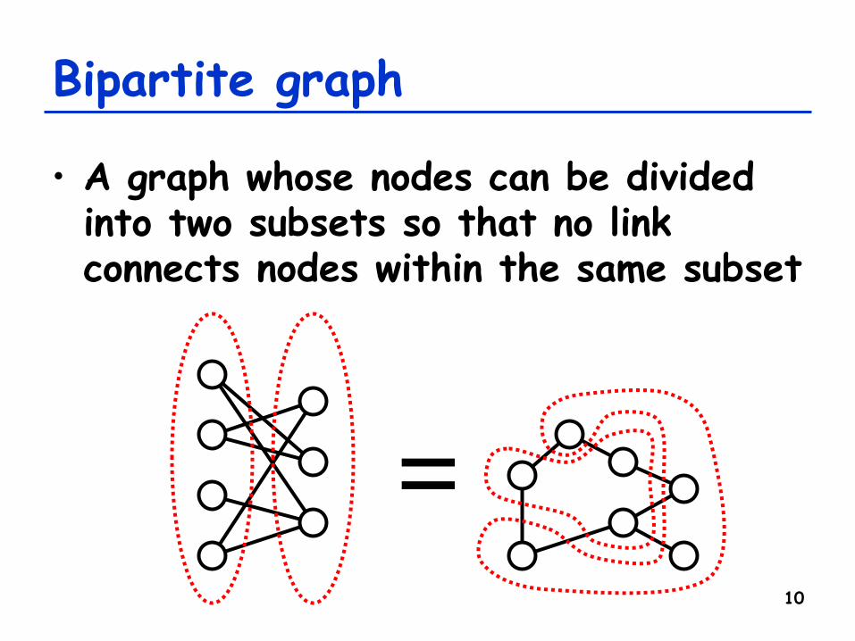
Bipartite graph
• A graph whose nodes can be divided into two subsets so that no link connects nodes within the same subset
=

11
Directed graph
• Each link is directed
• Direction repre-sents either order of relationship or accessibility between nodes
E.g. genealogy

12
Weighted directed graph
• Most general version of graphs
• Both weight and direction is assigned to each link
E.g. traffic network

Measuring Topological Properties of Networks (1):
Macroscopic Properties

Network density
• The ratio of # of actual links and # of possible links
– For an undirected graph:
d = |E| / ( |V| (|V| - 1) / 2 )
– For a directed graph:
d = |E| / ( |V| (|V| - 1) )
14

15
Characteristic path length
• In graph theory: Maximum of shortest path lengths between pairs of nodes (a.k.a. network diameter)
• In complex network science: Average shortest path lengths
• Characterizes how large the world being modeled is – A small length implies that the network is well connected globally

16
Clustering coefficient
• For each node: – Let n be the number of its neighbor nodes
– Let m be the number of links among the k neighbors
– Calculate c = m / (n choose 2)
Then C = <c> (the average of c)
• C indicates the average probability for two of one’s friends to be friends too – A large C implies that the network is well connected locally to form a cluster

17
Degree distribution
P(k) = Prob. (or #) of nodes with degree k
• Gives a rough profile of how the connectivity is distributed within the network
Sk P(k) = 1 (or total # of nodes)

18
Power law degree distribution
• P(k) ~ k-g
Scale-free network k
P(k)
log k
log P(k)
Linear in log-log plot
-> No characteristic scale (Scale-free networks)
A few well-connected nodes, a lot of poorly connected nodes

19
How it appears
Random Scale-free

Degree Distributions of Real-World Complex Networks
20
A Barabási, R Albert Science 1999;286:509-512
Actors WWW Power grid

Degree distribution of FB
21
• http://www.facebook.com/note.php?note_id=10150388519243859
• http://arxiv.org/abs/1111.4503
P(k) CCDF

Measuring Topological Properties of Networks (2): Centralities

23
Centrality measures (“B,C,D,E”)
• Degree centrality – How many connections the node has
• Betweenness centrality – How many shortest paths go through the node
• Closeness centrality – How close the node is to other nodes
• Eigenvector centrality

Degree centrality
• Simply, # of links attached to a node
CD(v) = deg(v)
or sometimes defined as
CD(v) = deg(v) / (N-1)
24

Betweenness centrality
• Prob. for a node to be on shortest paths between two other nodes
CB(v) = Σs≠v,t≠v • s: start node, e: end node
• #sp(s,e,v): # of shortest paths from s to e that go though node v
• #sp(s,e): total # of shortest paths from s to e
• Easily generalizable to “group betweenness” 25
#sp(s,e,v)
#sp(s,e)

Closeness centrality
• Inverse of an average distance from a node to all the other nodes
CC(v) =
• d(v,w): length of the shortest path from v to w
• Its inverse is called “farness”
• Sometimes “Σ” is moved out of the fraction (it works for networks that are not strongly connected)
• NetworkX calculates closeness within each connected component
26
n-1
Σw≠v d(v,w)

Eigenvector centrality
• Eigenvector of the largest eigenvalue of the adjacency matrix of a network
CE(v) = (v-th element of x)
Ax = lx
• l: dominant eigenvalue
• x is often normalized (|x| = 1)
27

Exercise
• Who is most central by degree, betweenness, closeness, eigenvector?
28

Which centrality to use?
• To find the most popular person
• To find the most efficient person to collect information from the entire organization
• To find the most powerful person to control information flow within an organization
• To find the most important person (?)
29

Measuring Topological Properties of Networks (3):
Mesoscopic Properties

Degree correlation (assortativity)
• Pearson’s correlation coefficient of node degrees across links
r =
• X: degree of start node (in / out)
• Y: degree of end node (in / out)
31
Cov(X, Y)
σX σY

Assortative/disassortative networks
32 (from Newman, M. E. J., Phys. Rev. Lett. 89: 208701, 2002)
Social networks are assortative
Engineered / biological networks are disassortative

K-cores
• A connected component of a network obtained by repeatedly deleting all the nodes whose degree is less than k until no more such nodes exist – Helps identify where the core cluster is
– All nodes of a k-core have at least degree k
– The largest value of k for which a k-core exists is called “degeneracy” of the network
33

Exercise
• Find the k-core (with the largest k) of the following network
34

Coreness (core number)
• A node’s coreness (core number) is c if it belongs to a c-core but not (c+1)-core
• Indicates how strongly the node is connected to the network
• Classifies nodes into several layers – Useful for visualization
35

Community
• A subgraph of a network within which nodes are connected to each other more densely than to the outside – Still defined vaguely…
– Various detection algorithms proposed • K-clique percolation
• Hierarchical clustering
• Girvan-Newman algorithm
• Modularity maximization (e.g., Louvain method) 36 (diagram from Wikipedia)

Modularity
• A quantity that characterizes how good a given community structure is in dividing the network
Q =
• |Ein|: # of links connecting nodes that belong to the same community
• |Ein-R|: Estimated |Ein| if links were random 37
|Ein|-|Ein-R|
|E|

Community detection based on modularity
• The Louvain method – Heuristic algorithm to construct communities that optimize modularity • Blondel et al. J. Stat. Mech. 2008 (10): P10008
• Python implementation by Thomas Aynaud available at: – https://bitbucket.org/taynaud/python-louvain/
38