Embed Size (px)
Citation preview

BASICS OF HEAVY DUTY DIESEL NVH
November 7, 2006
Ed Green
Roush Industries, Inc.
734-779-7421, [email protected]

2
Course Outline
I. Introduction (8:00 AM - 8:15 AM) Roush Industries Ed Green Course objectives Pre-Quiz
II. Fundamentals of noise and vibration (N&V) (8:15 AM – 11:30 AM)A. Time and frequency domain analysis (8:15 AM – 8:45 AM)B. The single degree of freedom system (SDOF) (8:45 AM – 9:30 AM)C. Transmissibility and isolation (10:00 AM – 10:45 AM)D. The source/path/receiver model (10:45 AM – 11:00 AM)E. Summary (11:00 AM – 11:05 AM)F. Discussion (11:05 AM – 11:30 AM)
III. Vibration (12:30 PM – 3:00 PM)A. Sensitivity to vibration (12:30 PM – 12:45 PM)B. Forced vs resonant vibration (12:45 PM – 12:50 PM) C. Rotating machinery vibration, orders, and critical speed (12:50 PM – 1:00 PM)D. Vehicle driveline issues (1:00 PM – 2:00 PM)E. Summary (2:30 PM – 2:35 PM)F. Discussion (2:35 PM – 3:00 PM)
IV. Sound and sound quality (3:00 PM – 3:30 PM)A. Decibels and A-weighting (3:00 PM – 3:05 PM)B. Beating, fluctuation, roughness, loudness, sharpness, and knock (3:05 PM – 3:20 PM)C. Passby noise procedure and stationary noise requirement (3:20 PM – 3:30 PM)
V. N&V features of DDC engines (3:30 PM – 3:45 PM)A. Engine mounting systemB. Isolated oil panC. Isolated rocker coverD. Crankshaft damperE. Lined bellows exhaust manifold
VI. N&V sensors (3:45 PM – 4:00 PM)A. AccelerometersB. MicrophonesC. Rotational speed transducersD. Transducer calibration
• Quiz and Review (4:00-4:30)

3
I. Introduction
Roush Industries Detroit based automotive engineering service company. Associated with famous Roush NASCAR Racing Teams. 2200 employees total. 45 employees dedicated to noise and vibration engineering and
products. www.roushind.com

4
I. Introduction Ed Green
Ph.D. from Purdue University 1983-1984, earthquake certification of lightning
arrestors 1986-1990, modeling of ultrasonic sound waves for
NRC, ultrasonic inspection 1994-present, automotive N&V at Roush
Vehicle N&V engineering Noise-control-material engineering Vibration dampers Intake and exhaust systems Passby noise
Station ClassLightning Arrestor
5
I. Introduction
Course Objectives Give tools and training to improve efficiency of N&V issue field
response Provide an introduction to N&V concepts Teach “language” of N&V
Not to make experts

6
Pre-Quiz


8
II. Fundamentals of Noise and Vibration (N&V)
A. Time and frequency domain analysis
B. The single degree of freedom system (SDOF)
C. Transmissibility and isolation
D. The source/path/receiver model
E. Summary
F. Discussion

9
II.A. Time and Frequency Domain Analysis
Microphones and accelerometers produce time domain signals
The Fast Fourier Transform (FFT) is a technique used for conversion to the frequency domain (for display by spectrum analyzers like the MTS4100)

10
II.A. Time and Frequency Domain Analysis
With the FFT: Any time domain signal can be
approximated by a summation of sinusoids
A unique set of sinusoids is defined by magnitude, phase, and frequency (MTS4100 displays only magnitude vs frequency)
The magnitude vs frequency is called the “Spectrum”
Based on the frequency range, the MTS automatically filters the data and sets the sample rate.

11
II.A. Time and Frequency Domain Analysis Animation of FFT applied to a square wave.

12
II.A. Time and Frequency Domain Analysis
Animation of FFT applied to idle noise signal from a Series 60 engine.
Click to play sound

13
II.A. Time and Frequency Domain AnalysisAbout the Fast Fourier Transform – The Fourier Transform is a mathematical function that finds the best least squares fit of a function to a set of basis functions based on the sine and cosine functions.
The Fourier Transform is named for the French Mathematician and Physicist, Jean Baptiste Joseph (1768-1830).
The Fourier Transform (http://mathworld.wolfram.com/FourierTransform.html) is used to find the spectral terms of a closed form expression (such as, y(t) = cos(at2+bt+c)).
The Discrete Fourier Transform (DFT) (http://mathworld.wolfram.com/DiscreteFourierTransform.html) is used to calculate the spectral terms of a digitized signal.
The Fast Fourier Transform (FFT) (http://mathworld.wolfram.com/FastFourierTransform.html) is a specialized implementation of the DFT that requires that the set of digitized data have a radix-two length (i.e. 512, 1024, 2048, etc.). The FFT is much faster than the DFT, and the FFT is by far the most common implementation of the Fourier Transform.
The FFT was first published by Cooley and Tukey (J.W. Cooley and O.W. Tukey, “An Algorithm for the Machine Calculation of Complex Fourier Series,” Math. Comput. 19, 297-301, 1965).

14
II.A. Time and Frequency Domain Analysis
FFT Signal Processing Issues - For the task at hand (using the MTS 4100 to diagnose N&V field issues), an advanced knowledge of the FFT is not necessary, but some participants may be interested.
When signals are digitized, issues arise. These are aliasing, leakage, and quantization error.
Aliasing – The first step in calculating the FFT is to digitize the signal as shown in the figure. The signal is sampled at intervals of t. The sample frequency is defined as 1/t. The signal is digiitized by the A/D (analog to digital) circuit of the MTS 4100. If a signal entered the A/D circuit that had a frequency much faster than the sample frequency as shown in the figure, the digiitzed signal would have a lower frequency than the actual frequency as shown. This is called aliasing because a line appears in the spectrum that is not at the true frequency. To prevent aliasing, the sample frequency must be at least two times faster than the signal frequency. Put another way, the “Nyquist frequency” (equal to half the sample frequency) must be greater than the signal frequency.
To prevent aliasing, powerful, analog, low-pass filters called “anti-aliasing filters” or “brick-wall filters,” are applied to the analog signal before the A/D circuit. Anti-aliasing is automatically performed by the MTS 4100. Note that anti-aliasing filters must be analog filters and that aliased data cannot be repaired.
Digitized Signal
Example of Aliasing
15
II.A. Time and Frequency Domain Analysis
FFT Signal Processing Issues – Cont.
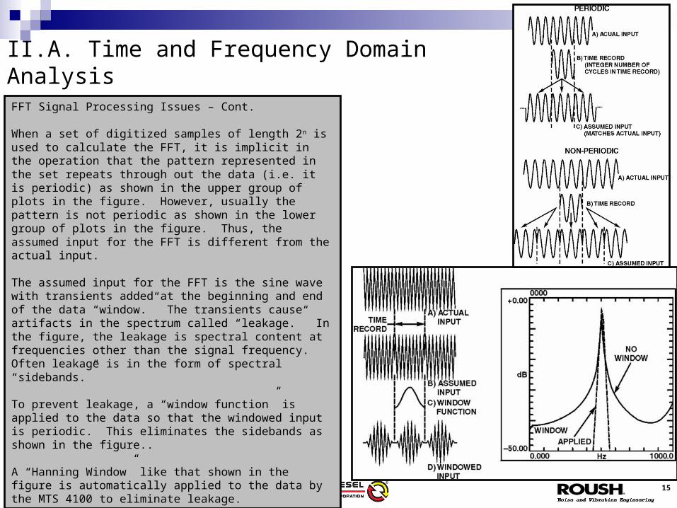
When a set of digitized samples of length 2n is used to calculate the FFT, it is implicit in the operation that the pattern represented in the set repeats through out the data (i.e. it is periodic) as shown in the upper group of plots in the figure. However, usually the pattern is not periodic as shown in the lower group of plots in the figure. Thus, the assumed input for the FFT is different from the actual input.
The assumed input for the FFT is the sine wave with transients added at the beginning and end of the data “window.” The transients cause artifacts in the spectrum called “leakage.” In the figure, the leakage is spectral content at frequencies other than the signal frequency. Often leakage is in the form of spectral “sidebands.”
To prevent leakage, a “window function” is applied to the data so that the windowed input is periodic. This eliminates the sidebands as shown in the figure..
A “Hanning Window” like that shown in the figure is automatically applied to the data by the MTS 4100 to eliminate leakage.

16
II.A. Time and Frequency Domain AnalysisFFT Signal Processing Issues – Cont.
When the signal is digitized, the value at a sample time is assigned the closest available digital value as shown in the figure. This digital “rounding off” is called quantization error.
The most obvious effect of quantization error is the limitation of the “resolution” or “dynamic range” of the instrument. The “dynamic range” is the difference between the strongest measurable signal (without overload) and the weakest measurable signal. As shown, for a 4-bit A/D values are available from 0 to 15. The “dynamic range” or “resolution” of a 4-bit A/D is 20Log10(15) = 24 dB. Similarly, the dynamic ranges of 8-bit, 12-bit, 16-bit, and 24-bit A/Ds are 48 dB, 72 dB, 96dB, and, 144 dB, respectively.
To maximize its dynamic range, the MTS 4100 is set for input signals typical of vehicle acceleration and microphone measurements; however, the MTS 4100 does not allow the inputs to be automatically ranged for getter dynamic range.


18
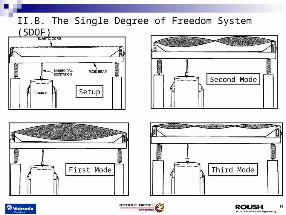
II.B. The Single Degree of Freedom System (SDOF)
Demo Description – An elastic cord is driven by a sine wave signal at its first four natural frequencies. A strobe is used to show the mode shapes.
This demonstration shows that the motion of an elastic structure is made up of specific shapes (called mode shapes or eigenshapes) associated with specific frequencies (called natural frequencies or eigenvalues).
The demonstration also shows that a strobe can be used to determine the natural frequency and mode shapes of structures undergoing relatively large displacements.
This same behavior could be shown on a truck frame, steering wheel, or seat while the truck is under operation.
Setup
19
II.B. The Single Degree of Freedom System (SDOF)
Setup
First Mode
Second Mode
Third Mode

20
II.B. The Single Degree of Freedom System (SDOF) Many of the characteristics of a vibrating system
can be examined using the SDOF System consisting of a mass, spring, and damper. The model is also known as the mass/spring/damper model.
The SDOF System model can be used to understand the behavior of engine mounts, cab mounts, steering columns, frames, and other important dynamic systems of a truck.
Even though all dynamic systems of trucks have multiple degrees of freedom, the performance of each mode is represented by the SDOF.

21
II.B. The Single Degree of Freedom System (SDOF)Why study the SDOF? – True SDOF systems are rare. For example, a truck engine on flexible engine mounts will have six different rigid-body natural frequencies.
As we saw in the previous demonstration with the elastic cord, the behavior of multiple DOF systems and continuous systems is the sum of an infinite number of modes.
The mathematical process of describing the response of a complex dynamic system as the sum of modes is called modal superposition. Modal superposition shows that the behavior of the structure for each natural frequency and mode shape is described by the behavior of the SDOF system.
Associated with each mode is a modal mass, modal stiffness, and modal damping; but these properties will be different from the global mass, stiffness, and damping.

22
II.B. The Single Degree of Freedom System (SDOF)
The frequency domain transfer function (output displacement normalized by input force as a function of frequency) is:
kcjmF
X
2
1
X() and F() are the complex amplitudes of the response displacement and the input force, respectively. The variable “” is the frequency in radians/second, and “j” is the square root of minus one.
A Note Regarding Equations – Equations are used throughout this presentation to show that the conclusions stated are strongly supported by well established theory and that the conclusions are not opinions. An understanding of the equations is not required to develop a strong understanding of vibratory systems, but some participants may feel more comfortable with the material after examining the equations.
23
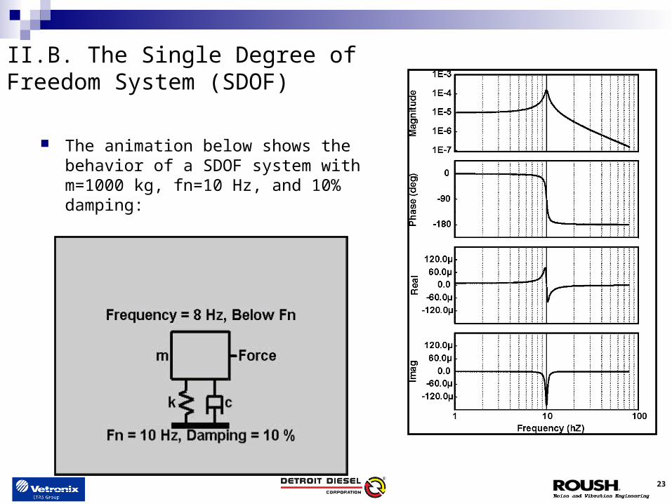
II.B. The Single Degree of Freedom System (SDOF)
The animation below shows the behavior of a SDOF system with m=1000 kg, fn=10 Hz, and 10% damping:

24
II.B. The Single Degree of Freedom System (SDOF) At low frequency (stiffness controlled region):
Near the natural frequency (damping controlled region):
At high frequency (mass controlled region):
cjmkF
mkX
1
kF
X 1
0
0
mF
X2
1

25
II.B. The Single Degree of Freedom System (SDOF)
At low frequency, the response of a forced resonant system is a function of stiffness.
Near the natural frequency, the response is very strong and is a function of damping.
At high frequency, the response weakens and is a function of mass. For example, this would be the desirable operating condition of truck engine mounts, etc. The natural frequency would be below the engine firing frequency.

26
II.B. The Single Degree of Freedom System (SDOF) Demo Description – To simulate an engine on mounts an electric motor is
suspended from elastic cords. A tap test and the MTS 4100 was previously used to determine the natural frequencies. The motor is operated discrete speeds and the peak-hold spectrum is observed using the MTS 4100.
As the motor speed passes through the natural frequencies of the dynamic system, the response increases significantly as seen on the plot.
This behavior is similar to what would be seen in an operating engine except that the engine excites more frequencies than the rotational speed. These additional engine “orders” are discussed later in the presentation.
Electric Motor with Imbalance
Base
Springs
Demonstration Setup

27
II.B. The Single Degree of Freedom System (SDOF) Demo screen shot from
MTS 4100. Resonances at low speed
(frequency). Response due to
centifugal force at high speed proportional to speed squared.

28
II.B. The Single Degree of Freedom System (SDOF)
SDOF Systems can represent torsional resonances also. Mass (kg), stiffness (N/m), and damping (N*s/m) are analogous to moment
of inertia (kg*m2), rotational stiffness (N*m), and rotational damping (N*m*s).
m
k cc
k
I
Linear System Torsional System

29
II.B. The Single Degree of Freedom System (SDOF)
The animation shows the resonance of a shaft system in a hybrid powerplant as it passes through a torsional resonance.


31
II.C. Transmissibility and Isolation
Many of the characteristics of an isolated mass (e.g. an engine on rubber mounts) can be examined using a slight variant of the previous SDOF System:

32
II.C. Transmissibility and Isolation
The transmissibility (mass response normalized by base motion as a function of frequency) is:
kcjm
kcj
Y
X
2
Lower transmissibility is better. Isolation is the reciprocal of
transmissibility. Higher isolation is better.
An understanding of the equations is not required to develop a strong understanding of vibratory systems.
33
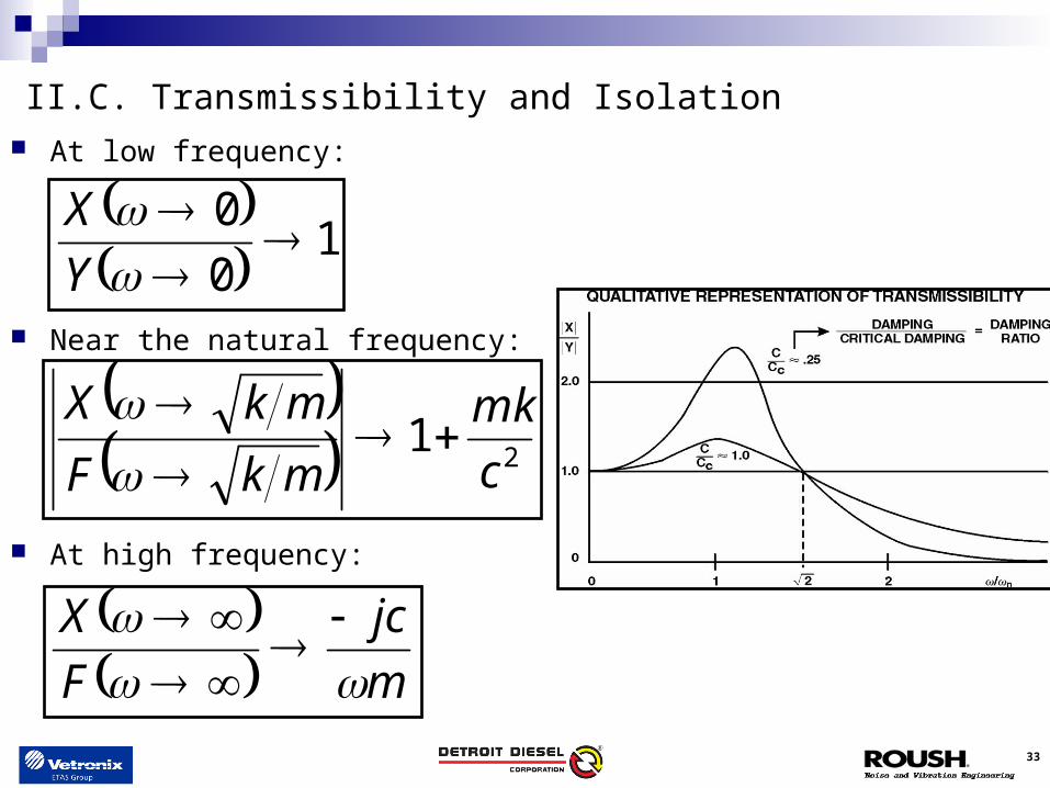
II.C. Transmissibility and Isolation At low frequency:
Near the natural frequency:
At high frequency:
2
1c
mk
mkF
mkX
1
0
0
Y
X
m
jc
F
X

34
II.C. Transmissibility and Isolation
At low frequency, the mass moves in phase with the base, and there is no isolation.
Near the natural frequency, the transmissibility is greater than one (gain rather than isolation). The gain is controlled by the ratio of the damping squared to the product of the mass and the stiffness (the damping ratio squared).
At high frequency, the transmissibility is less than one, and the gain is controlled by the ratio of damping to mass.
Overall, the goal of an effective isolation system is to have the natural frequency lower than the excitation frequency. Damping is good to have near the natural frequency, but decreases isolation at higher frequencies.

35
II.C. Transmissibility and Isolation
When motion of the engine mounts causes motion at the frame-side attachments, vibration energy is transmitted into the truck chassis.
To minimize this effect for automobiles, the static stiffness of the frame-side attachments is made relatively large (10 times).
For heavy trucks, this is not possible because the mounts are much stiffer and the frame is not relatively stiff (maybe 2 times).
A secondary isolation system (cab mounts) is necessary to keep vibration at a reasonable level.
Field experience will establish what are good values for engine and cab mount transmissibility.


37
Engine Wind Tire/Road Exhaust Intake Driveline Axle Traffic HVAC
Airborne Paths Structure-Borne Paths
SPL at Front/Rear Seat Ear Positions Vibration at Floor, Pedals, Steering
Wheel, and Seat
II.D. The Source/Path/Receiver Model
Sources
Paths
Receiver

38
II.D. The Source/Path/Receiver Model All truck vibration issues will be due to engine,
driveline, or tire orders.
This indicates that the engine (etc.) is the source of the vibration, but not necessarily the root cause because the path may be inadequate.
Inadequate paths include bad engine mounts, cab mounts, and exhaust mounts.
Inadequate paths can also include strong (or multiple) resonances of the truck structure.
Sources
Paths
Receiver

39
II.D. The Source/Path/Receiver ModelA Case Study – Several years ago Roush worked on a medium duty truck that had unacceptable vibration at a particular frequency. It was found that the truck had four major subsystems with that same natural frequency including: (1) the back panel of the cab, (2) the second acoustical mode of the cab, (3) the exhaust system, and (4) the clutch system. Presumably, the same natural frequency had been used as a minimum design target for the subsystems. The natural frequency of these subsystems was excited by the first strong torsional “order” of the engine.
In this case, the unacceptable vibration was excited by the engine, but the engine was not the root cause of the vibration issue. There was nothing wrong with the design of the cab, the exhaust system, or the clutch system. The issue was the NVH design integration. This is an example of the path being the root cause of the issue without any specific part in the path being the cause.
When designing vehicles, many-but-not-all vehicle developers check the modal alignment of the vehicle. A chart is made of all the natural frequencies of all the major subsystems of the vehicle. When natural frequencies align, the design is checked and usually changed.
Sources
Paths
Receiver

40
II.D. The Source/Path/Receiver Model For trucks without N&V issues, low frequency
noise is dominated by structural paths and high frequency noise is dominated by airborne paths.


42
II.E. Summary
The magnitude of sound or vibration vs frequency is called the spectrum and it is calculated using the FFT (Fast Fourier Transform).
For a resonant SDOF (Single Degree of Freedom) system:• Low frequency is stiffness controlled.• Near the natural frequency is damping controlled.• High frequency is mass controlled.

43
II.E. Summary
Transmissibility is the reciprocal of isolation. Lower transmissibility is better. For the modified SDOF model transmissibility:
• Low frequency, transmissibility is approximately one.• Near the natural frequency, transmissibility is higher than one
and controlled by the damping ratio squared (c2/km).• High frequency, transmissibility is less than one and controlled
by damping and mass (c/m). Frame flexibility reduces the effectiveness of engine mounts.

44
II.E. Summary
The source/path/receiver model shows that the root cause of a N&V issue may be the path rather than the source.
Paths may be mounts or structural resonances. Low frequency noise is normally dominated by structural paths,
and high frequency noise is normally dominated by airborne paths.
45
II.F. Discussion
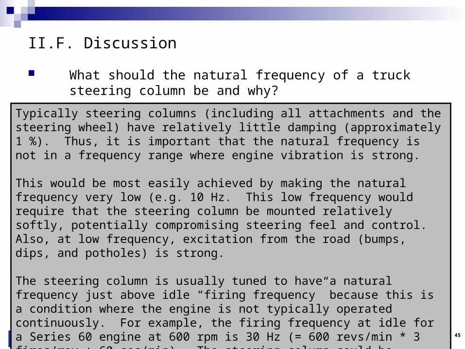
What should the natural frequency of a truck steering column be and why?
Typically steering columns (including all attachments and the steering wheel) have relatively little damping (approximately 1 %). Thus, it is important that the natural frequency is not in a frequency range where engine vibration is strong.
This would be most easily achieved by making the natural frequency very low (e.g. 10 Hz. This low frequency would require that the steering column be mounted relatively softly, potentially compromising steering feel and control. Also, at low frequency, excitation from the road (bumps, dips, and potholes) is strong.
The steering column is usually tuned to have a natural frequency just above idle “firing frequency” because this is a condition where the engine is not typically operated continuously. For example, the firing frequency at idle for a Series 60 engine at 600 rpm is 30 Hz (= 600 revs/min * 3 fires/rev ÷ 60 sec/min). The steering column could be designed to have a natural frequency of 36 Hz which would correspond to the firing frequency at 720 rpm.

46
II.F. Discussion
Steering wheel vibration in a truck is excessive at the engine firing order. Name two reasons why excessive engine vibration may not be the root cause. Hint – source/path/receiver model.
The response of the steering wheel is the product of the input forcing function (vibration from the engine source) and the vibration transfer function. If the engine vibration (source) is within normal limits, the transfer function (path) of the steering wheel is too large at the engine firing frequency.
(1) The natural frequency of the steering column might be lower (and closer to a “significant engine-vibration-order”) than intended due to loose fasteners or a poor fit at the attachment points.
(2) The steering wheel is mounted to the cab, so deficient cab mounts would contribute to excessive steering wheel vibration. In this case, vibration levels would also be higher than normal in other parts of the cab. Likewise, deficient engine mounts would contribute to excessive steering wheel vibration with higher than normal vibration levels in other parts of the truck.

47
II.F. Discussion
An off-road truck manufacturer increased the stiffness of the engine mounts to increase durability. Vibration at idle is significantly worse. Name two reasons why. Hint – transmissibility.
Normally engine mounts are designed so that the rigid-body natural frequencies of the engine/mount system are lower than the engine firing frequency at idle. This is a fairly low frequency (less than 30 Hz at 600 rpm idle). Thus, the excursion of the mounts under the influence of road inputs can be significant. This negatively impacts the durability of the mounts and can also lead to perceivable “after-shake” of the engine. (1) Vibration at idle is worse because the engine mounts were made stiffer, and this moved the rigid-body natural frequencies closer to the idle frequency. Also, the stiffer mounts would make the ratio of mount stiffness to frame stiffness worse.
Engine mounts can be tuned to “decouple” the modes of the engine. This means that the “roll mode” of the engine is not associated with engine bounce, pitch, etc. Likewise, the pitch mode is not associated with engine roll, bounce, and pitch; and so on. (2) Vibration at idle is worse because changing the mount rates increased the coupling of rigid-body modes of the engine/mount system.


49
III. Vibration
A. Sensitivity to vibration
B. Forced versus resonant vibration
C. Rotating machinery vibration, orders, and critical speed
D. Vehicle driveline issues
E. Summary
F. Discussion
50
III.A. Sensitivity to Vibration
Human sensitivity to vibration depends on a large number of factors including the part of the body, body position, the nature of the vibration (shock or continuous), and direction of vibration.
A sampling of vibration sensitivity data is presented.

51
III.A. Sensitivity to Vibration The perception of vibration is approximately linear (i.e. twice as much
acceleration is perceived as twice as much acceleration). The figure (Cyril M. Harris and Charles E. Crede, Shock and Vibration
Handbook, Second Ed., McGraw-Hill, 1976) shows the limit of perception, unpleasantness, and intolerability as a function of frequency.
The difference between barely perceivable and intolerable is approximately 100X. (3,000,000X for human hearing).
Sensitivity to vibration declines steeply above 200 Hz.
Note that 1 g = 9.8 m/s2.
Vibration Perception
0.001
0.01
0.1
1
1 10 100
Frequency (Hz)
Acc
ele
rati
on
(g
, pe
ak)
Threshold ofPerception
Intolerable
Unpleasant

52
III.A. Sensitivity to Vibration ISO 5349-1 provides exposure limits
for hand vibration.
The standards are for the vector addition of all directions.
The accelerations are multiplied by the weighting factor shown in the figure, so the highest susceptibility is around 12 Hz.
The 8-hour levels are 26 m/s2, 14 m/s2, 7 m/s2, and 3.7 m/s2 for 1, 2, 4, and 8 years of exposure. These levels may be expected to produce episodes of finger blanching in 10% of operators exposed.
Symptoms are rare for operators with an 8-hour level of less than 2 m/s2 and unreported for 1 m/s2.
Weighting Factor for Hand Vibration Data
0.01
0.10
1.00
1 10 100 1000
Frequency (Hz)W
eig
hti
ng
Fac
tor

53
III.A. Sensitivity to Vibration Whole body vibration can cause operator fatigue. The figure (Jens Trampe Broch, Mechanical Vibration and Shock
Measurement, Bruel and Kjaer, 1980) shows vibration exposure versus exposure time.
The highest susceptibility is between 4 Hz and 8 Hz.Vibration Exposure Criteria for Fatigue, Vertical, Seated,
Whole-Body
0.1
1
10
1.00
1.25
1.60
2.00
2.50
3.15
4.00
5.00
6.30
8.00
10.0
0
12.5
0
16.0
0
20.0
0
25.0
0
31.5
0
40.0
0
50.0
0
63.0
0
80.0
0Third-Octave-Band Frequency
Acc
eler
atio
n (
m/s
^2,
rm
s)
24 hour16 hour8 hour4 hour2.5 hour1 hour25 min16 min1 min
54
III.A. Sensitivity to Vibration
Some companies use DVD (vibration dose value) to access ride harshness.
From Ken Horste, Ford Motor Company, SAE Paper 95373, 1995.
Primarily used for shift quality and driving over impact strips.
To calculate DVD, the acceleration data is bandpass filtered between 1 Hz and 31.9 Hz. Then the filtered acceleration is taken to the fourth power and integrated numerically.


56
III.B. Forced vs Resonant Vibration
Vibration in structures can be induced without resonance. For example, low-frequency rigid body motion, and motion of non-resonant structures (analogous to a pile of sand).
The figure shows both forced and resonant vibration behavior. (Accelerometer mounted on Series 60 engine).
0 1000100 200 300 400 500 600 700 800 90050 150 250 350 450 550 650 750 850 950
HzFront Mount Y:+Y (CH25)
1020
2020
1100
1200
1300
1400
1500
1600
1700
1800
1900
1150
1250
1350
1450
1550
1650
1750
1850
1950
rpm
Tac
ho1
(T1)
100e-3
50
1
10
200e-3
300e-3
400e-3
500e-3600e-3
800e-3
2
3
4
56
8
20
30
Log
( m/s
2 )
3.00
494.6
Forced Vibration
Strong ResonantVibration

57
III.B. Forced vs Resonant Vibration
It is important to distinguish forced and resonant vibration because the method of treatment is fundamentally different.
Resonant vibration is treated by adding damping or changing the resonant frequency.
Forced vibration is treated with isolation or reducing the forcing amplitude (e.g. improved balancing).
0 1000100 200 300 400 500 600 700 800 90050 150 250 350 450 550 650 750 850 950
HzFront Mount Y:+Y (CH25)
1020
2020
1100
1200
1300
1400
1500
1600
1700
1800
1900
1150
1250
1350
1450
1550
1650
1750
1850
1950
rpm
Tac
ho1
(T1)
100e-3
50
1
10
200e-3
300e-3
400e-3
500e-3600e-3
800e-3
2
3
4
56
8
20
30
Log
( m/s
2 )
3.00
494.6


59
III.C. Rotating Machinery Vibration, Orders, and Critical Speed
Rotating equipment includes truck engine, driveline, and tires.
If an event happens once per revolution it is called “first order.”
Imbalance is an example of a first order vibration source.
If an event happens twice per revolution it is “second order.”
Vibration due to driveline “Cardan Joints” (U-Joints) is an example of a second order vibration source.
Orders can be non-integer. For example, due to FEAD pulleys, transmissions, differentials, etc.

60
III.C. Rotating Machinery Vibration, Orders, and Critical Speed The truck engine produces vibration and noise at many orders. Orders appear as straight, diagonal lines in the “Waterfall Plot” or “Campbell
Diagram.” Resonances appear as straight vertical lines.
0 1000100 200 300 400 500 600 700 800 90050 150 250 350 450 550 650 750 850 950
HzFront Mount Y:+Y (CH25)
1020
2020
1100
1200
1300
1400
1500
1600
1700
1800
1900
1150
1250
1350
1450
1550
1650
1750
1850
1950
rpm
Tac
ho1
(T1)
100e-3
50
1
10
200e-3
300e-3
400e-3
500e-3600e-3
800e-3
2
3
4
56
8
20
30
Log
( m/s
2 )
3.00
494.6
3rd
Order6th
Order9th
Order

61
III.C. Rotating Machinery Vibration, Orders, and Critical SpeedWhy does the Series 60 engine have vibration at certain orders?
The Series 60 is an “even fire” six cylinder engine. Every revolution of the engine takes the crankshaft, rod, and pistons through a complete cycle. Thus, crankshaft imbalance produces first order vibration. Other multiples of first order (2nd, 3rd, etc.) are also produced by the rotation of the crankshaft due to the “non-sinusoidal” motion of the pistons and rods (Charles Fayette Taylor, The Internal Combustion Engine in Theory and Practice, Volume 2, MIT Press, 1979).
Every two revolutions the cam/injector system goes through a cycle. Thus, the cam drive produces half order vibration. Other multiples of half order (1.0, 1.5, 2.0, etc.) are also produced by motion of the cam drive due to the non-sinusoidal torque load. The 4.5 order is strong.
Every two revolutions (720 degrees) a cylinder goes through a complete combustion cycle (intake, compression, ignition, and exhaust), but this is an even fire engine, so every 120 degrees (720/6) the combustion process repeats. Thus, combustion produces 3rd order vibration and multiples (6th, 9th, 12th order, etc.).
The Series 60 engine has an air pump that produces vibration at 1.2 engine order because it is driven by a gear train at 1.2 times the speed of the crankshaft.

62
III.C. Rotating Machinery Vibration, Orders, and Critical Speed
Shafts have a first bending natural frequency. When the rotational speed of the shaft is at this natural frequency the imbalance excites this natural frequency, and the amplitude of vibration is only limited by the damping. Damping is usually very small because the shaft is like a rotating banana, so there is no alternating stress. The shaft speed at which the rotational speed matches the natural frequency is called the “critical speed.”
Shaft systems (like a heavy truck driveshaft) are almost always designed so that the shaft never operates at the critical speed.
At the critical speed, the shaft deformations become larger which produces even larger imbalance. The situation (deformation producing larger imbalance and imbalance creating larger deformation) can become unstable, and the shaft can experience catastrophic failure.

63
III.C. Rotating Machinery Vibration, Orders, and Critical Speed
Sometimes shafts must spin at speeds greater than critical speed. For example, high speed race cars and steam turbines at electrical power plants.
For the race car, the driveshaft critical speed is moved to a lower frequency, so the driveshaft quickly accelerates through the critical speed and never dwells at the critical speed.
For the steam turbine, the natural frequencies are all known in advance. When the turbine is put into service from a stop, the turbine is quickly accelerated through the critical speeds to prevent damage. The steady-state speed of the turbine is not located near a critical speed.
Note that vehicles with one-piece driveshafts are usually speed limited to prevent the vehicle from operating at the critical speed of the driveshaft. This is approximately 100 mph for pickup trucks and 130 mph for RWD sports cars.


65
III.D. Vehicle Driveline Issues
Vehicle driveline issues usually occur at the first and second order driveline frequency (i.e. once or twice per driveshaft revolution).
First order disturbances are associated with “imbalance” and “runout.”
Second order disturbances are associated with “Cardan Joints” and “Driveline Angles.”
66
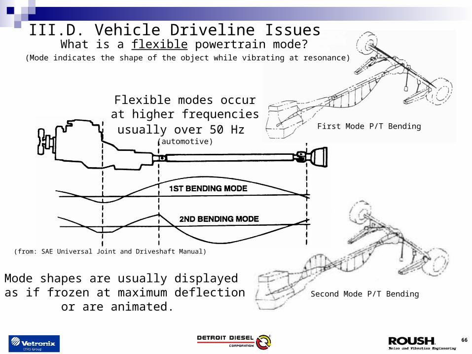
What is a flexible powertrain mode? (Mode indicates the shape of the object while vibrating at resonance)
(from: SAE Universal Joint and Driveshaft Manual)
First Mode P/T Bending
Second Mode P/T Bending
Flexible modes occurat higher frequenciesusually over 50 Hz
(automotive)
Mode shapes are usually displayed as if frozen at maximum deflection
or are animated.
III.D. Vehicle Driveline Issues

67
where:Nc= Revolutions per minute, rpmE = Modulus of elasticity, psi I = Area moment of inertia, in4
g = Acceleration due to gravity, in/s2
W = Total weight of shaft, lbL = Shaft length between supports, in
330
WL
EIgNc
General Equation:
Round TubularSteel Shaft:
2
22
000,705,4L
ddN io
c
Equations are from the SAE Universal Joint and Driveline Design Manual
Driveshaft Critical Speed Calculation(Pin-Pin)
where:do= outside diameter, indi = Inside diameter, inL = Shaft length, innote: for solid shaft, di = 0(Hollow shaft gives higher Nc)
Thinner wall =
Higher frequency
III.D. Vehicle Driveline Issues
68
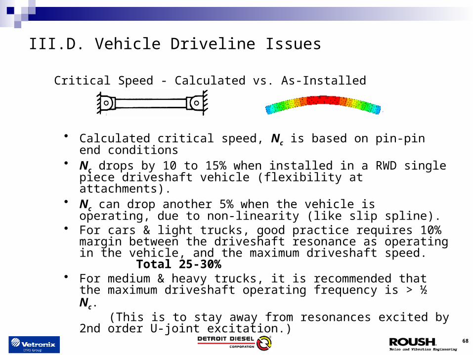
Critical Speed - Calculated vs. As-Installed
Calculated critical speed, Nc is based on pin-pin end conditions Nc drops by 10 to 15% when installed in a RWD single piece driveshaft
vehicle (flexibility at attachments). Nc can drop another 5% when the vehicle is operating, due to non-
linearity (like slip spline). For cars & light trucks, good practice requires 10% margin between the
driveshaft resonance as operating in the vehicle, and the maximum driveshaft speed. Total 25-30%
For medium & heavy trucks, it is recommended that the maximum driveshaft operating frequency is > ½ Nc.
(This is to stay away from resonances excited by 2nd order U-joint excitation.)
III.D. Vehicle Driveline Issues

69
Driveline Roughness, Drumming/Boom, & Shudder
Definitions Driveline arrangements Excitation Path Unbalance and runout Pitch line runout Transverse AWD Driveline angles
III.D. Vehicle Driveline Issues

70
Driveline Disturbance Definitions:
D/L Roughness – mid frequency vibration (50–80 hz), usually at vehicle speeds above 50 MPH (automotive), and can have boom/drumming associated with it.
III.D. Vehicle Driveline Issues
71
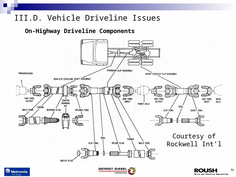
On-Highway Driveline Components
Courtesy ofRockwell Int’l
III.D. Vehicle Driveline Issues

72
Driveline Excitations
Unbalance Runout in driveline Slop in driveline Driveline angles Pinion pitch line runout (first order gear rotation error, explained
in gear section)
Path is usually structure-borne
III.D. Vehicle Driveline Issues
Note that “Unbalance” and “Imbalance” are the same.

73
Potential Contributors to 1st Order Driveline Excitation
III.D. Vehicle Driveline Issues

74
System Related Issues
III.D. Vehicle Driveline Issues
75
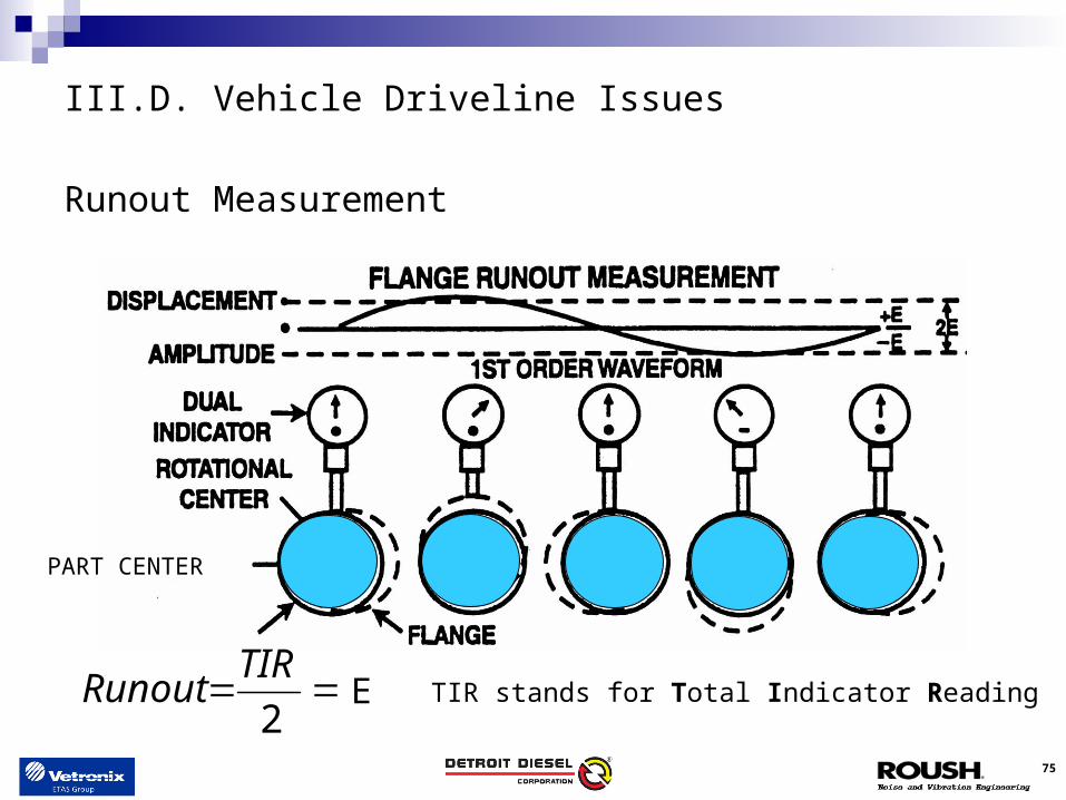
Runout Measurement
2
TIRRunout E
PART CENTER
TIR stands for Total Indicator Reading
III.D. Vehicle Driveline Issues

76
Effect of Unbalance
2Rg
WF
where:W = Weight g = gravityR = radius of mass center = angular velocity
(from: SAE Universal Joint and Driveshaft Manual)
Typicalpassengervehiclespec: <.4
10,000 RPM !!!
III.D. Vehicle Driveline Issues
Note that “Unbalance” and “Imbalance” are the same.
77
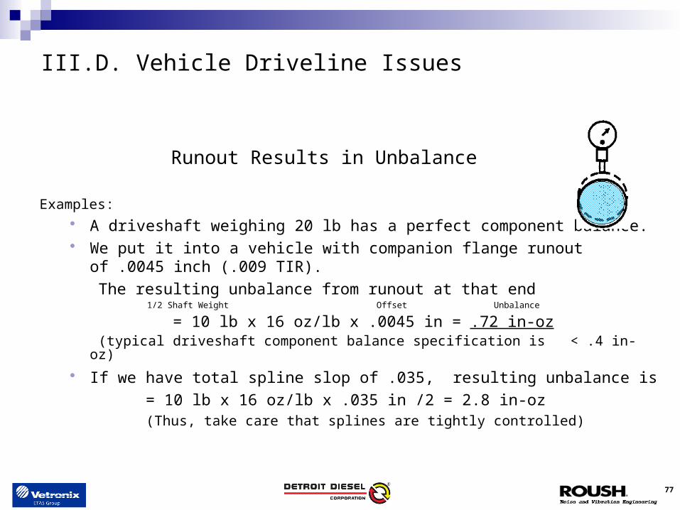
Runout Results in Unbalance
Examples: A driveshaft weighing 20 lb has a perfect component balance. We put it into a vehicle with companion flange runout of .0045 inch (.009
TIR).
The resulting unbalance from runout at that end 1/2 Shaft Weight Offset Unbalance
= 10 lb x 16 oz/lb x .0045 in = .72 in-oz (typical driveshaft component balance specification is < .4 in-oz)
If we have total spline slop of .035, resulting unbalance is
= 10 lb x 16 oz/lb x .035 in /2 = 2.8 in-oz(Thus, take care that splines are tightly controlled)
III.D. Vehicle Driveline Issues

78
Contributors to Unbalance & Runout
Spline clearance/slop
Bent shafts (Driveshaft or transmission)
Transmission unbalance contribution (have seen up to 10 in-oz in large automatic,
that’s a lot!)
System balancing – match mounting of components
Transmission vs. Axle sensitivity - the end attached to the axle (including AWD) is
usually 2 or more times as sensitive, because of mass ratio & path
III.D. Vehicle Driveline Issues

79
Tire/Wheel Inputs
Out-of-Round
Force Variation
Runout
Imbalance
Force Variation
Oval Shape
Force Variation
1st O
rder
2nd O
rder
3rd O
rder
4 W
heel
s
LF RF
RRLR
III.D. Vehicle Driveline Issues

80
Tire Frequency Calculation
ratio aspectwidth sectiondiameterwheeldiametertiremile
rev
2
850,20850,20
The following empirical formula was developed (by General Motors):
where: height sectiontirediameterwheeldiametertire 2tire section height = section width x aspect ratio
then:
6060
MPHmilerev
min
hr
hr
mi
mile
revRPM
60)(
RPMhzfrequency and:
Example for a P205/60R15 tire: 84460.
4.25205215
850,20
mmin
mminmile
rev
Notes:Tire load and pressure - have little effect on revs/mile due to the fact that the radial belts and tread have a very high hoop strength, acting like a track.Tread wear also has little effect since tire cords tend to stretch with age as tread wears. Usually <2% change with pressure, load, and/or wear.% slip - due to power transferred and road conditions ( wet, dry, sand, ice, etc) make more difference in revs/mile than any of the above.
III.D. Vehicle Driveline Issues

81
Driveline Disturbances
Hardware comparison Cardan or Hooke Universal Joints CV joints – not covered Flex couplings – not covered
Discussion Rotational errors
Cardan Joints
III.D. Vehicle Driveline Issues

82
Cardan or Hooke Universal Joint
(from: SAE Universal Joint and Driveshaft Manual)
III.D. Vehicle Driveline Issues

83
Cardan Joint Developing Non-Uniform Motion
Courtesy of Dana Corp.
III.D. Vehicle Driveline Issues

84
Measurement of Driveline Angles
This analysis assumesno offset from top view.
III.D. Vehicle Driveline Issues

85
Driveline Angle Change
III.D. Vehicle Driveline Issues

86
Driveline Angle Change
(from: SAE Universal Joint and Driveshaft Manual)
22
rearfrontresidual
Proper phasing of the joints results in some cancellation of the torsional transmission errors.
or residual angles
III.D. Vehicle Driveline Issues

87
Residual Angle at Front/Rear Angle Differences of 0.5, 1.0, and 2.0 Degrees
0.00
1.00
2.00
3.00
4.00
5.00
6.00
7.00
2 3 4 5 6 7 8 9 10 11 12 13
Front/Rear Average Working Angle - Deg.
2.0 DegreeDifferenceFront to Rear
1.0 DegreeDifferenceFront to Rear
0.5 DegreeDifferenceFront to Rear
Probable LimitFor AcceptanceDrive-Line
R O
U S
H A
N A
T R
O L
Gen
erat
ed R
esid
ual
Ang
le -
Deg
.
Mark Jackson
Roush Industries
February 1998
22
rearfrontresidual
III.D. Vehicle Driveline Issues

88
Rotational Inertia Effects
1= 2 & 3 - The equal angles cancel speed errors, but the driveshaft inertia is being accelerated and decelerated twice per revolution. This results in cyclic torque disturbances within the driveline system. Forces generated can be significant, especially for large angles & heavy shafts.
III.D. Vehicle Driveline Issues

89
Two Piece Driveline & Center Bearing
Couples generated at the joints result in take-off shudder The rotating secondary couples, Cn are a function of the driveline torque and the
angles at the Cardan joints:
where: T = driveline torque
n = joint angle
The forces generated are dependant on shaft lengths fn usually 12-18 hz, 12-18 mph
Low speed - you go through fn quickly under high torque
Low torque moment when steady state at fn
Cn = T tann
Center SupportBearingC1 C2
C3
Lateral
Vertical
SAE Universal Joint and Driveshaft Manual
III.D. Vehicle Driveline Issues

90
2 Piece Driveline & Center Bearing
65 hz
18 hz
CenterAngle
tan
0o .0002o .0354o .0706o .1058o .14010o .17615o .268
(from: SAE Universal Joint and
Driveshaft Manual)
Keep the angles small!
Couples
Cn = T tann
C1
C3
C2
23
Typical shaft support bearing transmissibility characteristics
due to unbalance
1
III.D. Vehicle Driveline Issues


92
III.E. Summary
The perception of vibration is approximately linear (i.e. twice as much acceleration is perceived as twice as much acceleration).
The difference between barely perceivable and intolerable vibration is approximately 100X.
Sensitivity to vibration declines steeply above 200 Hz.
ISO 5349-1 provides exposure limits for hand vibration. Limits are specified for various vibration levels and exposure times. Symptoms are rare for operators with an 8-hour level of less than 2 m/s2 and unreported for 1 m/s2.

93
III.E. Summary
Vibration can be either forced or resonant. Resonant vibrations are lines at specific frequencies on the Campbell Diagram.
Forced vibrations are treated by reducing the forcing levels and adding isolation.
Resonant vibrations are treated by adding damping or moving the resonant frequency.
If an event happens once per revolution (like rotating imbalance), it produces first order vibration.
If an event happens twice per revolution (like a Cardan Joint), it produced second order vibration, etc.
Orders appear as angled lines in the Campbell Diagram.

94
III.E. Summary
The Series 60 engine produces vibration at many orders including: 1st order (engine imbalance); 1.2 order (air pump); 4.5 order and various half orders (cam/injector drive); and 3, 6, 9, … order (engine combustion).
The speed at which a shaft (like a driveshaft) is rotating at its first bending natural frequency is called the critical speed.
Catastrophic failure can occur at the shaft critical speed.
Driveline imbalance and runout produce first order driveline vibration.
Driveline angles must be properly matched to minimize second order vibration due to the Cardan joints. Suspension movements usually cause driveline angles to change.
Tires produce vibration because of imbalance, runout, out-of-round, and force variation.
95
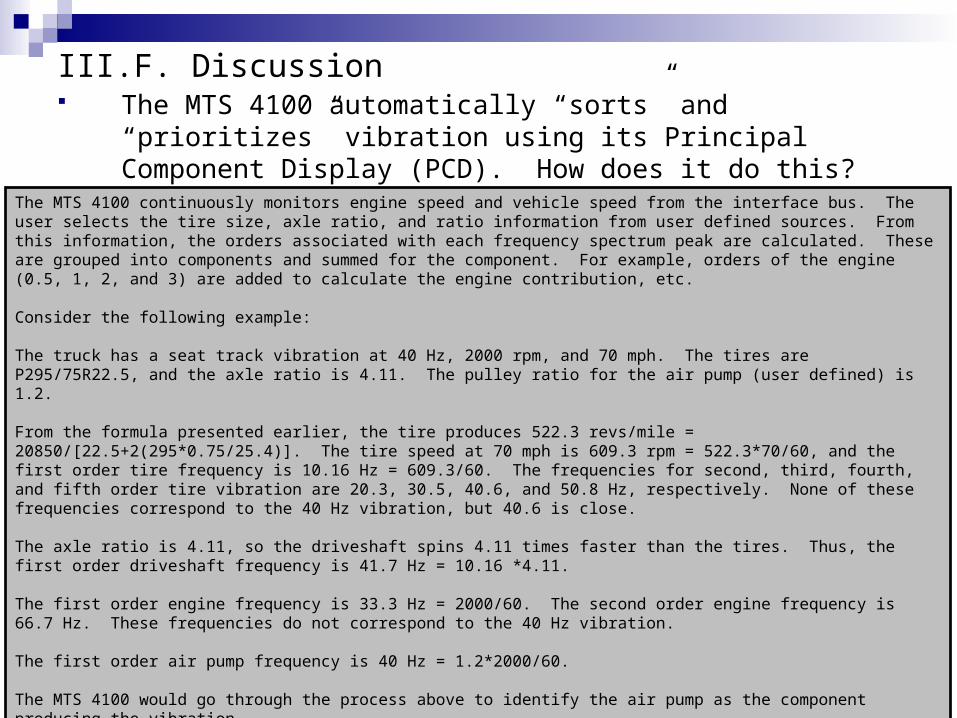
III.F. Discussion The MTS 4100 automatically “sorts” and “prioritizes” vibration
using its Principal Component Display (PCD). How does it do this?
The MTS 4100 continuously monitors engine speed and vehicle speed from the interface bus. The user selects the tire size, axle ratio, and ratio information from user defined sources. From this information, the orders associated with each frequency spectrum peak are calculated. These are grouped into components and summed for the component. For example, orders of the engine (0.5, 1, 2, and 3) are added to calculate the engine contribution, etc.
Consider the following example:
The truck has a seat track vibration at 40 Hz, 2000 rpm, and 70 mph. The tires are P295/75R22.5, and the axle ratio is 4.11. The pulley ratio for the air pump (user defined) is 1.2.
From the formula presented earlier, the tire produces 522.3 revs/mile = 20850/[22.5+2(295*0.75/25.4)]. The tire speed at 70 mph is 609.3 rpm = 522.3*70/60, and the first order tire frequency is 10.16 Hz = 609.3/60. The frequencies for second, third, fourth, and fifth order tire vibration are 20.3, 30.5, 40.6, and 50.8 Hz, respectively. None of these frequencies correspond to the 40 Hz vibration, but 40.6 is close.
The axle ratio is 4.11, so the driveshaft spins 4.11 times faster than the tires. Thus, the first order driveshaft frequency is 41.7 Hz = 10.16 *4.11.
The first order engine frequency is 33.3 Hz = 2000/60. The second order engine frequency is 66.7 Hz. These frequencies do not correspond to the 40 Hz vibration.
The first order air pump frequency is 40 Hz = 1.2*2000/60.
The MTS 4100 would go through the process above to identify the air pump as the component producing the vibration.

96
III.F. Discussion
Is the vibration only observed at one vehicle speed or one engine speed (resonant vibration), or is it spread over a wide speed range (forced vibration)?
If there is a bad engine mount, there might be one engine speed at which the vibration is worst, but higher levels of vibration will be obvious at other engine speeds as well. This would be an example of a forced vibration issue.
Similarly, if the driveline angles are not right, there will be vehicle speeds at which the vibration is worst, but higher levels of vibration will be observed at other vehicle speeds.

97
III.F. Discussion
If the same vibration is observed in different gears, does it follow speed (tire/driveline) or engine speed (engine)?
Engine vibration issues track with engine speed even in different gears. Tire and driveline issues track with vehicle speed. Note that engine loads changes in different gears, and there may be a combination of engine and tire/driveline issues, so data from the MTS 4100 (rather than seat-of-pants) may be necessary.

98
III.F. Discussion
Is the vibration engine-torque sensitive?
Vibration issues can sometimes be identified by their sensitivity to engine torque. For example, axle whine is very sensitive to torque, driveline issues are moderately sensitive to torque, and tire issues are relatively insensitive to torque.
99
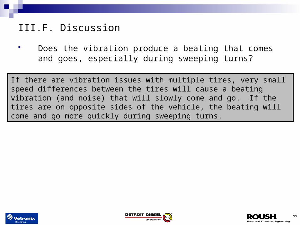
III.F. Discussion
Does the vibration produce a beating that comes and goes, especially during sweeping turns?
If there are vibration issues with multiple tires, very small speed differences between the tires will cause a beating vibration (and noise) that will slowly come and go. If the tires are on opposite sides of the vehicle, the beating will come and go more quickly during sweeping turns.


101
IV. Sound and Sound Quality
A. Decibels and A-weighting
B. Beating, fluctuation, roughness, loudness, sharpness, and knock
C. Passby noise procedure and stationary noise requirement

102
IV.A. Decibels and A-Weighting Human hearing is non-linear and is a function of both frequency
and loudness. The variation of frequency/loudness dependence of perceived
loudness (acute hearing) is shown in the figure (Robinson and Dodson, British Journal of Applied Physics, 7, 166(1956) and ISO R226-1961).
Equal Loudness Curves

103
IV.A. Decibels and A-Weighting
A, B, and C Weighting Filters
-70
-60
-50
-40
-30
-20
-10
0
10
16
25
40
63
10
0
16
0
25
0
40
0
63
0
10
00
16
00
25
00
40
00
63
00
10
00
0
16
00
0
Third-Octave-Band Frequency (Hz)
Gai
n (
dB
)
A-Weighting
B-Weighting
C-Weighting
To construct instruments that would measure perceived sound levels, A-, B-, and C-Weighting filters were developed.
The filters are applied so that measured values are approximately equal to perceived values according to the equal loudness curves.
Originally, the A-Weighting was used for levels below 55 dB, B-Weighting was used for 55-85 dB, and C-Weighting was used above 85 dB. For various reasons, A-Weighting (dBA) is the primary metric used today.
Equal Loudness Curves

104
IV.B. Decibels and A-Weighting
Decibel Facts
• The decibel is named for Alexander Graham Bell.
• Perceived doubling of loudness is 10 dB, while actual doubling of sound pressure level is 6 dB. Note: “deci” + “bel”
• Smallest perceivable change in sound is 1 dB.
• Quietest perceived sound is 0 dBA.
• Threshold of pain is approximately 130 dBA.
• Dynamic range of human ear (0 to 130 dBA) is 3,000,000 times.
)620/(20)( PaePLogdBL rms


106
IV.B. Beating, Fluctuation, Roughness, Loudness, Sharpness, and Knock With digital computers, the perceived loudness can be calculated by
applying the equal loudness curve correction directly to recorded data (rather than using the A-, B-, or C-Weighting curves).
Loudness can be expressed in dB Phones or in Sones. Sones are arranged so that sound which is perceived as twice as loud
has twice the Sones value. Heavy truck interior levels at highway speed are probably approximately 10 Sones while underhood levels are approximately 100 Sones (sounds ten times louder).
Note 40 dBA is approximately equal to 1 Sone.

107
IV.B. Beating, Fluctuation, Roughness, Loudness, Sharpness, and Knock “Beating” or
“Modulation” describes a signal with amplitude modulation of 1 Hz to 10 Hz. Worst at 4 Hz.
“Roughness” describes a signal with amplitude modulation of 10 Hz to 200 Hz. Worst at 70 Hz.
500 Hz
500 Hzwith 4 HzModulation
500 Hzwith 70 HzRoughness
500 Hz, 70 Hz Roughness
-1.0
-0.5
0.0
0.5
1.0
0.0 0.1 0.2 0.3 0.4 0.5
Time (s)
Sig
nal
(vo
lts)
500 Hz, 70 Hz Roughness
-1.0
-0.5
0.0
0.5
1.0
0.0 0.1 0.2 0.3 0.4 0.5
Time (s)S
ign
al (
volt
s)
500 Hz, 70 Hz Roughness
-1.0
-0.5
0.0
0.5
1.0
0.0 0.1 0.2 0.3 0.4 0.5
Time (s)
Sig
nal
(vo
lts)
108
IV.B. Beating, Fluctuation, Roughness, Loudness, Sharpness, and Knock “Sharpness” describes how sharp a signal sounds. It is a
combination of spectral shape and loudness.
Sharp NoiseProduced ByExhaust Flex
Coupling
NoiseWith Sharpness
Reduced

109
IV.B. Beating, Fluctuation, Roughness, Loudness, Sharpness, and Knock
“Knock” describes the degree of knock. Usually a metric is selected based on the particular nature of the noise.
The ratio of the peak transient loudness to the average loudness can be used. Kurtosis can sometimes be used.
The character of the knock can vary by application. Knock and terms like it are called “Semantic Differentials.”
Series 60At Idle
Electric AirPump with
Light Knock
Electric AirPump with
Strong Knock


111
IV.C. Passby Testing
The EPA standard for external heavy truck noise is the Code of Federal Regulations 40CFR205 which requires noise passby levels of 80 dBA or less when tested per SAE J366.
The standard involves full throttle acceleration of the heavy truck tractor through rated engine speed while peak sound levels are measured at 50 ft.
The noise levels are 6 dBA louder than those allowed for cars in the US and 12 dBA louder than those allowed for cars in Europe.
Engine - Front of Engine44%
Engine - Oil Pan36%
Engine -Other NoiseSources
20%
Passby Noise Sources for a Class 8 Truck Powered by a Series 60 Engine

112
IV.C. Passby Testing
Truck is accelerated from the acceleration line to the end line. Gears selected so that approach engine speed is no more than 67% of maximum rated speed (MRS) and MRS is achieved in the indicated zone.
Microphones
AccelerationLine
EndLine
50 ft60 ft
100 ft Reach Max Speed in Zone
Truck

113
IV.C. Stationary Testing
DDC N&V engineers use stationary testing for auditing and competitive benchmarking purposes. Stationary noise is not an EPA requirement.
Testing is performed per the SAE J1096 standard. The engine is accelerated (WOT) from idle to governed speed,
held steady to stabilize, and then decelerated to idle with no throttle.
Testing is performed in a large paved area free from obstructions for 100 ft.
Microphones are placed 50 ft from the centerline of the truck even with the rear of the cab.
The maximum A-weighted sound level is recorded. Additional microphones are sometimes used at the front and rear
of the truck to help identify noise sources.


115
V. N&V Features of DDC Engines – Current and 2007
A. Engine Mounting System
B. Isolated Oil Pan
C. Isolated Rocker Cover
D. Crankshaft Damper
E. Lined Bellows Exhaust Manifold

116
V.A. Pre-2007 Engine Mounts
Rear engine mounts

117
V.A. 2007 Engine Mounts
Front engine mount
Rear engine mount

118
V.B. Isolated Oil Pan
-composite oil pan with isolating/sealing gasket
-isolating gasket
-oil pan sleeve/bolt assembly with grommet

119
V.C. Isolated Rocker Cover
-composite rocker cover with isolating/sealing gasket
-isolating gasket
-rocker cover sleeve/bolt assembly with grommet

120
V.D. Crankshaft Damper
-function of the crankshaft viscous damper is to minimize torsionalvibration present in broad operating frequency ranges

121
V.E. Lined Bellows Exhaust Manifold
-current S60 exhaust manifold configuration with fey ring design
-2007 S60 exhaust manifold configuration with lined Bellows design
NVH ISSUE
Without internal Bellows liner, “chirp” noise present
during engine operation

122
V.E. Lined Bellows Exhaust Manifold Series 60 ‘Chirp’ Noise – Sound Quality Comparison
700 800 900 1000 1100 1200 1300 1400 1500 1600 1700 1800 1900 2000 2100
RPM
65
70
75
dB
Truck 904 Original Configuration Neutral Run Up 2_pp Interior Mic_DRE S Truck 904 With Lined Bellows Neutral Run Up_pp Interior Mic_DRE S
Measurement: APS Graphic: Sum level Amplitude Type: rm s Statistical Parameter:
700 800 900 1000 1100 1200 1300 1400 1500 1600 1700 1800 1900 2000 2100
RPM
20
25
30
35
40
sone
Truck 904 Original Configuration Neutral Run Up 2_pp Interior Mic_DRE S Truck 904 With Lined Bellows Neutral Run Up_pp Interior Mic_DRE S
Measurement: Instat. loudness Graphic: Instationary loudness Amplitude Type: lin Statistical Parameter:
700 800 900 1000 1100 1200 1300 1400 1500 1600 1700 1800 1900 2000 2100
RPM
1.10
1.15
1.20
1.25
1.30
1.35
acum
Truck 904 Original Configuration Neutral Run Up 2_pp Interior Mic_DRE S Truck 904 With Lined Bellows Neutral Run Up_pp Interior Mic_DRE S
Measurement: Sharpness Graphic: Sharpness Amplitude Type: lin Statistical Parameter:
SOUND PRESSURE LEVEL HIGHER ON ENGINEWITH BELLOWS LINERS
OVERALL LOUDNESS IS ALMOSTEQUAL WITH OR WITHOUT LINERS
SHARPNESS CLEARLY HIGHER ON ENGINEWITHOUT LINERS
SHARPNESS
WITHOUT LINERS
WITH LINERS

123
V. Proposed NVH Features
Camshaft Anti-Lash Gear Split Gear Pendulum Damper Gear Viscous Damper
Gear Case Cover Constrained Layer Damping
Bedplate Block Stiffener
Acoustically Treated Oil Pan

124
V. Passby Noise Engine Sources
Engine - Front of Engine44%
Engine - Oil Pan36%
Engine -Other NoiseSources
20%

125
V. Gear TrainCamshaft Gear NVH Improvement Methods
Compact gear train-most dominant noise source of the S60 engine
Split gear
Viscous damper
-reduces backlash between gears through absorption of torque reversal by the spring mechanism
-reduces torque reversals in gear train via viscous fluid internal to damper
126
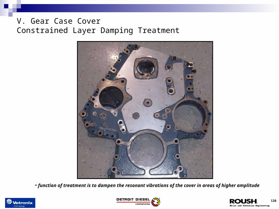
V. Gear Case CoverConstrained Layer Damping Treatment
-function of treatment is to dampen the resonant vibrations of the cover in areas of higher amplitude

127
V. Acoustically Treated Oil Pan
-acoustical barrier intended to reduce amount of radiated noise emitted from oil pan surfaces-preliminary results show a reduction of 2 dBA in passby noise compared to production oil pan

128
V. Bedplate Block Stiffener
-bedplate is intended to stiffen crankcase to reduce structural vibration and shift natural frequencies out of normal operating engine frequency range (> 200 Hz)


130
VI. N&V Sensors
A. Accelerometers
B. Microphones
C. Rotational speed transducers
D. Transducer calibration
131
VI.A. Accelerometers
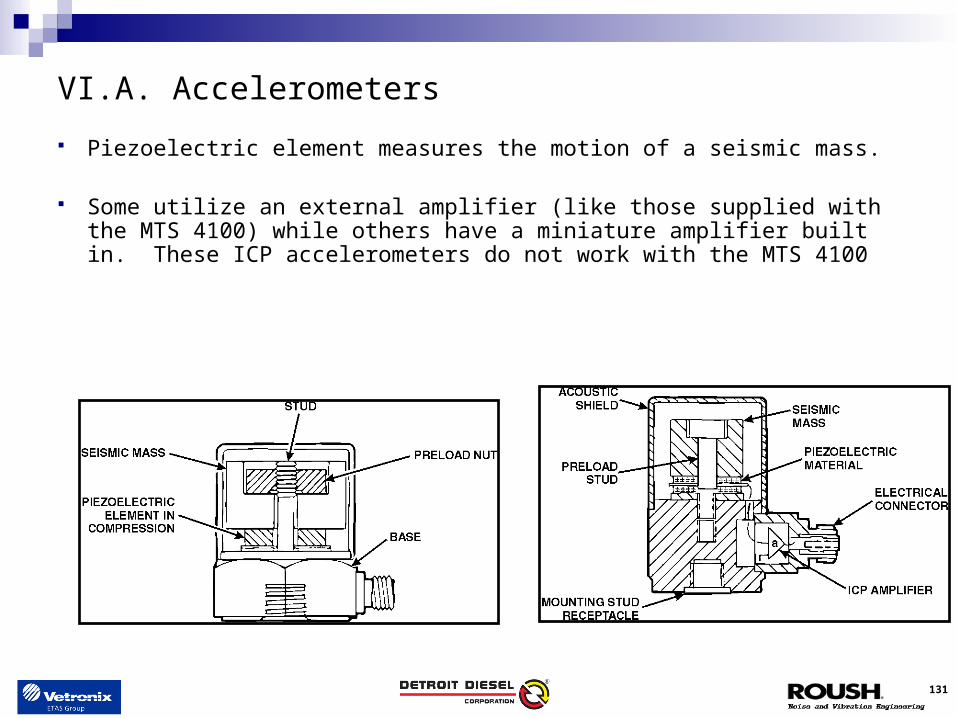
Piezoelectric element measures the motion of a seismic mass.
Some utilize an external amplifier (like those supplied with the MTS 4100) while others have a miniature amplifier built in. These ICP accelerometers do not work with the MTS 4100

132
VI.A. Accelerometers
Accelerometers may be either longitudinal or shear type.
133
VI.B. Microphones
The DDC MTS 4100 kit contains a microphone. The microphone has a piezoelectric sensing element, and it uses an ICP (Integrated Circuit Power) conditioning unit. This type of microphone is very durable and temperature resistant.
The piezoelectric element produces an electrical charge proportional to the applied acoustic pressure. This charge is amplified by a small circuit (called a preamp) located near the piezoelectric element. The preamp circuit is powered by a DC voltage that is carried over the same wires as the signal between the signal conditioner and the preamp. The signal conditioner supplies the DC voltage (ICP) and separates the AC signal from the DC voltage using a high pass filter.
Other types of microphones (including condenser microphones, dynamic microphones, and crystal microphones) are available from local sources. These all have different signal conditioning and impedance matching requirements, and they might not be compatible with the MTS 4100.

134
VI.C. Rotational Speed Transducers
DDC N&V engineers measure torsional vibrations by mounting a toothed gear and using a magnetic pickup (mag-probe) to produce a pulse every time a tooth passes the probe.
The data is processed by examining the frequency fluctuation of the signal – the frequency modulation (FM). The MTS 4100 analyzer does not currently support this function.
135
VI.C. Transducer Calibration
Calibration values are provided for the accelerometers and microphone provided with the MTS 4100. These are entered using the procedures in the next major section of the course. (for example, Setup Menu>Calibrate Sensors>Microphone A – sensitivity)
For microphones and accelerometers, standard calibrators are available so that the transducer calibration can be checked before and after each use. These are not included in the MTS 4100 kit.
Depending on company ISO requirements, the MTS 4100 and its transducers should be returned to ETAS periodically for calibration. Probably once per year.


137
Quiz
1. The MTS 4100 and almost all analyzers calculate the frequency spectrum (magnitude vs frequency) using:
A. Fourier Transform
B. Discrete Fourier Transform (DFT)
C. Fast Fourier Transform (FFT)
D. Third-Octave Band Analyzer
2. Based on the single degree of freedom (SDOF) model, what property has the strongest effect on the amplitude of vibration at the natural frequency:
A. Mass
B. Stiffness
C. Damping

138
Quiz
3. The dynamic behavior of which of the following physical systems can be better understood using the SDOF model:
A. Engine on mounts
B. Cab on mounts
C. Steering column
D. Exhaust system
E. Acoustic modes of cab
F. Rear cab panel
G. A and B because the model is only useful for rigid body modes
H. All of the above

139
Quiz
4. Based on the single degree of freedom (SDOF) model, mount isolation is best:A. Below the natural frequencyB. Above the natural frequencyC. At the natural frequency
5. Which of the following is NOT a source of vibration per the source/path/receiver modelA. Resonance of the exhaust systemB. Engine vibrationC. Road inputs to the suspensionD. Driveline imbalanceE. Tire force variationF. Wind noise

140
Quiz
6. Why is noise data A-weighted:
A. To correct for the change in the speed-of-sound due to varying air temperature/density.
B. To approximately mimic the frequency sensitivity of the human ear so that measured sound levels correlate to perceived sound levels.
C. To approximately mimic the change in frequency sensitivity of the human ear as loudness changes.
7. Which increase in noise level is perceived as twice as loud:
A. 40 dBA to 50 dBA
B. 40 dBA to 80 dBA
C. 40 dBA to 46 dBA
141
Quiz
8. The difference between barely perceivable sound and painful sound is 3 million times. The difference between barely perceivable and intolerable vibration is:
A. 3 million times
B. 10 times
C. Approximately 100 times
9. The Series 60 engine is a six cylinder engine with even firing intervals. What is the order of the engine firing frequency:
A. 6th order
B. 3rd order
C. 1st order
142
Quiz
True or false:
10. Driveline angles don’t matter because the Cardan Joint is flexible.
11. In the Campbell Diagram, resonances are lines at a particular frequency.
12. In the Campbell Diagram, orders are lines at a particular frequency.
13. Critical speed is the nominal design condition for a rotating shaft.
14. The MTS 4100 reads vehicle speed information from the computer bus to calculate driveline rotation speed.
15. Cardan joints produce 2nd order driveline vibration.
16. Driveline imbalance produces 2nd order driveline vibration.
143
Quiz Answers
1C. The FFT is used to calculate the frequency spectrum due to its computational speed.
2C. While the mass and stiffness determine the natural frequency, the amplitude is determined by the damping.
3H. All dynamical systems that are approximately linear can be better understood using the SDOF model. All these systems have natural frequencies with associated mass, spring, and damping properties.
4B. Isolation is best above the natural frequency. As the frequency approaches zero, the isolation is one. At the natural frequency, there is gain (for lightly damped systems which are most common), so the isolation is poor.
5A. Resonance of the exhaust system is a path issue, all the others are sources of vehicle vibration.
6B. A-weighting corrects for the frequency response of human hearing at lower sound levels. B-weighting corrects for intermediate sound levels, and C-weighting corrects for high sound levels.
144
Quiz Answers
7A. An increase in loudness of 10 dBA is perceived as twice as loud. An increase of 6 dBA corresponds to a doubling of sound pressure. Increasing the sound level by 40 dBA would be perceived as being 16 times louder (= 2x2x2x2).
8C. The difference between barely perceivable and intolerable vibration is approximately 100 times. Vibration perception is approximately linear, while sound perception is compressed logarithmically.
9B. A single-cylinder, four-stroke engine has a firing order of ½ because the cycle of intake-compression-combustion-exhaust takes two revolutions to complete. This process takes place six times faster for a six cylinder engine with even firing intervals, so the order of the firing frequency is 3rd order (= 0.5*6).
10.F 11.T 12.F 13.F 14.T 15.T 16.F