Basic Statistics and Probability Theory

Based on

“Foundations of Statistical NLP”

C. Manning & H. Schutze, ch. 2, MIT Press, 2002

“Probability theory is nothing but common sense

reduced to calculation.”

Pierre Simon, Marquis de Laplace (1749-1827)

0.

PLAN

1. Elementary Probability Notions:• Sample Space, Event Space, and Probability Function

• Conditional Probability

• Bayes’ Theorem

• Independence of Probabilistic Events

2. Random Variables:

• Discrete Variables and Continuous Variables

• Mean, Variance and Standard Deviation

• Standard Distributions

• Joint, Marginal and and Conditional Distributions

• Independence of Random Variables

1.

PLAN (cont’d)

3. Limit Theorems

• Laws of Large Numbers

• Central Limit Theorems

4. Estimating the parameters of probabilistic models fromdata

• Maximum Likelihood Estimation (MLE)

• Maximum A Posteriori (MAP) Estimation

5. Elementary Information Theory

• Entropy; Conditional Entropy; Joint Entropy

• Information Gain / Mutual Information

• Cross-Entropy

• Relative Entropy / Kullback-Leibler (KL) Divergence

• Properties: bounds, chain rules, (non-)symmetries,properties pertaining to independence

2.

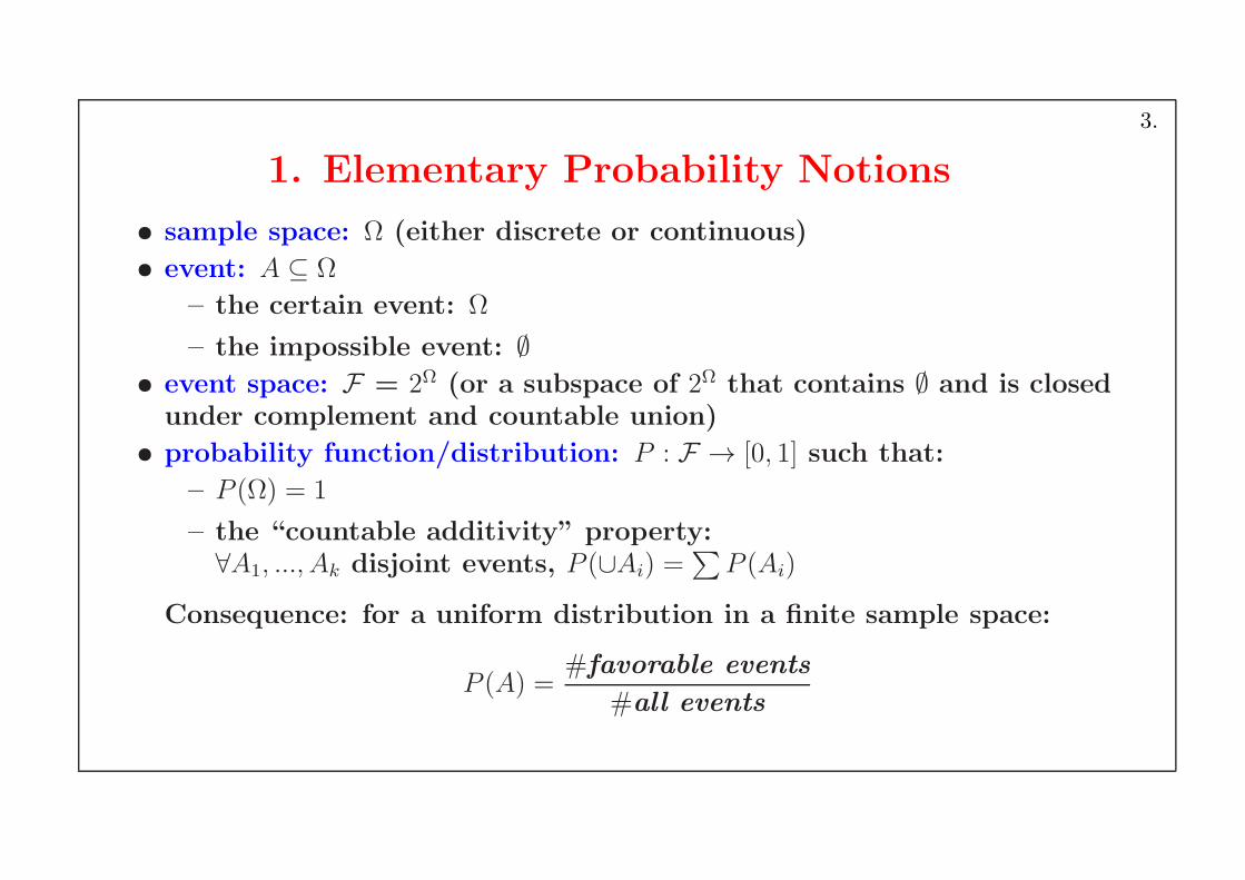
1. Elementary Probability Notions

• sample space: Ω (either discrete or continuous)

• event: A ⊆ Ω

– the certain event: Ω

– the impossible event: ∅• event space: F = 2Ω (or a subspace of 2Ω that contains ∅ and is closedunder complement and countable union)

• probability function/distribution: P : F → [0, 1] such that:

– P (Ω) = 1

– the “countable additivity” property:∀A1, ..., Ak disjoint events, P (∪Ai) =

∑

P (Ai)

Consequence: for a uniform distribution in a finite sample space:

P (A) =#favorable events

#all events

3.

Conditional Probability

• P (A | B) =P (A ∩B)P (B)

Note: P (A | B) is called the a posteriory probability of A, given B.

• The “multiplication” rule:

P (A ∩B) = P (A | B)P (B) = P (B | A)P (A)

• The “chain” rule:

P (A1 ∩ A2 ∩ . . . ∩ An) =P (A1)P (A2 | A1)P (A3 | A1, A2) . . . P (An | A1, A2, . . . , An−1)

4.

• The “total probability” formula:

P (A) = P (A | B)P (B) + P (A | ¬B)P (¬B)

More generally:

if A ⊆ ∪Bi and ∀i 6= j Bi ∩Bj = ∅, thenP (A) =

∑

i P (A | Bi)P (Bi)

• Bayes’ Theorem:

P (B | A) =P (A | B) P (B)

P (A)

or P (B | A) =P (A | B) P (B)

P (A | B)P (B) + P (A | ¬B)P (¬B)

or ...

5.

Independence of Probabilistic Events

• Independent events: P (A ∩ B) = P (A)P (B)

Note: When P (B) 6= 0, the above definition is equivalent toP (A|B) = P (A).

• Conditionally independent events:P (A ∩ B | C) = P (A | C)P (B | C), assuming, of course, thatP (C) 6= 0.

Note: When P (B ∩ C) 6= 0, the above definition is equivalentto P (A|B,C) = P (A|C).

6.

2. Random Variables

2.1 Basic Definitions

Let Ω be a sample space, andP : 2Ω → [0, 1] a probability function.

• A random variable of distribution P is a function

X : Ω → Rn

For now, let us consider n = 1.

The cumulative distribution function of X is F : R → [0,∞) defined by

F (x) = P (X ≤ x) = P (ω ∈ Ω | X(ω) ≤ x)

7.

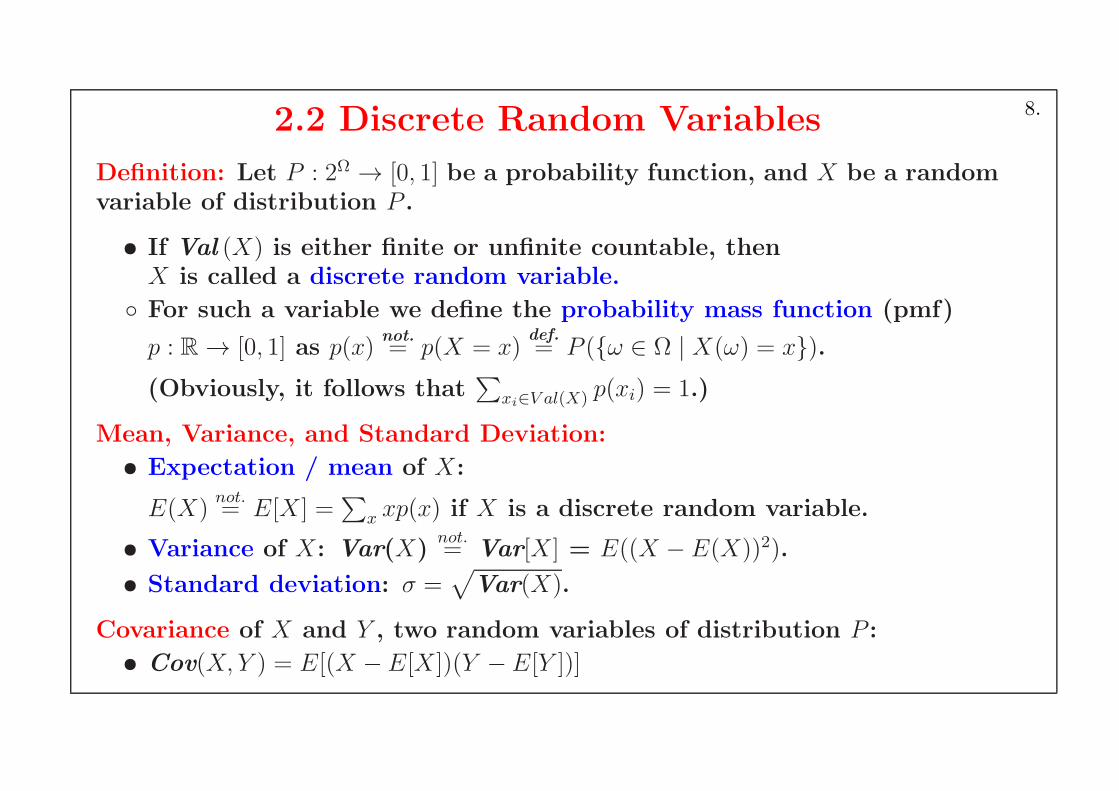
2.2 Discrete Random Variables

Definition: Let P : 2Ω → [0, 1] be a probability function, and X be a randomvariable of distribution P .

• If Val (X) is either finite or unfinite countable, thenX is called a discrete random variable.

For such a variable we define the probability mass function (pmf)

p : R → [0, 1] as p(x)not.= p(X = x)

def.= P (ω ∈ Ω | X(ω) = x).

(Obviously, it follows that∑

xi∈V al(X) p(xi) = 1.)

Mean, Variance, and Standard Deviation:

• Expectation / mean of X:

E(X)not.= E[X ] =

∑

x xp(x) if X is a discrete random variable.

• Variance of X: Var(X)not.= Var[X ] = E((X − E(X))2).

• Standard deviation: σ =√

Var(X).

Covariance of X and Y , two random variables of distribution P :

• Cov(X, Y ) = E[(X −E[X ])(Y −E[Y ])]

8.

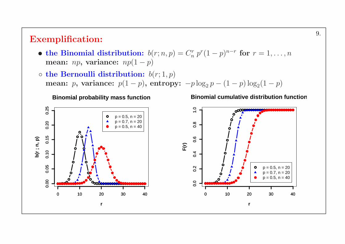
Exemplification:

• the Binomial distribution: b(r;n, p) = Crn pr(1− p)n−r for r = 1, . . . , n

mean: np, variance: np(1− p)

the Bernoulli distribution: b(r; 1, p)mean: p, variance: p(1− p), entropy: −p log2 p− (1− p) log2(1− p)

0 10 20 30 40

0.00

0.05

0.10

0.15

0.20

0.25

r

b(r

; n

, p)

0 10 20 30 40

0.00

0.05

0.10

0.15

0.20

0.25

Binomial probability mass function

p = 0.5, n = 20p = 0.7, n = 20p = 0.5, n = 40

0 10 20 30 400.

00.

20.

40.

60.

81.

0

r

F(r

)

0 10 20 30 400.

00.

20.

40.

60.

81.

0

Binomial cumulative distribution function

p = 0.5, n = 20p = 0.7, n = 20p = 0.5, n = 40

9.

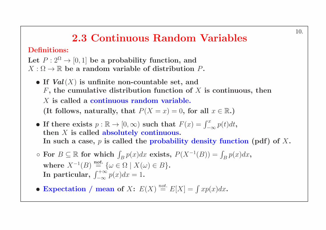
2.3 Continuous Random VariablesDefinitions:

Let P : 2Ω → [0, 1] be a probability function, andX : Ω → R be a random variable of distribution P .

• If Val (X) is unfinite non-countable set, andF , the cumulative distribution function of X is continuous, then

X is called a continuous random variable.

(It follows, naturally, that P (X = x) = 0, for all x ∈ R.)

• If there exists p : R → [0,∞) such that F (x) =∫ x

−∞p(t)dt,

then X is called absolutely continuous.In such a case, p is called the probability density function (pdf) of X.

For B ⊆ R for which∫

Bp(x)dx exists, P (X−1(B)) =

∫

Bp(x)dx,

where X−1(B)not.= ω ∈ Ω | X(ω) ∈ B.

In particular,∫ +∞

−∞p(x)dx = 1.

• Expectation / mean of X: E(X)not.= E[X ] =

∫

xp(x)dx.

10.

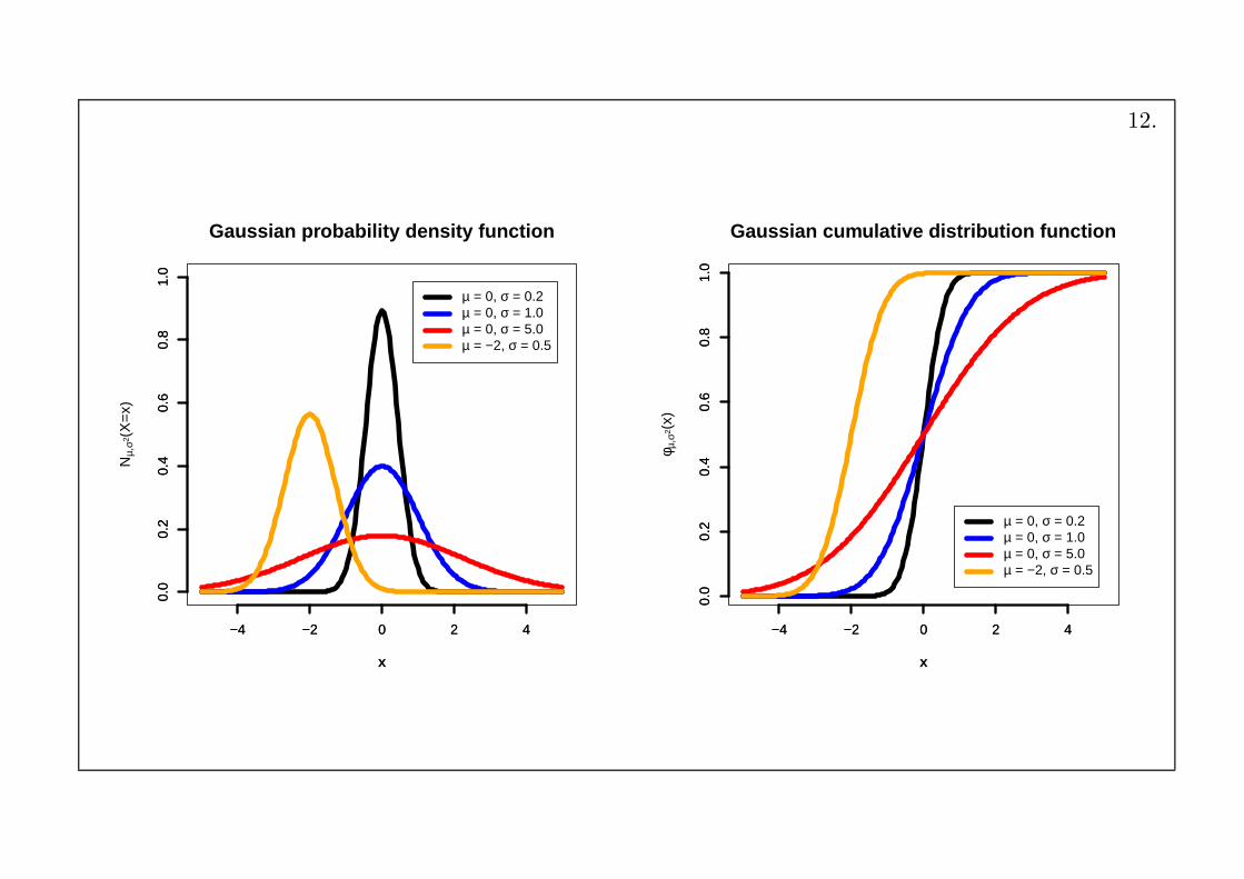
Exemplification:

• Normal (Gaussean) distribution: N(x;µ, σ) = 1√2πσ

e−(x− µ)2

2σ2

mean: µ, variance: σ2

Standard Normal distribution: N(x; 0, 1)

• Remark:

For n, p such that np(1 − p) > 5, the Binomial distributions can beapproximated by Normal distributions.

11.

−4 −2 0 2 4

0.0

0.2

0.4

0.6

0.8

1.0

x

Nµ,

σ2 (X

=x)

−4 −2 0 2 4

0.0

0.2

0.4

0.6

0.8

1.0

Gaussian probability density function

µ = 0, σ = 0.2µ = 0, σ = 1.0µ = 0, σ = 5.0µ = −2, σ = 0.5

−4 −2 0 2 4

0.0

0.2

0.4

0.6

0.8

1.0

xφ µ

,σ2 (

x)

−4 −2 0 2 4

0.0

0.2

0.4

0.6

0.8

1.0

Gaussian cumulative distribution function

µ = 0, σ = 0.2µ = 0, σ = 1.0µ = 0, σ = 5.0µ = −2, σ = 0.5

12.

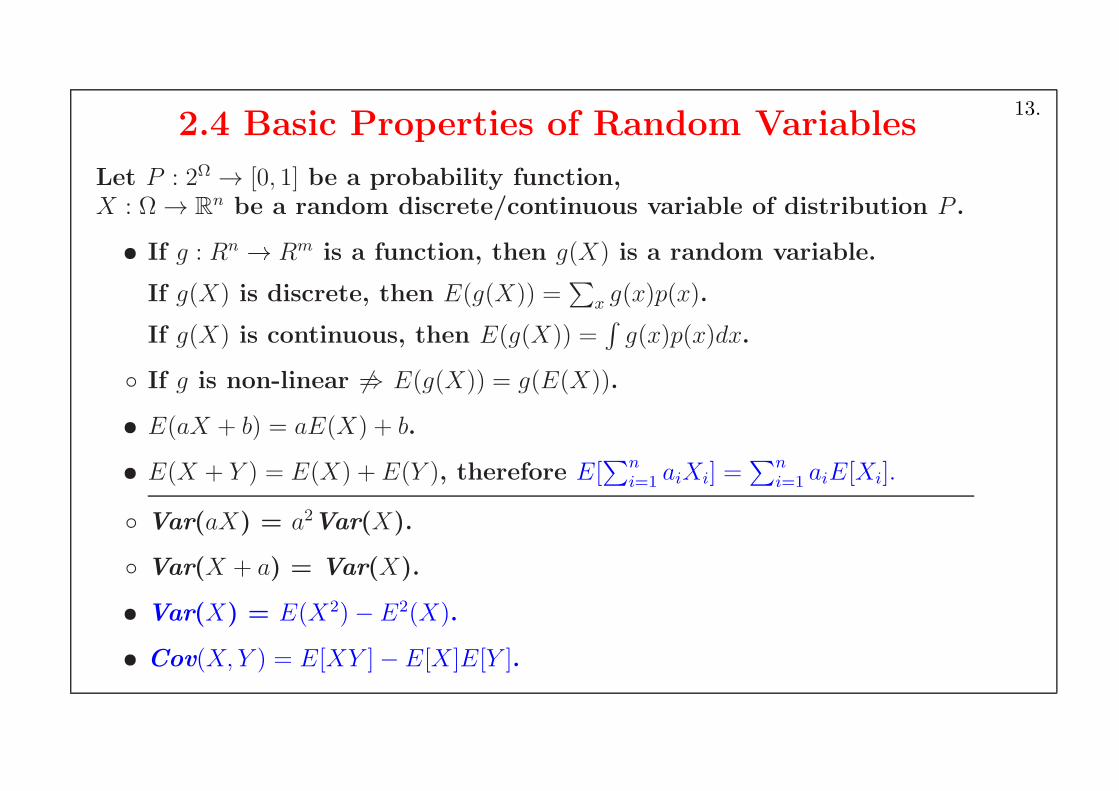
2.4 Basic Properties of Random Variables

Let P : 2Ω → [0, 1] be a probability function,X : Ω → R

n be a random discrete/continuous variable of distribution P .

• If g : Rn → Rm is a function, then g(X) is a random variable.

If g(X) is discrete, then E(g(X)) =∑

x g(x)p(x).

If g(X) is continuous, then E(g(X)) =∫

g(x)p(x)dx.

If g is non-linear 6⇒ E(g(X)) = g(E(X)).

• E(aX + b) = aE(X) + b.

• E(X + Y ) = E(X) + E(Y ), therefore E[∑n

i=1 aiXi] =∑n

i=1 aiE[Xi].

Var(aX) = a2Var(X).

Var(X + a) = Var(X).

• Var(X) = E(X2)− E2(X).

• Cov(X, Y ) = E[XY ]− E[X ]E[Y ].

13.

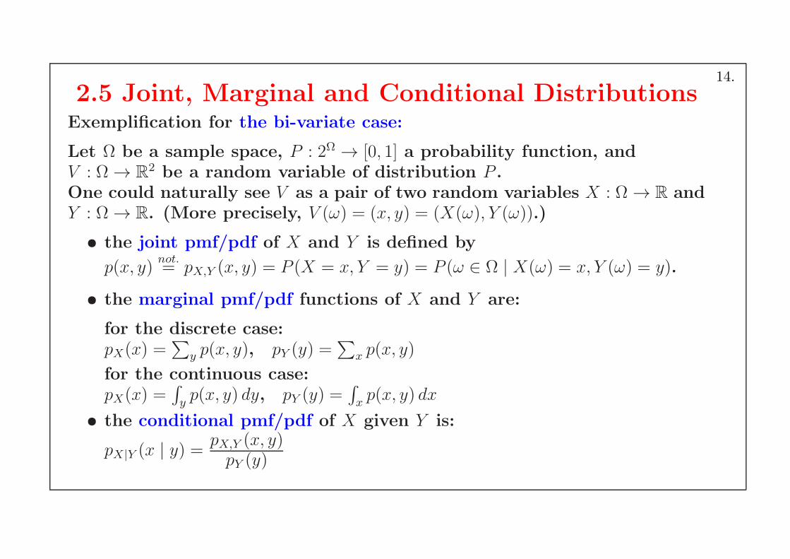
2.5 Joint, Marginal and Conditional DistributionsExemplification for the bi-variate case:

Let Ω be a sample space, P : 2Ω → [0, 1] a probability function, andV : Ω → R

2 be a random variable of distribution P .One could naturally see V as a pair of two random variables X : Ω → R andY : Ω → R. (More precisely, V (ω) = (x, y) = (X(ω), Y (ω)).)

• the joint pmf/pdf of X and Y is defined by

p(x, y)not.= pX,Y (x, y) = P (X = x, Y = y) = P (ω ∈ Ω | X(ω) = x, Y (ω) = y).

• the marginal pmf/pdf functions of X and Y are:

for the discrete case:pX(x) =

∑

y p(x, y), pY (y) =∑

x p(x, y)

for the continuous case:pX(x) =

∫

yp(x, y) dy, pY (y) =

∫

xp(x, y) dx

• the conditional pmf/pdf of X given Y is:

pX|Y (x | y) = pX,Y (x, y)pY (y)

14.

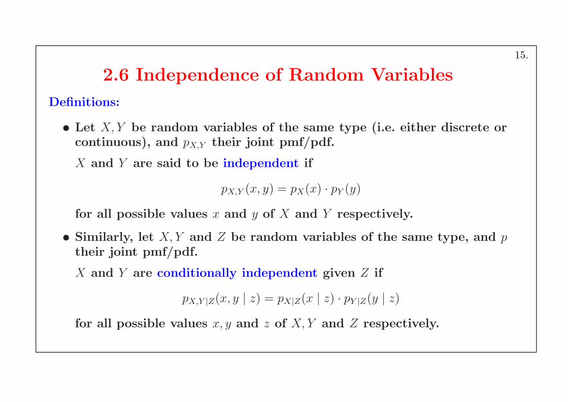
2.6 Independence of Random Variables

Definitions:

• Let X, Y be random variables of the same type (i.e. either discrete orcontinuous), and pX,Y their joint pmf/pdf.

X and Y are said to be independent if

pX,Y (x, y) = pX(x) · pY (y)

for all possible values x and y of X and Y respectively.

• Similarly, let X, Y and Z be random variables of the same type, and ptheir joint pmf/pdf.

X and Y are conditionally independent given Z if

pX,Y |Z(x, y | z) = pX|Z(x | z) · pY |Z(y | z)

for all possible values x, y and z of X, Y and Z respectively.

15.

Properties of random variables pertaining to independence

• If X, Y are independent, thenVar(X + Y ) = Var(X) + Var(Y ).

• If X, Y are independent, thenE(XY ) = E(X)E(Y ), i.e. Cov(X, Y ) = 0.

Cov(X, Y ) = 0 6⇒ X, Y are independent.

The covariance matrix corresponding to a vector of random variablesis symmetric and positive semi-definite.

• If the covariance matrix of a multi-variate Gaussian distribution isdiagonal, then the marginal distributions are independent.

16.

3. Limit Theorems[ Sheldon Ross, A first course in probability, 5th ed., 1998 ]

“The most important results in probability theory are limit theo-rems. Of these, the most important are...

laws of large numbers, concerned with stating conditions underwhich the average of a sequence of random variables converges (insome sense) to the expected average;

central limit theorems, concerned with determining the conditionsunder which the sum of a large number of random variables has aprobability distribution that is approximately normal.”

17.

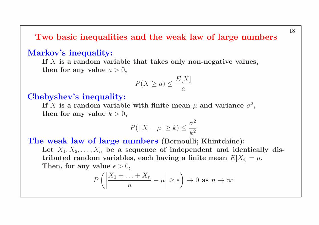
Two basic inequalities and the weak law of large numbers

Markov’s inequality:If X is a random variable that takes only non-negative values,then for any value a > 0,

P (X ≥ a) ≤ E[X ]

aChebyshev’s inequality:

If X is a random variable with finite mean µ and variance σ2,then for any value k > 0,

P (| X − µ |≥ k) ≤ σ2

k2

The weak law of large numbers (Bernoulli; Khintchine):Let X1, X2, . . . , Xn be a sequence of independent and identically dis-tributed random variables, each having a finite mean E[Xi] = µ.Then, for any value ǫ > 0,

P

(∣

∣

∣

∣

X1 + . . .+Xn

n− µ

∣

∣

∣

∣

≥ ǫ

)

→ 0 as n → ∞

18.

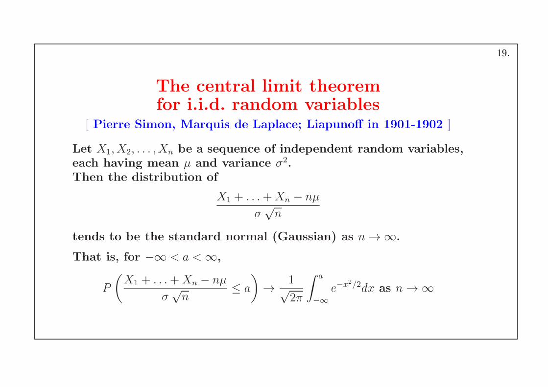
The central limit theoremfor i.i.d. random variables

[ Pierre Simon, Marquis de Laplace; Liapunoff in 1901-1902 ]

Let X1, X2, . . . , Xn be a sequence of independent random variables,each having mean µ and variance σ2.Then the distribution of

X1 + . . .+Xn − nµ

σ√n

tends to be the standard normal (Gaussian) as n → ∞.

That is, for −∞ < a < ∞,

P

(

X1 + . . .+Xn − nµ

σ√n

≤ a

)

→ 1√2π

∫ a

−∞

e−x2/2dx as n → ∞

19.

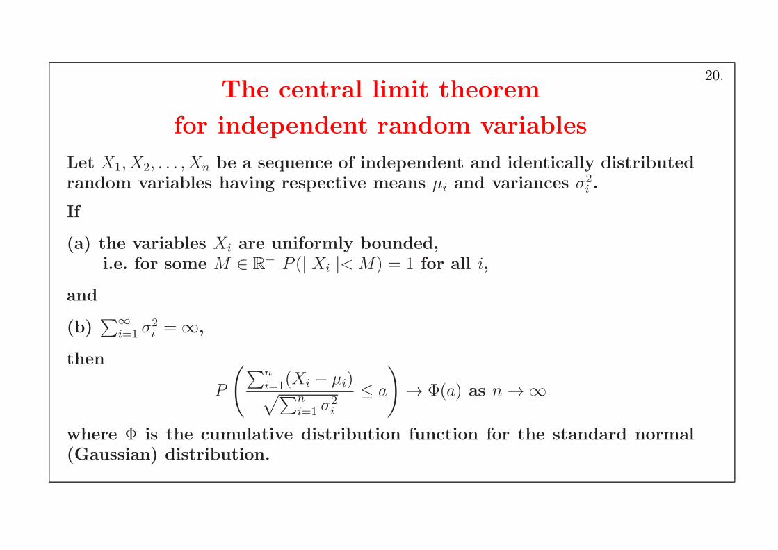
The central limit theorem

for independent random variables

Let X1, X2, . . . , Xn be a sequence of independent and identically distributedrandom variables having respective means µi and variances σ2

i .

If

(a) the variables Xi are uniformly bounded,i.e. for some M ∈ R

+ P (| Xi |< M) = 1 for all i,

and

(b)∑∞

i=1 σ2i = ∞,

then

P

(

∑ni=1(Xi − µi)√

∑ni=1 σ

2i

≤ a

)

→ Φ(a) as n → ∞

where Φ is the cumulative distribution function for the standard normal(Gaussian) distribution.

20.

The strong law of large numbers

Let X1, X2, . . . , Xn be a sequence of independent and identicallydistributed random variables, each having a finite mean E[Xi] = µ.Then, with probability 1,

X1 + . . .+Xn

n→ µ as n → ∞

That is,

P(

limn→∞

(X1 + . . .+Xn)/n = µ)

= 1

21.

Other inequalitiesOne-sided Chebyshev inequality:

If X is a random variable with mean 0 and finite variance σ2,then for any a > 0,

P (X ≥ a) ≤ σ2

σ2 + a2

Corollary:

If E[X ] = µ, Var(X) = σ2, then for a > 0

P (X ≥ µ+ a) ≤ σ2

σ2 + a2

P (X ≤ µ− a) ≤ σ2

σ2 + a2

Chernoff bounds:

Let M(t)not= E[etX ]. Then

P (X ≥ a) ≤ e−taM(t) for all t > 0

P (X ≥ a) ≤ e−taM(t) for all t < 0

22.

4. Estimation/inference of the parameters ofprobabilistic models from data

(based on [Durbin et al, Biological Sequence Analysis, 1998],p. 311-313, 319-321)

A probabilistic model can be anything from a simple distributionto a complex stochastic grammar with many implicit probabilitydistributions. Once the type of the model is chosen, the parame-ters have to be inferred from data.

We will first consider the case of the categorical distribution, andthen we will present the different strategies that can be used ingeneral.

23.

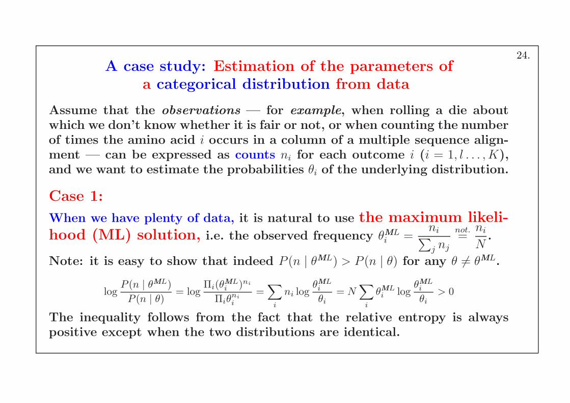
A case study: Estimation of the parameters ofa categorical distribution from data

Assume that the observations — for example, when rolling a die aboutwhich we don’t know whether it is fair or not, or when counting the numberof times the amino acid i occurs in a column of a multiple sequence align-ment — can be expressed as counts ni for each outcome i (i = 1, l . . . , K),and we want to estimate the probabilities θi of the underlying distribution.

Case 1:

When we have plenty of data, it is natural to use the maximum likeli-hood (ML) solution, i.e. the observed frequency θML

i =ni

∑

j nj

not.=

ni

N.

Note: it is easy to show that indeed P (n | θML) > P (n | θ) for any θ 6= θML.

logP (n | θML)

P (n | θ) = logΠi(θ

MLi )ni

Πiθni

i

=∑

i

ni logθMLi

θi= N

∑

i

θMLi log

θMLi

θi> 0

The inequality follows from the fact that the relative entropy is alwayspositive except when the two distributions are identical.

24.

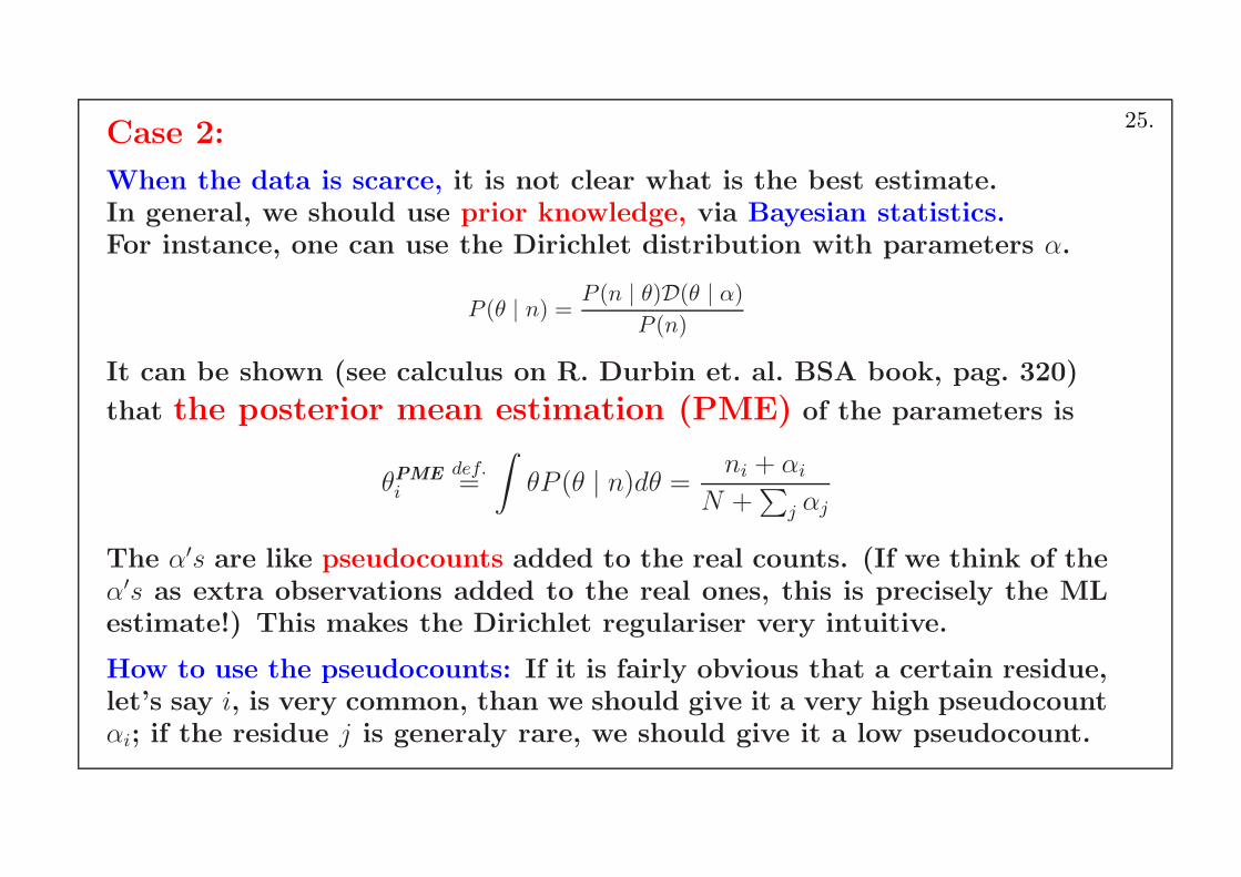
Case 2:

When the data is scarce, it is not clear what is the best estimate.In general, we should use prior knowledge, via Bayesian statistics.For instance, one can use the Dirichlet distribution with parameters α.

P (θ | n) = P (n | θ)D(θ | α)P (n)

It can be shown (see calculus on R. Durbin et. al. BSA book, pag. 320)

that the posterior mean estimation (PME) of the parameters is

θPMEi

def.=

∫

θP (θ | n)dθ =ni + αi

N +∑

j αj

The α′s are like pseudocounts added to the real counts. (If we think of theα′s as extra observations added to the real ones, this is precisely the MLestimate!) This makes the Dirichlet regulariser very intuitive.

How to use the pseudocounts: If it is fairly obvious that a certain residue,let’s say i, is very common, than we should give it a very high pseudocountαi; if the residue j is generaly rare, we should give it a low pseudocount.

25.

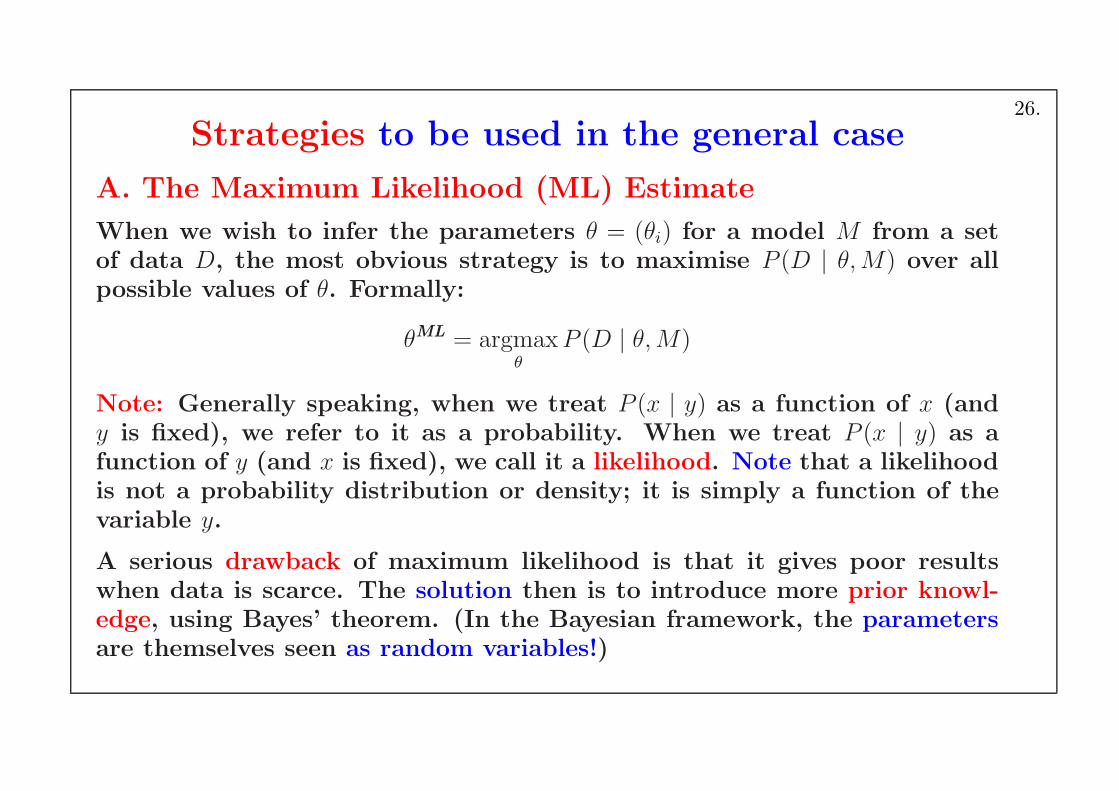
Strategies to be used in the general case

A. The Maximum Likelihood (ML) Estimate

When we wish to infer the parameters θ = (θi) for a model M from a setof data D, the most obvious strategy is to maximise P (D | θ,M) over allpossible values of θ. Formally:

θML = argmaxθ

P (D | θ,M)

Note: Generally speaking, when we treat P (x | y) as a function of x (andy is fixed), we refer to it as a probability. When we treat P (x | y) as afunction of y (and x is fixed), we call it a likelihood. Note that a likelihoodis not a probability distribution or density; it is simply a function of thevariable y.

A serious drawback of maximum likelihood is that it gives poor resultswhen data is scarce. The solution then is to introduce more prior knowl-edge, using Bayes’ theorem. (In the Bayesian framework, the parametersare themselves seen as random variables!)

26.

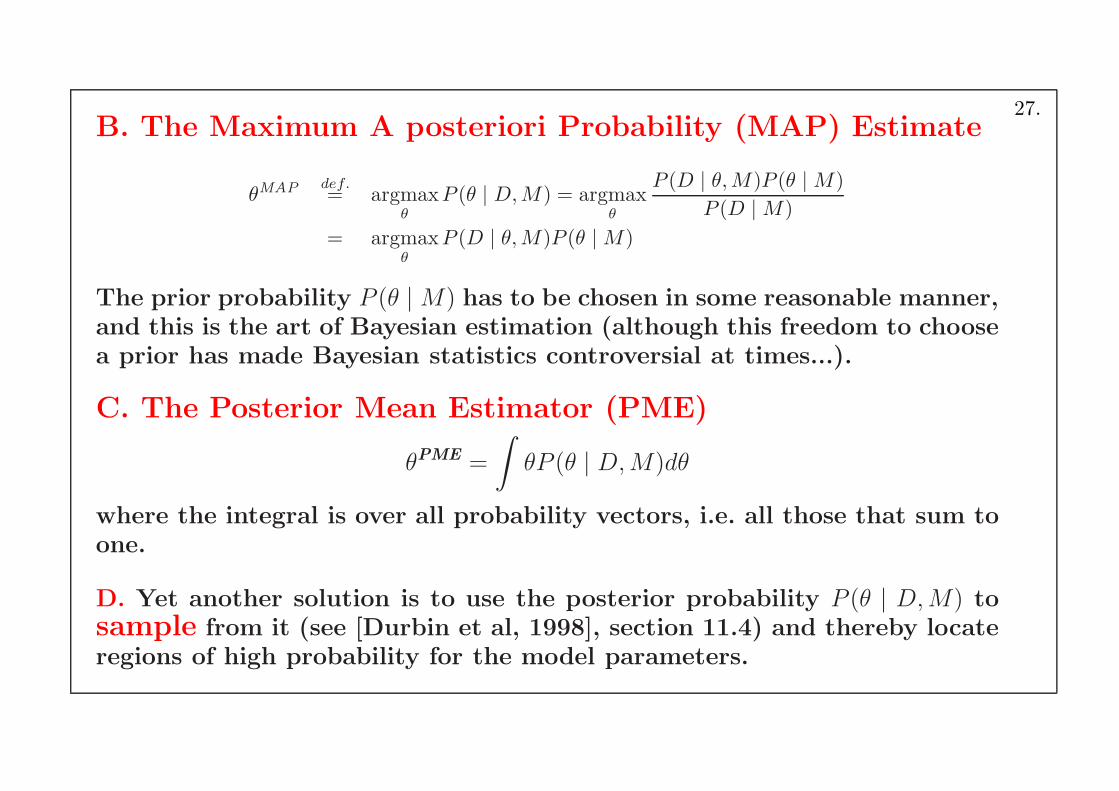
B. The Maximum A posteriori Probability (MAP) Estimate

θMAP def.= argmax

θP (θ | D,M) = argmax

θ

P (D | θ,M)P (θ | M)

P (D | M)

= argmaxθ

P (D | θ,M)P (θ | M)

The prior probability P (θ | M) has to be chosen in some reasonable manner,and this is the art of Bayesian estimation (although this freedom to choosea prior has made Bayesian statistics controversial at times...).

C. The Posterior Mean Estimator (PME)

θPME =

∫

θP (θ | D,M)dθ

where the integral is over all probability vectors, i.e. all those that sum toone.

D. Yet another solution is to use the posterior probability P (θ | D,M) tosample from it (see [Durbin et al, 1998], section 11.4) and thereby locateregions of high probability for the model parameters.

27.

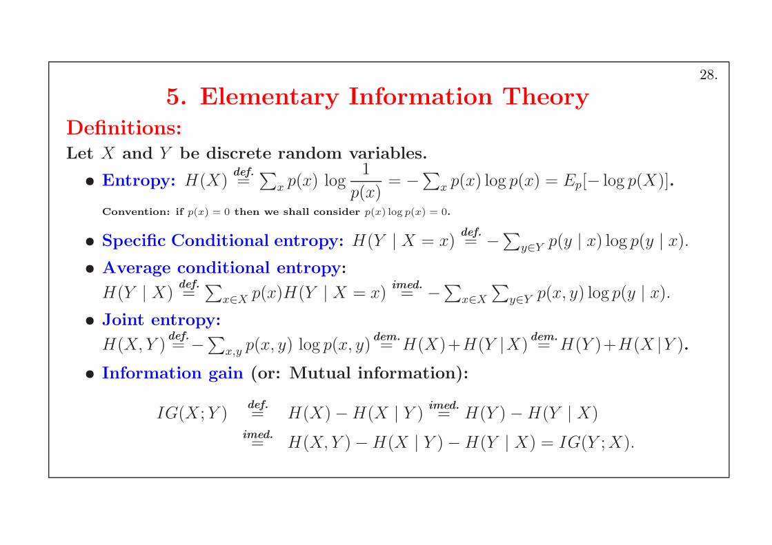
5. Elementary Information TheoryDefinitions:Let X and Y be discrete random variables.

• Entropy: H(X)def.=∑

x p(x) log1

p(x)= −∑x p(x) log p(x) = Ep[− log p(X)].

Convention: if p(x) = 0 then we shall consider p(x) log p(x) = 0.

• Specific Conditional entropy: H(Y | X = x)def.= −∑y∈Y p(y | x) log p(y | x).

• Average conditional entropy:

H(Y | X)def.=∑

x∈X p(x)H(Y | X = x)imed.= −∑x∈X

∑

y∈Y p(x, y) log p(y | x).• Joint entropy:

H(X, Y )def.= −∑x,y p(x, y) log p(x, y)

dem.= H(X)+H(Y |X)

dem.= H(Y )+H(X |Y ).

• Information gain (or: Mutual information):

IG(X ; Y )def.= H(X)−H(X | Y )

imed.= H(Y )−H(Y | X)

imed.= H(X, Y )−H(X | Y )−H(Y | X) = IG(Y ;X).

28.

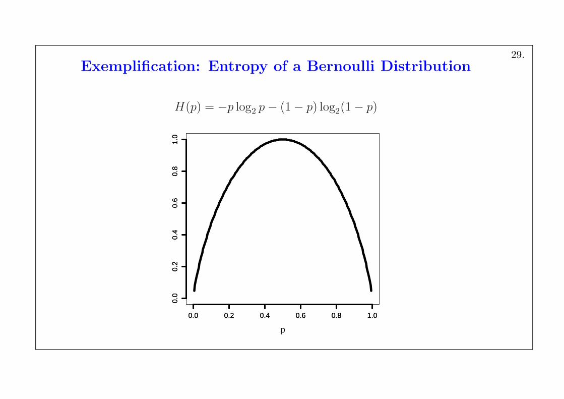
Exemplification: Entropy of a Bernoulli Distribution

H(p) = −p log2 p− (1− p) log2(1− p)

0.0 0.2 0.4 0.6 0.8 1.0

0.0

0.2

0.4

0.6

0.8

1.0

p

0.0 0.2 0.4 0.6 0.8 1.0

0.0

0.2

0.4

0.6

0.8

1.0

29.

Basic properties of

Entropy, Conditional Entropy, Joint Entropy and

Information Gain / Mutual Information

• 0 ≤ H(p1, . . . , pn) ≤ H

(

1

n, . . . ,

1

n

)

= log n;

H(X) = 0 iff X is a constant random variable.

• IG(X ; Y ) ≥ 0;IG(X ; Y ) = 0 iff X and Y are independent.

• H(X | Y ) ≤ H(X)H(X | Y ) = H(X) iff X and Y are independent;

H(X, Y ) ≤ H(X) +H(Y );H(X, Y ) = H(X) +H(Y ) iff X and Y are independent.

• a chain rule: H(X1, . . . , Xn) = H(X1)+H(X2|X1)+. . .+H(Xn|X1, . . . , Xn−1).

30.

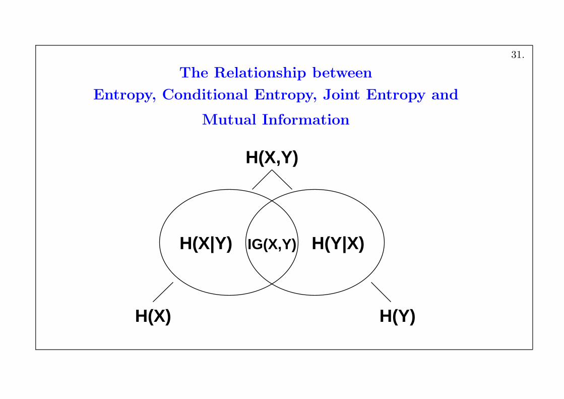
The Relationship between

Entropy, Conditional Entropy, Joint Entropy and

Mutual Information

H(X|Y) H(Y|X)

H(X,Y)

H(X) H(Y)

IG(X,Y)

31.

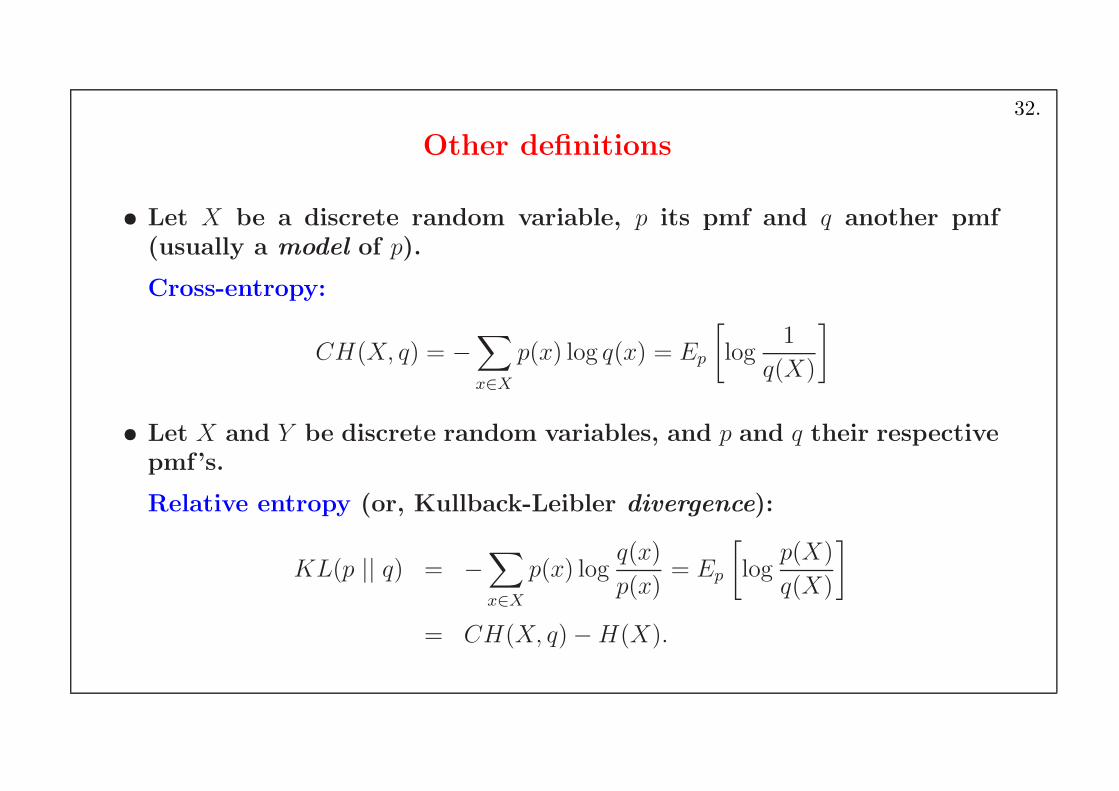
Other definitions

• Let X be a discrete random variable, p its pmf and q another pmf(usually a model of p).

Cross-entropy:

CH(X, q) = −∑

x∈X

p(x) log q(x) = Ep

[

log1

q(X)

]

• Let X and Y be discrete random variables, and p and q their respectivepmf’s.

Relative entropy (or, Kullback-Leibler divergence):

KL(p || q) = −∑

x∈X

p(x) logq(x)

p(x)= Ep

[

logp(X)

q(X)

]

= CH(X, q)−H(X).

32.

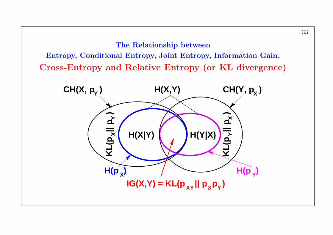
The Relationship between

Entropy, Conditional Entropy, Joint Entropy, Information Gain,

Cross-Entropy and Relative Entropy (or KL divergence)

XH(p )

CH(X, p )Y CH(Y, p )X

XK

L(p

|| p

) Y

YH(p )

YK

L(p

|| p

) X

H(X|Y) H(Y|X)

H(X,Y)

YXY XIG(X,Y) = KL(p || p p )

33.

Basic properties ofcross-entropy and relative entropy

CH(X, q) ≥ 0

• KL(p || q) ≥ 0 for all p and q;KL(p || q) = 0 iff p and q are identical.

[Consequence:]If X is a discrete random variable, p its pmf, and q another pmf,then CH(X, q) ≥ H(X) ≥ 0.

The first of these two inequations is also known as Gibbs’ inequation:−∑n

i=1 pi log2 pi ≤ −∑i pi log2 qi.

Unlike H of a discrete n-ary variable, which is bounded by log2 n, thereis no (general) upper bound for CH. (However, KL is upper-bounded.)

• Unlike H(X, Y ), which is symmetric in its arguments, CH and KL arenot! Therefore KL is NOT a distance metric! (See the next slide.)

• IG(X ; Y ) = KL(pXY || pX pY ) =∑

x

∑

y p(x, y) log

(

p(x)p(y)

p(x, y)

)

.

34.

Remark

The quantity

V I(X, Y )def= H(X, Y )− IG(X ; Y ) = H(X) +H(Y )− 2IG(X ; Y )

= H(X | Y ) +H(Y | X)

known as variation of information, is a distance metric, i.e. it isnonengative, symmetric, implies indiscernability, and satisfies the tri-angle inequality.

Consider M(p, q) =1

2(p+ q).

The function JSD(p||q) = 1

2KL(p||M) +

1

2KL(q||M) is called the Jensen-

Shannon divergence.

One can prove that√

JSD(p||q) defines a distance metric (the Jensen-

Shannon distance).

35.

6. Recommended Exercises

• From [Manning & Schutze, 2002 , ch. 2:]

Examples 1, 2, 4, 5, 7, 8, 9

Exercises 2.1, 2.3, 2.4, 2.5

• From [Sheldon Ross, 1998 , ch. 8:]

Examples 2a, 2b, 3a, 3b, 3c, 5a, 5b

36.

Addenda:

Other Examples of Probabilistic Distributions

37.

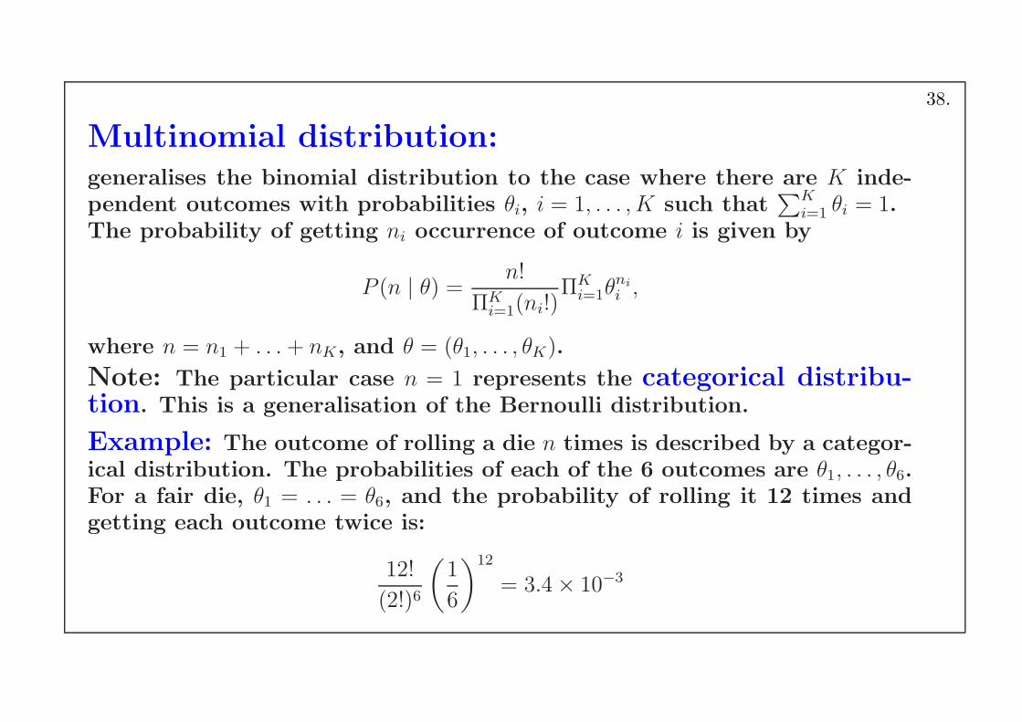
Multinomial distribution:generalises the binomial distribution to the case where there are K inde-pendent outcomes with probabilities θi, i = 1, . . . , K such that

∑Ki=1 θi = 1.

The probability of getting ni occurrence of outcome i is given by

P (n | θ) = n!

ΠKi=1(ni!)

ΠKi=1θ

ni

i ,

where n = n1 + . . .+ nK, and θ = (θ1, . . . , θK).

Note: The particular case n = 1 represents the categorical distribu-tion. This is a generalisation of the Bernoulli distribution.

Example: The outcome of rolling a die n times is described by a categor-ical distribution. The probabilities of each of the 6 outcomes are θ1, . . . , θ6.For a fair die, θ1 = . . . = θ6, and the probability of rolling it 12 times andgetting each outcome twice is:

12!

(2!)6

(

1

6

)12

= 3.4× 10−3

38.

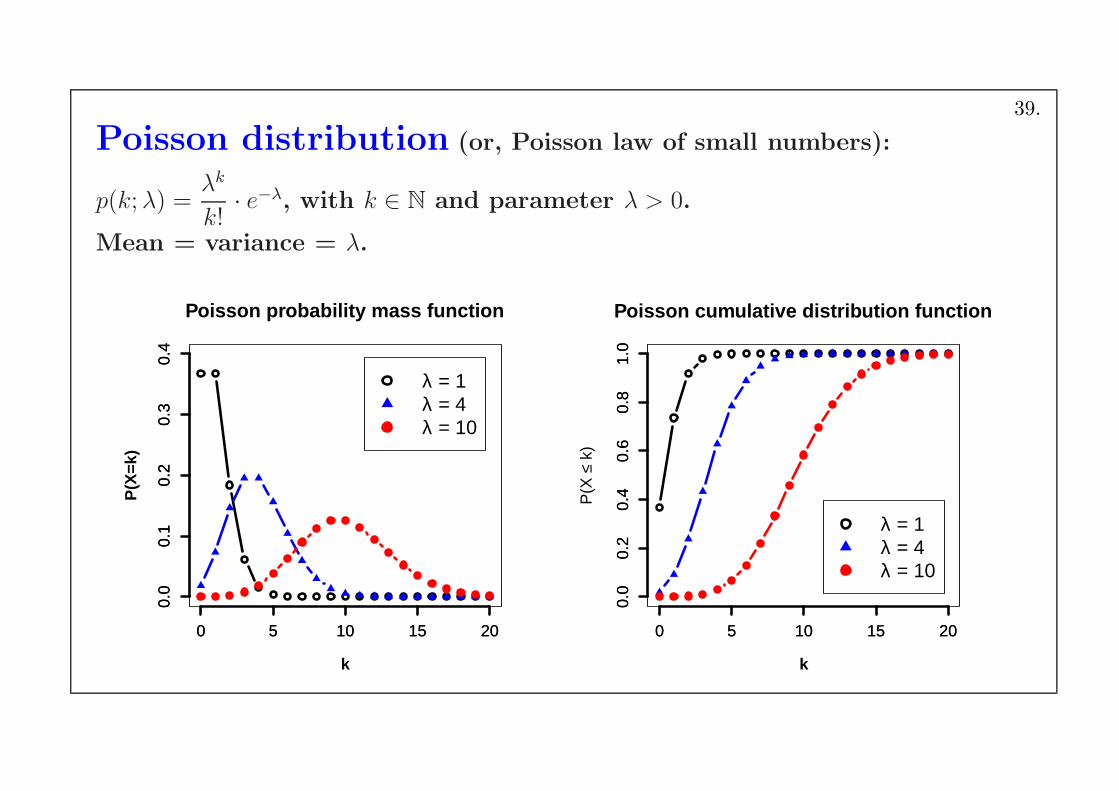
Poisson distribution (or, Poisson law of small numbers):

p(k;λ) =λk

k!· e−λ, with k ∈ N and parameter λ > 0.

Mean = variance = λ.

0 5 10 15 20

0.0

0.1

0.2

0.3

0.4

k

P(X

=k)

0 5 10 15 20

0.0

0.1

0.2

0.3

0.4

Poisson probability mass function

λ = 1λ = 4λ = 10

0 5 10 15 200.

00.

20.

40.

60.

81.

0

k

P(X

≤ k

)

0 5 10 15 200.

00.

20.

40.

60.

81.

0

Poisson cumulative distribution function

λ = 1λ = 4λ = 10

39.

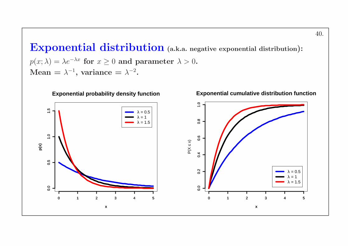
Exponential distribution (a.k.a. negative exponential distribution):

p(x;λ) = λe−λx for x ≥ 0 and parameter λ > 0.

Mean = λ−1, variance = λ−2.

0 1 2 3 4 5

0.0

0.5

1.0

1.5

x

p(x

)

0 1 2 3 4 5

0.0

0.5

1.0

1.5

Exponential probability density function

λ = 0.5λ = 1λ = 1.5

0 1 2 3 4 50.

00.

20.

40.

60.

81.

0

x

P(X

≤ x

)

0 1 2 3 4 50.

00.

20.

40.

60.

81.

0

Exponential cumulative distribution function

λ = 0.5λ = 1λ = 1.5

40.

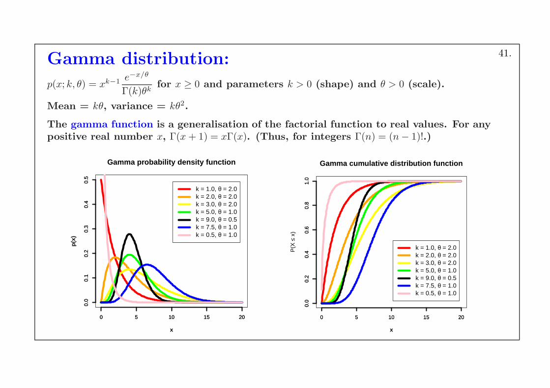
Gamma distribution:

p(x; k, θ) = xk−1 e−x/θ

Γ(k)θkfor x ≥ 0 and parameters k > 0 (shape) and θ > 0 (scale).

Mean = kθ, variance = kθ2.

The gamma function is a generalisation of the factorial function to real values. For anypositive real number x, Γ(x + 1) = xΓ(x). (Thus, for integers Γ(n) = (n− 1)!.)

0 5 10 15 20

0.0

0.1

0.2

0.3

0.4

0.5

x

p(x

)

0 5 10 15 20

0.0

0.1

0.2

0.3

0.4

0.5

Gamma probability density function

k = 1.0, θ = 2.0k = 2.0, θ = 2.0k = 3.0, θ = 2.0k = 5.0, θ = 1.0k = 9.0, θ = 0.5k = 7.5, θ = 1.0k = 0.5, θ = 1.0

0 5 10 15 20

0.0

0.2

0.4

0.6

0.8

1.0

x

P(X

≤ x

)

0 5 10 15 20

0.0

0.2

0.4

0.6

0.8

1.0

Gamma cumulative distribution function

k = 1.0, θ = 2.0k = 2.0, θ = 2.0k = 3.0, θ = 2.0k = 5.0, θ = 1.0k = 9.0, θ = 0.5k = 7.5, θ = 1.0k = 0.5, θ = 1.0

41.

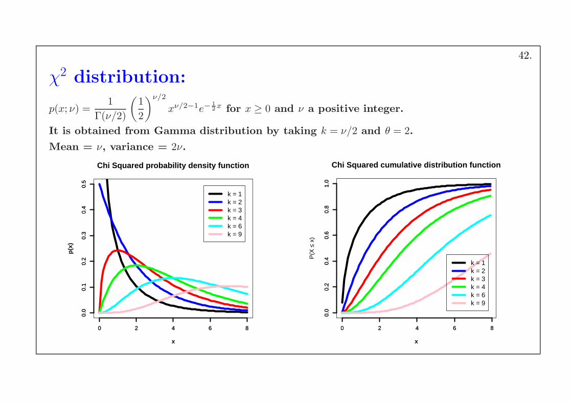
χ2 distribution:

p(x; ν) =1

Γ(ν/2)

(

1

2

)ν/2

xν/2−1e−1

2x for x ≥ 0 and ν a positive integer.

It is obtained from Gamma distribution by taking k = ν/2 and θ = 2.

Mean = ν, variance = 2ν.

0 2 4 6 8

0.0

0.1

0.2

0.3

0.4

0.5

x

p(x

)

0 2 4 6 8

0.0

0.1

0.2

0.3

0.4

0.5

Chi Squared probability density function

k = 1k = 2k = 3k = 4k = 6k = 9

0 2 4 6 80.

00.

20.

40.

60.

81.

0

x

P(X

≤ x

)

0 2 4 6 80.

00.

20.

40.

60.

81.

0

Chi Squared cumulative distribution function

k = 1k = 2k = 3k = 4k = 6k = 9

42.

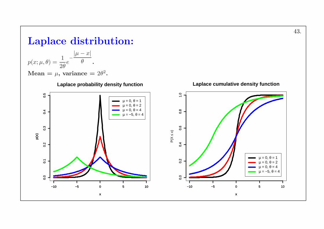
Laplace distribution:

p(x;µ, θ) =1

2θe−

|µ− x|θ .

Mean = µ, variance = 2θ2.

−10 −5 0 5 10

0.0

0.1

0.2

0.3

0.4

0.5

x

p(x

)

−10 −5 0 5 10

0.0

0.1

0.2

0.3

0.4

0.5

Laplace probability density function

µ = 0, θ = 1µ = 0, θ = 2µ = 0, θ = 4µ = −5, θ = 4

−10 −5 0 5 10

0.0

0.2

0.4

0.6

0.8

1.0

x

P(X

≤ x

)

−10 −5 0 5 10

0.0

0.2

0.4

0.6

0.8

1.0

Laplace cumulative density function

µ = 0, θ = 1µ = 0, θ = 2µ = 0, θ = 4µ = −5, θ = 4

43.

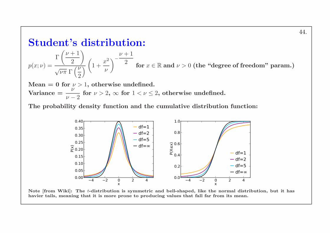
Student’s distribution:

p(x; ν) =

Γ

(

ν + 1

2

)

√νπ Γ

(ν

2

)

(

1 +x2

ν

)

−

ν + 1

2for x ∈ R and ν > 0 (the “degree of freedom” param.)

Mean = 0 for ν > 1, otherwise undefined.

Variance =ν

ν − 2for ν > 2, ∞ for 1 < ν ≤ 2, otherwise undefined.

The probability density function and the cumulative distribution function:

Note [from Wiki]: The t-distribution is symmetric and bell-shaped, like the normal distribution, but it hashavier tails, meaning that it is more prone to producing values that fall far from its mean.

44.

Dirichlet distribution:

D(θ | α) = 1

Z(α)ΠK

i=1θαi−1i δ(

∑Ki=1 θi − 1)

where

α = α1, . . . , αK with αi > 0 are the parameters,

θi satisfy 0 ≤ θi ≤ 1 and sum to 1, this being indicated by the delta functionterm δ(

∑

i θi − 1), and

the normalising factor can be expressed in terms of the gamma function:

Z(α) =∫

ΠKi=1θ

αi−1i δ(

∑

i −1)dθ =ΠiΓ(αi)

Γ(∑

i αi)

Mean of θi:αi

∑

j αj.

For K = 2, the Dirichlet distribution reduces to the more widely knownbeta distribution, and the normalising constant is the beta function.

45.

Remark:Concerning the multinomial and Dirichlet distributions:

The algebraic expression for the parameters θi is similar in the two distri-butions.However, the multinomial is a distribution over its exponents ni, whereasthe Dirichlet is a distribution over the numbers θi that are exponentiated.

The two distributions are said to be conjugate distributions and theirclose formal relationship leads to a harmonious interplay in many estima-tion problems.

Similarly,the beta distribution is the conjugate of the Bernoulli distribution, andthe gamma distribution is the conjugate of the Poisson distribution.

46.