Basic price optimization - Technical University of Denmark · optimization problem for a single product in a ... •Different firms competing in the same market face ... basic price

Basic price optimization

Brian Kallehauge

42134 Advanced Topics in Operations Research

Fall 2009

Revenue Management Session 03

08/10/2009Revenue Management Session 032 DTU Management Engineering,

Technical University of Denmark

Outline

• The price-response function

• Price response with competition

• Incremental costs

• The basic price optimization problem



Introduction to price optimization

• The basic pricing and revenue optimization problem can be formulated as an optimization problem.

– The objective is to maximize contribution:total revenue minus total incremental cost from sales.

• The key elements of the optimization problem is:

– the price-response function and

– the incremental cost of sales.

• In this lecture we will formulate and solve the pricing and revenue optimization problem for a single product in a single market without supply constraints.

• Furthermore, we will discuss some important optimality conditions.



The price-response function

• A fundamental input to any price and revenue optimization (PRO) analysis is the price-response function (or curve) d(p).

• There is one price-response function associated with each combination of product, market-segment, and channel in the PRO cube.

The price-response function, d(p), specifies demand for the product of a single seller as a function of the price, d, offered by that seller.

• This constrasts with the concept of a market demand curve which specifies how an entire market will respond to changing prices.

• Different firms competing in the same market face different price-response functions.

– The price-response functions may differ due to many factors, such as the effectiveness of their marketing campaigns, perceived customer differences in quality, product differences, location, etc.



Price-response functions in a perfectly competitive market

• In a perfectly competitive market:

– The price-response faced byan individual seller is avertical line at the market price.

– For higher prices,the demand drops to 0.

– If he prices below the market price,his demand equals the entire market.

• For example a wheat farmer:

– If he charges more than the marketprice, he will sell nothing.

– If he charges below the market price,the demand will be effectively infinite. Price-response curve in a

perfectly competitive market.



Commodities in a perfectly competitive market

• Commodity producers, such as the wheat farmer, have no pricing decision – the price is set by the operation of the larger market.

• I.e., in a competitive market, each firm only has to worry about how much output it wants to produce. Whatever it produces can only be sold at one price: the going market price.

• Therefore, sellers of true commodities in a perfectly competitive market have no need for pricing and revenue optimization (PRO).

• However, true comodities are surprisingly rare!



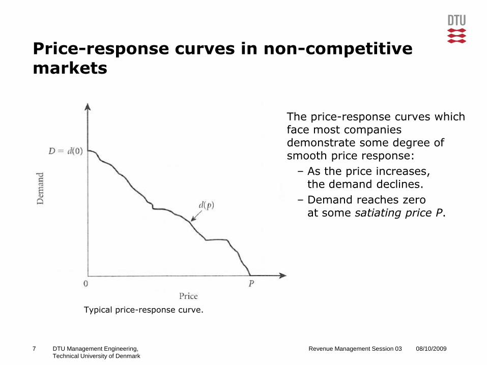
Price-response curves in non-competitive markets

Typical price-response curve.

The price-response curves whichface most companies demonstrate some degree of smooth price response:

– As the price increases,the demand declines.

– Demand reaches zeroat some satiating price P.



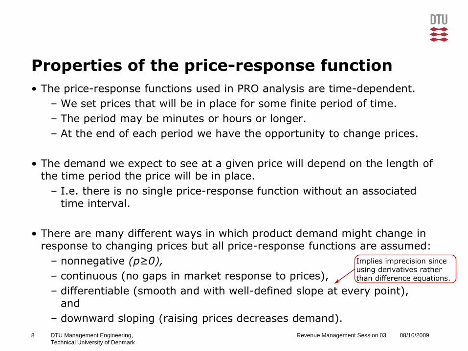
Properties of the price-response function

• The price-response functions used in PRO analysis are time-dependent.

– We set prices that will be in place for some finite period of time.

– The period may be minutes or hours or longer.

– At the end of each period we have the opportunity to change prices.

• The demand we expect to see at a given price will depend on the length of the time period the price will be in place.

– I.e. there is no single price-response function without an associated time interval.

• There are many different ways in which product demand might change in response to changing prices but all price-response functions are assumed:

– nonnegative (p≥0),

– continuous (no gaps in market response to prices),

– differentiable (smooth and with well-defined slope at every point),and

– downward sloping (raising prices decreases demand).

Implies imprecision since using derivatives rather than difference equations.



Measures of price sensitivity

• The two most common measures of price sensitivity are the slope and the elasticity of the price-response function.

– The slope measures how demand changes in response to a price change and equals the change in demand divided by the difference in prices.

– The price elasticity is defined as the ratio of the percentage change in demand to the percentage change in price.



The slope of price-response functions

• The slope equals the change in demand divided by the change in prices:

• Downward sloping: p1 > p2 implies d(p1) ≤ d(p2), i.e. δ(p1,p2) ≤ 0.

• The slope at a single price, p1, can be computed as the limit of the above equation as p2 approaches p1:

where d’(p1) is the derivative of the price-response function at p1.

• For small price changes we can write:

I.e. a large slope means that demand is more responsive to prices than a smaller slope.



The price elasticity of price-response functions

• The elasticity equals the percentage change in demand divided by the percentage change in prices:

where ε(p1,p2) is the elasticity of a price change from p1 to p2.

• This equation can be reduced to:

ε = 1.2 ε = 0.8

10 % price increase: 10 % price decrease:

12 % demand decrease. 8 % demand increase.

Since downwardsloping price-

response curve, ε(p1,p2) ≥ 0.

EX:



Point elasticity

• The price elasticity at a single price, p1, (”point elastiticy at p1”) can be computed as the limit of the above price elasticity equation as p2

approaches p1:

• I.e. the points elasticity is equal to –1 times the slope of the demand curve times the price divided by the demand.

• The point elasticity is useful as a local estimate of the change in demand resulting from a small change in price.

• Note that, unlike the slope, the price elasticity is independent of the units in which the price and demand is measured.



Price elasticity in practice

• The term price elasticity is often used as a synonym for price sensitivity.

– ”High price elasticity” items have very price sensitive demand, while ”low price elasticity” items have much less price sensitive demand.

• Often, a good with a price elasticity greater than 1 is described as elastic, while one with an elasticity less than 1 is described as inelastic.

• Elasticity is dependent on whether we measure the total market response if all suppliers of a product change their prices or the price-response elasticity for an individual supplier within the market.

– If all suppliers raise prices, the only alternative for customers is to purchase a substitute product or to go without.

– If a single supplier raises prices, customers can go to its competitor.

• Furthermore, as well as other aspects of price response, elasticity is dependent on the time period under consideration.

– There may be great difference in price elasticity in the short run and in the long run...



Price elasticity for different goods

• For most products, short-run elasticity is lower than long-run elasticitysince buyers have more flexibility to adjust to higher prices in the long run.

– For example, short-run elasticitiy for gasoline has been estimated to be 0.2, while the long-run elasticity has been estimated at 0.7.

– At first, consumers still need to by gasoline, but in the long term, people will change habits, e.g. buying higher mile-per-gallon cars.

• On the other hand, for many durable goods, such as cars and washing machines, the long-run price elasticity is lower than the short-run elasticity.

– The reason is that customers initially respond to a price rise by postponing the purchase of a new item.

– However, they will still purchase at some time in the future, so the long-run effect of the price change is less than the short-run effect.



Examples of price elasticity

• Salt has a low price elasticity as a respond to market price changes (people will by salt even if prices go up) but for an individual seller, the price elasticity would be expected to be high due to competitiveness.

• Airline tickets have a large long-term price elasticity since passengers will change their tavel habits if prices stay high.

• Cars have a low long-tirm elasticity since initially posponed purchashes will be be realized later in time even though prices stay high.



Price response and willingness to pay

• In reality, the price-response function is not simply given. Demand is the result of each potential customer observing the prices and deciding whether or not to buy a specific product.

• The price-response function specifies how many more of those potential customers would buy if we lowered our price and how many current buyers would not buy if we raised our price.

– I.e., the price-response function is based on assumptions about customer behavior.

• The most important part of models of customer behavior is based on willingness to pay (w.t.p).

• The willingness-to-pay approach assumes that each potential customer has a maximum willingness to pay (also called a ”reservation price”) for a given product.

– A customer will purchase if and only if the price is less than his/her maximum w.t.p.



Willingness to pay

• The number of customers whose maximum willingness to pay (w.t.p.) is at least p is denoted d(p).

– I.e., d(p) is the number of customers who are willing to pay the price p or more for the product.

• Define the function w(x) as the w.t.p. distribution across the population. Then for any values 0 ≤ p1 < p2:

is the fraction of the population that has w.t.p. between p1 and p2.

• Note that 0 ≤ w(x) ≤ 1 for all nonnegative values of x.



The willingness to pay distribution

• Let D = d(0), i.e. the number of customers willing to pay zero or more –i.e. willing to buy the product at all, be the maximum demand achievable. Then we can derive d(p) from the w.t.p distribution:

• Note that the price-response function is partitioned into two separate components: the total demand D and the w.t.p. distribution w(x).

• Next lecture considers examples of price-response functions and the basic price optimization problem.

Recall that d(p) is the number of customers who are willing to pay

the price p.

Simplified airline fare structures and marginal revenue transformation

Brian Kallehauge

42134 Advanced Topics in Operations Research

Fall 2009

Revenue Management Session 03



The low cost carrier competition led to simplified fare structures in scheduled airlines

Past Transition Future

Strong market segmentation Weakening of market

segmentation

• Intense LCC competition

• Price transparency

• Monopoly

Increasing market convergence

FirstBusiness

Economy

Business

Economy

• Consolidation of industry

First Business Economy

• Less-restricted fares

• Lower prices

• Traditional fare restrictions (AP, RT,

SA/SU, min/max)

• High fare ratios

• Stabilization of prices

Industry

Fare

structure

…simplified fares “is the most important pricing development in the

industry in the past 25 years” Tretheway (2004)



Without modifications of traditional RM systems fare simplification leads to spiral-down in revenues of 20-30%

Decrease in sales of high-

priced products

Decrease in

forecastDecrease in

protection

levels

Spiral-down

in revenues

20-30%

Fare

simplification

The root cause of

spiral-down is the

break-down of the

independent-demand

assumption of RM

systems



The fare simplification groups fares with similar restrictions into fare families

Fare families

Family 1

Family 2

Strong fence

1

2

3

4

5

6

Fence

Fare

simplification

Price-points

Strong fence

1

2

3

4

5

6

1-6

How do we

optimize the

revenue of the

fare families?

Fare classes

Independent demand model Lowest-open-fare demand model



The fare family network revenue

management problem with

dependent demand

The single-leg revenue

management problem with

independent demand

…vs. what we can solve

What we need to solve…

Marginal revenue transformation from

original fare structure to independent-

demand model

Decomposition approximation

1

2

Can Existing RM Systems be Saved?*

• Marginal revenue transformation (Fiig et al. 2009)

– The authors present a marginal revenue transformation that transforms

any fare structure (with any set of restrictions) into an independent demand

model.

– This allows all the traditional RM methods (that was invented assuming

independent demand) to be used unchanged.

– The standard availability control methods can be used unchanged provided

that the efficient frontier is nested (or approximately nested).

• Previous work has discussed methods to avoid spiral down and optimize

simplified fares.

– Sell-up models in Leg based EMSR, Belobaba and Weatherford (1996)

– Hybrid Forecasting of Price vs. Product Demand, Boyd, Kallesen (2005)

– DAVN-MR (Network optimization, mix of fully un-restricted and fully

restricted), Fiig et al (2005), Isler et al (2005).

– Fare Adjustment Methods with Hybrid forecasting, PROS, PODS research.

– Revenue Management with customer choice models, Talluri and van Ryzin

(2004), Gallego et al. (2007).

24

*Source: Thomas Fiig, Chief Scientist, Scandinavian Airlines.

OverviewFully differentiated

fare structure

Independent demand

by class

Class based RM-

system

25

OverviewFully un-differentiat

fare structure

Marginal Revenue

Transformation

Dependent demand

26

Fully differentiated

fare structure

Independent demand

by class

Class based RM-

system

OverviewFully un-differentiat

fare structure

Marginal Revenue

Transformation

Dependent demand

Any fare structure

Marginal Revenue

Transformation

Dependent demand

Independent

demand in policy

space

Map policies to

classes

Nested

policies

Yes

Policy based RM

No

27


fare structure

Independent demand

by class

Class based RM-

system


fi di Qi TRi MRi

$1.200 31,2 31,2 $37.486 $1.200

$1.000 10,9 42,2 $48.415 $1.000

$800 14,8 56,9 $60.217 $800

$600 19,9 76,8 $72.165 $600

$400 26,9 103,7 $82.918 $400

$200 36,3 140,0 $90.175 $200

28

Optimization: Fully differentiated- Deterministic Demand

- Single Leg

0

200

400

600

800

1000

1200

1400

0 50 100 150

Fare

Q

CAP

0

20000

40000

60000

80000

100000

0 50 100 150

TR

Q

k

j

jk dQ1

k

j

jjk dfTR1

29

Marginal Revenue (Intuitive derivation) -Fully un-differentiated,

- Single Leg

2f

2d

Revenue

recieved

Loss due to

buy-downNet revenue

2d

=

k

j

jk dQ1

kkk QfTR

Fully un-differentiated

fi di Qi TRi MRi

$1.200 31,2 31,2 $37.486 $1.200

$1.000 10,9 42,2 $42.167 $428

$800 14,8 56,9 $45.536 $228

$600 19,9 76,8 $46.100 $28

$400 26,9 103,7 $41.486 -$172

$200 36,3 140,0 $28.000 -$372

428$

2.312,42

486,37$167,42$

12

122

QQ

TRTRMR

10.9 *

$1000=

$10,900

31.2*

($1000-$1200)=

- $6,240

$10,900

-$6,240 =

$4,660

428$9.10

660,4$2MR2MR

30

Optimization: Fully un-differentiated- Deterministic Demand

- Single Leg

Fully un-differentiated

fi di Qi TRi MRi

$1.200 31,2 31,2 $37.486 $1.200

$1.000 10,9 42,2 $42.167 $428

$800 14,8 56,9 $45.536 $228

$600 19,9 76,8 $46.100 $28

$400 26,9 103,7 $41.486 -$172

$200 36,3 140,0 $28.000 -$372

-600

-400

-200

0

200

400

600

800

1000

1200

1400

0 50 100 150

Fare

Q

CAP

P(Q)

MR(Q)

0

20000

40000

60000

80000

100000

0 50 100 150

TR

Q

CAPdif f .

un-dif f .

Max

k

j

jk dQ1

kkk QfTR

31

Definition of policies

31

.

Policies: the set of fare products S that the airline chooses to

have open.

n classes gives potentially 2n policies. Examples could be:

All classes closed {},

All classes in economy open {E,…,T},

Only classes E,H, and K open: {E,H,K}.

Fare families: {Y,S; E,M,H,Q}

Nested policies:

Examples

Nested in economy: {},{E},{E,M},...,{E,M,...,L}

Non-nested in economy: {},{E},{E,H},...,{E,M,...,L}

lkSS lk ,

C

D

J

I

R

Y

S

B

E

M

H

Q

W

U

K

L

T

G

X

N

E

M

H

Q

W

U

K

L

T

C

D

J

Y

S

B

TRi-1

32

Optimization: General Formulation - Arbitrary fare structure

- Deterministic Demand

- Single Leg

32

Fare products

Policy (any set of open

classes)

Demand

Accumulated

Dem.

Total Revenue

Objective

Zj

j ZdZQ )()(

Zj

jj fZdZTR )()(

Demand Q

Total

RevenueEfficient Frontier

S1

Si-1

Si

d’i

Marginal

revenue: f’i

Qi-1 Qi

TRi

All policies Z

S0

CAP

Sm

},...3,1{},1{{},NZ

)(max ZTR

capZQts )(..

.

Optimum

njf j ,...,1,

)(Zd j

33

Marginal Revenue Transformation

Independent demandPolicies on the convex hull

Policy Dem. TR

... ...

Partition Dem. Adj. Fare

... ...

1S

2S

mS

1Q

2Q

mQ

1TR

2TR

mTR

1

'

1 Qd

12

'

2 QQd

1

'

mmm QQd

1

'

1 ff'

212

'

2 dTRTRf

'

1

'

mmmm dTRTRf

Marginal Revenue Transformation Theorem

• The transformed policies are independent.

• Optimization using the original fare structure and the marginal revenue

transformed in policy space gives identical results.

34

Mapping nested policies to Classes

Many choice models have the desirable property that the policies are nested

on the efficient frontier.

For nested policies we can assign demand and adj. fares back to the original

classes and continue reusing class based RM-systems.

Demand Q

Efficient

Frontier

S1

Sk-1

Sk

d’k

Qi-1 Qi

S0

Sm

Total

RevenueMapping from policies to classes

Newly added classes

Partitioned

demand

Split demand

any way between

newly added classes

Adj fare Assign the adjusted

fare to all newly

added classes.

1\ kk SS'

kd

Marginal

revenue: f’k

'

kf

35

Applications: Fully differentiated

demand

Assume fare class independence.

(the fare products are adequately differentiated, such that demand for a

particular fare product will only purchase that fare product)

Acc. demand Total Revenue

Partitioned demand Adjusted fare

Thus demand and fares are unchanged by the MR transformation.

Denote the unadjusted fare:

k

kj

j

kj

j

kkk

ddd

QQd

1,...,1,...,1

1

'

k

k

j

kj

jj

kj

j

kk

kk

k

fd

fdfd

QQ

TRTRf

1,...,1,...,1

1

1'

prod

kf'

kj

jk dQ,...,1 kj

jjk dfTR,...,1

36

Applications: Fully un-differentiated

demand

Passengers will only buy the lowest available fare

(demand for all other fare products except the lowest becomes zero)


Partitioned

demand

Adjusted

fare

price

kf'

knk psupQQ kkk fQTR

1

1

'

kkn

kkk

psuppsupQ

QQd

1

11

1

11

1

1'

kk

kkkk

kk

kkkk

kk

kkk

psuppsup

psupfpsupf

QQ

QfQf

QQ

TRTRf

Denote the adjusted fare:price

kd 'Denote the partitioned

demand:

Passengers will only buy the lowest available fare


Partitioned

demand

Adjusted

fare

is called the fare modifier

37

Applications: Fully un-differentiated

demand (exponential sell-up, equal spaced fare grid)

kkk fQTR))(exp( nknk ffQQ

)exp()exp(

)exp(

1

'

kk

nnk

ff

fQd,'

Mkk fff

)exp(1

)exp(Mf

where

Mf

38

Applications: Hybrid demand

The fare class demands are decomposed into contributions from both

differentiated (product-oriented) and un-differentiated (price-oriented)

demand


Partitioned

demand

Adjusted

fare

The adjusted fare in the hybrid case equals a demand-weighted average of:

– the unadjusted fare for the product-oriented demand

– the adjusted fare for the price-oriented demand.

where

k

price

kj

kj

prod

jk fdfdTR,...,1

price

k

kj

prod

jk ddQ,...,1

price

k

prod

k

prod

k

kdd

dr

price

k

prod

k

kkk

dd

QQd 1

'

.')1('

1

1'

price

kk

prod

kk

kk

kk

k

frfr

QQ

TRTRf

39

Extension to Stochastic models- Derivation using DP

Fare products

Policy (any set of open classes)

Arrival rate

Prob. of booking

Accumulated Dem.

Total Revenue

Objective (Bellman

recursion formula)

Zj

j ZpZQ )()(

Zj

jj fZpZTR )()(

},...4,2,1{},4,2{},...,3,1{},1{{},NZ

njf j ,...,1,

)(Zp j

)()(1

)1()()(max)(1

xJZQ

xJZQZTRxJ

t

t

NZt

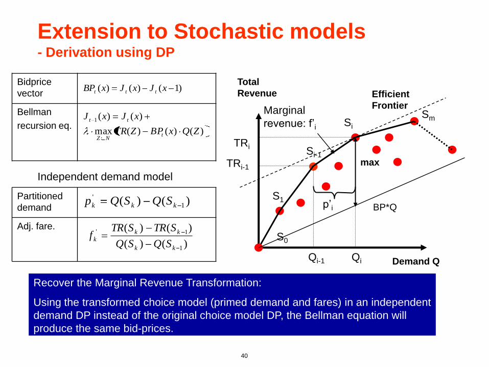
Bidprice

vector

Bellman

recursion eq.

40

Extension to Stochastic models- Derivation using DP

Demand Q

Total

Revenue Efficient

Frontier

S1

Si-1

Si

TRi-1

Qi-1 Qi

TRi

S0

Sm

max

BP*Qp’i

Marginal

revenue: f’i)()()(max

)()(1

ZQxBPZTR

xJxJ

tNZ

tt

)1()()( xJxJxBP ttt

Partitioned

demand

Adj. fare.

)()( 1

'

kkk SQSQp

)()(

)()(

1

1'

kk

kk

kSQSQ

STRSTRf

Recover the Marginal Revenue Transformation:

Using the transformed choice model (primed demand and fares) in an independent

demand DP instead of the original choice model DP, the Bellman equation will

produce the same bid-prices.

Independent demand model

41

Applications: EMSRb-MR

Fare Fare Mean Standard EMSRb Adjusted EMSRb-MR

Product Value Demand Deviation Limits Fares (MR) Limits

1 1,200$ 31.2 11.2 100 1,200$ 100

2 1,000$ 10.9 6.6 80 428$ 65

3 800$ 14.8 7.7 65 228$ 48

4 600$ 19.9 8.9 46 28$ 16

5 400$ 26.9 10.4 20 (172)$ 0

6 200$ 36.3 12.0 0 (372)$ 0

Cook book constructing EMSRb-MR (How to construct XXX-MR)

1. Determine the policies on the efficient frontier

2. Apply the marginal revenue transformation to both demands and fares.

3. Map policies back to classes

4. Apply EMSRb in the normal fashion using the transformed demands and fares.

Partitioned demand Adjusted fare Protection Level Booking Limit

),(~ 2'

kkk Nd'

kf'

,1

'

11

,1,1

' 1

k

kkkk

f

f''

kk capBL

EMSRb-MR applied to the un-restricted fare structure example.

42

Applications: DAVN-MR- Follow Cook Book

TOS

OSL

CPH

AMS

EWR

Differentiated

Undifferentiated

DAVN-MR constructed to handled a mix of fully differentiated

and undifferentiated fare structures.

Adj fare

Differentiated fare

products

The fare modifier since path are not

affected by risk of buy-down.

Un-differentiated

fare products

Mapped to lower buckets since

Thus fares are closed regardless of

remaining capacity. Thus avoiding spiral down.

• Assuming exponential sell-up and equally spaced

fares for simplicity.

• The fare modifier is calculated individually by path.

DCffDCffadj M'

0Mf

0Mf

Mff

43

H1(41)

19

28

H2(42)

4

3

2

1

10

9

8

7

6

5

15

1716

14

12

11 22

21

20

18

27

26

25

24

23

33

3231

30

29

39

38

37

36

3534

40

13

Traffic Flows

PODS Simulations

• PODS network D– 2 airlines. AL1and AL2

– 20 cities east/west. 2 hubs

– 126 legs in 3 banks

– 482 markets. 1446 paths.

• Sell-up parameters– Input Frat5 sell-up.

• Forecasting– Standard path/fare class forecasting

– Hybrid path/fare class forecasting

• Fare structure– 6 fare classes

– Unrestricted & Semi-restricted

• RM methods– Standard DAVN (std. forecast, no fare adj.) (Baseline)

– Hybrid DAVN (hybrid forecast. No fare adj.)

– Full DAVN-MR (hybrid forecasting and fare adj.)

• Competitive Scenarios– Monopoly and Competition

44

PODS Simulations- Fare structure

NONONO06

NONONO05

NONONO04

NONONO03

NONONO02

NONONO01

Non

Refund

Cancel

Fee

Min

Stay

APFARE

CLASS

SEMI-DIFFERENTIATEDUNDIFFERENTIATED

YESYESNO06

YESYESNO05

YESYESNO04

YESYESNO03

NOYESNO02

NONONO01

Non

Refund

Cancel

Fee

Min

Stay

APFARE

CLASS

• A un-differentiated structure

• A semi-differentiated structure

45

PODS Simulations-Monopoly Un-differentiated

100,0

115,8134,5

0

25

50

75

100

125

150

Standard Hybrid DAVN-MR

Re

ve

nu

e In

de

x

Monopoly: Un-differentiated fare-structure

85,4 85,1

74,1

0

20

40

60

80

100


Lo

ad

Fa

cto

r

Monopoly: Un-differentiated fare-structure

45

• Hybrid forecasting leads to 16% gain compared to standard due to reduced spiral down.

• Full DAVN-MR (hybrid forecasting + fare adjustment) adds an additional 18% gain.

• The effect comes from closing lower inefficient classes, which leads to lower LF.

46

PODS Simulations-Monopoly Semi-differentiated

46

108,7117,5

135,9

0

25

50

75

100

125

150


Re

ve

nu

e In

de

x

Monopoly: Semi-differentiated fare-structure

85,3 85,1

72,3

0

20

40

60

80

100


Lo

ad

Fa

cto

r

Monopoly: Semi-differentiated fare-structure

• Same overall trend compared to un-differentiated. Slightly less effect due to restrictions.

47

PODS Simulations-Competition Un-differentiated

47

100,0110,0

120,3

100,0 102,0

114,0

0

25

50

75

100

125

150


Re

ve

nu

e In

de

x

Competition: Un-differentiated fare-structure

AL1 AL2

85,5 84,8

68,5

84,4 85,593,1

0

25

50

75

100


Lo

ad

Fa

cto

r

Competition: Un-differentiated fare-structure

AL1 AL2

• Hybrid forecasting leads to 10% gain compared to standard. Less than monopoly due to

competition.

• Full DAVN-MR (hybrid forecasting + fare adjustment) adds an additional 10% gain.

• The effect comes from closing lower inefficient classes, which leads to lower LF.

48

PODS Simulations-Competition Semi-differentiated

99,7

112,9

128,9

99,7 101,9112,9

0

25

50

75

100

125

150


Re

ve

nu

e In

de

x

Competition: Semi-differentiated fare-structure

AL1 AL2

85,5 84,6

64,6

84,4 85,7

93,8

0

25

50

75

100


Lo

ad

Fa

cto

r

Competition: Semi-differentiated fare-structure

AL1 AL2

49

Conclusion

• Marginal revenue transformation transforms a general discrete choice model to an

equivalent independent demand model.

• The marginal revenue transformation allows traditional RM systems (that assumed

demand independence) to be used continuously.

• The marginal transformation is valid for:

– Static optimization

– Dynamic optimization

– Network optimization (provided the network problem is separable into

independent path choice probability).

• If the efficient frontier is nested (or approximately nested), the policies can be

remapped back to the original classes allowing the class based control mechanism

to be used in the standard way.

• DAVN-MR was tested using PODS for both un-differentiated and semi-

differentiated networks. Revenue gains are significant, 10-20 pct point better that

hybrid forecasting.

Documents

Basic price optimization - Technical University of Denmark · optimization problem for a single product in a ... •Different firms competing in the same market face ... basic price