Embed Size (px)
Citation preview


Basic Hypergeometric Functions and q-Calculus
Author
Dr. Farooq Ahmad Sheikh P.G., B.Ed, M.Phil, Ph.D. (Mathematics)
Recipient of Young Scientist Award from M.P. Council of Science and Technology – India (2013)
Assistant Professor (Mathematics) Department of Computer Science and Engineering,
Islamic University of Science and Technology – Awantipora – Kashmir
And
Co-Author
Dr. D. K. Jain M.Sc., M.Phil, Ph.D., NET(JFR) (Mathematics)
Department of Applied Mathematics Madhav Institute of Technology and Science, Gwalior (M.P.)
Published by
Corona Publication
Approved by : Gwalior, Jiwaji University, 2015
PhD. Thesis
Any brand names and product names mentioned in this book are subject to
trademark, brand or patent protection and are trademarks or registered trademarks of
their respective holders. The use of brand names, product names, common names,
trade names, product descriptions etc. even without a particular marking in this work
is in no way to be construed to mean that such names may be regarded as
unrestricted in respect of trademark and brand protection legislation and could thus
be used by anyone.
Publisher : Corona Publication, India
Website : http://www.coronapublication.com
E-mail: [email protected]
Printed in INDIA
Copyright @2014 by the author and Corona Publication, India and licensors
All rights reserved.

Preface
This book on Special Functions and Fractional Calculus has been specially written to
meet the requirements of the P.G. students and research scholar of all Indian
universities. The subject matter has been discussed in such a simple way that the
students will find no difficulty to understand it. The proofs of various theorems and
examples have been given with minute details. Each chapter of this book contains
complete theory and a fairly large number of solved examples.
During the preparation of the manuscript of this book, the author has incorporated the
fruitful academic suggestions provided by. Prof Renu Jain , Head SOMAAS, Jiwaji
University Gwalior (M.P.), Dr. D .K. Jain, Asst. Prof. Dept. of Applied
Mathematics Madhav Institute of Technology and Science, Gwalior (M.P.). Dr. M.
A. Khandy Asst. Professor in the Department of Mathematics at University of
Kashmir and Mr. Ehsan Ul Haq Sr.Lecture Zology J&k Education Department and
Mr. Sajad Saleem teacher J & k Education Department. It is expected to have a good
popularity due to its usefulness among its readers and users.
Words fail me in expressing my gratitude to my Respected brother Mr. A B.
Qayoom Sheikh & my beloved Wife for their consistent assistance and encouragement
through the years, which really helped me a lot. I find myself bereft of words when it
comes the turn of paying my deep sense of veneration to my parents and other
relatives. I express my deep sense of gratitude to my respected Teachers and dear
students of NCC and Pinacle Coaching centers for their consistent assistance and
encouragement through the years.
Last but not least; the authors are also very much thankful to the entire staff of
………corona publication Staff in particular Dr. B S Rathore ……. for taking keen
interest in publishing the book in its present shape.
Although, the authors have tried their best in the formulation of the subject matter
very nicely but that can be further improved based on the suggestions received from its
readers. Therefore, the constrictive and academic suggestions received from all sides
will always be welcomed and highly appreciated by the authors.

CHAPTER 1: GENERAL INTRODUCTION 1-33
1.1 Introduction 1.2 Introduction to Hypergeometric Functions
1.3 Some important Generalized Hypergeometric Functions 1.4 Basic Hypergeometric Series (q-series) 1.5 Fractional Calculus and its Elements 1.6 q- Fractional Calculus and its Elements 1.7 Conclusion CHAPTER 2: CERTAIN RESULTS OF BASIC ANALOGUE OF I-FUNCTION BASED ON FRACTIONAL q-INTEGRAL OPERATORS 34-44
2.1 Certain results of Basic Analogue of I-function based on Fractional q-integral Operators
2.2 Fractional Integral Operator of Riemann-Liouville type 2.3 Fractional Integral Operator of Kober type 2.4 Fractional Integral Operator of Saigo’s type 2.5 Special Cases 2.6 Conclusion
CHAPTER 3: DOUBLE INTEGRAL REPRESENTATION AND CERTAIN TRANSFORMATIONS FOR BASIC APPELL FUNCTIONS 45-60
3.1Double Integral representation and Certain Transformations for Basic Appell Functions 3.2 Integral representation for Basic Appell’s Hypergeometric Functions 3.3 Transformation Formulae for the q-Appell functions
3.4 Special Cases 3.5 Conclusion CHAPTER 4: RELATIONSHIP BETWEEN q-WEYL OPERATOR AND BASIC ANALOGUE OF I-FUNCTION WITH SPECIAL REFERENCE TO q-LAPLACE TRANSFORM. 61-67
4.1 Relationship between q-Weyl Operator and Basic Analogue of I-function with special reference to q- Laplace transform.
4.2q-Laplace Transform of Basic Analogue of I-function
4.3 Special Cases 4.4 Conclusion CHAPTER 5: CERTAIN QUANTUM CALCULUS OPERATORS ASSOCIATED WITH THE BASIC ANALOGUE OF FOX-WRIGHT HYPERGEOMETRIC FUNCTION 68-74
5.1 Certain Quantum Calculus Operators associated with the Basic Analogue of Fox-Wright Hypergeometric Function 5.2 Riemann- Liouville Fractional Integral Operators with the Basic Analogue of Fox-Wright Hypergeometric Function 5.3 Riemann- Liouville Fractional Derivative Operators with the Basic Analogue of Fox-Wright Hypergeometric Function 5.4 Conclusion
CHAPTER 6: SOME IDENTITIES OF THE GENERALIZED FUNCTION OF FRACTIONAL
CALCULUS INVOLVING GENERALIZED FRACTIONAL OPERATORS AND THEIR q-EXTENSION 75-89
6.1 Some Identities of the Generalized Function of Fractional Calculus Involving Generalized Fractional Operator 6.2.1 Left-sided Generalized Fractional Integration of the Generalized Function of Fractional Calculus 6.2.2 Right -sided Operator Generalized Fractional Integration of the Generalized Function of Fractional Calculus 6.3 Basic Analogue of R-function and Some of Its Identities

6.4Special Cases 6.5 Conclusion
CHAPTER 7: DIRICHLET AVERAGES OF GENERALIZED FOX-WRIGHT FUNCTION AND THEIR q-EXTENSION 90-102
7.1 Dirichlet Averages of Generalized Fox-Wright Function 7.2 Representation of 𝐑𝐤 and 𝐩𝐌𝐪 in terms of Reimann-Liouville Fractional Integrals
7.3 Representation of 𝐑𝐤 and 𝐩𝐌𝐪 in terms of q- Reimann-Liouville Fractional Integrals
7.4Special Cases 7.5 Conclusion
CHAPTER 8: REPRESENTATIONS OF DIRICHLET AVERAGES OF GENERALIZED R-FUNCTION
WITH CLASSICAL AND QUANTUM FRACTIONAL INTEGRALS 103-111
8.1 Generalized Functions for the Fractional Calculus and Dirichlet Averages 8.2 Representation of 𝐑𝐤 and 𝑴𝒒,𝒗 in terms of Reimann-Liouville Fractional Integrals
8.3 Representation of 𝐑𝐤 and 𝑴𝒒,𝒗 in terms of Quantum Fractional Integrals
8.4 Special Cases 8.5 Conclusion

1
1.1 Introduction
Our translation of real world problems to mathematical expressions relies on
calculus, which in turn relies on the differentiation and integration operations of
arbitrary order with a sort of misnomer fractional calculus which is also a
natural generalization of calculus and its mathematical history is equally long. It
plays a significant role in number of fields such as physics, rheology,
quantitative biology, electro-chemistry, scattering theory, diffusion, transport
theory, probability, elasticity, control theory, engineering mathematics and
many others. Fractional calculus like many other mathematical disciplines and
ideas has its origin in the quest of researchers for to expand its applicationsto
new fields. This freedom of order opens new dimensions and many problems of
applied sciences can be tackled in more efficient way by means of fractional
calculus.
The purpose of this thesis is to increase the accessibility of different dimensions
of q-fractional calculus and generalization of basic hypergeometric functions to
the real world problems of engineering, science and economics. Present chapter
reveals a brief history, definition and applications of basic hypergeometric
functions and their generalizations in light of different mathematical disciplines
2
of calculus, like fractional calculus, q- fractional calculus and Dirichlets
averages etc.
1.2 Introduction to Hypergeometric Functions
The study of one-variable hypergeometric functions is more than 200 years old.
They appear in the works of Euler, Gauss, Riemann, and Kummer. Their
integral representations were studied by Barnes and Mellin, and then special
properties of them by Schwarz and Goursat.The famous Gauss hypergeometric
equation is ubiquitous in mathematical physics as many well-known partial
differential equations may be reduced to Gauss‟s equation via separation of
variables. There are three possible ways in which one can characterize
hypergeometric functions: as functions represented by series whose coefficients
satisfy certain recursion properties; as solutions to a system of differential
equations which is, in an appropriate sense, holonomic and has mild
singularities and finally as functions defined by integrals such as the Mellin-
Barnes integral. For one-variable hypergeometric functions this interplay has
been well understood for several decades. In the several variables case, on the
other hand, it is possible to extend each one of these approaches but one may
get slightly different results. Thus, there is no universally accepted definition of
a multivariate hypergeometric function. For example, there is a notion due to
horn of multivariate hypergeometric series in terms of the coefficients of the
series. The recursions they satisfy gives rise to a system of partial differential

3
equations. It turns out that for more than two variables this system need not be
holonomic, i.e. the space of local solutions may be infinite dimensional. On the
other hand, there is a natural way to enlarge this system of PDE‟s into a
holonomic system. The relation between these two systems is well understood
only in the two variable cases [25]. Even in the case of the classical Horn,
Appell, Pochhammer, and Lauricella , multivariate hypergeometric functions it
is only in 1970‟s and 80‟s that an attempt was made by W. Miller Jr. and his
collaborators to study the Lie algebra of differential equations satisfied by these
functions and their relationship with the differential equations arising in
mathematical physics.
There has been a great revival of interest in the study of hypergeometric
functions in the last two decades. Indeed, a search for the title word
hypergeometric in the Math Sci Net database yields 3181 articles of which 1530
have been published after 1990! This newfound interest comes from the
connections between hypergeometric functions and many areas of mathematics
such as representation theory, algebraic geometry and Hodge theory,
combinatorics, D-modules, number theory, mirror symmetry, theory of
fractional calculus, theory of q-fractional calculus and now a day‟stheory of
quantum calculus (q-calculus)etc. An important new development in the theory
of hypergeometric functions by extending the number of parameters in the
Gauss function seems to have occurred for the first time in the work of Clausen

4
[2]. He introduced a series with three numerator parameters and two
denominator parameters. This idea was further extended to four to five
parameters and so on. Over the next hundred years, the well-known set of
special summation theorems associated with names of Salschutz [4], Dixon [5]
and Doughall [6] were developed. These are all for the series in which argument
is taken as unity. It can be shown that, Doughall„s theorem, the summation of
7F6 .series, is the most general possible theorem of this kind. The generalized
hyper geometric series pFq is defined as
(1.2.1)
Here no denominator parameter (j= 1, 2, 3,. . .q) is allowed to be zero or
negative integer. If any numerator parameter ( i = 1,2,3,. . . p) is zero or
negative integer, then the above series terminates. Moreover the series
converges if
(a) If p series converges for all finite z.
(b) If p = q+1, series converges for |z|<1 and diverges for |z|>1.
(c) If p > q+1, series diverges for z
1. 3 Some important generalized hypergeometric functions
Before looking at different dimensions of q-fractional calculus and
generalization of basic hypergeometric functions, we will first discuss some

5
useful generalized hypergeometric functionswhich are inherently related to the
work of the present thesis and will commonly be encountered. These include the
Meijer‟s G-Function, Fox's H-Function, I-Function, Appell‟s function, Fox-
Wright function, the Mittag-Leffler function, the more generalized function of
fractional calculus named as R-function. Also the basic analoguethese well-
known functions.
1.3.1 Meijer’s G-Function
The G-function was introduced by Cornels Simon Meijer (1936) as a very
general function intended to include most of the known special functions as
particular cases. This was not the only attempt of its kind. The generalized
hyper geometric function and MacrobertE-function had the same aim, but
Meijer‟s G-function was able to include these as particular case as well. The
majority of the special functions can be represented in terms of the G-functions.
The first definition was made by Meijer using a series, but now a day the
accepted and more general definition is in terms of Mellin-Barnes type integral.
Meijer‟s G-functions provides an interpretation of the symbol pFq when p>q+1.
The Meijer‟s G-function is defined as [10]

6
(1.3.1)
where an empty product is interpreted as 1. In above equation , 0< m < q,0< n<
p, and the parameters are such, that no pole of Γ(bj– s), j = 1, 2, 3, … , m
coincides with any pole of Γ(1- k+s), k = 1, 2,3,… ,n. There are three different
paths L of integration:
(i) L runs from -i∞ to +i∞ so that all the poles of Γ ( j-s), j = 1, 2, 3, …, m
are to the right side and all the poles of Γ (1- k+s), k= 1, 2, 3, … , n to
the left of L. The integral converges if (p+q) < 2 (m+n) and |argz|<[m+n
– – ]π
(ii) L is a loop starting and ending at +∞ and encircling all poles of bj-s),
j = 1, 2, 3… m, once in negative direction but none of the poles
of k=1,2,3… n. The integral converges if q>1 and either
p<q or p=q, and |z|<1,
(iii) L is a loop starting and ending at -∞and encircling all poles of Γ (1- k
+s),k = 1, 2, 3, …n once in the +ve direction but none of the poles of (bj-
s),j=1, 2, 3 … m.
It is always assumed that the values of parameters and of the variable are such
that at least one of the three definitions makes sense. In cases, when more than

7
one of these definitions makes sense, they lead the same result. Thus no
ambiguity arises. The integral converges if (p+q) < 2 (m+n) and |arg z|< (m+n -
) π, = 1, 2… r
1.3.2 Fox's H – Function
Although G-functions are quite general in character yet a number of special
functions, like Wright‟s generalized hypergeometric functions do not form their
special cases. Therefore Charles Fox introduced and studied a more general
function, known as Fox‟s H-function. This function contains all the
aforementioned functions, including G-function, as its special cases. Fox has
defined H-function in terms of a general Mellin-Barnes type integral. He also
investigated the most general Fourier kernel associated with the H- function and
obtained the asymptotic expansions of the kernel for large values of the
argument. Fox has also derived theorems about the H- function as asymmetric
Fourier kernel and established certain operational properties for this function.
The H – function is defined by Fox [12] as follows
(1.3.2)
Where

8
Here
(i) z ≠ 0 , z is a complex variable.
(ii) m, n, p and q non-negative integers satisfying 1<n<p and 1<m<q, and
for αj, j = 1, 2, 3, … p and for βj, j = 1, 2, … q.
(iii) The contour L runs from -i∞ to i∞ such that the poles of Γ( k- βk
s),
k = 1, 2, 3… m lies to the right of L and the poles ofΓ(1- + αj s), j =
1, 2, 3… n lies to the left of L.
1.3.3 I – Function
Fox‟s H-function was never a dead end of generalizations in the field of special
functions. The H-function was also generalized into a new type of function in
which the denominator parameters are in the summation form of Gamma
function products. This was named as the I-function.
TheI-function was introduced by Saxena [28] in connection with the solution of
a dual integral equations involving sum of H-functions as kernel. It is defined as
(1.3.3)
Where

9
pi(i= 1, 2, 3, … , r), qi (i= 1, 2, 3, … , r), m and n are integers satisfying
0< n < pi and 0< m < qi, r is finite and αj, βj, αji, βji, are complex numbers.
For I – function, there are three different paths L of integration
(i) L is a contour which runs from σ-i∞ to σ+i∞ (σ is real), so that all poles
of Γ( -βj s), j=1, 2, 3 … , m are to the right and all poles of Γ(1- +αjs),
j = 1, 2, 3… nare to the left of L.
(ii) L is a loop starting and ending at σ+i∞ and encircling all the poles
ofΓ( -βj s), j=1, 2, 3 … ,m. Once in the negative direction but none of
the pole of Γ(1- +αjs),j = 1, 2, 3, … , n. The integral converges if q > 1
and either pi< qiorpi=qi and |z|<|, I = 1, 2, 3, …, r
(iii) L is a loop starting and ending at σ+i∞ and encircling all the poles of Γ(1-
+αjs),once in positive direction, but none of the poles of Γ( -βj s), j =
1, 2, 3, … , m.
On specializing the parameters in I-function we can arrive at G and H functions.
Thus G and H functions are particular cases of I-function.

10
1.3.4 Appell’s Hypergeometric Functions of Two Variables
The hypergeometric series can also be generalized by simply increasing the
number of parameters.Some other generalizations have been studied by Appell
and Kampe De Feriet [8] in which the number of variables is increased.
If we consider the two hypergeometric series
F( , and F( )
And form their product,we obtain a double series, depending on the two
variables and y, in which the general term is
.
Next we replace one, two or three of the products ,
by the corresponding expressions( )m+n , ( )m+n ,
I)m+nrespectively.There are five possibilities, one of which gives the series
∑∑
This is simply the expansion of the function
The four remaining possibilities lead to the definition of Appellhypergeometric
functions of two variables, namely

11
(1.3.4.1)
(1.3.4.2)
(1.3.4.3)
(1.3.4.4)
The double series are absolutely convergent for
(i) | |<1, | |<1;
(ii) | |+|y|<1;
(1) | |<1, |y|<1;
(1) | |1/2
+ |y|1/2
<, respectively.
1.3.5 The Mittag-Leffler function
The Mittag-Leffler function arises naturally in the solution of fractional order
integral equations or fractional order differential equations, and especially in the
investigations of the fractional generalization of the kinetic equation, random
walks, Levy flights, super diffusive transport and in the study of complex
systems. The ordinary and generalized Mittag-Leffler functions interpolate
between a purely exponential law and power-law-like behavior of phenomena
governed by ordinary kinetic equations and their fractional counterparts. During
12
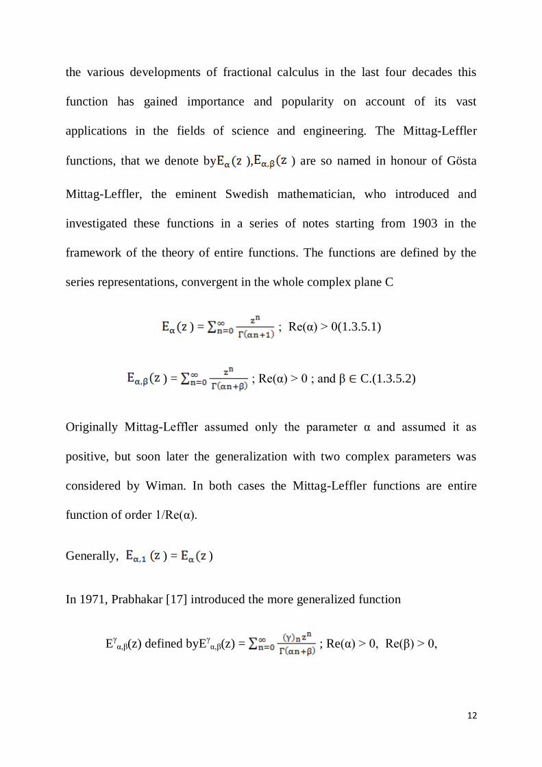
the various developments of fractional calculus in the last four decades this
function has gained importance and popularity on account of its vast
applications in the fields of science and engineering. The Mittag-Leffler
functions, that we denote by ), ) are so named in honour of Gösta
Mittag-Leffler, the eminent Swedish mathematician, who introduced and
investigated these functions in a series of notes starting from 1903 in the
framework of the theory of entire functions. The functions are defined by the
series representations, convergent in the whole complex plane C
) = ; Re(α) > 0(1.3.5.1)
) = ; Re(α) > 0 ; and β C.(1.3.5.2)
Originally Mittag-Leffler assumed only the parameter α and assumed it as
positive, but soon later the generalization with two complex parameters was
considered by Wiman. In both cases the Mittag-Leffler functions are entire
function of order 1/Re(α).
Generally, ) = )
In 1971, Prabhakar [17] introduced the more generalized function
Eγα,β(z) defined byE
γα,β(z) = ; Re(α) > 0, Re(β) > 0,

13
Re(γ) > 0; and α,β,γ C.
1.3.6Fox-Wright Generalized Hypergeometric Functions
Here we provide a survey of the higher transcendental functions related to the
Wright special functions. Like the functions of the Mittag-Leffler type, the
functions of the Wright type are known to play fundamental roles in various
applications of the fractional calculus. This is mainly due to the fact that they
are interrelated with the Mittag-Leffler functions through Laplace and Fourier
transformations.
We start providing the definitions in the complex plane for the general Wright
function and for two special cases that we call auxiliary functions. Then we
devote particular attention to the auxiliary functions in the real field, because
they admit a probabilistic interpretation related to the fundamental solutions of
certain evolution equations of fractional order. These equations are fundamental
to understand phenomena of anomalous diffusion or intermediate between
diffusion and wave propagation.
In mathematics, the Fox–Wright function (also known as Fox–Wright Psi
function or just Wright function) is a generalization of the generalized
hypergeometric function pFq(z) based on an idea of E. Maitland wright
(1935)[9]

14
pᴪq =
Where >0, (j = 1, . . . , p) and > 0 (j = 1, . . . , q) ; 1+ – ,
for suitably bounded values of |z|. In particular, when
= 1, (j = 1, . . . , p) and =1 (j = 1, . . . , q)
Wehave the following obvious relationship
pFq =
= pᴪq
The Fox-Wright function is a special case of the Fox-H-function as follows
pᴪq =

15
1.3.7 Generalized Functions for the Fractional Calculus(R-function)
It is of significant usefulness to develop a generalized function which when
fractionally differ integrated (by any order) returns itself. Such a function would
greatly ease the analysis of fractional order differential equations. To end this
process the following was proposed by Hartley and Lorenzo, 1998 [22]. The R-
function is unique in that it contains all of the derivatives and integrals of the F-
function. The R-function has the Eigen property that is it returns itself on qth
order differ-integration.Special cases of the R-function also include the
exponential function, the sin, cosine, hyperbolic sine and hyperbolic cosine
functions. The value of the R-function is clearly demonstrated in the dynamic
thermocouple problem where it enables the analyst to directly inverse transform
the Laplace domain solution, to obtain the time domain solution, and is defined
as follows
[ , , t] = .1)
The more compact notation
[ , t-c] =
When c = 0, we get
[ , t-c] =

16
Put v = q-1, we get Mittag - Leffler function
[ , t] = = E ( )
Taking a = 1, v = q-β
[1, t] = ( ).
The Laplace transform of the R-function is
L{ Rq,υ } = L{ }
= L{ }
Taking c= 0, we get
L{ Rq,υ } = , Re )>0, Re(s)>0.
1.4Basic Hypergeometric Series (q-series)
A basic hyper geometric function is an extension of an ordinary hyper
geometric function, by addition of an extra parameter when q →1,the basic
hypergeometric function tends towards an ordinary hypergeometric function.
These functions range from a simple series, analogous to the ordinary
exponential series, through basic Bessel and Whittaker functions, to generalized
basic hypergeometric functions in one or more variables.

17
The study of basic hypergeometric series (also called q-hypergeometric series or
q-series) essentially started in 1748, when Euler considered the infinite product
(q; q)∞ = , in connection with number of partition of a
positive integer. The subject remained dominated for a long time. It was about a
hundred years later that the subject acquired an independent status. When Heine
[3] converted a simple observation that = , into a systematic
theory of 2Ф1, basic hypergeometric series parallel to the theory of Gauss hyper
geometric series, 2F1.
This important discovery received impetus when Jackson [7] embarked on a
lifelong program of developing the theory of basic hypergeometric series in a
systematic manner.
The process of q-generalization of the hypergeometric series started in the1846
by Heine when he introduced the series.
1+ + +…
Whereit is assumed that c≠ 0, -1, -2, …, this series converges absolutely for |z|
<1 , when |q| <1 and it tends to Gauss‟s series as q →1.
The series defined above is usually called Heine‟s series.

18
1.4.1 Basic or q-analogues of H-functions
The q – analogues of H-function is terms of the Mellin –Barne's type basic
contour integral is given by Saxena [21] as
(1.4.1.1)
where G (qα) =
and 0< m < B, 0 < n < A; αj and βj are all +ve integers, and , are complex
numbers, where L is contour of integration running from - i∞ to i∞ in such a
manner so that all poles of G ( ) lie to right of the path and G ( )
are to the left of the path.The integral converges if Re [slog (z) – log sin πs} < 0,
for large values of |s| on the contour L, that is if where |q|<1.
The above definition can be used to define the q-analogues of Meijer's G-
function as follows:

19
Where 0< m< q, 0< n< p, and Re (s log z – log Sin πs) < 0
1.4.2 Basic analogue ofI – function
Saxena et al (1995) introduced the following basic analogue ofI–function in
terms of the Mellin–Barnes type basic contour integral as
(1.4.2.1)
where αj, βj, αji, βji, are real and +ve and j, j, ji, ji are complex numbers
Where L is contour of integration running from - i∞ to i∞ in such a manner so
that all poles of G lie to right of the path and though
G are to left of the path.The integral converges if Re [slog (z) – log
sin πs} < 0, for large values of |s| on the contour L, that is if
where |q|<1.

20
Taking r = 1, Ai = A, Bi = B, we get q – analogue ofH - function
1.4.3 Basic Analogue of Appell’s Hypergeometric
The basic analogue of Appell‟s hypergeometric functions of two variables were
defined and studied by Jackson [7]. Agarwal [16] also studied these functions
and gave some general identities involving these functions. Andrews [18] also
worked upon these functions and showed that the first of the Appell series can
be reduced to a 3Ф2 series.
Bhaskarand Shrivastava also defined bibasic Appell series and obtained
summation formulae, integral representation and continued fractions for these
functions Yadav and Purohit [27] employed the q-fractional calculus approach
to derive a number of summation formulae for the generalized basic
hypergeometric functions of one and more variables in terms of the q-gamma
functions.
Apart from Jackson‟s initial work, Agarwal developed some properties of basic
Appell series and Slater [14] applied contour integral techniques to such series
and observed that there was apparently no systematic attempt to find summation
theorems for basic Appell series.

21
Definition of basic analogue of Appell functions: These functions are defined as
1 (1.4.3.1)
2 (1.4.3.2)
3 (1.4.3.3)
4 (1.4.3.4)
where ( ;q)n =(1- )(1- q)(1- q2)…….(1- q
n-1)
and ( )∞
1.5 Fractional Calculus and its Elements
The concept of fractional calculus is not new. It is believed to have stemmed
from a question raised by L‟Hospital on September 30th
, 1695, in a letter to
Leibniz, about , Leibniz‟s notation for the nth derivative of the linear
function = .L‟Hospital curiously asked what the result would be if n= ?
Leibniz responded prophetically that it would be an apparent paradox from
which one day useful consequences would be drawn.

22
Following this unprecedented discussion, the subject of fractional calculus
caught the attention of other great mathematicians, many of whom directly or
indirectly contributed to its development. This included Euler, Laplace, Fourier,
Lacroix, Abel, Riemann and Liouville. Over the years, many mathematicians,
using their own notation and approach, have found various definitions that fit
the idea of a non-integer order integral or derivative. One version that has been
popularized in the world of fractional calculus is the Riemann-Liouville
definition. It is interesting to note that the Riemann-Liouville definition of a
fractional derivative gives the same result as that obtained by Lacroix [1].
Definition and properties of Fractional Integral Operators and Derivatives:
In this section we present a brief sketch of various operators of fractional
integration and fractional differentiation of arbitrary order. Among the various
operators studied, it involves the Riemann-Liouville fractional operators, weyl
operators and Saigo‟s operators etc. There are more than one version of the
fractional integral operator exist. The fractional integral can be defined as
follows
f( ) = ; ( >0), >0 (1.5.1)
It is called the Riemann version, where f( ) denote the fractional integration
of a function to an arbitrary order any nonnegative real number. In this
notation, and are the limits of integration operator. The other version of the

23
fractional integral is called the Liouville version. The case where negative
infinity in place of (1.5.2), namely,
f( ) = ; ( >0), >0. (1.5.2)
Thus, in general the Riemann-Liouville fractional integrals of arbitrary
order for a function f(t), is a natural consequence of the well-knownformula
(Cauchy-Dirichlets?) that reduces the calculation of the - fold primitive of a
function f ( ) to a single integral of convolution type
f( ) = ; ( >0) (1.5.3)
It is evident that the above integral is meaningful for any number provided its
real part is greater than zero. Further
f( ) = ; ( >0) , (1.5.4)
Is known as Riemann-Liouville right-sided fractional integral of order > 0
and
f( ) = ; ( >0) , (1.5.5)
is known as Riemann-Liouville left-sided fractional integral of order
> 0
24
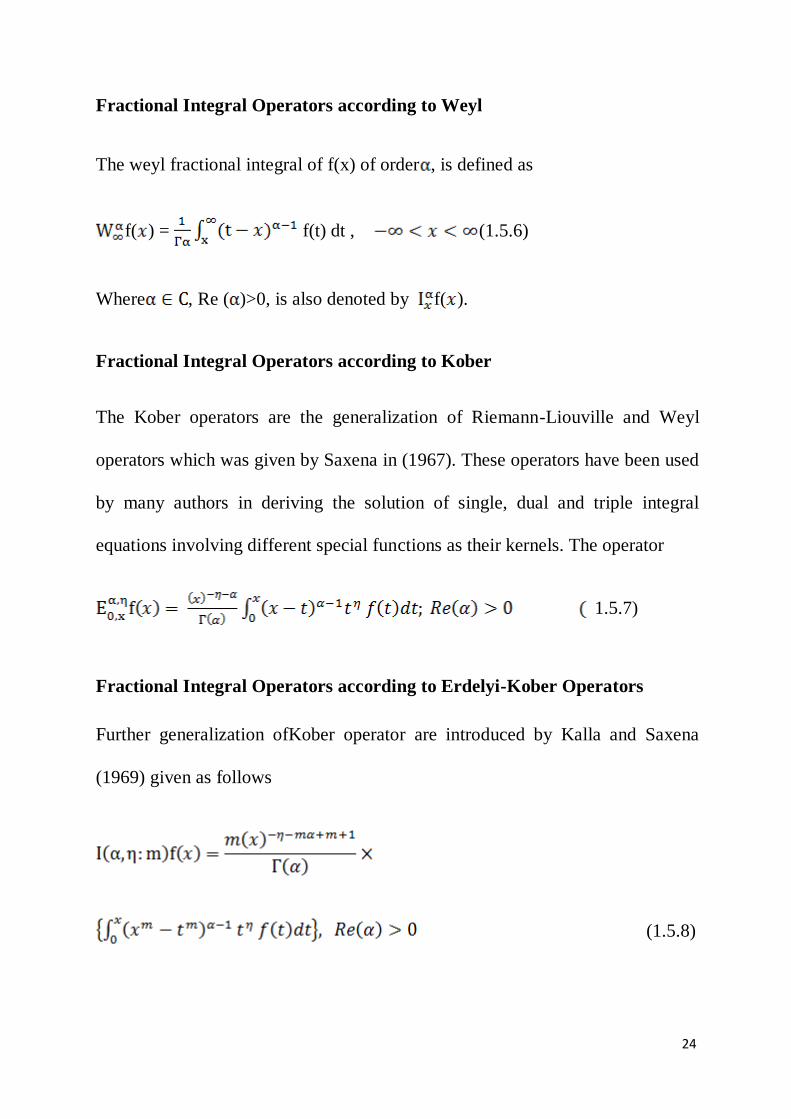
Fractional Integral Operators according to Weyl
The weyl fractional integral of f(x) of order , is defined as
f( ) = f(t) dt , (1.5.6)
Where , Re ( )>0, is also denoted by f( ).
Fractional Integral Operators according to Kober
The Kober operators are the generalization of Riemann-Liouville and Weyl
operators which was given by Saxena in (1967). These operators have been used
by many authors in deriving the solution of single, dual and triple integral
equations involving different special functions as their kernels. The operator
1.5.7)
Fractional Integral Operators according to Erdelyi-Kober Operators
Further generalization ofKober operator are introduced by Kalla and Saxena
(1969) given as follows
(1.5.8)

25
Fractional operators according to Saigo
Useful and interesting generalization of both the Riemann-Liouville and Erdlyi-
Kober fractional integration operators is introduced by Saigo [20], in terms of
Gauss‟s hypergeometric function as given below
Let and are complex numbers and let ( R+ the fractional
Re( )>0 and the fractional derivative Re( )<0 of the first kind of a function
= 2F1 f(t) dt,Re( )>0
= , 0<Re ( ) +η 1 (n N0) (1.5.9)
Fractional Derivative according to Riemann-Liouville
The notation that is used to denote the fractional derivative is f( ) for any
arbitrary number of order α.Fractional derivative can be defined in terms of the
fractional integral as follows
f(t) = [ f(t)]
Where0< u < 1, and n is the smallest integer greater than α such that u = n-α.
f(t) = f(t)
f(t) = (1.5.10)

26
Fractional Derivative Operators according to Weyl
The Weyl fractional derivative of order , denoted by , is defined by
f( ) =
f( ) = , (1.5.11)
Where , , m=0,1,2,3, ….
1.6 q- Fractional Calculus and its Elements
During the second half of the twentieth century, considerable amount of
research in fractional calculus was published in engineering literature. Indeed,
recent advances of fractional calculus are dominated by modern examples of
applications in differential and integral equations, physics, signal processing,
fluid mechanics, viscoelasticity, mathematical biology, and electrochemistry.
There is no doubt that fractional calculus has become an exciting new
mathematical method of solution of diverse problems in mathematics, science,
and engineering. Inspired by the great success of fractional calculus many
research workers, mathematician engaged their focus on another dimension of
calculus which sometimes called calculus without limits or popularly q-

27
calculus. The q-calculus was initiated in twenties of the last century. Kac and
Cheung‟s book [24] entitled “Quantum Calculus” provides the basics of such
type of calculus. The fractional q-calculus is the q-extension of the ordinary
fractional calculus. The present thesis deals with the investigations of q-
integrals and q-derivatives of arbitrary order, and has gained importance due to
its various applications in the areas like ordinary fractional calculus, solutions of
the q-difference (differential) and q-integral equations, q-transform analysis etc.
1.6 .1 Riemann-Liouville q-fractional operator
Agarwal [16], introduced the q-analogue of the Reimann-Liouville fractional
integral operator as follows.
f( ) = f(t) dq(t) (1.6.1.1)
Where α is an arbitrary order of integration such that Re (α)>0.
Jackson [7], Al.Salam [13] and Agarwal [16] defined basic integration as
= (1-q) f( )
From above two equations, we get
f ( ) = f( ) ( 1.6.1.2)

28
1.6.2 Kober Fractional q- Integral Operator
A basic analogue of the Kober fractional integral operator, as defined by
Agarwal [20] is given as
f( ) = (1.6.2.1)
Where 𝛍 is an arbitrary order of integration such that Re(𝛍) > 0 and 𝜂 being real
or complex.
Jackson [7], Al. Salam [13] and Agarwal [16] defined basic integration as
= (1-q) f( )
From above two equations, we get
f( ) = f( ) (1.6.2.2)
1.6.3 Weyl Fractional q- integral Operator
A basic analogue of Weyl fractional integral operator [13] is defined as
f( ) =
(1.6.3 .1)
1.6.4 Saigo’s q- Integral Operator
A basic analogue ofSaigo‟sfractional integral operator [29] is defined as

29
=
f(t) .
(1.6.4.1)
And
=
f (t ) .
By making use q- integral definition, the above operators can be written as
=
f( )
And =
f(
) (1.6.4.2)

30
1.7 Conclusion
This chapter is of introductory in nature. Here we throws light on the origin and
historical developments of special functions like Gauss hypergeometric
functions and its Mellin–Barnes integral representation including E- function ,
Meijer‟s G-function, Fox‟s H- function, Saxena‟sI-function, Mittag-Leffler
function and generalized functions for the fractional calculus (R-
function).Generalized hypergeometric functions, basic hypergeometric series
(q-series), fractional calculus and its elements have been discussed extensively
in the different chapters of the present work. Moreoverthis chapter also gives
details of q- fractional calculus and its elements such as q- Reimann-Liouville
fractional integral and differential operator, q-weyl operators and q-Saigo‟s
operators etc. have been also discussed extensively in various chapters of this
thesis. The purpose of studying theories is to apply them to real world problems.
Over the last few years, mathematicians pulled the subject of q-fractional
calculus to several applied fields of engineering, science and economics etc. The
authors believe that the volume of research in the area of q- fractional calculus
will continue to grow in the forth coming years and that it will constitute an
important tool in the scientific progress of mankind.

31
References
[1]. Lacroix, S (1819), Traite du Calcul Differentiel et du Calcul Intégral, 2nd
edition, pp. 409-
410.
[2]. Clausen, T. (1828), Uber Die Falle Wenn Die Reihe Y= 1+ +…, J. Fur. Maths, 3, 89-
95.
[3]. Heine, E (1847), Untersuchunger under die Riehe 1+
+ +… J. math; 34, 285-328.
[4]. Saal Schutz, L (1890), Eine summations formel zeitschr Fur maths and Physik.
[5]. Dixon, A(1903), Summation of certain series, Proc. London Math Soc. (1), 35, 285-298.
[6]. Dougall, J. (1907), on vander mode‟s theorem and some more general expansions, Proc.
Edin. Math.Soc. 217-234.
[7]. Jackson, F. H (1910), On basic double Hypergeometric function, Quart, J. Pure and Appl.
Math; 41, 193-203.
[8]. Appell, P. and Kampe de Feriet, J.(1926), Functions Hypergeometriqueset Hyperspheriques
Polynomes d'Hermite . Gauthier-Viliars, Paris.
[9]. Wright, E.M (1935), The asymptotic expansion of generalized hypergeometric function. J.
London Math. So, 10, 286-293.
[10]. Meijer, C. S. (1936), On the G-Function, Proc. Nat. Acad. Watensh, 49, 227-237, 344-356,
457-469.
[11]. Baily, W. N (1961), Generalized hypergeometric series, Cambridge University, Press.
[12]. Fox, C (1965), The G and H-functions as symmetrical Fourier Kernels. Trans. Amer.
Math. Soc. 98, 395-429.
[13]. Al. Salam, W. A (1966), Some fractional q- integral and q- derivatives. Proc. Edin. Math.
Soc.17, 616-621.

32
[14]. Slater, L.J (1966), Generalized Hypergeometric function, Cambridge University, Press.
[15]. Saxena, R. K. (1967). On fractional integration operators. Math. Z. Vol. 96, pp. 288-291.
[16]. Agrawal, R. P (1969), Certain fraction q-integrals and q-derivatives. Proc. Edin. Math.
Soc., 66, 365-370.
[17]. Prabhakar, T.R (1971), A singular integral equation with a generalized Mittag-Leffler
function in the kernel, Yokohama Math. J. Vol.19, 7-15.
[18]. George E. Andrews. (1972), Basic Hypergeometric series, J. London Math. Soc. (2) 4 618.
[19]. Exton, H. (1978), Hand book of Hypergeometric integrals, Ellis Horwood Limited,
Publishers, Chechester.
[20]. Saigo, M. Saxena, R.K. (1992), and Ram, J. On the fractional calculus operator associated
with the H- function, Ganita Sandesh, 6(1), 36-47.
[21]. Saxena, R.K., Rajendra Kumar (1995), Abasic Analogue of the Generalized H-function Le
Mathematiche Vol.L- Fase II 263-271.
[22]. Hartley, T.T and Lorenzo, C.F (1998), A solution to the fundamental linear fractional
order differential equation, NASA\TP.
[23]. Eduardo Cattani (1999), Lecture notes on hypergeometric functions in Computer Science
1719 19- 28.
[24]. Kac,V. Chebing,P. (2002). Quantum Calculus, University, Springer –Verlog, NewYork.
[25]. Dickenstein,A, Matusevich, L. F. and Sadykov, T (2005), bivariate hypergeometric D-
modules. Adv. Math., 196(1):78–123,
[26]. Saxena, R. K, Yadav, R. K, Purohit, S. D and Kalla, S. L (2005), Kober fractional q-
integral operator of the basic analogue of the H-function,3-8.
[27]. Yadav, R.K., Purohit, S.D (2006), on fractions q-derivatives and transformation of the
generalized basic hypergeometric functions, Indian Acad. Math.2,321-326.
[28]. Saxena, V. P, (2008), The I-function, Anamaya Publishers Pvt. Ltd, New Delhi.

33
[29]. Yadav, R. K. Purohit, S. D (2010), On generalized fractional q-integral operators involving
the q-Gauss hypergeometric functions, Bulletin of Mathematical Analysis and
Applications. Vol(2),35-44.
[30]. Capelas de Oliveira. E, F. Mainardi and J. Vaz Jr (2011), Modelsbased on Mittag-Leffler
functions for anomalous relaxation in dielectrics European Journal of Physics, Special
Topics, Vol. 193.
[31]. Amera Almusharrf (2011), Development of fractional trigonometry and an applications of
fractional calculus to pharmacokinetic model , A Thesis Presented to the Faculty of the
Department of Mathematics and Computer Science Western Kentucky University Bowling
Green, Kentucky.

34
Certain results of basic analogue of i-function based on fractional q-
integral operators
In this chapter q-analogue of the Saxena‟s I-functions has been mentioned in
connection with q-fractional integral operators. This function is a significant
generalization of Fox‟s H- function which was introduced by Saxena [4] and
later on modified by Jain etal,byintroduced an alternative definition of the basic
analogue of a generalization of well-known Fox's H – function in terms of I-
function using q-Gamma functiondefined as follows[10]. More over a number
of useful results of basic analogue of I-function have been derived by making
use of different techniques of fractional q-integral operators including Reimann-
Liouville, Kober fractional and Saigo‟s fractional q- integral operators. Some
special cases have also discussed.
Definitions and preliminaries used in this chapter based on the text by Gasper
and Rehman [5] are given as follows
Basic analogue of I-function is
(2.1.1)
Where 0 < m < , 0 < n < ; i= 1,2,3,…r; r is finite. Also aj, bj , aij and bij , are
complex numbers and αi , βi, αij, βij are real and +ve integers. Where L is

35
contour of integration running from - i∞ to i∞ in such a manner so that all poles
of ); 1 to right of the path and those of
); 1 The integral converges if Re [s log
(x) – log sin πs} < 0, for large values of |s| on the contour L.
In the theory of q-calculus, 0 |q|< 1 .The q-shifted factorial is defined as
= (2.1.2)
Moreover,
= 1,
Or equivalently
=
Further if αis any complex number,then the definition can be stated as follows
=
= (2.1.3)
Theq-analogue of power function is defined and denoted as
= ( ;q)= = (2.1.4)
The q- gamma function is defined by
( = ( ; 𝛂 R(0,-1,-2,…)

36
Where =
The q-derivatives of a function f(x) is given by [5]
, ≠0)and 0=0(2.1.5)
as q ⤏1
We have
( ) = , R(µ) + 1 > 0
The q-integral of a function is defined as [5]
f( ), (2.1.6)
f( ), (2.1.7)
f( ), (2.1.8)
The q- binomial theorem is as follows
1φ0[α;q; ] (2.1.9)
The q- analogues of Gauss summation theorem [5] is given by
2φ1[ ]=
Agarwal [1] introduced the q-analogue of the Reimann-Liouville fractional
integral operator as follows.
( )= (2.1.11)

37
Where µ is an arbitrary order of integration such that Re (μ) From equation
(2.1.6) and (2.1.11), we get
( )= ( (2.1.12)
Agarwal [1], introduced the basic analogue of Kober fractional operator as
follows.
=
Again from equation (2.1.11) and (2.1.12), we get
( ) = ( (2.1.13)
The q- gamma function is defined by
( =( ; 𝛂 R(0,-1,-2,…)
Where = .
Recently, Purohit and Yadav [9] defined q-analogue of Saigo‟s fractional
integral operator as follows
( ) =
(2.1.14)
( ) = (2.1.15)
Now from equations (2.1.13) and (2.1.14)

38
( ) = (
(2.1.16)
2.2 Fractional Integral Operator of Riemann-Liouville Type
In this section, we will evaluate the following fractional q-integral operator of
Riemann-Liouville involving basic analogue of I-function.
Theorem 2.2 .1
Proof: To prove theorem (2.2.1) when λ , we apply (2.1.12) and (2.1.1) to
the left side, and we get
s
On summing the inner 1φ0 series with help of (2.1.9) we get

39
Now using (2.1.3), we get
Also when λ 0 in theorem (2.2.1) we get a known result due to Yadav etal[7]
as follows
2.3 Fractional Integral Operator of Kober Type
In this section, we will evaluate the following fractional q-integral operator of
Kober type involving basic analogue of I-function.
Theorem(2.3.1) = (

40
Proof: To prove theorem (2.3.1) when λ , we apply (2.1.14) and (2.1.1) to
the left side, and we get
= (
This implies
= (
1φ0 [ ;q ; ]
On summing the iner1φ0 serieswith help of (2.1.9) we get
=(
Now using (2.1.1) we get
= (

41
Also when λ 0 in theorem (2.3.1) we get a known result due to Yadav etal[6]
as follows
= (
2.4 Fractional Integral Operator of Saigo’s Type
In this section, we will evaluate the following fractional q-integral operator of
Saigo‟s type involving basic analogue of I-function.
Theorem (2.4.1) For 0 Re (α) η being complex
=
Proof: To prove theorem (2.4.1) when λ , we apply (2.1.14) and (2.1.1) to the
left side, and we get

42
This implies
Now taking β = 0, α = η and λ in the above theorem (2.4.1) we get
2.5 Special Cases
In this section, we discuss some of the important special cases of the main
results established discussed above, If we take r =1 in the theorems (2.2.1) and
(2.3.1), we get well known results reported in [6,7] of the basic analogue of H-
function involving Riemann- Liouville and Kober fractional q-integral
operators, namely, when λ , then
=

43
(2.5.2)
2.6 Conclusion
The results proved in this chapter give some contributions to the theory of the
basic hypergeometric functions and are believed to be a new contribution to the
theory of q-fractional calculus and are likely to find certain applications to the
solution of the fractional q-integral equations involving various q-
hypergeometric functions. In this connection one can refer to the work of Yadav
and Purohit [6].
Reference
[1]. Agrawal. R.P (1966), Certain fractional q-integrals q-derivatives, Proc.Camb.Philos.Soc.66
(365-370).
[2]. SlaterL. J (1966), Generalized Hypergeometric Functions, Cambridge UniversityPress.
[3]. Exton. H (1978), q-Hypergeometric Functions and Applications, Ellis Horwood Limited,
Publishers, Chechester.
[4]. Saxena R.K, Modi G.C and Kalla S.L(1983), A basic analogue of Fox‟sH-function, Rev.
Technology Univ, Zulin, 6, pp. 139-143.
[5]. Gasper.G and Rahman.M (1990), Basic Hypergeometric series, CambridgeUniversityPress.
[6]. SaxenaR.K, YadavR.K, PurohitS.D (2005), and S.L Kalla, Kober fractional q-integral
operator of the basic analogue of the H-function, Rev. Technology Univ., Zulin, Vol.28,No.2.
pp. 154-158.

44
[7]. Kalla S.L, Yadav R.K and. PurohitS.D(2005), On the Riemann-Liouville fractional q-integral
operator of the basic analogue of Fox H-function, Fractional Calculus and Applied analysis.
Vol 8. Number 3.pp.313-322.
[8]. RajKovicP.M., MarinkovicS.D. andStankovicM.S(2007), Applicable Analysis and Discrete
Mathematics, Vol.1pp.1-13.
[9]. PurohitS.D. and YadavR.K(2010), On generalized fractional q-integral operator involving the
q-Gauss hypergeometric functions, Bull. Math.Anal.Appl. Vol.2, issue(4), pp.35-44.
[10]. Jain D. K, Jain. R and Farooq Ahmad (2012); Some Transformation Formula for Basic
Analogue of I-function; Asian Journal of Mathematics and Statistics, 5(4), 158-162.

45
Double integral representation and certain transformations for basic appell
functions
Apart from Jackson‟s initial work, Agarwal developed some properties of basic
Appell series and Slater [3] applied contour integral techniques to such series
and observed that there was apparently no systematic attempt to find summation
theorems for basic Appell series. Sharma and Jain [8] showed that q-Appell
functions can be brought within the preview of Lie-theory by deriving reduction
formulae for q-Appell functions namely using the dynamical
symmetry algebra of basic hypergeometric function 2Ф1.
The basic analogue of Appell‟s hypergeometric functions of two variables were
defined and studied by Jackson [1].Agarwal [4] also studied these functions and
gave some general identities involving these functions. Andrews [5] also
worked upon these functions and showed that the first of the Appell series can
be reduced to a 3Ф2 series.
Bhaskar and Shrivastava also defined bibasic Appell series and obtained
summation formulae, integral representation and continued fractions for these
functions Yadav and Purohit [7] employed the q-fractional calculus approach to
derive a number of summation formulae for the generalized basic

46
hypergeometric functions of one and more variables in terms of the q-gamma
functions.
In the present chapter we have studied basic analogue of Appell‟s
hypergeometric functions called q-Appell functions and express these
functions1 2
, 3
in terms of definite integrals. Also certain transformation
formulae have been obtained related these functions. Some special cases have
been also discussed.
3.1 Definitions and preliminaries used in this chapter based on the text by
Gasper and Rehman [5] are given as follows
We shall use the following usual basic hypergeometric notations for
|q| <1,
( ; q) n =(1- ) (1- q) (1- q2)… (1- q
n-1)
And (
, and ( ; q)0 = 1 (3.1.1)
1 (3.1.2)
2 (3.1.3)
3 (3.1.4)

47
4 (3.1.5)
3.2 Integral Representation for Basic Appell’s Hypergeometric Functions
In this section, by using the definition of q-integral, we express the basic
Appell functions 1
,2,
3in terms of double integrals which takes the
form of ordinary Appell’s hypergeometric functions as a limiting case.
Theorem (3.2.1):2
=
taken over the the triangle, The parameters are of
course, supposed to be such that the double integrals are convergent. The
formulae are readily proved by expanding the integrand in the powers of and
y and integrating term by term. There appears so such integral representation for
the 4 function.
Proof:
2 (3.2.1)
Since, =
Therefore,

48
=
= .
=
Now making use of q-beta function, we have
=
=
(3.2.2)
Using above result in (3 .2.1), we get
2=
Using series manipulation in (3.2.3), we get

49
2=
Thus, we get
2=
.
This completes the proof of the theorem.
Similarly we can easily prove the following theorems.
Theorem (3.2.2):
1
Taken over the triangle u , u + v
Proof:
Since u + v

50
Or v u
Therefore,
=
=
Put v = u) w
u)
Thus, we have
=
Or

51
Or
= )
Or
=
Or
= 1
Theorem (3.2.3):3
=
Proof:
=

52
=
Put v = u) w
u)
Thus, we have
=
Or
=
Finally, we get the result
3
=
Theorem (3.2.4):1

53
Proof:
1 =
Since,
=
= B ( )
From above equation, we have
1 =
Thus, we have the result as follows
1
3.3 Transformation formulae for the q-Appell functions
In this section we have derived certain transformation formulae for the q-Appell
functions.

54
Theorem (3.3.1):
1 3
Proof:
1
2ɸ1
Hence,
1 =
3
This completes the proof.
Theorem(3.3.2):
2 2

55
Proof:
2
=
=
= 2ɸ1
= 2ɸ1
Hence,
2=
2
This completes the proof of the theorem.
Similarly we can easily prove the following theorems.
Theorem (3.3.3):2( ; b, ) =
1
Proof:
2( ; b, )
=

56
Or
2( ; b, )
=
= ɸ
= ɸ
= ɸ
= ɸ
= ɸ
= ɸ
=
=
=
=

57
=
Since, =
=
Letting , we have
2( ; b, ) =
=
Thus, finally we have
2( ; b, ) =
1
Theorem (3.3.4):1
=
1
Proof: To prove (3.3.4) from L.H.S, we have
1 =

58
L.H.S =
L.H.S =
Therefore, we have
1 =
1 =
1 =
1
3.4 Special Cases
In this section, we discuss some of the special cases of the main results
established in the previous section two. As q→1, the above results take the form
of well-known transformation formulae of classical Appell functions F1 2
, F3
in terms of definite integrals. The formulae given by [2] are as follows
2=
(3.4.1)
1
= ×

59
). (3.4.2)
3 =
). (3.4.3)
3.5 Conclusion
In this chapter, we have explored the possibility for derivation of some integral
representation and transformation formulae for basic hypergeometric functions
of one and more variables in particular the q-Appell functions, using certain
fundamental tools of q-fractional calculus. The results thus derived are general
in character and likely to find certain applications in the theory of basic
hypergeometric functions. In this connection one can refer to the work of Baily
[2] and Sharma [8].
Reference
[1]. Jackson, F. H (1910), On basic double Hyper geometric function, Quart, J. Pure and Appl.
Math; 41, 193-203.
[2]. Baily. W.N (1935), Generalized hypergeomtric series, Cambridge Math. Cambridge Univ.
Press.
[3]. Slater, L.J. (1966), Generalized Hypergeometric function, Cambridge University, Press.
[4]. Agrawal, R. P (1969), certain fraction q-integrals and q-derivatives. Proc. Edin. Math. Soc., 66,
365-370.
[5]. George E. Andrews (1972); Basic hypergeometric series, J. LondonMath. Soc. (2) 4 (1972),
618.
[6]. Gasper .G and Rahman.M (1990), Basic hypergeometric series, Cambridge University Press.

60
[7]. Yadav R.K, Purohit S.D (2006), on fractions q-derivatives and transformationof the generalized
basic hypergeometric functions, Indian Acad. Math.2,321-326.
[8]. Sharma.K and Jain.R (2007), Lie-theory and q-Appell functions, Proceedings of the National
Academy of Science India, 77, 259-262.

61
Relationship between q-weyl operator and basic analogue of i-function with
special reference to q-laplace transform.
The fractional q- calculus is the q-extension of the ordinary fractional calculus.
The subject deals with the investigations of q-integrals and q- derivatives of
arbitrary order, and has gained importance due its various applications in the
areas like ordinary fractional calculus , solution of the q-differential and q-
integral equations , q-transform analysis [5,6and 8]. Motivated by these avenues
of applications, a numbers of workers have made use of these operators to
evaluate fractional q-calculus, basic analogue of H- function, basic analogue of
I-function, general class of q-polynomials etc.
The q-derivatives and q- integrals are part of so called quantum calculus [7]. In
this chapter, we investigate how such derivatives and integrals can be possibly
used in establishing a formula exhibiting relationship between basic analogue of
q-weyl operator and q-Laplace transform, which allows the straight forward
derivation ofsome useful results involving weyl operator and basic analogue of
I-functionin terms of q-gamma function [11]. Also some special cases have
been discussed.
Al-Salam[2, 4] introduced the q-analogue of weyl fractional integral operator in
the following manner.

62
= f (t ) ; Re (α) > 0 (4.1.1)
Also, Hahn [1] defined the q-analogues of the well-known classic Laplace transform
Φ(s) = . (4.1.2)
By means of the following q-integrals
{f (t)} = f(t) . (4.1.3)
{f (t)} = f (t) (4.1.4)
Where the q-exponential series is defined as
= (4.1.5)
(4.1.6)
R.Jain, etal [11] define the basic analogue of I-function in terms of q-gamma
function as follows
=
(4.1.7)
Where 0 < m < , 0 < n < ; i= 1,2,3,…r; r is finite. Also aj, bj , aij and bij , are
complex numbers and αi , βi, αij, βij are real and +ve integers. Where L is
contour of integration running from - i∞ to i∞ in such a manner so that all poles

63
of ); 1 to right of the path and those of
); 1 The integral converges if Re [s log
(x) – log sin πs} < 0, for large values of |s| on the contour L.
4.2 Main results
In this section, we will derive the q-Laplace transform of basic analogue ofI-
functionby making make use of equations (4.1.7) and (4.1.3).
Proposition:q-Laplace transform of basic analogue of I-function
{ }=
=
Where
= , we have
{ }= = (z; p). (4.2.1)
In this section, we establish a theorem with the help of above preposition
involving q-Laplace transform of basic analogue of I-function and q-weyl
operator.
64
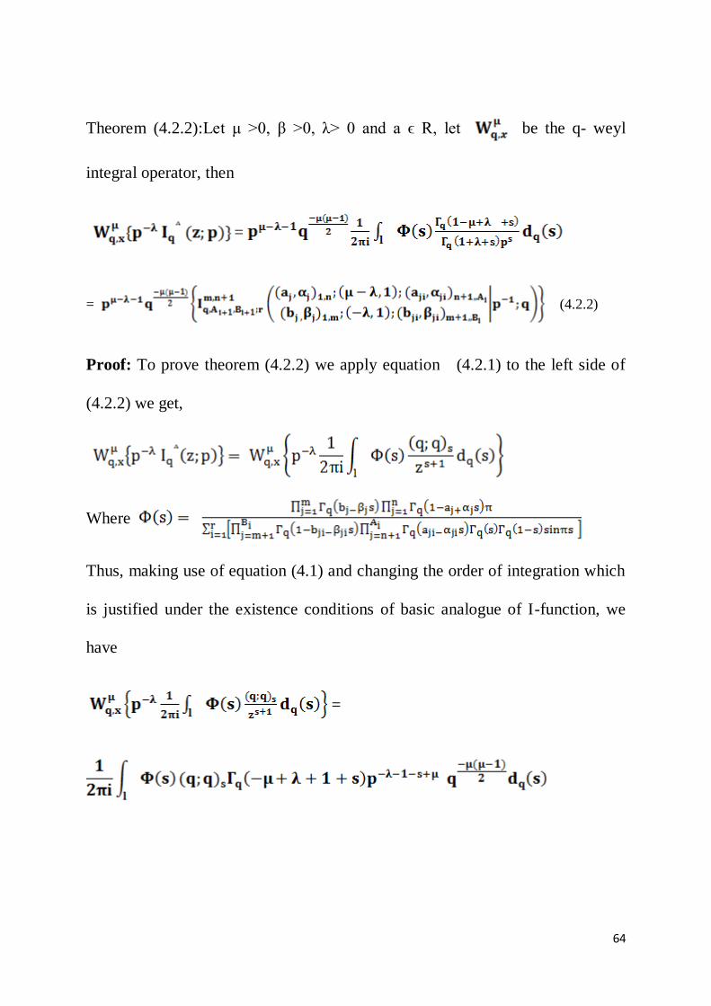
Theorem (4.2.2):Let μ >0, β >0, λ> 0 and a ϵ R, let be the q- weyl
integral operator, then
=
= (4.2.2)
Proof: To prove theorem (4.2.2) we apply equation (4.2.1) to the left side of
(4.2.2) we get,
Where
Thus, making use of equation (4.1) and changing the order of integration which
is justified under the existence conditions of basic analogue of I-function, we
have
=

65
Hence, we get =
(4.3)
4.3 Special cases
Corollary 1:By setting r = 1 and q = 1 in equation (4.1.7) and abovetheorem,
then it takes the form of Fox‟s H-function [3]
=
Andin this cases result becomes
=
= .
By setting q = 1 in the above preposition, we get well-known results
established by Singh [10]
{ } = = (z;p).
By setting q = 1 in the above preposition, we get well-known results
established by Singh [10]

66
=
= .
4.4 Conclusion
The results proved in this chapter gives the evaluation of the q-Laplace
transforms of basic analogues of the I-function functions in relation with the q-
weyl fractional operator. It has many applications in sciences and engineering
for its special fundamental properties. In this connection one can refer to the
work ofPurohit and Kalla [9], where they studied q-analogues of the Sumudu
transform and derived some fundamental properties. Alsoevaluated the q-
Sumudutransform of basic analogue of Fox‟s H-function.
Reference
[1]. Hahn. W (1949), Uber die höheren Heineschen Reihen und eine einheitliche Theorie
dersogenannten speziellen Functionen, Math Nachr, 2, 257-294. MR. 12, 711.
[2]. Al. Salam. W. A (1952-1953), q-analogues of Cauchy‟s formula, Proc. Am. Math. Soc17, 182-
184.
[3]. Fox. C. (1965), A formal solution of certain dual integral equations, Amer, Math; Soc.119.
[4]. Al. Salam W.A(1969), Some fractional q-integrals and q-derivatives, Proc. Edinb. Math.Soc, 15,
135-140.
[5]. Samko.G, Kilbas.A.Marichev (1993), Fractional integrals and Derivatives; theory and
applications, Gordon and Breach, Yverdon.
[6]. Podlubny.I (1999), Fractional Differential Equations, Academic Press.
[7]. Kac.V. and Cheung.P (2002), Quantum Calculus, University, Springer-Verlag, New York.

67
[8]. Kilbas.A, Srivastava .M.H and Trujillo.J.J (2006.), Theory and Applications offractional
differential, North Holland Mathematics studies 204.
[9]. Kalla S.L and Purohit S.D (2007), ON q-Laplace transform of the q- Bessel functions, Fractional
Calculus and Applied analysis. Vol 10. Number 3.pp.190-196.
[10]. Singh. Dinesh (2011), A study of fractional calculus operators with special reference to integro-
differential equations;A Ph.D. thesis, Jiwaji University, Gwalior.
[11]. Jain D. K, Jain.R and Farooq Ahmad (2012); Some Transformation Formula for Basic Analogue
of I-function; Asian Journal of Mathematics and Statistics, 5(4), 158-162.

68
Certain Quantum Calculus Operators Associated with the Basic Analogue
of Fox-Wright Hypergeometric Function
The objective of this chapter is to derive the relationship that exists between the
basic analogue of Fox-Wright hypergeometric function (z;q) and the
quantum calculus operators, in particular Riemann-Liouville q-integral and q-
differential operators. Some special cases have been also discussed.
Kac and Cheung‟s book [6] entitled “Quantum Calculus” provides for the basics
of so called q-calculus. More details on this type of calculus can also be found
in Andrews [5,2].
Let us consider the following expression
Now letting → , we get the well-known definition of the derivative of a
function at . However ever , if we take or + h
,where q is a fixed number different from 1, and h a fixed number different from
0, and don‟t take the limit , we enter the fascinating world of quantum calculus.
The corresponding expressions are the definitions of the q-derivative and h-
derivative of as defined in [6 & 3]. The same was latter on introduced by F.

69
H. Jackson in the beginning of the twentieth century. He was the first to develop
q- calculus in a systematic way.
The basic analogue of Fox-Wright hypergeometric function denoted P Q(z;q)
for z ϵ C is defined in series form as [6]
(z;q)= ,where |q|<1. (5.1.1)
Where ϵ C >0; ; 1+ ≥ 0; ϵR , for
suitably bounded value of |z|. Moreover in view of the relation
(z;q) = =
the function PᴪQ (z; q) converges under the convergence conditions of the well-
known Fox‟s H-function which are as follows, the
integralconverges , on the contour C, where
0<|q|< 1 verified by Saxena, et al [3] .
Agrawal [1] introduced the basic analogue of the Reimann-Liouville fractional
operator as follows.
= f(t) ; Re(α) > 0. (5.1.2)
In particular, for f(x) = , we have

70
= ; Re(α) > 0 (5.1.3)
Also q-analogue of the Reimann-Liouville fractional derivative defined as [1]
( ) ; Re (α) < 0, and |q|<1 (5.1.4)
In particular, for f(x) = , we have
= ; Re(α) < 0,|q|<1. (5.1.5)
Theorem (5.2): Let α >0,β>0,γ > 0 and a ϵ R, let be the Riemann-
Liouville fractional integral operator, then
=
Proof: To prove theorem (5.2) we apply equations (5.1.1) and (5.1.2) to the left
side of theorem (5.2) we get
)= )

71
) = )
Making the use of equation (5.1.3) we get
This completes proof of the theorem.
Corollary (5.2.1): For α >0, β> 0,γ,λ> 0 , then
( ) (5.2.1)
Corollary (5.2.2): By setting δ = 1 in equation (5.2.1)we get
( ) (5.2.2)

72
Theorem (5.3): Let Re (α) <0 , β> 0, γ > 0 and ϵ R, let be the Riemann-
Liouville fractional derivative operator, then there holds following results
=
Proof: To prove theorem (5.3) we apply equations (5.1.1) and (5.1.4) to the left
side of theorem (5.3) we get,
=
) )
Making the use of equation (5.1.5) we get
=
Corollary (5.3.1): For Re (α)<0,β> 0, and γ >0, then

73
( )(5.3.1)Corollary
(5.3.2):By setting δ = 1 in equation (5.3.1) we get
( ) (5.3.2)
By setting q = 1 in the equations (5.2.1),(5.2.2),(5.3.1) and (5.3.2) we get well-
known results established by Saxena and Saigo [2] and [10]
( ) (5.4.3)
By setting δ = 1 in equation (5.4.3) we get
( ) (5.4.4)
( )(5.4.5)By setting
δ = 1 in equation (5.4.5)we get
( ). (5.4.6)
5.4 Conclusion
Finally,in mathematics, specifically in the areas of combinatorics and special
functions, a q-analog of a theorem, identity or expression is a generalization
involving a new parameter q that returns the original theorem, identity or

74
expression in the limit as q → 1. Typically, mathematicians are interested in q-
analogues that arise naturally, rather than in arbitrarily contriving q-analogues
of known results.
Reference
[1]. Jackson, F. H (1910); On basic double Hyper geometric function, Quart, Math.
[2]. Andrews, G.E, (1986), q-seriestheir development and application in analysis, number theory,
combinatorics, physics and computer algebra. In CBMS Regional Conference Lecture. Series in
Mathematics, Vol. 66. Amer. Math. Soc, Providence.
[3]. Gasper.G; Rahman.M, (1990). Basic hypergeometric series and its application, Vol. 35
[4]. Saxena. R.K; Rajendra kumar, (1995). A Basic analogue of the Generalized H- function, Le
Mathematiche, pp. 263-271.
[5]. Andrews.G.E,Askey,R.Roy,R.(1999).Special Functions, Cambridge University Press.
[6]. Kac, V, Chebing, P (2002), Quantum Calculus, University, Springer –Verlog, New York.
[7]. Saxena. R.K; Saigo.M (2005); Certain properties of fractional operators associated with
generalized Mittag-Leffler function, Fractional calculus and Applied analysis. 8. pp. 141-154.
[8]. Srivastava. H.M (2007), Some Fox-Wright Generalized Hypergeometric Function and
Associated Families of Convolution Operators; Applicable Analysis and Discrete Mathematics,
Vol.1 pp.56-71.
[9]. Jain. R; Singh.D, (2011). Certain Fractional Calculus Operators associated with Fox-Wright
Generalized Hypergeometric function, Jnanabha, Vol.41, pp.1-8.
[10]. Jain. D.K; Jain.R;Farooq ahmad(2013), Some Remarks on Generalized q-Mittag-Leffler
Function in Relation with Quantum Calculus Published International Journal of Advanced
Research Volume 1, Issue 4, 463-467.

75
Some identities of the generalized function of fractional calculus involving
generalized fractional operators and their q-extension
This chapter is divided into two sections, in first section we made attempt to
establish some identities of the ordinary functions of classical fractional
calculus. In the second section we deal the basic analogue of the generalized
function of fractional calculus and its identities.
During last few decades, scientists and applied mathematicians, found the
fractional calculus to be immensely useful in diverse number of fields, such as
rheology, quantitative biology, electro- chemistry, scattering theory, diffusion,
transport theory, probability, elasticity, control theory and many others. The
properties of well-known fractional operators and their generalizations have
been used to solve various fractional differential and integral equations
representing these phenomena.
In this chapter, we study certain inherent properties of the family of the
generalized fractional operators, which were introduced and investigated in
several works by different researchers including Kalla, Saxena, Srivastava, et al.
The purpose of this paper is to study the generalized fractional integral
operators and in relationship with the generalized function of

76
fractional calculus (R-function introduced by Lorenzo and Hartley) which is an
entire function of the form,
= , where µ>0 .
A more compact notation is given as
= ,
which is particularly useful when c=0.
6.1 Definitions and preliminaries used in this chapter
The fractional calculus, like many other mathematical disciplines and ideas has
its origin in the quest of researchers for extension of meaning. It extends the
derivative of an integer order to an arbitrary order. This freedom of order opens
a new dimension and many problems of applied sciences can be tackled more
effectively by recourse to fractional calculus. Applications of fractional calculus
require fractional derivatives and integrals of different kinds [15, 12].
Differentiation and integration of fractional order are traditionally defined by
right and left sided Riemann-Liouville fractional integral operators and
and corresponding Riemann-Liouville fractional derivatives and ,
asfollows
= dt;( >0).

77
= dt;( >0).
And
( ) = , Re (α)≥ 0;
An interesting and useful generalization of the Riemann-Liouville and Erdlyi-
Kober fractional integral operators has been introduced by Saigo [1] in terms of
Gauss- hypergeometric function as follows.
,
.
Now we summarize various functions that have been found useful in several
boundary value problems of fractional calculus.
(i) Mittag-Leffler Function: The function (z) defined by the series
representation
(t) = , >0, t C.
Mittag-Leffler [3], Wiman [7] and Agarwal [2] investigated the generalization
of the above function (z) in the following manner [7].
(t) = , υ>0,ρ>0, t C.

78
Where C is the set of complex numbers.
A more generalized form of Mittag-Leffler function is introduced by Prabhaker
[3] as
(z) = .
The generalized Fox-Wright function pѱq(z) defined for z C, , C and
R ( is given by the series
pѱq(t) = pѱq =
(ii) Robotnov and Hartley’s function: To affect the direct solution of the
fundamental linear fractional order differential equation, the following was
introduced by Hartley and Lorenzo as below
= , >0.
(iii) Generalized function of fractional calculus:
This function was defined by Hartley and Lorenzo, 1998 [8] as a generalization
of all the above mentioned functions. This function has a remarkable and useful
property that it returns itself when differ- integrated fractionally.
υ = , >0.

79
The Laplace transform of the R-function is
L { } = L{ }
= L{ }
Taking c= 0, we get
L { } = , Re )>0, Re(s)>0.
Agrawal [1] introduced the basic analogue of the Reimann-Liouville fractional
operator as follows.
= f(t) ; Re(α) > 0.
In particular, for f(x) = , we have
= ; Re(α) > 0
Also q-analogue of the Reimann-Liouville fractional derivative defined as
( ) ; Re (α) < 0, and |q|<1
in particular, for f(x) = , we have
= ; Re(α) < 0,|q|<1.

80
6.2 Left-sided generalized fractional integration of the generalized function
of fractional calculus
In this section, we consider the left-sided generalized fractional integration of
the generalized function of fractional calculus and making use of the given
lemma to derive following useful results.
Lemma: Let α, β, γ >0, and ρ C.
(a) If Re (ρ) >max [0, Re (β-γ)], then as reported in [5] , we have
=
(b) If Re (ρ) >max [Re(-β), Re(-γ)],
) .
Theorem (6.2.1):Let α, β, γ, ρ δ C, be complex numbers such that Re(α) >0
, Re( )>0, υ>0 and and ) be the left-sided operator of the
generalized fractional integration associated with Gauss-hypergeometric
function . Then there holds the following relationship
=
3ѱ3
Provided each member of the equation exists.

81
Proof:By using the definition of the generalized function of fractional calculus
and the fractional integral operator, we get
=
By the use of Gaussian hypergeometric series [6] , series form of the
generalized function of fractional calculus, interchanging the order of
integration and summation and evaluating the inner integral , by the known
formula of Beta integral , and making use of above lemma , we get
=
)
=
=
=

82
3ѱ3
Interchanging the order of integration and summations, which is permissible
under the conditions, stated with the theorem due to convergence of the integral
involved in the process? This completes the proof of the theorem.
Corollary1: ForRe (α >0),Re ( )>0, υ>0 and putting c = 0 , = - ,
then there holds the formula
=
3ѱ3
Theorem (6.2.2) : Let α,β,γ, ρ δ C, be complex numbers such that Re(α) >0
, Re(α+ )> max[-Re(β),-Re(γ)] with υ>0 and and ) be the right -
sided operator of the generalized fractional integration associated with Gauss-
hypergeometric function . Then there holds the following relationship
3ѱ3

83
Provided each member of the equation exists.
Proof:By using the definition of the generalized function of fractional calculus
and the fractional integral operator, we get
=
)
By the use of Gaussians hypergeometric series [6] , series form of the
generalized function of fractional calculus , interchanging the order of
integration and summation and evaluating the inner integral , by the known
formula of beta integral , and making use of above lemma , we get
=
=
=
3ѱ3

84
6.3 Basic Analogue of R-function and Some of Its Identities
In this section, we have introduced the q- analogue of generalized function of
fractional calculus named as R- function , which was first time coined by
Lorenzo [8] defined as follows
[ , , t] = , t
It is a direct généralisation of exponentiel séries which can be obtained as
special case when μ= 1 and υ =0.
Further, for c= 0, we have
[ , t] = , t
Also when υ= μ-1,it reduces to Mittag-Leffler
[ , t] = = (- )
[ , t] =
In the sequel to this study, we introduced the basic analogue of R- function as
follows

85
q [ , t] = , t and |q| ,
yields [ , t], when q = 1.
The function q [ , t] converges under the convergence conditions of basic
analogue of H- function which are as follows. The integral converges if
, on the contour C, where 0<|q|< 1 verified by
Saxena, et al [3].
Theorem (6.3.1): Let α >0, t and |q| ,
α, let be the Riemann- Liouville fractional integral operator, then
there holds following relations
=
= )
= )
Making the use of definition of fractional integral
=
=
=

86
Theorem (6.3.2): Let α >0, t and |q| ,
α, let be the Riemann- Liouville fractional derivative operator,
then there holds following relations
=
)
= )
Making the use of definition of fractional derivatives
=
=
Finally, by making use of Fox-Wright function, we have
=
Corollary: for α >0, t and |q| and for υ = μ-1
=

87
6.4 Special cases
Setting c= 0 and υ = q-1 in Theorem (6.2.1) , we get well-known results of
Mittag-Leffler function introduced by Wiman [3].This result has been reported
in [13 & 5]
= 3ѱ3
Further on setting υ = q-β, = 1 in Theorem (6.2.2), we get the well-known
results of a more generalized Mittag - Leffler function introduced by
Prabhaker[3] as reported [13& 5]
= 3ѱ3 .
6.5 Conclusion
The F- function and its generalization the R-function are of fundamental
importance in the fractional calculus. It has been shown that the solution of
certain fundamental linear differential equations may be expressed in terms of
these functions. These functions serve as generalization of the exponential
function in the solution of fractional differential equation. Hence these functions
play a central role in the fractional calculus. This paper explores various intra
relationships of the R-function with Saigo fractional operator, which will be
useful in further analysis.

88
Reference
[1]. Mittag-Leffler. G.M(1903), Sur la nouvelle fonction C. R. Acad. Sci. Paris 137,554-558.
[2]. Agarwal. R.P (1953), A propos d‟une Note M. Pierre Humbert. C. R. Acad.Sci. Paris 236,
2031-2032.
[3]. Prabhakar. T.R (1971), A singular integral equation with a generalized Mittag-Leffler function
in the kernel, Yokohama Math. J. 19, pp. 7–15.
[4]. Saigo.M (1978), A Remark on integral operators involving the Gauss hypergeometric functions,
Math .Rep. Kyushu Univ.11, 135-143.
[5]. Srivastava. H.M and Karlsson.P.W (1985).Multiple Gaussian hypergeometric series. Ellis
Horwood, Chechester [John Wiley and Sons], New York.
[6]. SamkoS.G, KilbasA.A and O.I. Marichev.O.I (1993), Fractional Integrals and
Derivatives.Theory and Applications.Gordon and Breach, Yverdon et al.
[7]. Wiman.v, ber die Nullstellum der Funktionen (x) (1995). Act Math.29 217-234
[8]. Hartley, T.T. and Lorenzo, C.F(1998.), A Solution to the Fundamental Linear Fractional Order
Differential Equation, NASA /TP-208963.
[9]. Hilfer. R (2000), Fractional time evolution, in Applications of Fractional Calculus in Physics,
R. Hilfer, ed.,World Scientific Publishing Company, Singapore, New Jersey, London and Hong
Kong, pp. 87–130.
[10]. Hilfer.R. (2000),Applications of Fractional Calculus in Physics, World Scientific Publishing
Company, Singapore ,New Jersey, London and Hong Kong.
[11]. Hilfe.R(2002), Experimental evidence for fractional time evolution in glass forming materials,
J. Chem. Phys. 284, pp. 399–408.
[12]. Hilfer.R,Luchko.Y.andTomovski (2009), Operational method for solution of the fractional
differential equations with the generalized Riemann-Liouville fractional derivatives, Fract. Cal.
Appl. Anal. 12, pp. 299–318.

89
[13]. Srivastava.H.M. and Tomovski.Ž, (2009), Fractional calculus with an integral operator
containing a generalized Mittag-Leffler function in the kernel, Appl. Math. Comput. 211, pp.
198–210.
[14]. Sandev.T and Tomovski. Ž.(2010), General time fractional wave equation for a vibrating
string, J. Phis‟ Math. Theoret.43, 055204.
[15]. Živorad Tomovski, Rudolf Hilfer and Srivastava.H.M, (2010), Fractional and operational
calculus with generalized fractional derivative operators and Mittag–Leffler typefunctions,
Integral Transforms and Special FunctionsVol. 21, No. 11, 797–814.
[16]. Chaurasia.V.B.L andPandey .S.C(2010), On the fractional calculus of generalization Mittag-
Leffler function, Mathematical Sciences, Vol.20, 113-122.

90
Dirichlets averages of generalized fox-wright function and their q-extension
This chapter is divided into two sections, in first section we made attempt to
investigate the Dirichlets averages of the generalized Fox-wright
hypergeometric function. In the second section we obtain a simple conceptual q-
extension of these results by introducing q- integral of multivariate type.
The Dirichlets averages of a function are a certain kind integral average with
respect to Dirichlets measure. The concept of Dirichlets average was introduced
by Carlson in 1977. It is studied among others by Carlson [3,4,7], Zu Castell
[11], Massopust and Forster[13], Neuman and Van fleet[9] and others . A
detailed and comprehensive account of various types of Dirichlets averages
has been given by Carlson in his monograph [5].
The objective of the present chapter is to investigate the Dirichlets averages of
the generalized Fox-wright hypergeometric function introduced by Wright in
(1935)[1,2],Like the functions of the Mittag-Leffler type, the functions of the
Wright type are known to play fundamental roles in various applications of the
fractional calculus. This is mainly due to the fact that they are interrelated with
the Mittag-Leffler functions through Laplace and Fourier transformations.
In the present chapter we make the use of Riemann-Liouville integrals
and Dirichlets integrals which is a multivariate integral and the generalization of

91
a beta integral. Finally,we deduce representations for the Dirichlets averages
( ;x,y) of the generalized Fox-Wright function with the fractional
integrals in particular .Special cases of the
established results associated with generalized Fox-wright functions have been
discussed.
The generalized Fox- wright functions (also known as Fox-wright psi function
or just wright function) is a generalization of the generalized hypergeometric
function pFq(z) based on an idea of E. Maitland wright (1935) as follows
pψq =
(7.1.1)
Where 1+ - ≥ 0 (equality only holds for appropriately bounded z.
The Fox-wright function is a special case of the Fox- H-function (Srivastava
1984) [6].
pψq =
(7.1.2)

92
It follows from (7.1.2)that generalized Mittag - Leffler function can be
represented in terms of the wright function as
= 1ψ1
Also
= 1ψ1 =
7.1 DEFINITIONS AND PRELIMINARIES USED
Standard simplex in denote the standard simplex in
by E = = ( ); … , 0 and
+ }.
Dirichlets Measures:Let b ϵ >; K and let E = be the standard
simplex in complex measure defined by [3]
(u) = …
… .
Here B(b) = B( ) =

93
C> = {zϵc : z≠0 }
Dirichlets average:Let be a convexset in C and let z= ( ) ϵ ,
n≥2, and let f be a measurable function on Ώ .Define
F (b; z) = (u).where (u) is a Dirichlet Measure.
B (b) = B( ) = , R( ) > 0, j = 1,2,3…,n
And = +
For n= 1, =f(z) ,
forn = 2 , we have
(u) = d(u).
Carlson [5] investigated the average for
, kϵR,
(b;z) = (u), (kϵR)
Andfor n= 2 , Carlson proved that
( ; ,y) = d(u),
Where ϵC, min [R ( ), R( )] > 0 , .

94
This chapter is devoted to the study of the Dirichlets averages of the generalized
Fox- wright function (7.1.1) in the form
=
(u) (7.1.3)
Where R( ) > 0, R( ) > 0 and ϵ C.
Reimann-Liouville fractional integral of order αϵ C, R( ) > 0 as defined in [14].
f) = (t) dt, ( ) (7.1.4)
7.2 Representation of and in terms of Reimann-Liouville
Fractional Integrals.
In this section we deduced representations for the Dirichlets averages
and with fractional integral operators.
Theorem (7.2.1 ):Let ϵ Complex numbers , R( ) > 0, R( ) > 0 , and ,y
be real numbers such that and 1+ - ≥ 0,and and
be given by (7.1.3)and (7.1.4)respectively. Then the Dirichlets average of
the generalized Fox- wright functions is given by

95
=
Where ϵC , R( ) > 0, R( ) > 0 , ,y ϵ R and 1+ - ≥ 0
(equality only holds for appropriately bounded z).
Proof:According to equation (7.1.1) and (7.1.2) we have,
=
d(u).
= d(u).
in above equation, we get

96
= .
= .
= .
= .
=
This proves the theorem.
7.3 Section B: q-EXTENSION
Recently, q-calculus has served as a bridge between mathematics and
physics.Therefore, there is a significant increase of activity in the area of the q-
calculus due to applications of the q-calculus in mathematics, statistics and
physics. The majority of scientists in the world who use q-calculus today are
physicists.q-calculusis a generalization of many subjects, like hypergeometric
series, generating functions, complex analysis, and particle physics. In short, q-
calculus is quite a popular subject today. One of important branch of q-calculus
in number theory is q-type of special generating functions, for instance q-
Bernoulli numbers, q-Euler numbers, and q- Genocchi numbers. Here we define

97
a new class of q-type of multivariateintegrals (generalization of the beta
integrals) calledDirichlets integrals.
The Dirichlets measures and Dirichlets integrals have been typical combination
of gamma functions and the generalization of the beta integrals respectively. In
the sequel we obtain a simple conceptual q-extension of the results derived in
the first section of the chapter, by making use of multiple q- gamma functions
defined by Nishizaw [10] and Jackon‟s representation of q- gamma functions.
q- Dirichlets Measures:
Let b ϵ >; K and let E = be the standard simplex in
measure defined
(u ; q) = …
… .
Here = ( ) =
C> = {z ϵ c: z ≠ 0}
q- Dirichlets average: Let be a convex set in C and let z = ( )
ϵ , n≥2, and let f be a measurable function on Ώ,thenfor n = 2 , we define
the q-Dirichlets measures and average as follows

98
(u ; q) = (u).
( ; ,y)= (u).
Where ϵC, min [R ( ), R( )] > 0 , .
This section is devoted to the study of the q-Dirichlets averages of the q-
generalized Fox- wright function in the form
=
(u ;q) (7.3.1)
Representation of ( ; , y) and in terms of q- Reimann-
Liouville Fractional Integrals.
In this section we deduced representations for the Dirichlets averages
( ; ,y) and with q-fractional integral operators.
Theorem (7.3.1 ):Let ϵ Complex numbers , R( ) > 0, R( ) > 0 , and ,y
be real numbers such that and 1+ - ≥ 0,and and q-
Reimann-Liouville fractional integrals respectively. Then the Dirichlets average
of the q-Fox- wright functions is given by

99
=
Proof: According to equation (7.3.1) and basic analogue of Fox-Wright
function we have,
(u)).
= (u)
in above equation, we get
= .
=
.

100
= .
= .
=
This proves the theorem.
7.4 Special Cases
In this section, we consider some particular cases of the above theorem by
setting p=q=1 and , A = 1, b= β and B= α, we get well known result
reported in [14] as follows
( ) = .
( ) = .
Further, by setting y= 0 in above equations, we get well- known result reported
in [12] which is as follows
( ) =
In particular, when = γ,

101
( ) =
7.5 Conclusion
Here we concluded with that that Dirichlets average of a function denotes
certain kind of integral average with respect to a Dirichlets measure. Most of
the important special functions can be represented as Dirichlets averages of the
functions and , and there are significant advantages in defining them this
way instead of by hypergeometric power series. The theory of Dirichlets
averages is not restricted to functions of hypergeometric type, because any
function that is analytic or even integrable can be averaged with respect to a
Dirichlets measure. If the function is twice continuously differentiable, its
Dirichlets average satisfies one or more linear second order partial differential
equations that are characteristic of the average process, and are related to some
of principal differential equations of mathematical physics. In this connection
one can refer to the works of Saxena, Kilbas and Sharma etc. Moreover for the
detailed account on Dirichlets average of a functionone should go through
lectures of Professor P. K. Banerji.
Reference
[1]. Wright.E.M. (1940). The asymptotic expansion of integral functions defined by Taylor series.
Philos. Trans. Roy.Soc. London, Ser.A 238, 423-451.
[2]. Wright.E.M. (1940). The asymptotic expansion of the generalized hypergeometric function.
Proc.London Math .Soc. (2) 46, 389-408.

102
[3]. Carlson.B.C,(1963), Lauricella‟s hypergeometric function FD, J. Math. Anal. Appl. 7, pp.
452-470.
[4]. Carlson.B.C.(1969), A connection between elementary and higher transcendental functions,
SIAM J. Appl. Math. 17, No. 1 pp. 116-148.
[5]. Carlson.B.C. (1977), Special Functions of Applied Mathematics, Academic Press, New York.
[6]. Srivastava.H.M, Manocha. H.L. (1984); A treatise on generatingfunctions. ISBN 470-20010-
3.
[7]. Carlson.B.C. (1991), B-splines, hypergeometric functions and Dirichlets average, J. Approx.
Theory 67, pp. 311-325.
[8]. Samko.S.G, Kilbas.A.A, Marichev.O.I. (1993), Fractional integrals and derivatives, theory
and applications. Gordon and Brench, New York .
[9]. Neuman.E, Van Fleet.P. J.(1994), Moments of Dirichlets splines and their applications to
hypergeometric functions, J. Comput. Appl. Math. 53, No. 2, pp. 225-241
[10]. Ueno K. &Nishizawa M.(1997), Multiple gamma functions and multiple q-gammafunctions.
Publ. Res. Inst. Math. Sci. 33 no. 5, 813-838.
[11]. Castell.W. zu. (2002), Dirichlets splines as fractional integrals of B-splines, Rocky Mountain
J. Math. 32, No. 2, pp. 545-559.
[12]. Kilbas.A.A. and Anitha kattuveettil (2008)., Representations of the Dirichlets averages of the
generalized Mittag-Leffler function via fractional integrals and special functions. Fractional
Calculus & Applied analysis, Vol (11).
[13]. Massopust.P, Forster.B (2010), Multivariate complex B-splines and Dirichlets averages, J.
Approx. Theory 162, No. 2, pp. 252-269.
[14]. Saxena.R.K, Pogany.T.R, Ram.J and Daiya.J(2010), Dirichlets averages of generalized multi-
index Mittag-Leffler functions. Armenian Journal of Mathematics Vol (3) No.4,pp. 174-187.
[15]. Banerji.P.K, lecture notes on generalized integration and differentiation and Dirichlets
averages.

103
Representations of dirichlet averages of generalized r-function
withclassicalas well quantumfractional integrals
The Chapter is organized as follows. In section Ist we give representation of
(8.1.2) and (8.1.3) in terms of the Riemann-Liouville fractional integral (8.1.4).
The section 2nd
is devoted towards Classical extension of Ist section and the
special casesinvolving Mittag- Leffler function.
Extension of concept has been a good motivating factor for research and
development in mathematical sciences. Examples are the extension of real
number system to complex numbers, factorial of integers to gamma functions
etc. Extension of integer order derivatives and integrals to arbitrary order. In
literature, number of papers have used two important functions for the solution
of fractional order differential equations, the well-known Mittag-Leffler
function ( ) called “Queen Function of fractional calculus and the F-
function )of Hartley and Lorenzo (1998). As these functions provided
direct solutions and important understanding for the fundamental liner fractional
order differential equations and for the related initial value problem. But in this
chapter we are taken the generalized function for the fractional calculus called
R-function, it is of significant usefulness to develop a generalized function
when fractionally differ integrated (by any order) returns itself. Such a function

104
would greatly ease the analysis of fractional order differential equation.To
overcome this, the following function was proposed by Hartley and Lorenzo,
called R-function defined as follows [7&6].
The objective of this chapter is to investigate the Dirichlets averages of the more
generalized function for the fractional calculus.(In particular R-function
introduced by Hartley and Lorenzo).Representations ofsuch relationsis obtained
in terms of fractional integral operators in particular Reimann-Liouville
integrals. Some interesting special cases of the established results associated
with generalized Mittag-Leffler functions due to Saxena, etal, Srivastava and
Tomovski, are deduced.
8.1 Definitions and Preliminaries used
[ , , t] = (8.1.1)
The more compact notation
[ , t-c] =
When c =0, we get
[ , t-c] =
Put = -1, we get Mittag - Leffler function

105
[ , t] = = E ( )
Taking = 1, v = -β
[1, t] = ( ).
Dirichlets Measures: Let b ϵ >; K and let E = be the standard
simplex in complex measure defined by [3]
(u) = …
… .
Here B(b) = B( ) =
C> = {z ϵ c: z ≠ 0 }
Dirichlets average: Let be a convex set in C and let z = ( )
ϵ , n≥2, and let f be a measurable function on Ώ.Define
F (b; z) = (u).Where (u) is a Dirichlet Measure.
B (b) = B ( ) = , R( ) > 0, j = 1,2,3…,n
And = +
For n = 1, = f(z) ,

106
for n = 2 , we have
(u) = d(u).
Carlson [3] investigated the average for
, kϵR,
(b;z) = (u), (kϵR)
And for n = 2, Carlson proved that
( ; ,y) = d(u), (8.1.2)
Where ϵC, min [R ( ), R( )] > 0 , .
This chapter is devoted to the study of the Dirichlets averages of the R- function
definedby the equation (8.1.1) in the form
= (u). (8.1.3)
Where R( ) > 0, R( ) > 0 and ϵ C.
Reimann-Liouville fractional integral of order α ϵ C, R( ) > 0 as defined in [9].
f) = (t) dt, ( (8.1.4)
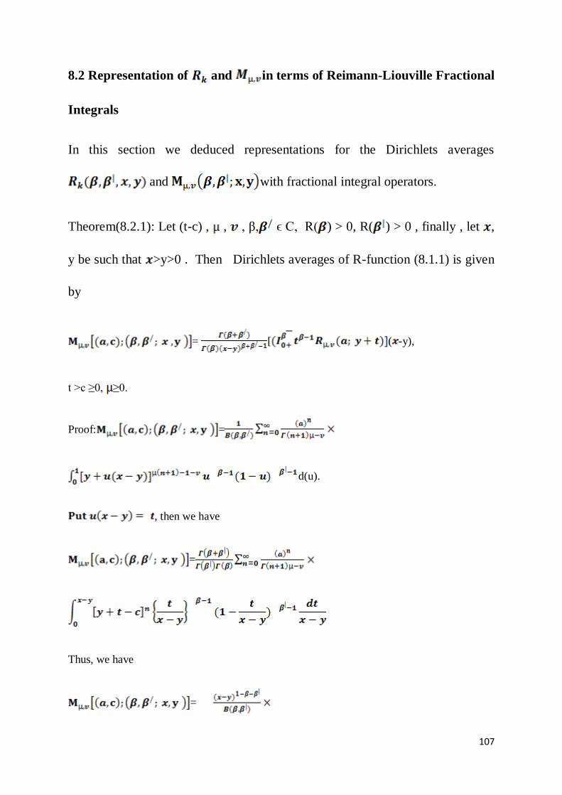
107
8.2 Representation of and in terms of Reimann-Liouville Fractional
Integrals
In this section we deduced representations for the Dirichlets averages
and with fractional integral operators.
Theorem(8.2.1): Let (t-c) , , , β, ϵ C, R( ) > 0, R( ) > 0 , finally , let ,
y be such that >y>0 . Then Dirichlets averages of R-function (8.1.1) is given
by
= [ ( -y),
t >c ≥0, ≥0.
Proof: =
d(u).
, then we have
=
Thus, we have
=
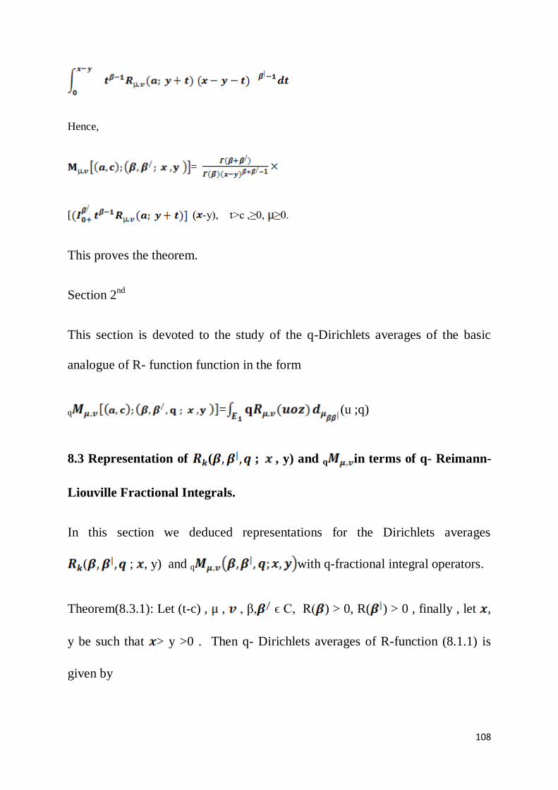
108
Hence,
=
[ ( -y), t>c ,≥0, ≥0.
This proves the theorem.
Section 2nd
This section is devoted to the study of the q-Dirichlets averages of the basic
analogue of R- function function in the form
q = (u ;q)
8.3 Representation of ( ; , y) and q in terms of q- Reimann-
Liouville Fractional Integrals.
In this section we deduced representations for the Dirichlets averages
( ; , y) and q with q-fractional integral operators.
Theorem(8.3.1): Let (t-c) , , , β, ϵ C, R( ) > 0, R( ) > 0 , finally , let ,
y be such that > y >0 . Then q- Dirichlets averages of R-function (8.1.1) is
given by

109
q =
[ ( -y),t >c ≥ 0, ≥0.
Proof: =
(u).
, then we have
q =
Thus, we have
q =
Hence,
q =
[ ( -y), t>c ,≥ 0, ≥0.
This proves the theorem.

110
8.4 Special Cases
Here we consider some particular cases of the above theorem by setting
= -1, c= 0, we get Dirichlets averages of Mittag- Leffler function reported
[9]
( )= .
( ) = .
Further, by setting y= 0 in above equations, we get well- known result reported
in
[8&5] which is as follows
( ) = .
In particular, when = γ, so that
( ) = .
8.5 Conclusion
This chapter has presented a new function for the fractional calculus; it is called
the R-function. The R-function is unique in that it contains all of the derivatives
and integrals of the F-function. The R-function has the Eigen–property that is it

111
returns itself on qth
order differ-integration. Special cases of the R-function also
include the exponential function, the sin, cosine, hyperbolic sine and hyperbolic
cosine functions.
The value of the R-function is clearly demonstrated in the dynamic
thermocouple problem where it enables the analyst to directly inverse transform
the Laplace domain solution, to obtain the time domain solution.
Reference
[1]. Carlson.B.C. (1963), Lauricella‟s hypergeometric function FD, J. Math. Anal. Appl. 7, pp.
452-470.
[2]. Carlson.B.C. (1969), A connection between elementary and higher transcendental functions,
SIAM J. Appl. Math. 17, No. 1 pp. 116-148.
[3]. Carlson.B.C. (1977), Special Functions of Applied Mathematics, Academic Press, New York.
[4]. Carlson.B.C. (1991), B-splines, hypergeometric functions and Dirichlets average, J. Approx.
Theory 67, pp. 311-325.
[5]. Samko S.G, Kilbas A.A, Marichev O.I(1993), Fractional integrals and derivatives, theory and
applications Gordon and Brench , New York et al.
[6]. Hartley, T.T. and Lorenzo, C.F. (1998) , A solution to the fundamental linear fractional order
differential equation , NASA\TP-20863\REVI, December 1998.
[7]. Lorenzo. C.F, Hartley. T.T (1999), Generalized Functions for the Fractional Calculus;
NASA\TP-1999-209424\REVI.
[8]. Kilbas.A.Aand kattuveettil. A (2008),Representations of the Dirichlets averages of the
generalized Mittag-Leffler function via fractional integrals and special functions. Fractional
Calculus & Applied analysis, Vol (11).
[9]. Saxena. R.K, Pogany.T.K, Ram .J and Daiya.J (2010), Dirichlets averages of generalized
multi-index Mittag-Leffler functions.Armenian journal of Mathematics Vol (3) No.4, pp. 174-
187.


![HYPERGEOMETRIC FUNCTIONS IarXiv:1309.4568v1 [math.CA] 18 Sep 2013 HYPERGEOMETRIC FUNCTIONS I IAN G. MACDONALD Contents Foreword 1 1. 2 2. Particular cases 4 3. Integral formulae 7](https://img.dokumen.tips/doc/110x75/5e2f371461b5076fc4686c08/hypergeometric-functions-i-arxiv13094568v1-mathca-18-sep-2013-hypergeometric.jpg)