Basic controller tuning for large offshore wind · PDF file154 K. O. Merz: Basic controller tuning for large offshore wind turbines The ﬂexibility and aerodynamic response of a real

Wind Energ. Sci., 1, 153–175, 2016www.wind-energ-sci.net/1/153/2016/doi:10.5194/wes-1-153-2016© Author(s) 2016. CC Attribution 3.0 License.

Basic controller tuning for large offshore wind turbines

Karl O. MerzSINTEF Energy Research, Sem Sælandsvei 11, 7034 Trondheim, Norway

Correspondence to: Karl O. Merz ([email protected])

Received: 26 April 2016 – Published in Wind Energ. Sci. Discuss.: 19 May 2016Accepted: 12 August 2016 – Published: 29 September 2016

Abstract. When a wind turbine operates above the rated wind speed, the blade pitch may be governed by abasic single-input–single-output PI controller, with the shaft speed as input. The performance of the wind turbinedepends upon the tuning of the gains and filters of this controller. Rules of thumb, based upon pole placement,with a rigid model of the rotor, are inadequate for tuning the controller of large, flexible, offshore wind turbines.It is shown that the appropriate controller tuning is highly dependent upon the characteristics of the aeroelasticmodel: no single reference controller can be defined for use with all models. As an example, the ubiquitousNational Renewable Energy Laboratory (NREL) 5 MW wind turbine controller is unstable when paired witha fully flexible aeroelastic model. A methodical search is conducted, in order to find models with a minimumnumber of degrees of freedom, which can be used to tune the controller for a fully flexible aeroelastic model;this can be accomplished with a model containing 16–20 states. Transient aerodynamic effects, representingrotor-average properties, account for five of these states. A simple method is proposed to reduce the full transientaerodynamic model, and the associated turbulent wind spectra, to the rotor average. Ocean waves are also animportant source of loading; it is recommended that the shaft speed signal be filtered such that wave-driventower side-to-side vibrations do not appear in the PI controller output. An updated tuning for the NREL 5 MWcontroller is developed using a Pareto front technique. This fixes the instability and gives good performance withfully flexible aeroelastic models.

1 Introduction

Much of the research on wind energy systems is based onreference wind turbines, including descriptions of the aero-dynamics, structures, and controls. These reference turbinesare implemented in a variety of models, from high-resolution3-D geometry for CFD/FEM to models containing just a fewdegrees of freedom for electrical grid analysis. A consistentimplementation of the controls is of the utmost importance:few aspects of wind turbine or wind power plant dynamicscan be studied without considering the controls. Yet there isa sensitive interdependence between the controller and theaeroelastic properties of the wind turbine model. In general,the same controller will not produce the same closed-loopdynamic response on models of different fidelities. If the re-sponses differ in important respects such as power fluctua-tions, rotor loads, pitch activity, and stability, then the modelsare, in essence, not of the same wind turbine.

It is often taken for granted that a 1 or 2 degree-of-freedomdrivetrain model, with pole-placement techniques, will pro-vide a reasonable gain tuning for the controller of a windturbine. Hansen et al. (2005) describe such a gain tuning andscheduling approach where the target for the rotor speed con-trol mode – that is, the mode which appears above the ratedwind speed, where pitching of the blades is used to hold therotor speed near a constant target value – has a natural fre-quency of 0.1 Hz and damping ratio of 0.66. The gains arescheduled on the basis of a single parameter: ∂Pa/∂β, thesensitivity of the aerodynamic power with respect to the col-lective blade pitch angle. This same approach was adoptedby Jonkman et al. (2009) in the design of the control sys-tem for the ubiquitous National Renewable Energy Labora-tory (NREL) 5 MW reference wind turbine, which is still thebaseline for much of the research on utility-scale wind en-ergy systems.

Published by Copernicus Publications on behalf of the European Academy of Wind Energy e.V.

154 K. O. Merz: Basic controller tuning for large offshore wind turbines

The flexibility and aerodynamic response of a real windturbine have a strong influence on the rotor speed controlmode. If the gains are not adapted accordingly, the actualmode will have a response which differs significantly fromthe target frequency and damping ratio. This fact is well-known, also to those authors who have employed the sim-plistic gain-tuning approaches. The performance of the windturbine is subsequently verified by aeroelastic simulations,and if the control system performs reasonably from an engi-neering standpoint, it may be considered a successful design.

There are problems with this approach, though. One or twodegree-of-freedom models provide little insight into the truedynamics of the system: essentially, the controller tuning isbeing conducted blindly. The resulting behavior of the rotorspeed control mode depends strongly upon the properties ofthe aeroelastic model, so the same controller may functionwell or poorly, in a given application. Users of the controllermay not understand, or acknowledge, the limitations.

For example, the NREL 5 MW proportional-integral (PI)controller is often adopted as the baseline for com-parison against advanced control algorithms: see Schlipfet al. (2013), Spencer et al. (2013), Jafarnejadsani andPieper (2014), and Yang et al. (2015) for some recent exam-ples. Yet this controller is unstable when paired with a fullyflexible aeroelastic model which includes elastic twisting ofthe blades. For a fair comparison, the reference PI controllershould be tuned according to the same model and criteriathat were used to demonstrate the performance of the opti-mal control algorithms; failure to do so weakens the scientificbasis of the results.

Controller tuning does not need to be based on a reducedmodel. Tibaldi et al. (2012) optimized the gains of bladepitch and generator torque controllers using full aeroelasticload simulations, combined with a component cost model.The optimization, which ran through seven iterations, wasnoted to require 4000 h computing time, which limits practi-cability of the method. Nonetheless, the approach of Tibaldiet al., considering the influence of loads and energy produc-tion on lifetime cost, is the proper way to evaluate the overallperformance of a wind turbine control system.

A practical model for control design contains a minimalnumber of degrees of freedom. It is reasonable to use a low-fidelity model, since a well-designed controller will be robustto small inaccuracies associated with neglected higher-ordereffects. The model must be of sufficient resolution to capturethe important first-order effects. In particular, the frequen-cies and damping ratios of the control-dominated closed-loopmodes within the full model should be preserved in the sim-ple model.

There is not a perfect consensus on which degrees of free-dom must be included in a model for control design. Amongolder publications, Leithead and Connor (2000) is a goodplace to start, as they conclusively demonstrated that rigid-body models of the drivetrain are inadequate. They includedthe response of the rotor aerodynamic torque to perturba-

tions in the rotational speed, blade pitch angle, and rotor-average wind speed: ∂Ta/∂�,∂Ta/∂β, and ∂Ta/∂u, respec-tively. Generator dynamics were also included, as third-ordertransfer functions, but the blades and tower were consideredrigid. Bossanyi (2000), without providing a formal justifica-tion, listed the minimal degrees of freedom for design of theblade pitch controller. The list includes rotor rotation, drive-train torsion, and tower fore–aft motion as the structural de-grees of freedom; flexibility of the blades was omitted. LikeLeithead and Connor, Bossanyi recommended including gen-erator dynamics but also added pitch actuator and speed sen-sor dynamics.

Wright (2004) conducted a methodical investigation intothe structural degrees of freedom necessary to obtain a stablecontrol tuning. The 600 kW, 42.6 m diameter CART (Con-trols Advanced Research Turbine) was used as a referencecase. A brief, initial investigation demonstrated the impor-tance of drivetrain flexibility and actuator dynamics for areference PI controller. A more extensive degree-of-freedomstudy was conducted with a disturbance-accommodatingcontrol (DAC) strategy, which is a state-feedback control al-gorithm where additional states are used to model, and even-tually cancel, disturbances such as turbulence. Though DACand PI controllers are not identical, lessons learned about theinfluence of structural flexibility on a DAC controller canlikely be applied to PI tuning as well.

Wright progressively activated one structural degree offreedom at a time: drivetrain torsion, collective blade flap,and tower fore–aft. For each set of active degrees of freedom,a controller was synthesized and subsequently evaluated bya brief time-domain simulation with a stepped wind speedprofile. It was found that the first blade-flap-wise modes havethe potential to destabilize the first drivetrain mode and mustbe included in models for control design. The tower modes,principally the first fore–aft mode, were found not to have asignificant influence on the behavior of the rotor speed con-trol.

Sønderby and Hansen (2014) revisited the question ofwhich degrees of freedom should be included in a controltuning model, in the context of an onshore version of theNREL 5 MW wind turbine. The controller was not speci-fied; rather, the investigation was based on open-loop transferfunctions between the actuated degrees of freedom – collec-tive blade pitch and generator torque – and generator speed.Particular emphasis was placed on how the poles (indicatingfrequency and damping properties) associated with the struc-tural modes changed with the activated structural and aero-dynamic degrees of freedom. Capturing the non-minimum

Wind Energ. Sci., 1, 153–175, 2016 www.wind-energ-sci.net/1/153/2016/

K. O. Merz: Basic controller tuning for large offshore wind turbines 155

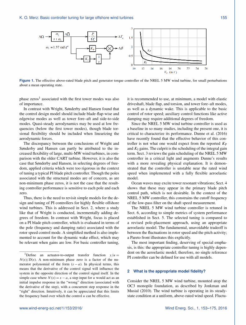
Figure 1. The effective above-rated blade pitch and generator torque controller of the NREL 5 MW wind turbine, for small perturbationsabout a mean operating state.

phase zeros1 associated with the first tower modes was alsoof importance.

In contrast with Wright, Sønderby and Hansen found thatthe control design model should include blade-flap-wise andedgewise modes as well as tower fore–aft and side-to-sidemodes. Quasi-steady aerodynamics may be used at low fre-quencies (below the first tower modes), though blade tor-sional flexibility should be included when linearizing theaerodynamic forces.

The discrepancy between the conclusions of Wright andSønderby and Hansen can partly be attributed to the in-creased flexibility of large, multi-MW wind turbines, in com-parison with the older CART turbine. However, it is also thecase that Sønderby and Hansen, in selecting degrees of free-dom, applied criteria which were too rigorous in the contextof tuning a typical PI blade pitch controller. Though the polesassociated with the structural modes are of concern, as arenon-minimum phase zeros, it is not the case that the result-ing controller performance is sensitive to each pole and eachzero.

Thus, there is the need to revisit simple models for the de-sign and tuning of PI controllers for highly flexible offshorewind turbines. This is addressed in Sect. 2, where a studylike that of Wright is conducted, incrementally adding de-grees of freedom. In contrast with Wright, focus is placedon a PI blade pitch controller, which is evaluated in terms ofthe pole (frequency and damping ratio) associated with therotor speed control mode. A simplified method is also imple-mented to account for the dynamic wake effect, which maybe relevant when gains are low. For basic controller tuning,

1Define an actuator-to-output transfer function y/u=

N (s)/D(s). A non-minimum phase zero is a factor of the nu-merator polynomial of the form (s− a). In physical terms, thismeans that the derivative of the control signal will influence thesystem in the opposite direction of the control signal itself. In thesimple case where N (s)= s− a, a step input for u would act as aninitial impulse response in the “wrong” direction (associated withthe derivative of the step), with a concurrent step response in the“right” direction. Intuitively, it can be appreciated that this limitsthe frequency band over which the control u can be effective.

it is recommended to use, at minimum, a model with elasticdriveshaft, blade flap, and torsion, and tower fore–aft modes,as well as a dynamic wake. This is applicable to the basiccontrol of rotor speed; auxiliary control functions like activedamping may require additional degrees of freedom.

Since the NREL 5 MW wind turbine controller is used asa baseline in so many studies, including the present one, it iscritical to characterize its performance. Dunne et al. (2016)have recently found that the effective behavior of this con-troller is not what one would expect from the reported KPandKI gains. The culprit is the scheduling of the integral gainterm. Sect. 3 reviews the gain scheduling of the NREL 5 MWcontroller in a critical light and augments Dunne’s resultswith a more revealing physical explanation. It is demon-strated that the controller is unstable near the rated windspeed when implemented with a fully flexible aeroelasticmodel.

Ocean waves may excite tower resonant vibrations; Sect. 4shows that these may appear in the primary blade pitchcontrol path, which is not desirable. In the context of theNREL 5 MW controller, this constrains the cutoff frequencyof the low-pass filter on the shaft speed measurement.

The NREL 5 MW wind turbine controller is retuned inSect. 6, according to simple metrics of system performanceestablished in Sect. 5. The selected tuning is compared toa revised pole-placement approach, using an appropriateaeroelastic model. The fundamental, unavoidable tradeoff isbetween the fluctuations in rotor speed and the pitch activity;a Pareto front illustrates this explicitly.

The most important finding, deserving of special empha-sis, is this: the appropriate controller tuning is highly depen-dent on the aeroelastic model; therefore, no single referencePI controller can be defined for use with all models.

2 What is the appropriate model fidelity?

Consider the NREL 5 MW wind turbine, mounted atop theOC3 monopile foundation, as described by Jonkman andMusial (2010). The wind turbine is operating in its steady-state condition at a uniform, above-rated wind speed. Fluctu-

www.wind-energ-sci.net/1/153/2016/ Wind Energ. Sci., 1, 153–175, 2016


ations in the wind speed are, at present, limited to small per-turbations about the mean. In this case, the rotor speed andgenerator power output are controlled as shown in Fig. 1. (Allspeeds are given in reference to the low-speed shaft. The gainscheduling in Fig. 1 differs from the controller described byJonkman et al. (2009), for reasons which are made clear inSect. 3.)

It is desirable to ask some basic questions about this con-troller. How well does it perform? Could the gains and low-pass filter be chosen differently, to improve the performance?Is the same controller tuning also applicable to an offshorewind turbine? These are the topics of Sects. 4–6. In order toarrive at the answers, a model of the closed-loop system dy-namics is needed. This could be a high-resolution model. Yetthere are advantages in adopting a simple model. A simplemodel is computationally efficient, aids understanding of thesystem behavior, and can form the basis for more advancedstate-space control algorithms. In light of inconsistencies inthe literature regarding which degrees of freedom are needed,it is worthwhile to establish some minimum requirements fora model of the closed-loop system dynamics.

2.1 The rotor speed control mode

With the use of a multiblade coordinate transform, a three-bladed wind turbine operating under normal conditions (bal-anced rotor, no extreme excursions) can be represented as alinear time-invariant system, with state and output equationsof the form

Ldx

dt= Ax+Bu and y = Cx+Du. (1)

Hansen (2004) and van Engelen and Braam (2004) describeprograms which model wind turbines in this manner; van En-gelen and van der Tempel (2004), Merz (2015a), and Tibaldiet al. (2015) have extended the scope of linear state-spaceanalysis to the computation of loads under turbulent windconditions. The present results are obtained using the windturbine module of the STAS program, which is documentedin a series of technical memos (Merz 2015b, c, d). The ap-proach is broadly similar to that of Hansen or van Engelenand does not warrant a detailed presentation here.

In the discussion that follows we must distinguish betweentwo categories of modes. STAS employs modal reduction ofeach body (tower, nacelle, driveshaft, and the three blades)prior to assembling the bodies, via constraint equations, intothe full wind turbine. For instance, the amplitudes of the firstfore–aft and side-to-side modes of the tower body (includingthe foundation and soil p–y springs) are denoted qF and qS,respectively. These body modes are degrees of freedom inthe equations of motion; they are elements in the state vectorx, as are their time derivatives dqF/dt and dqS/dt . The bodymodes may incorporate features such as bend–twist couplingof the blades.

The second class of modes is the eigenvectors of the equa-tions of motion of the assembled structure, including systemssuch as the generator, pitch actuators, and controls. Thesesystem modes may be dominated by one body mode – for in-stance, there is an obvious “first tower fore–aft” system mode– or they may have complicated shapes which are not so eas-ily described.

Representing the wind turbine in the form of Eq. (1), themodal properties of the system can be computed. An exami-nation of the system modes reveals one primary and one sec-ondary mode, which, within reasonable bounds of the gaintuning, contain the dominant action of the controller. Theprimary mode can be called the “rotor speed control” mode,as it represents the fluctuation in the rotational speed of thewind turbine rotor, under the combined control actions of thegenerator and blade pitch actuators. The secondary mode isassociated with the influence of dynamic wake effects on therotor speed control; this will be called the “dynamic wake”mode. It is most active when control gains are set to compar-atively low values.

There is overlap between the rotor speed control and dy-namic wake modes. The rotor speed control mode containsthe dominant rotor speed and blade pitch responses, but thestates associated with the dynamic wake – the induced ve-locities – also participate. The dynamic wake mode containsthe dominant response of the rotor-wide collective inducedvelocities, but these are driven by changes in the rotor speedand blade pitch, which also appear in this mode. Thus, theparticipation of the dynamic wake in the rotor speed controlmode is not to be confused with the influence of the dynamicwake mode on the rotor speed and blade pitch response. Theformer is a dominant effect, which is addressed in Sect. 2.2.The latter, it will be shown shortly, is not so relevant, exceptwhen control gains are lower than usual. The salient point isthat a dynamic wake model may be needed, even if the dy-namic wake mode makes little contribution to the responseof the relevant control variables.

The rotor speed control mode is clearly visible in transferfunctions between axial wind speed and rotor speed. Figure 2shows these transfer functions, as well as those for bladepitch, at four wind speeds between rated and cut-out. Theseresults were obtained for a full (ca. 600 states) model of theNREL 5 MW wind turbine on a flexible tower and founda-tion, including soil flexibility.

Figure 2 also lists the natural frequency and damping ra-tio of the rotor speed control mode. The natural frequency isassociated with the peak in the rotor speed transfer function,while the damping ratio indicates to some extent the sharp-ness of the peak. Although the rotor speed control mode isdominant, several other system modes also participate in theresponse.

To keep things simple, the discussion of model fidelity isfocused on the two system modes with the greatest contri-bution to the low-frequency rotor speed response. For thebaseline gains of Fig. 1, typical participation factors (Kun-



Figure 2. Closed-loop transfer functions of collective blade pitch (gray lines) and rotor speed (black lines) with respect to a uniformsinusoidal perturbation in the axial wind speed. Angular units are radians. Note the different y axis scale of the upper-left plot.

Figure 3. Magnitudes (left) and phases (right) of transfer functions between axial wind speed and blade pitch, rotor speed, and tower mudline bending moments. Three gains are shown: 0.5, 1.0 (thick lines), and 1.5 times the baseline gains from Fig. 1. The natural frequency (Hz)and damping ratio of the rotor speed control (1) and dynamic wake (2) modes are also shown, tabulated as a function of the gain multiple.

dur, 1994) associated with the rotor rotational degree of free-dom are 0.5 for the dominant rotor speed control mode and0.2 for the secondary dynamic wake mode. These two modesserve as surrogates for the full transfer function: the proper-ties of the transfer function, within the region influenced bythe control tuning, can be inferred from the properties of themodes.

As an example, let the NREL 5 MW turbine, on the OC3monopile foundation, be operating at a mean wind speed of16 m s−1. The baseline gains from Fig. 1 are now modifiedby a factor α:

KP = αKP0 and KI = αKI0. (2)

Figure 3 plots the transfer functions of blade pitch, rotorspeed, and tower mud line bending moments, with respect toa uniform fluctuation in the axial wind speed. The frequencyand damping properties of the rotor speed control and dy-namic wake modes are tabulated as a function of the gainmultiple. At high gains, the peak in the rotor speed transferfunction is dominated by the rotor speed control mode, whileat low gains, both the rotor speed control and dynamic wakemodes make significant contributions.

There is evidently a minimum in the peak sensitivity of ro-tor speed to fluctuating winds. At high gains, the blade pitchresponds aggressively, in a manner which reduces the damp-ing of the rotor speed control mode, while at low gains, the



Figure 4. On the left: normalized spectra of the collective component of rotationally sampled axial turbulence (V∞ = 16 m s−1, I = 0.15)at r/R = 0.75 and ocean wave loads with Hs = 2 m and Tp = 6 s. On the right: spectra of tower bending moments at the mud line, for gainmultiples of 0.5, 1.0 (thick line), and 1.5. (The three curves associated with the side-to-side spectra overlap.)

blade pitch response is so passive that it does not promptlyarrest perturbations to the rotor speed.

Within reasonable bounds, gain tuning has little influenceon the resonant response of the tower. This is mainly dueto the non-minimum phase zero at 0.236 Hz. The presenceof this zero is associated with the first tower fore–aft bodymode. The nacelle moves in such a manner that the mea-sured fluctuation in shaft speed is near zero, and there is thusno control response. The particular characteristics of the zeroare influenced by other body modes, as well as where in thedrivetrain the shaft speed is measured. In the most basic casewhere the only elastic degree of freedom is the tower fore–aftmotion, the zero is caused by nacelle fore–aft motion whichnearly cancels the fluctuating wind speed. When all the elas-tic degrees of freedom are included, the motion at the fre-quency of the zero defies such a simple description, but theoutcome is similar.

The controller influence at higher frequencies is sup-pressed by the low-pass filter, with a corner frequency of0.25 Hz.

The response of the wind turbine depends on both theinput–output transfer functions, as in Fig. 2, and the charac-teristics of the environmental inputs. Typical spectra of rota-tionally sampled atmospheric turbulence (the collective com-ponent at an outboard blade station) and ocean wave forcesare plotted on the left side of Fig. 4. Most of the energy inthe turbulence is concentrated at low frequencies, while thatof the ocean waves is in the vicinity of 1/Tp, where Tp is thepeak in the wave elevation spectrum.

The right-hand side of Fig. 4 shows spectra of the towermud line bending moments, for three values of the gain mul-tiple α. The peak in the response at low gains is due to thegreater energy in the turbulence at low frequencies, while thepeak at high gains is due to reduced damping of the rotorspeed control mode. (The peak at a gain multiple of 1.5 isnot caused by interaction between the controller and oceanwaves; Sect. 4 contains further discussion on this point.) Inthe present example, the baseline gains find a happy middleground. Though not visible in the figure, the response spec-

tra above 0.3 Hz are essentially unaffected by the choice ofgains.

To sum up: if we know the natural frequency and dampingratio of the rotor speed control and dynamic wake modes, wecan infer much about the response of the wind turbine to thecontrol actions. For a reduced model to be useful in tuninggains, a minimal requirement is that it is able to correctlypredict the properties of the rotor speed control mode. If lowgains are to be evaluated – for instance, if the rotor speed con-trol mode might be placed below the ocean wave frequencyband – then it is also needed to predict the properties of thedynamic wake mode.

The above statements are valid in the context of basic rotorspeed control, for a wind turbine operating above the ratedwind speed. Additional control functions – say, active damp-ing of tower or drivetrain resonance – may require that addi-tional system modes are also correctly predicted.

2.2 The importance of transient aerodynamic loads

Aerodynamic forces on the blades are subject to transientsas conditions change, with a particularly strong effect associ-ated with the blade pitch angle. The transients can be groupedinto the categories of circulation lag (Theodorsen), associ-ated with the development of lift along the blade; dynamicstall, connected with movement of the chordwise location offlow separation; and dynamic wake (or dynamic inflow), re-lated to the downstream convection of vorticity in the wake,which governs the induced velocity at the rotor plane. In ananalysis with the blade element momentum method, thesephenomena can be represented by a set of linear differentialequations, associated with each blade element. The equationsemployed here are based on the circulation lag method de-scribed by Leishman (2002) and also Hansen et al. (2004);the Merz et al. (2012) variant of the Øye (1990) dynamicstall model; and Øye’s dynamic wake model, as documentedby Snel and Schepers (1995). Neglecting the tangential com-ponent of induced velocity, the aerodynamic state equations



Figure 5. Closed-loop transfer functions of collective blade pitch (thin lines) and rotor speed (thick lines) with respect to a uniform sinusoidalperturbation in the axial wind speed. Nonlinear time-domain computations using FAST v8 are compared to equivalent results from a linearstate-space model, obtained using equilibrium and dynamic wakes. The FAST results should be compared to the equilibrium-wake (black)curves.

associated with a given blade element are

ddt

v̂iviαda1a2

=−τ−1

1 0 0 0 0τ−1

2 τ−12 0 0 0

0 0 −τ−1 τ−1K1 τ−1K20 0 0 0 10 0 0 A54 A55

v̂iviαda1a2

+

0.4τ−11 0

0.6τ−12 0

0 τ−1K30 00 1

[viqαq

], (3)

with

A54 =−b1b2

(2Vc

)2

, A55 =− (b1+ b2)(

2Vc

),

K1 = (A1+A2)b1b2

(2Vc

)2

K2 = (A1b1+A2b2)(

2Vc

), K3 = (1−A1−A2) ,

A1 = 0.165, A2 = 0.335, b1 = 0.0455,

b2 = 0.3, τ1 =1.1

1− 1.3a

(D

2V∞

), a =

vi

V∞,

τ2 =

[0.39− 0.26

(2rD

)2], and τ = 4.3

c

V.

The five states are an intermediate induced velocity variablev̂i, the induced velocity vi, the dynamic angle-of-attack αd,and two intermediate angle-of-attack variables a1 and a2.The incoming wind speed is V∞, while V is the local rel-ative wind speed at the airfoil, c is the chord length, r is theradial location, andD is the rotor diameter. The quasi-steadyinduced velocity viq and angle-of-attack αq are computed as-suming instantaneous wake development. Angles are in radi-ans, and all quantities are given in standard SI units.

An examination of the A matrix in Eq. (3) shows thatthe first two states, which represent the dynamics of the ro-tor wake, are not directly coupled with the remaining threestates, which represent the circulatory flow local to the air-foil. The dynamic wake and “circulation” effects are inter-dependent when linked to the full state-space model of thewind turbine, but they can be independently activated or de-activated.

Considering first the dynamic wake, Fig. 5 shows trans-fer functions of rotor speed and blade pitch with respect torotor-average wind speed. The solid curves were computed inthe frequency domain, based upon a linear state-space model.Two cases are shown, one with the dynamic wake model ac-tive, and another with it inactive, such that the induced ve-locities are always in equilibrium with the airfoil forces.



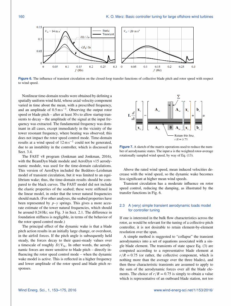
Figure 6. The influence of transient circulation on the closed-loop transfer functions of collective blade pitch and rotor speed with respectto wind speed.

Nonlinear time-domain results were obtained by defining aspatially uniform wind field, whose axial velocity componentvaried in time about the mean, with a prescribed frequency,and an amplitude of 0.5 m s−1. Observing the output rotorspeed or blade pitch – after at least 30 s to allow startup tran-sients to decay – the amplitude of the signal at the input fre-quency was extracted. The fundamental frequency was dom-inant in all cases, except immediately in the vicinity of thetower resonant frequency, where beating was observed; thisdoes not impact the rotor speed control mode. Time-domainresults at a wind speed of 12 m s−1 could not be generated,due to an instability in the controller, which is discussed inSect. 3.4.

The FAST v8 program (Jonkman and Jonkman, 2016),with the BeamDyn blade module and AeroDyn v15 aerody-namic module, was used for the time-domain calculations.This version of AeroDyn included the Beddoes–Leishmanmodel of transient circulation, but it was limited to an equi-librium wake; thus, the time-domain results should be com-pared to the black curves. The FAST model did not includethe elastic properties of the seabed; these were stiffened inthe linear model, in order that the tower natural frequenciesshould match. (For other analyses, the seabed properties havebeen represented by p–y springs. This gives a more accu-rate estimate of the tower natural frequencies, which shouldbe around 0.24 Hz; see Fig. 3 in Sect. 2.1. The difference infoundation stiffness is negligible, in terms of the behavior ofthe rotor speed control mode.)

The principal effect of the dynamic wake is that a bladepitch action results in an initially large change, or overshoot,in the airfoil forces. If the pitch angle is subsequently heldsteady, the forces decay to their quasi-steady values overa timescale of roughly D/V∞. In other words, the aerody-namic forces are more sensitive to blade pitch – directly in-fluencing the rotor speed control mode – when the dynamicwake model is active. This is reflected in a higher frequencyand lower amplitude of the rotor speed and blade pitch re-sponses.

Figure 7. A sketch of the matrix operations used to reduce the num-ber of aerodynamic states. The input u is the weighted rotor-averagerotationally sampled wind speed, by way of Eq. (13).

Above the rated wind speed, mean induced velocities de-crease with the wind speed, so the dynamic wake becomesless significant at higher mean wind speeds.

Transient circulation has a moderate influence on rotorspeed control, reducing the damping, as illustrated by thetransfer functions in Fig. 6.

2.3 A (very) simple transient aerodynamic loads modelfor controller tuning

If one is interested in the bulk flow characteristics across therotor, as would be relevant for the tuning of a collective pitchcontroller, it is not desirable to retain element-by-elementresolution over the span.

A simple method is suggested to “collapse” the transientaerodynamics into a set of equations associated with a sin-gle blade element. The transients of state space Eq. (3) arecomputed according to a representative blade element atr/R = 0.75 (or rather, the collective component, which isnothing more than the average over the three blades), andthen these characteristic transients are assumed to apply tothe sum of the aerodynamic forces over all the blade ele-ments. The choice of r/R = 0.75 is simply to obtain a valuewhich is representative of an outboard blade station, not too



close to the tip. The results are not sensitive to the preciseradial location.

It is perhaps easiest to explain this operation by sketchingthe process by which the aerodynamic states are reduced, asin Fig. 7. For simplicity, this is presented as if there were onlyone aerodynamic state associated with each blade element;the process is identical for each of the five types of states inEq. (3). In the state vector, there is a group xs with the struc-tural states, a group xa with the aerodynamic states, and agroup xc with the control states. The parts shaded gray, as-sociated with the aerodynamic states, are partitioned out anddeleted. Only one aerodynamic state is retained, that associ-ated with the collective component at r/R = 0.75. Its row,shown as a black line, is unchanged (apart from the deletedcolumns). However, in the rows of the A matrix associatedwith the structural states, the columns associated with theaerodynamic states (light gray) are summed into the columnof the retained aerodynamic state (white bar). In this manner,the transient evolution of the single retained aerodynamicstate comes to represent the response over the entire rotor.(The L matrix is also modified, but as the only nonzero ele-ments in the relevant rows and columns lie on the diagonal,the operation is trivial.)

The process is repeated for each of the five types of aero-dynamic states in Eq. (3), and the result is that five statesrepresent the collective, transient aerodynamics of the rotor.

There are other, more formal methods by which the num-ber of aerodynamic states could be reduced. A low-order se-ries representation of rotor induction, such as the accelera-tion potential method described by Burton et al. (2001), isone possibility. Another is the modal reduction approach ofSønderby (2013) though as derived, this did not include adynamic wake.

Nonetheless, the above ad hoc matrix reduction methodworks well for the present purpose of control tuning, wherelow-frequency, rotor-average wind inputs are of greatestconcern. The reduced model is validated, in Table 1 andSect. 5, against the original matrices employing the fullradius-dependent Øye model of Eq. (3).

2.4 Degrees of freedom

A series of models was constructed, progressing from thesimplest case with only rigid-body rotation of the rotor,through to the full case with the elastic structure representedby 110 modal degrees of freedom. The reduced models em-ployed either quasi-steady aerodynamics or the five-statetransient model of Sect. 2.3, whereas the full model em-ployed a blade element momentum method with transientscomputed for each element. For the reduced models, thenumber of states Ns consists of one state for rotor rotation,two for each elastic degree of freedom, two for the controller,and five for transient aerodynamics. Blade pitch is directlyprescribed by the controller. The full model includes addi-

tional states describing the blade pitch response, as well asthe electrical dynamics of the generator (Merz, 2015d).

Table 1 lists the models. For each model, the natural fre-quency and damping ratio of the rotor speed control modewere computed at three above-rated wind speeds: 12, 16, and20 m s−1. Here the baseline gains of Fig. 1, correspondingto α = 1 in Eq. (2), were used. At this level of gain, the dy-namic wake mode was highly damped, with a damping ra-tio of nearly unity. To better illustrate this mode, and verifythat it was well-predicted where it matters, its properties werecomputed again using a reduced gain factor of α = 0.5. The“correct” result is taken to be that obtained with the full linearmodel, highlighted in bold.

The conclusion is that models which do not include atleast tower fore–aft, blade-flap-wise, and torsional flexibil-ity may give misleading estimates of the rotor speed con-trol response and are therefore unfit for the purpose of tuningthe controller. With blade flap and torsion, tower fore–aft,and a five-state transient aerodynamic model, the rotor speedcontrol and dynamic wake modes are well-predicted. Addingblade edge and tower side-to-side flexibility makes little dif-ference. Model 5D is therefore recommended as a minimalmodel for controller gain tuning.

Drivetrain torsional flexibility is expected to have little in-fluence on the basic control tuning, provided that the low-pass filter frequency is reasonably low; however, this degreeof freedom is retained in the models as it is common prac-tice. It is indeed important to evaluate the damping of thefirst drivetrain mode, as this can potentially be destabilizedby the generator torque control. Model 7D is recommendedfor evaluating the first drivetrain torsional resonance mode,as this is influenced by the flexibility of the blade edgewiseand tower side-to-side modes.

It is emphasized that other control functions which arenot shown in Fig. 1 may require additional degrees of free-dom. Incorporating environmental inputs such as misalignedocean waves may also require additional degrees of freedom,at least those of Model 7D.

As an alternative to an incremental study like that of Ta-ble 1, formal model-reduction methods could be employed,for instance Zhou et al. (1996).

3 Revisiting a baseline control architecture

The nonlinear, gain-scheduled NREL 5 MW wind turbinecontroller, during operation above the rated wind speed, isshown in Fig. 8. The rate limits, pitch angle limits, and inte-gral gain saturation are omitted. With the exception of the 0◦

minimum pitch angle, these limits are seldom reached duringnormal operating conditions. The pitch angle hits 0◦ whenthe wind speed dips below the rated value, and the controlmode transitions between constant-power and constant tip-speed ratio (maximum CP) operation. This transition is not



Table 1. Natural frequencies and damping ratios of the rotor speed control mode (using the baseline gains) and dynamic wake mode(at half the baseline gains), obtained from models with various degrees of freedom (DOFs). Results obtained with the reference high-fidelity model are highlighted in bold. Model 5D is recommended as a minimum model for basic controller gain tuning. Aero indicateswhether the aerodynamics were quasi-steady (QS) or included transient dynamics (Dyn). BEM: blade element momentum method. For otherabbreviations, see the table in Appendix A.

Rotor speed control mode, α = 1.0

12 m s−1 16 m s−1 20 m s−1

ID DOFs Ns Aero f ζ f ζ f ζ

1 R 3 QS 0.0579 0.3336 0.0578 0.5246 0.0474 0.76482 R d 5 QS 0.0580 0.3381 0.0578 0.5267 0.0472 0.76643e R d e 7 QS 0.0580 0.3385 0.0579 0.5240 0.0476 0.76383fc R d f 7 QS 0.0546 0.2068 0.0602 0.4575 0.0531 0.72833Fd F R d 7 QS 0.0594 0.3152 0.0594 0.5157 0.0487 0.76804 R d f t 9 QS 0.0789 0.2293 0.0746 0.4922 0.0759 0.77175Q F R d f t 11 QS 0.0804 0.1889 0.0782 0.4621 0.0892 0.71015D F R d f t 16 Dyna 0.1321 0.1700 0.1141 0.4753 0.1425 0.52036D S F R d f e 18 Dyna 0.0824 0.4710 0.0656 0.5708 0.0874 0.82127Qe S F R d f e t 15 QS 0.0804 0.1902 0.0782 0.4569 0.0904 0.69397D S F R d f e t 20 Dyna 0.1318 0.1722 0.1128 0.4697 0.1401 0.51248D S F R d f e t2 22 Dyna 0.1360 0.1338 0.1185 0.4248 0.1443 0.4757

Full 572 QS 0.0889 0.1706 0.0847 0.4404 0.1040 0.6295Full 221 Dyna 0.1385 0.1124 0.1215 0.4008 0.1464 0.4560Full 572 Dynb 0.1370 0.1050 0.1211 0.4087 0.1465 0.4618

Dynamic wake mode, α = 0.5

5D F R d f t 16 Dyna 0.0604 0.8445 0.0464 0.6092 0.0172 0.92086D S F R d f e 18 Dyna 0.0477 0.9365 0.0661 0.9297 0.000 > 17D S F R d f e t 20 Dyna 0.0602 0.8450 0.0466 0.6065 0.0171 0.92108D S F R d f e t2 22 Dyna 0.0582 0.8399 0.0479 0.6189 0.0162 0.9282

Full 221 Dyna 0.0563 0.8408 0.0487 0.6280 0.0156 0.9324Full 572 Dynb 0.0521 0.8762 0.0455 0.6455 0.0161 0.9243

R: rigid rotor and blade pitch; d: driveshaft torsion; e: blade edgewise; f: blade-flap-wise; t: blade torsion; F: tower fore–aft; S:tower side to side. Notes: a Reduced rotor-average transient circulation, stall, and wake models: five states. b Full transientcirculation, stall, and wake models using BEM. c The minimum elastic DOFs recommended by Wright (2004). d The minimumelastic DOFs recommended by Bossanyi (2000). e The minimum elastic DOFs recommended by Sønderby and Hansen (2014).

Figure 8. On the left, the equivalent functions of the NREL 5 MW turbine controller during normal, non-saturated operation. The integralpathway (dashed box) contains the scheduled gain outside the integrated speed error. On the right, an alternate integral pathway with thescheduled gain inside the integral of the speed error.



crucial to the present argument and is ignored for the timebeing.

The critical feature to note is that the scheduling of theintegral gain happens outside the integral of the speed error,9. That is, the contribution of the integral pathway to thedemanded blade pitch angle is

KI(β)

t∫0

(�−�r

)dτ. (4)

It will be shown that this leads to a misleading definition ofproportional and integral gain. An alternative is to schedulethe integral gain inside the integral,

t∫0

KI(β)(�−�r

)dτ, (5)

also shown at the right of Fig. 8. In state space, the equationsdescribing the controller are

d

dt

[9

�

]=

[0 10 −ωL

][9

�

]+

[0 −1ωL 0

][��r

](6a)

β =[KI (β) KP (β)

][ 9

�

]+[

0 −KP (β)][ �

�r

], (6b)

where the gain is outside the integral, vs.

d

dt

[9 ′

�

]=

[0 KI (β)0 −ωL

][9 ′

�

]+

[0 −KI (β)ωL 0

][�

�r

](7a)

β =[

1 KP (β)][ 9 ′

�

]+[

0 −KP (β)][ �

�r

], (7b)

where the gain is now inside the integral. A prime is addedto 9 ′, as this is not the same as the integrated speed error 9.

Dunne et al. (2016) identified the fact that by schedulingthe integral gain outside of the accumulated speed error, theeffective gains, for small perturbations about a mean operat-ing point β0, are significantly lower than KP (β) and KI (β).Here this finding is given a deeper physical explanation.

3.1 The role of the integral pathway

For a steady-state operating point, with zero speed error, theintegral pathway provides the mean blade pitch angle setpoint. This is clearly illustrated by observing the behaviorof the controller while the turbine starts up in a condition ofabove-rated wind speed; Fig. 9 is an example. In this sim-ulation, using the FAST v8 program, the wind speed wasa constant 15 m s−1 and the structure was rigid. The ini-tial conditions were a rotor speed equal to the rated speed

Figure 9. Startup of a simulation at a wind speed of 15 m s−1,showing how the steady-state blade pitch angle is set by the integralpathway. The perceptible lag between the integrated speed error,and the integral pathway’s contribution to the blade pitch command,hints at the problem with scheduling the gain outside the integral ofthe speed error.

of 12.1 rpm (in order to avoid implementing specific startupcontrol logic), a blade pitch angle of 0◦, and a low-pass fil-tered speed error and integrated speed error of zero. The fullnonlinear NREL 5 MW controller was employed, includinglimits, although these did not come into effect.

Thus, the integrated error 9 has a comparatively largemean offset when the turbine is operating above the ratedwind speed.

The integral pathway also acts, together with the low-passfilter, to determine the lag between fluctuations in the rota-tional speed and the blade pitch angle, which in turn influ-ences the response of the system. This is best illustrated inthe frequency domain, as in the following section, where theconcept of phase can be applied.

3.2 The effect of scheduling the integral gain

Let the NREL 5 MW wind turbine be operating in a uniform,steady, above-rated wind. Let there be a small perturbationto the shaft speed, 1�, which could be the result of, say,a small fluctuation in the wind speed. The state equation ofthe baseline controller, Eq. (6a), is linear and therefore of thesame form,

d

dt

[19

1�

]=

[0 10 −ωL

][19

1�

]+

[0ωL

]1�, (8a)

for small perturbations. Note that �r is constant and so van-ishes from the perturbation equations. Linearization of thenonlinear gain-scheduled blade pitch output, Eq. (6b), gives

1β =

(1−

∂KI

∂β

∣∣∣∣090

)−1 [KI0 KP0

][ 191�

]. (8b)

As ∂KI/∂β|0 is a negative value and 90 is a positive value,the effective gains which multiply 19 and 1� are smaller



than the respectiveKI0 andKP0. By contrast, linearization ofthe controller of Eq. (7a, b), with the gain scheduling insidethe integral, gives

d

dt

[19

1�

]=

[0 10 −ωL

][19

1�

]+

[0ωL

]1� (9a)

1β =[KI0 KP0

][ 191�

](9b)

after rearranging to replace 9 ′ with 9. It is now argued thatEq. (7a, b), with linearizations (9a, b), are unambiguouslythe correct way to define the behavior of a PI control system.If one looks at the signals coming from the proportional andintegral pathways, for small perturbations about the mean,Eq. (9b) (scheduling inside the integral) gives

1βP =KP01� and 1βI =KI019,

with 1β =1βP+1βI, (10)

which is exactly what is expected. On the other hand,Eq. (8b) (scheduling outside the integral) results in

1βP =KP01� and

1βI =

(1−

∂KI

∂β

∣∣∣∣090

)−1

KI019

+

[(1−

∂KI

∂β

∣∣∣∣090

)−1

− 1

]KP01�. (11)

That is, the signal coming from the integral pathway con-tributes both integral and proportional effects. This is confus-ing, to say the least.

The behavior of the two versions of the controller can bevisualized in the frequency domain, using phasors, as shownin Fig. 10. This particular phasor diagram was generated us-ing Model 5Q of Sect. 2.4, during normal operation at a meanwind speed of 15 m s−1, for a unit shaft speed input. Thediagram varies with frequency; here 0.1 Hz, the design fre-quency for the rotor speed control mode, is shown. The fig-ure is qualitatively the same for any frequency which is wellbelow that of the first tower mode.

In the present example, all quantities are given in referenceto the low-speed shaft, with KP0 = 0.695s, KI0 = 0.296,∂KI/∂β =−1.03, and 90 = 0.6 rad.

The phasor diagram is interpreted as follows. The low-passfilter on the shaft speed fluctuation 1� gives a delayed andslightly suppressed, measured speed 1�; the phase lag is afunction of the input and low-pass filter frequencies. By def-inition, the integral of the measured speed, 19, lags behindthe measured speed by 90◦. The signal 1βP through the pro-portional pathway is, in both cases, KP01�. However, thesignal 1βI through the integral pathway is, for gain schedul-ing outside the integral, computed by Eq. (11). This gives aphase lag with respect to 19, which reduces both the effec-tive proportional and integral gains, according to Eq. (8b).

Figure 10. A phasor diagram of the controller dynamics for gainscheduling (on the left) outside the integral and (on the right) in-side the integral. The magnitudes and phases are normalized withrespect to the shaft speed input; the dashed gray line indicates theunit circle.

Figure 11. The factor giving the effective gains of the NREL 5 MWcontroller, with respect to the nominal values, which have beenscheduled outside the integral.

3.3 Effective gains of the NREL 5 MW controller

Comparing Eqs. (8b) and (9b), it is evident that when the gainis scheduled outside the integral term, the controller behavesas though the baseline gains KI0 and KP0 are reduced by thefactor

d :=

(1−

∂KI

∂β

∣∣∣∣090

)−1

, (12)

where d stands for Dunne’s gain factor. For the NREL 5 MWcontroller, this is the curve shown in Fig. 11 when plottedagainst the mean wind speed.

The gain factor d makes a big difference. Fig. 12 plotsthe natural frequency and damping ratio of the rotor speedcontrol mode, with and without the factor. These results weregenerated using the full (572-state) linear model of Table 1,including transient aerodynamic effects.

3.4 Instability of the NREL 5 MW controller

According to Fig. 12, the rotor speed control mode of theNREL 5 MW turbine, with its baseline controller, is unstablein the vicinity of the rated wind speed. Whether the instabil-ity is present in a given analysis depends upon the degrees



Figure 12. The natural frequency and damping ratio of the rotor speed control mode, where the integral gain has been properly scheduledinside the integrator, comparing the performance of the original published gains with the case where the gains are reduced by the d factor.

Figure 13. A FAST v8/BeamDyn time-domain analysis of the NREL 5 MW turbine with baseline controller, showing unstable behavior atwind speeds below 11.9 m s−1. The amplitude of the unstable behavior is bounded by nonlinearities: the control mode transition on one sideand a stable region, existing because of gain scheduling, on the other.

of freedom implemented in the aeroelastic model. Blade tor-sional flexibility is of particular importance; at a wind speedof 11.5 m s−1, Model 6D (blade stiff in torsion) predicts adamping ratio of+0.296, whereas Models 7D and 8D (bladeflexible in torsion) predict +0.012 and −0.019, respectively.

The instability is confined to a narrow range of operation.On the low-wind speed side, it is bounded by the controlmode transition from rated power and speed to maximum CPtracking. On the high-wind speed side, the gain schedulingprovides stable operation.

Yet the instability is significant. Near the rated wind speed,the controller is driven through a greater number of modetransitions than necessary, which leads to more variability inthe power production. The blade pitch is more active thannecessary, which is reflected in both the pitch actuator dutycycle and the fluctuating loads on the blades, drivetrain, andsupport structure.

The instability can be demonstrated in the time domain.Fig. 13 shows the response to a uniform wind which de-creases in steps, at intervals of 30 s, from 12.5 to 11.6 m s−1.The analysis was performed using FAST v8/BeamDyn,which includes blade torsional flexibility.

It is concluded that the baseline NREL 5 MW controlleris workable if the blades are modeled as rigid in torsion,but only because the inaccuracies associated with the simplerigid-shaft model used for gain tuning were counterbalancedby the effect of scheduling the gains outside the integral. Ifrun with a fully flexible model, the baseline controller is un-stable in an interval just above the rated wind speed. As aconsequence, the many wind turbine control studies whichhave used the NREL 5 MW controller as a baseline havecompared it against a PI controller whose tuning is some-what arbitrary.

The essence of this conclusion is not unique to theNREL 5 MW controller. The appropriate controller tuningis highly dependent on the aeroelastic model; therefore, nosingle reference PI controller can be used with all models.

4 The influence of ocean waves on control actions

Ocean waves excite tower motions, and this can influencethe rotor speed and control actions. As seen in Fig. 1,the cutoff frequency of the low-pass filter frequency of theNREL 5 MW wind turbine controller is 0.25 Hz, which isabove the wave frequency band and nearly the same as the



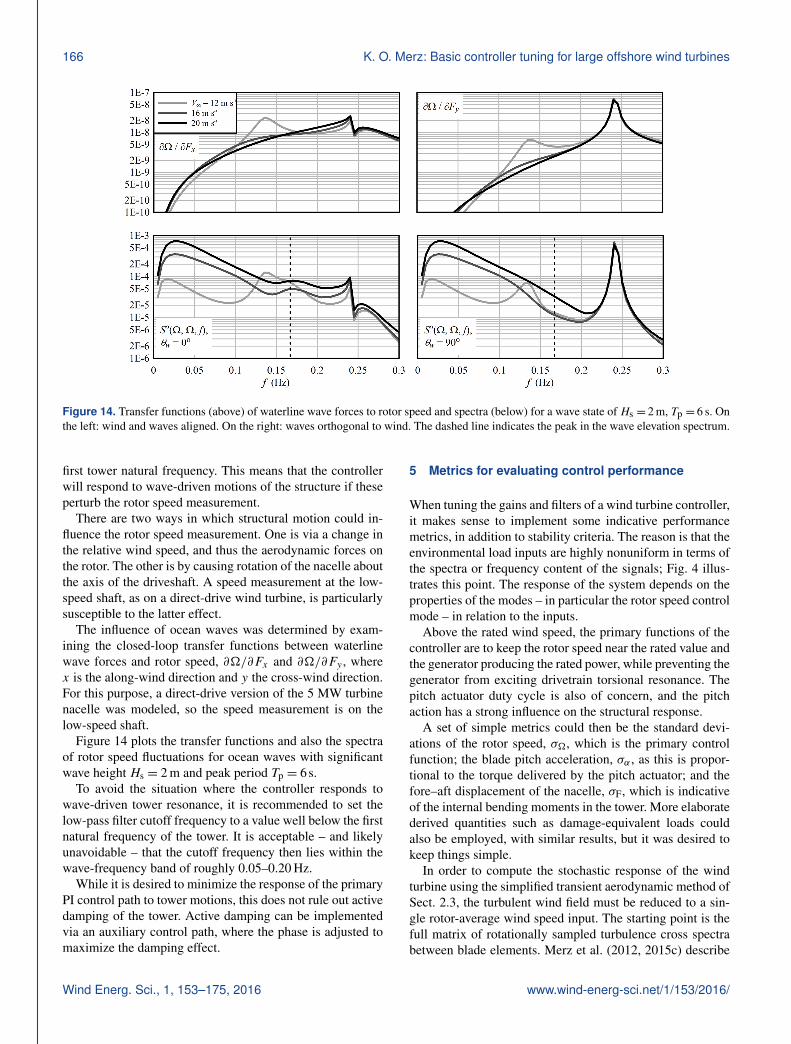
Figure 14. Transfer functions (above) of waterline wave forces to rotor speed and spectra (below) for a wave state of Hs = 2 m, Tp = 6 s. Onthe left: wind and waves aligned. On the right: waves orthogonal to wind. The dashed line indicates the peak in the wave elevation spectrum.

first tower natural frequency. This means that the controllerwill respond to wave-driven motions of the structure if theseperturb the rotor speed measurement.

There are two ways in which structural motion could in-fluence the rotor speed measurement. One is via a change inthe relative wind speed, and thus the aerodynamic forces onthe rotor. The other is by causing rotation of the nacelle aboutthe axis of the driveshaft. A speed measurement at the low-speed shaft, as on a direct-drive wind turbine, is particularlysusceptible to the latter effect.

The influence of ocean waves was determined by exam-ining the closed-loop transfer functions between waterlinewave forces and rotor speed, ∂�/∂Fx and ∂�/∂Fy , wherex is the along-wind direction and y the cross-wind direction.For this purpose, a direct-drive version of the 5 MW turbinenacelle was modeled, so the speed measurement is on thelow-speed shaft.

Figure 14 plots the transfer functions and also the spectraof rotor speed fluctuations for ocean waves with significantwave height Hs = 2 m and peak period Tp = 6s.

To avoid the situation where the controller responds towave-driven tower resonance, it is recommended to set thelow-pass filter cutoff frequency to a value well below the firstnatural frequency of the tower. It is acceptable – and likelyunavoidable – that the cutoff frequency then lies within thewave-frequency band of roughly 0.05–0.20 Hz.

While it is desired to minimize the response of the primaryPI control path to tower motions, this does not rule out activedamping of the tower. Active damping can be implementedvia an auxiliary control path, where the phase is adjusted tomaximize the damping effect.

5 Metrics for evaluating control performance

When tuning the gains and filters of a wind turbine controller,it makes sense to implement some indicative performancemetrics, in addition to stability criteria. The reason is that theenvironmental load inputs are highly nonuniform in terms ofthe spectra or frequency content of the signals; Fig. 4 illus-trates this point. The response of the system depends on theproperties of the modes – in particular the rotor speed controlmode – in relation to the inputs.

Above the rated wind speed, the primary functions of thecontroller are to keep the rotor speed near the rated value andthe generator producing the rated power, while preventing thegenerator from exciting drivetrain torsional resonance. Thepitch actuator duty cycle is also of concern, and the pitchaction has a strong influence on the structural response.

A set of simple metrics could then be the standard devi-ations of the rotor speed, σ�, which is the primary controlfunction; the blade pitch acceleration, σα , as this is propor-tional to the torque delivered by the pitch actuator; and thefore–aft displacement of the nacelle, σF, which is indicativeof the internal bending moments in the tower. More elaboratederived quantities such as damage-equivalent loads couldalso be employed, with similar results, but it was desired tokeep things simple.

In order to compute the stochastic response of the windturbine using the simplified transient aerodynamic method ofSect. 2.3, the turbulent wind field must be reduced to a sin-gle rotor-average wind speed input. The starting point is thefull matrix of rotationally sampled turbulence cross spectrabetween blade elements. Merz et al. (2012, 2015c) describe



the methods used to generate this spectral matrix. Velocitycross spectra between each pair of rotating blade elementsare computed analytically using isotropic turbulence theory,together with the Von Karman spectrum. The resulting spec-tral matrix is transformed into multiblade coordinates, givingthe characteristic 3 nP signals in the ground-fixed frame.

The collective multiblade components of the spectral ma-trix are retained, and the cosine and sine components are dis-carded. Then an averaging procedure is performed, weight-ing the contribution at each blade element according to itsswept area (≈ 2πreLe), which is used as a surrogate forhow important each radial station is to the rotor loading. Theequation for the weighted average is

Su (f )=(Le ◦ re)T Su(f ) (Le ◦ re)(∑

k

Le,z,kre, k

)2 , (13)

where Le and re are column vectors of the spanwise lengthand radial coordinate of each blade element, Su is the spectralmatrix of collective multiblade components of turbulence,and ◦ denotes element-wise multiplication (Hadamard prod-uct).

In cases with ocean waves, the wave force spectrum isderived by running a time-domain hydrodynamic analysis,summing the forces to a point on the tower at the waterlineand computing the spectrum from the time series of forces.

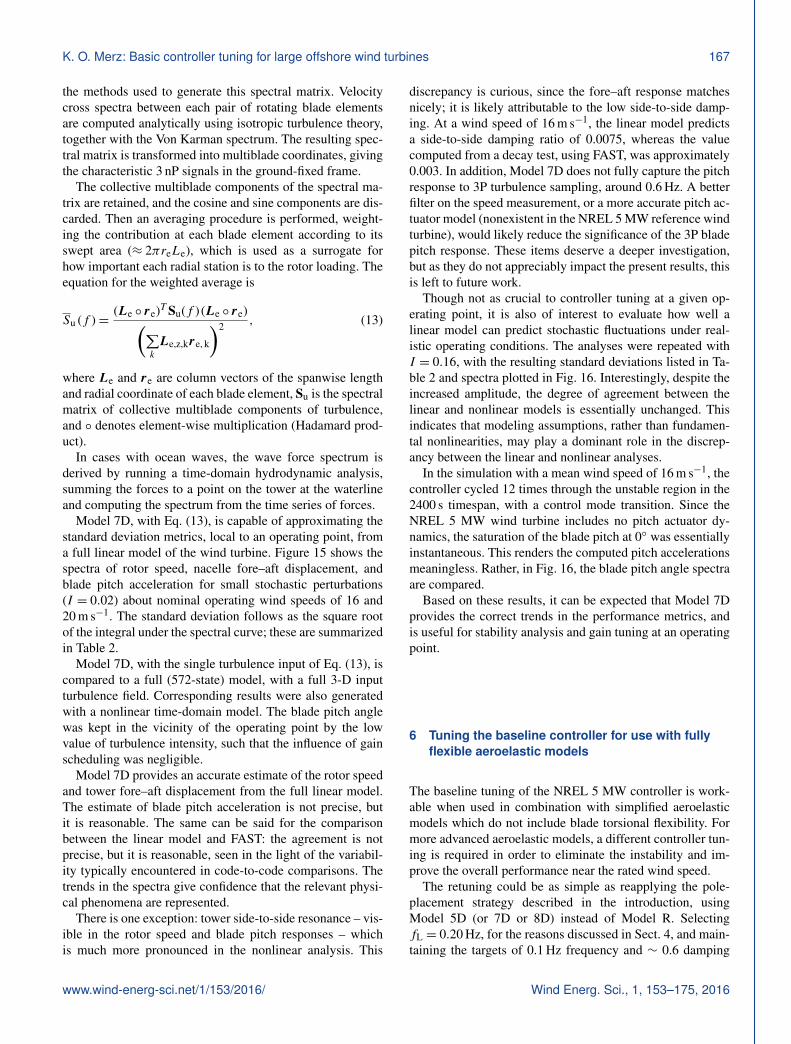
Model 7D, with Eq. (13), is capable of approximating thestandard deviation metrics, local to an operating point, froma full linear model of the wind turbine. Figure 15 shows thespectra of rotor speed, nacelle fore–aft displacement, andblade pitch acceleration for small stochastic perturbations(I = 0.02) about nominal operating wind speeds of 16 and20 m s−1. The standard deviation follows as the square rootof the integral under the spectral curve; these are summarizedin Table 2.

Model 7D, with the single turbulence input of Eq. (13), iscompared to a full (572-state) model, with a full 3-D inputturbulence field. Corresponding results were also generatedwith a nonlinear time-domain model. The blade pitch anglewas kept in the vicinity of the operating point by the lowvalue of turbulence intensity, such that the influence of gainscheduling was negligible.

Model 7D provides an accurate estimate of the rotor speedand tower fore–aft displacement from the full linear model.The estimate of blade pitch acceleration is not precise, butit is reasonable. The same can be said for the comparisonbetween the linear model and FAST: the agreement is notprecise, but it is reasonable, seen in the light of the variabil-ity typically encountered in code-to-code comparisons. Thetrends in the spectra give confidence that the relevant physi-cal phenomena are represented.

There is one exception: tower side-to-side resonance – vis-ible in the rotor speed and blade pitch responses – whichis much more pronounced in the nonlinear analysis. This

discrepancy is curious, since the fore–aft response matchesnicely; it is likely attributable to the low side-to-side damp-ing. At a wind speed of 16 m s−1, the linear model predictsa side-to-side damping ratio of 0.0075, whereas the valuecomputed from a decay test, using FAST, was approximately0.003. In addition, Model 7D does not fully capture the pitchresponse to 3P turbulence sampling, around 0.6 Hz. A betterfilter on the speed measurement, or a more accurate pitch ac-tuator model (nonexistent in the NREL 5 MW reference windturbine), would likely reduce the significance of the 3P bladepitch response. These items deserve a deeper investigation,but as they do not appreciably impact the present results, thisis left to future work.

Though not as crucial to controller tuning at a given op-erating point, it is also of interest to evaluate how well alinear model can predict stochastic fluctuations under real-istic operating conditions. The analyses were repeated withI = 0.16, with the resulting standard deviations listed in Ta-ble 2 and spectra plotted in Fig. 16. Interestingly, despite theincreased amplitude, the degree of agreement between thelinear and nonlinear models is essentially unchanged. Thisindicates that modeling assumptions, rather than fundamen-tal nonlinearities, may play a dominant role in the discrep-ancy between the linear and nonlinear analyses.

In the simulation with a mean wind speed of 16 m s−1, thecontroller cycled 12 times through the unstable region in the2400 s timespan, with a control mode transition. Since theNREL 5 MW wind turbine includes no pitch actuator dy-namics, the saturation of the blade pitch at 0◦ was essentiallyinstantaneous. This renders the computed pitch accelerationsmeaningless. Rather, in Fig. 16, the blade pitch angle spectraare compared.

Based on these results, it can be expected that Model 7Dprovides the correct trends in the performance metrics, andis useful for stability analysis and gain tuning at an operatingpoint.

6 Tuning the baseline controller for use with fullyflexible aeroelastic models

The baseline tuning of the NREL 5 MW controller is work-able when used in combination with simplified aeroelasticmodels which do not include blade torsional flexibility. Formore advanced aeroelastic models, a different controller tun-ing is required in order to eliminate the instability and im-prove the overall performance near the rated wind speed.

The retuning could be as simple as reapplying the pole-placement strategy described in the introduction, usingModel 5D (or 7D or 8D) instead of Model R. SelectingfL = 0.20 Hz, for the reasons discussed in Sect. 4, and main-taining the targets of 0.1 Hz frequency and ∼ 0.6 damping



Figure 15. Spectra of rotor speed, nacelle fore–aft displacement, and blade pitch acceleration in small-amplitude (I = 0.02) turbulence. Thesimplified Model 7D, with only one rotor-average wind speed input, is compared to a full (572-state) linear model and nonlinear time-domainsimulations. On the left: mean wind speed of 16 m s−1; on the right: 20 m s−1. The x axis of the pitch acceleration plots is extended in orderto include 3P rotationally sampled turbulence.

Table 2. Values of the standard deviation metrics, derived from Figs. 15 and 16.

σ� σα σF

I V∞ 7D Linear FAST 7D Linear FAST 7D Linear FAST

0.0216 0.00556 0.00556 0.00610 0.00073 0.00081 0.00092 0.00842 0.00856 0.0075420 0.00727 0.00733 0.00793 0.00080 0.00091 0.00103 0.00879 0.00974 0.00805

0.1616 0.0445 0.0445 0.0480 0.00590 0.00653 n/a 0.0674 0.0684 0.070820 0.0582 0.0586 0.0600 0.00649 0.00736 0.00895 0.0703 0.0779 0.0669

ratio, the gains are then scheduled as

KP = 0.5679− 3.409β + 21.07β2− 67.78β3

+ 74.77β4

KI = 0.05417− 0.5909β + 7.454β2− 24.19β3

+ 26.69β4, (14)

where β has units of radians, KP of s, and KI is dimension-less. The values in Eq. (14) are valid for 0≤ β ≤ 0.40 rad;for transient excursions above 0.40 rad during normal op-eration, the gains are computed according to β = 0.40 rad.A fourth-order polynomial provides a smooth, accurate fitthrough points generated at integer wind speeds between 12

and 25 m s−1, with a refined resolution between 11.4 and12 m s−1.

An alternative, in the manner of Tibaldi et al. (2012), is totune the controller gains and filters based upon an evaluationof system performance. Here we use the metrics of Sect. 5,together with Model 7D. This model runs quickly enoughthat a complete mapping of the tuning parameters, within rea-sonable bounds, is feasible. Sophisticated optimization tech-niques are not needed.



Figure 16. The results of Fig. 16, repeated with I = 0.16. On the left: mean wind speed of 16 m s−1; on the right: 20 m s−1. The figure inthe lower left is the spectrum of blade pitch angle; the spectrum of pitch acceleration is meaningless, due to the abrupt saturation of the pitchangle at 0◦.

Figure 17. Points on the Pareto front, plotted according to the objectives (on the left) and the control tuning parameters (on the right). Thewind speed is 16 m s−1.

As an example of one possible approach for tuning thecontroller, consider the case with a mean wind speed of16 m s−1. For appropriate weighting of wind and wave loads,

a realistic value of the turbulence intensity is selected: theIEC Class IB normal turbulence model gives I = 0.154. Anocean wave climate of Hs = 2 m and Tp = 6s is representa-



Table 3. The pole-placement tuning and resulting metrics. The low-pass filter frequency fL is 0.20 Hz in all cases. For abbreviations, pleasesee the table in Appendix A.

V∞ β0 KP KI σF σS σ� σβ σα σd σf σe

12 0.064 0.420 0.040 0.143 0.052 0.0930 0.069 0.0030 0.0036 1.223 0.04013 0.109 0.370 0.050 0.112 0.052 0.0726 0.053 0.0031 0.0024 0.921 0.02314 0.143 0.350 0.066 0.101 0.052 0.0612 0.048 0.0034 0.0019 0.805 0.02415 0.173 0.330 0.075 0.096 0.052 0.0574 0.045 0.0036 0.0017 0.738 0.02916 0.201 0.310 0.085 0.094 0.051 0.0551 0.044 0.0039 0.0015 0.704 0.03517 0.226 0.280 0.090 0.094 0.052 0.0559 0.043 0.0040 0.0014 0.687 0.04118 0.250 0.260 0.095 0.094 0.052 0.0563 0.043 0.0041 0.0013 0.675 0.04619 0.272 0.240 0.105 0.097 0.052 0.0563 0.043 0.0043 0.0012 0.671 0.05220 0.294 0.220 0.107 0.099 0.053 0.0580 0.043 0.0044 0.0011 0.668 0.05721 0.315 0.205 0.115 0.102 0.053 0.0584 0.043 0.0047 0.0011 0.668 0.06322 0.335 0.188 0.120 0.105 0.054 0.0598 0.043 0.0048 0.0010 0.670 0.06823 0.354 0.174 0.128 0.109 0.054 0.0605 0.044 0.0051 0.0010 0.674 0.07324 0.374 0.160 0.134 0.113 0.055 0.0616 0.044 0.0053 0.0010 0.677 0.07825 0.392 0.146 0.138 0.118 0.056 0.0632 0.044 0.0054 0.0010 0.681 0.083

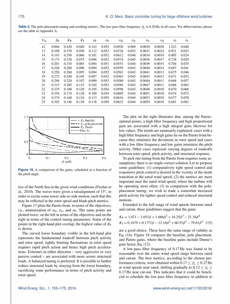
Figure 18. A comparison of the gains, scheduled as a function ofthe pitch angle.

tive of the North Sea in the given wind conditions (Fischer etal., 2010). The waves were given a misalignment of 15◦, inorder to excite some tower side-to-side motion, such that thismay be reflected in the rotor speed and blade pitch metrics.

Figure 17 plots the Pareto front, in terms of the objectives,i.e., minimization of σ�, σα , and σF. The same points areplotted twice: on the left in terms of the objectives and on theright in terms of the control tuning parameters. Some of thepoints in the right-hand plot overlap; the highest value of KIis shown.

The curved lower boundary visible in the left-hand plotrepresents the fundamental tradeoff between pitch activityand rotor speed; tightly limiting fluctuations in rotor speedrequires rapid pitch action and hence high pitch accelera-tions. Extremes in either direction – very aggressive or verypassive control – are associated with more severe structuralloads. A balanced tuning is preferred. It is possible to furtherreduce structural loads by straying from the lower boundary,sacrificing some performance in terms of pitch activity androtor speed.

The plot on the right illustrates that, among the Pareto-optimal points, a high filter frequency and high proportionalgain are associated with a high integral gain; likewise forlow values. The trends are summarily explained: cases with ahigh filter frequency and high gains lie on the Pareto front be-cause they minimize the deviations in rotor speed and caseswith a low filter frequency and low gains minimize the pitchactivity. Other cases represent varying degrees of tradeoffsbetween rotor speed, pitch activity, and structural response.

To pick one tuning from the Pareto front requires some as-sumptions; there is no single correct solution. Let us proposesome guidelines: (1) comparatively tight speed control andresponsive pitch control is desired in the vicinity of the modetransition at the rated wind speed; (2) the metrics are moreimportant near the rated wind speed, where the turbine willbe operating most often; (3) in comparison with the pole-placement tuning, we wish to trade a somewhat increasedpitch activity for tighter speed control and reduced structuralmotions.

Extended to the full range of wind speeds between ratedand cutout, these guidelines suggest that the gains

KP = 1.071− 3.651β + 1.666β2+ 16.25β3

− 21.34β4

KI = 0.1679+ 0.1771β − 12.16β2+ 60.52β3

− 79.61β4 (15)

are a good choice. These have the same range of validity asEq. (14). Figure 18 compares the baseline, pole placement,and Pareto gains, where the baseline gains include Dunne’sgain factor, Eq. (12).

A low-pass filter frequency of 0.17 Hz was found to bereasonable over the entire wind speed range between ratedand cutout. The best metrics, according to the chosen per-formance criteria, were obtained within 0.17≤ fL ≤ 0.27 Hzat wind speeds near rated, shifting gradually to 0.12≤ fL ≤

0.17 Hz near cut-out. This indicates that it could be benefi-cial to schedule the low-pass filter frequency in addition to



Table 4. The selected Pareto tuning and resulting metrics. The low-pass filter frequency fL is 0.17 Hz in all cases. For abbreviations, pleasesee the table in Appendix A.

V∞ β0 KP KI σF σS σ� σβ σα σd σf σe

12 0.064 0.846 0.144 0.135 0.047 0.0347 0.067 0.0057 0.0033 1.185 0.03413 0.109 0.717 0.110 0.104 0.048 0.0361 0.052 0.0054 0.0022 0.865 0.01814 0.143 0.621 0.088 0.093 0.048 0.0402 0.047 0.0052 0.0018 0.742 0.02015 0.173 0.550 0.077 0.089 0.049 0.0438 0.044 0.0052 0.0016 0.676 0.02516 0.201 0.499 0.074 0.087 0.049 0.0461 0.043 0.0052 0.0014 0.643 0.03017 0.226 0.462 0.078 0.087 0.049 0.0468 0.042 0.0054 0.0013 0.624 0.03518 0.250 0.435 0.087 0.089 0.049 0.0466 0.042 0.0057 0.0012 0.616 0.04119 0.272 0.414 0.099 0.092 0.049 0.0461 0.042 0.0060 0.0011 0.613 0.04620 0.294 0.398 0.112 0.095 0.050 0.0457 0.042 0.0065 0.0011 0.613 0.05121 0.315 0.386 0.125 0.099 0.050 0.0454 0.042 0.0070 0.0010 0.615 0.05622 0.335 0.376 0.136 0.104 0.051 0.0455 0.043 0.0075 0.0009 0.617 0.06023 0.354 0.369 0.142 0.109 0.051 0.0461 0.043 0.0080 0.0009 0.618 0.06524 0.374 0.368 0.142 0.114 0.052 0.0467 0.043 0.0086 0.0009 0.615 0.06925 0.392 0.375 0.135 0.119 0.052 0.0477 0.042 0.0092 0.0009 0.610 0.072

Table 5. Modal frequency and damping properties of the pole-placement tuning. For abbreviations, including subscripts, please see the tablein Appendix A.

V∞ fDW ζDW fRSC ζRSC fS ζS fF ζF ff ζf fd ζd

12 0.008 0.905 0.101 0.617 0.242 0.0063 0.249 0.090 0.891 0.682 1.850 0.07813 0.009 0.924 0.101 0.621 0.242 0.0062 0.249 0.093 0.912 0.676 1.849 0.07714 0.009 0.953 0.101 0.617 0.242 0.0062 0.249 0.097 0.911 0.681 1.847 0.07615 0.009 0.967 0.102 0.618 0.242 0.0063 0.248 0.100 0.903 0.693 1.844 0.07516 0.008 0.984 0.102 0.609 0.242 0.0064 0.248 0.102 0.910 0.695 1.840 0.07517 0.005 0.994 0.100 0.624 0.242 0.0065 0.247 0.104 0.917 0.696 1.837 0.07418 0.004 0.996 0.102 0.620 0.242 0.0066 0.246 0.107 0.923 0.697 1.833 0.07319 0.000 > 1 0.100 0.619 0.242 0.0068 0.246 0.109 0.929 0.699 1.829 0.07220 0.000 > 1 0.101 0.628 0.242 0.0070 0.245 0.112 0.934 0.702 1.824 0.07121 0.000 > 1 0.102 0.620 0.242 0.0071 0.244 0.114 0.939 0.704 1.819 0.07022 0.000 > 1 0.101 0.627 0.242 0.0074 0.243 0.116 0.945 0.707 1.815 0.06923 0.000 > 1 0.101 0.618 0.242 0.0076 0.242 0.118 0.952 0.711 1.810 0.06924 0.035 0.984 0.101 0.619 0.242 0.0078 0.241 0.119 0.975 0.725 1.804 0.06825 0.061 0.954 0.100 0.623 0.242 0.0080 0.240 0.120 0.962 0.712 1.799 0.067

the gains. There is no particular difficulty in doing so. Atthe same time, the observed benefits were minor, and it wasdecided that these did not justify diverging from the base-line control strategy of a constant low-pass filter frequency.It is also worth noting that a filter frequency of 0.17 Hz ishigh enough that it does not interfere with energy production(maximum CP tracking) below the rated wind speed.

Tables 3 and 4 list the gains, together with the primarymetrics σ�, σα , and σF, used to generate the Pareto front.Standard deviations of other degrees of freedom are alsoshown. These tables were generated with IEC Class IB nor-mal turbulence and the ocean wave conditions mentionedpreviously. Tables 5 and 6 list the frequency and dampingproperties of selected system modes.

The “preferred” damping ratio of the rotor speed controlmode is roughly 0.3, in contrast with the value of 0.6 cho-

sen for pole placement. Tighter control of the rotor speedis achieved not by increasing the damping but rather by in-creasing the frequency. This moves the peak in the ∂�/∂utransfer function away from the high-energy, low-frequencyturbulence, giving response spectra as shown in Fig. 19. Notethat the magnitude of the pitch angle fluctuations is nearly in-dependent of the tuning; thus, the pitch acceleration dependsprimarily upon the frequency.

There are limits to where the pole of the rotor speed con-trol mode can be placed by varying KP and KI. High levelsof damping are associated with low frequencies, where theenergy in the turbulence is concentrated. There is thereforea tradeoff between the robustness of the controller and thedegree to which the rotor speed responds to turbulence. Forthis reason the gain margin of the selected Pareto-optimumcontroller, with a minimum of 2.24 at a wind speed of



Table 6. Modal frequency and damping properties of the selected Pareto tuning. For abbreviations, including subscripts, please see the tablein Appendix A.

V∞ fDW ζDW fRSC ζRSC fS ζS fF ζF ff ζf fd ζd

12 0.000 > 1 0.129 0.242 0.242 0.0064 0.254 0.101 0.901 0.680 1.836 0.07713 0.000 > 1 0.133 0.268 0.242 0.0064 0.254 0.105 0.919 0.674 1.840 0.07714 0.000 > 1 0.135 0.307 0.242 0.0064 0.252 0.108 0.916 0.680 1.841 0.07615 0.004 0.985 0.136 0.340 0.242 0.0065 0.251 0.111 0.907 0.692 1.840 0.07516 0.003 0.993 0.139 0.356 0.242 0.0066 0.250 0.114 0.913 0.694 1.838 0.07417 0.003 0.993 0.142 0.361 0.242 0.0068 0.249 0.117 0.919 0.695 1.835 0.07418 0.005 0.989 0.145 0.359 0.242 0.0069 0.248 0.122 0.926 0.697 1.831 0.07319 0.006 0.984 0.149 0.353 0.242 0.0071 0.247 0.127 0.931 0.699 1.827 0.07220 0.008 0.982 0.153 0.343 0.242 0.0073 0.246 0.132 0.937 0.701 1.823 0.07121 0.009 0.982 0.158 0.331 0.242 0.0075 0.245 0.139 0.943 0.703 1.818 0.07022 0.009 0.983 0.164 0.319 0.242 0.0077 0.244 0.147 0.949 0.706 1.813 0.06923 0.010 0.999 0.172 0.307 0.242 0.0080 0.242 0.158 0.956 0.710 1.808 0.06924 0.024 0.995 0.184 0.288 0.242 0.0083 0.239 0.176 0.978 0.723 1.803 0.06825 0.030 0.993 0.200 0.245 0.242 0.0087 0.233 0.210 0.966 0.711 1.798 0.067

Figure 19. An example of how tighter speed control is obtained by increasing the frequency of the rotor speed control mode. The wind speedis 16 m s−1.

12.0 m s−1, is lower than would be chosen if the controllerwere designed without knowledge of the turbulence.

The natural frequency of the rotor speed control modetends to increase at wind speeds approaching cutout. Thepole-placement technique, holding the frequency at 0.1 Hz,requires a comparatively high integral gain (Table 3) in re-lation to the proportional gain – the integral path acts as anegative stiffness on the speed fluctuations.

7 Conclusions

There is no single reference control tuning which performswell with all types of wind turbine models. It is therefore in-cumbent upon the analyst to understand the properties andlimitations of the model and select a control tuning that givesthe desired behavior. The aspects of behavior relevant to con-trol tuning can be largely understood in terms of the rotorspeed control mode of the closed-loop system.

Rule-of-thumb methods, using pole placement on a rigidrotor, are inadequate. The NREL 5 MW wind turbine con-troller was tuned in this manner, and it is unstable near therated wind speed when paired with a fully flexible aeroelastic

model. This calls into question some of the comparisons be-tween optimal and PI controllers which have been publishedover the last decade.

Simple models, with 16–20 states, can be used to tune thecontroller for use with a fully flexible aeroelastic model. Thedegrees of freedom must be selected with care: at a min-imum, a model for control tuning requires tower fore–aft,driveshaft, blade-flap-wise, and blade torsional flexibility. Adynamic wake model is also needed.

The control tuning models can be generated in an auto-mated manner from full linearized models, which are com-monly available as output from aeroelastic codes. The matri-ces are partitioned, retaining only the rows and columns asso-ciated with the selected states. It is acceptable, for purposesof control tuning, to retain only one set of transient aero-dynamic equations, which then represents the rotor-averageaerodynamic response. The appropriate representation of theturbulent wind spectrum then becomes a challenge. A simplesolution is to use the swept-area-weighted average of the col-lective, rotationally sampled turbulence components associ-



ated with each blade element. The spectral matrix is therebyreduced to a single scalar input.

The proper architecture of a gain-scheduled PI controllerplaces the scheduled integral gain inside the integral of theerror.

Ocean waves, especially when misaligned with respect tothe wind, drive tower side-to-side vibrations, to which thepitch controller may respond. It is recommended to low-passfilter the shaft speed measurement with a cutoff frequencythat is well below the frequency of the first tower fore–aftmode.

A revised controller tuning was developed for theNREL 5 MW wind turbine, reducing the low-pass filter cut-off frequency and rescheduling the gains. A Pareto optimiza-tion approach was used in order to identify a set of gainswhich give a stable, balanced performance in terms of min-imizing the rotor speed error, the blade pitch accelerations,and the structural motions.

8 Data availability

The data files associated with the figures and tables arearchived by SINTEF Energy Research. Requests for accessto the data may be sent to the corresponding author.



Appendix A: Nomenclature

A state equation matrix θ generic angleA constant σ standard deviationa generic parameter; axial induction factor τ time constantB state equation matrix 9 integrated speed errorb constant 9

′ weighted integrated speed errorC state equation matrix � rotor speedCP power coefficient � filtered rotor speedc constant; chord ω frequency in rad s−1

D output equation matrixD denominator; diameter Subscriptsd Dunne’s gain factor 0 baseline; mean; multiblade collectiveF force a aerodynamicf frequency in Hz c controlHs significant wave height DW dynamic wake modeI turbulence intensity d driveshaftK gain e edgewise; elementL left-hand side state equation matrix F fore–aftL length f flap-wiseM moment I integralN numerator; number of i inducedP power L low-passq generalized coordinate n naturalR outer radius P proportionalr radius q quasi-steadyS spectrum RSC rotor speed control modes Laplace variable r ratedT torque S side-to-sideTp ocean wave peak period s structural; statesu wind speed fluctuation; generic input u wind speed fluctuationV wind speed; velocity x x directionV∞ undisturbed wind speed y y directionv velocity α blade pitch accelerationv̂ intermediate dynamic wake variable β blade pitch anglex states � rotor speedy generic outputα factor on gains; angle-of-attackβ blade pitch angleζ damping ratio



Acknowledgements. This work has been funded byNOWITECH, the Norwegian Research Centre for OffshoreWind Technology (www.sintef.no/projectweb/nowitech).

Many thanks to Fiona Dunne of the University of Colorado,Boulder, for providing a prepublication version of a manuscriptaddressing the gain scheduling issue of Sect. 3. Thanks also toJason Jonkman of NREL for facilitating this exchange.

Edited by: M. MuskulusReviewed by: two anonymous referees

References

Bossanyi, E. A.: The design of closed loop controllers for wind tur-bines, Wind Energy, 3, 149–163, doi:10.1002/we.34, 2000.

Burton, T., Sharpe, D., Jenkins, N., and Bossanyi, E.: Wind EnergyHandbook, Wiley, Chichester, UK, 2001.

Dunne, F., Aho, J., and Pao, L. Y.: Analysis of gain-scheduling im-plementation for the NREL 5-MW turbine blade pitch controller,manuscript accepted for presentation at the American ControlConference, 6–8 July 2016, Boston, MA, USA, 2016.

Fischer, T., de Vries, W., and Schmidt, B.: Upwind Design Basis,EU UpWind Project, 2010.

Hansen, M. H.: Aeroelastic stability analysis of wind turbinesusing an eigenvalue approach, Wind Energy, 7, 133–143,doi:10.1002/we.116, 2004.

Hansen, M. H., Gaunaa, M., and Madsen, H. A.: A Beddoes-Leishman type dynamic stall model in state-space and indicialformulations, Report Risø-R-1354(EN), Risø National Labora-tory, 2004.

Hansen, M. H., Hansen, A., Larsen, T. J., Øye, S., Sørensen, P., andFuglsang, P.: Control design for a pitch-regulated, variable speedwind turbine, Report Risø-R-1500(EN), Risø National Labora-tory, 2005.

Jafarnejadsani, H. and Pieper, J.: Gain-scheduled L1-optimal con-trol of variable-speed–variable-pitch wind turbines, IEEE T.Contr. Sys. T., doi:10.1109/TCST.2014.2320675, 2014.

Jonkman, B. and Jonkman, J.: FAST v8.15.00a-bjj, National Re-newable Energy Laboratory, 2016.

Jonkman, J. and Musial, W.: Offshore Code Comparison Collabora-tion (OC3) for IEA Task 23 Offshore Wind Technology and De-ployment, Report NREL/TP-5000-48191, National RenewableEnergy Laboratory, 2010.

Jonkman, J., Butterfield, S., Musial, W., and Scott, G.: Definitionof a 5-MW reference wind turbine for offshore system develop-ment, Report NREL/TP-500-38060, National Renewable EnergyLaboratory, 2009.

Kundur, P.: Power System Stability and Control, McGraw-Hill,New York, USA, 1994.

Leithead, W. E. and Connor, B.: Control of variable speed windturbines: dynamic models, Int. J. Control, 73, 1173–1188,doi:10.1080/002071700417830, 2000.

Leishman, J. G.: Challenges in modelling the unsteady aero-dynamics of wind turbines, Wind Energy, 5, 85–132,doi:10.1002/we.62, 2002.

Merz, K. O.: Rapid optimization of stall-regulated wind turbineblades using a frequency-domain method: Part 1, loads analysis,Wind Energy, 18, 1703–1723, doi:10.1002/we.1786, 2015a.

Merz, K. O.: A linear state-space model of an offshore wind turbine,implemented in the STAS wind power plant analysis program,Report TR A7474, SINTEF Energy Research, 2015b.

Merz, K. O.: Environmental loads for frequency-domain aeroelasticanalysis of offshore wind turbines, Memo AN 15.12.19, SINTEFEnergy Research, 2015c.

Merz, K. O.: Pitch actuator and generator models for wind turbinecontrol system studies, Memo AN 15.12.35, SINTEF Energy Re-search, 2015d.

Merz, K. O., Muskulus, M., and Moe, G.: A simple frequency-domain method for stress analysis of stall-regulated wind tur-bines, Wind Energy, 15, 773–798, doi:10.1002/we.504, 2012.

Øye, S.: Dynamic stall, simulated as time lag of separation, Pro-ceedings of the fourth IEA symposium on the aerodynamics ofwind turbines, 20–21 November 1990, Rome, Italy, 1990.

Schlipf, D., Schlipf, D. J., and Kühn, M.: Nonlinear model pre-dictive control of wind turbines, Wind Energy, 16, 1107–1129,doi:10.1002/we.1533, 2013.

Snel, H. and Schepers, J. G.: Joint investigation of dynamic infloweffects and implementation of an engineering method, ReportECN-C–094-107, Energy Research Centre of the Netherlands,1995.

Spencer, M. D., Stol, K. A., Unsworth, C. P., Cater, J. E., andNorris, S. E.: Model predictive control of a wind turbine usingshort-term wind field predictions, Wind Energy, 16, 417–434,doi:10.1002/we.1501, 2013.

Sønderby, I. B.: Low-order aeroelastic models of wind turbines forcontroller design, Doctoral Thesis, Department of Wind Energy,Technical University of Denmark, 2013.

Sønderby, I. B. and Hansen, M. H.: Open-loop frequency responseanalysis of a wind turbine using a high-order linear aeroelas-tic model, Wind Energy, 17, 1147–1167, doi:10.1002/we.1624,2014.

Tibaldi, C., Hansen, M. H., and Henriksen, L. C.: Optimal tuningfor a classical wind turbine controller, J. Phys. Conf. Ser., 555,012099, doi:10.1088/1742-6596/555/1/012099, 2012.

Tibaldi, C., Henriksen, L. C., Hansen, M. H., and Bak, C.: Windturbine fatigue damage evaluation based on a linear model and aspectral method, Wind Energy, doi:10.1002/we.1898, 2015.

van Engelen, T. G. and Braam, H.: TURBU Offshore, computer pro-gram for frequency domain analysis of horizontal axis offshorewind turbines, Report ECN-C–04-079, Energy Research Centreof the Netherlands, 2004.

van Engelen, T. G. and van der Tempel, J.: Frequency domain loadcalculation for offshore wind turbines (TURBU Offshore), Re-port ECN-RX–04-127, Energy Research Centre of the Nether-lands, 2004.

Wright, A. D.: Modern control design for flexible wind turbines,Report NREL/TP-500-35816, National Renewable Energy Lab-oratory, 2004.

Yang, Z., Li, Y., and Seem, J. E.: Multi-model predic-tive control for wind turbine operation under meanderingwake of upstream turbines, Control Eng. Pract., 45, 37–45,doi:10.1016/j.conengprac.2015.08.009, 2015.

Zhou, K., Doyle, J. C., and Glover, K.: Robust and Optimal Control,Prentice Hall, Upper Saddle River, NJ, USA, 1996.


www.sintef.no/projectweb/nowitech

http://dx.doi.org/10.1002/we.34


http://dx.doi.org/10.1109/TCST.2014.2320675

http://dx.doi.org/10.1080/002071700417830







http://dx.doi.org/10.1088/1742-6596/555/1/012099


http://dx.doi.org/10.1016/j.conengprac.2015.08.009

Documents

Basic controller tuning for large offshore wind · PDF file154 K. O. Merz: Basic controller tuning for large offshore wind turbines The ﬂexibility and aerodynamic response of a real