Basic Concepts of the R Language - UP · Basic Concepts of the R Language L. Torgo [email protected] Faculdade de Ciências / LIAAD-INESC TEC, LA Universidade do Porto Jan, 2017 Basic

Basic Concepts of the R Language

L. Torgo

[email protected]

Faculdade de Ciências / LIAAD-INESC TEC, LAUniversidade do Porto

Jan, 2017

Basic Interaction

Basic interaction with the R console

The most common form of interaction with R is through thecommand line at the console

User types a commandPresses the ENTER keyR “returns” the answer

It is also possible to store a sequence of commands in a file(typically with the .R extension) and then ask R to execute allcommands in the file

© L.Torgo (FCUP - LIAAD / UP) Basic R Concepts Jan, 2017 2 / 61

Basic Interaction

Basic interaction with the R console (2)

We may also use the console as a simple calculator

1 + 3/5 * 6^2

## [1] 22.6


Basic Interaction


We may also take advantage of the many functions available in R

rnorm(5, mean = 30, sd = 10)

## [1] 28.100 4.092 29.904 10.611 23.599

# function composition examplemean(sample(1:1000, 30))

## [1] 530.3


Basic Interaction


We may produce plots

plot(sample(1:10, 5), sample(1:10, 5),main = "Drawing 5 random points",xlab = "X", ylab = "Y")

●

●

●

●

●

2 4 6 8 10

24

68

Drawing 5 random points

X

Y


Variables and Objects

The notion of Variable

In R, data are stored in variables.A variable is a “place” with a name used to store information

Different types of objects (e.g. numbers, text, data tables, graphs,etc.).

The assignment is the operation that allows us to store an objecton a variableLater we may use the content stored in a variable using its name.


Variables and Objects

Basic data types

R objects may store a diverse type of information.

R basic data types

Numbers: e.g. 5, 6.3, 10.344, -2.3, -7Strings : e.g. "hello", "it is sunny", "my name is Ana"Note: one the of the most frequent errors - confusing names ofvariables with text values (i.e. strings)! hello is the name of avariable, whilst "hello" is a string.Logical values: TRUE, FALSENote: R is case-sensitive!TRUE is a logical value; true is the name of a variable.


Variables and Objects The Assignment Operation

The assignment - 1

The assignment operator “<-” allows to store some content on avariable

vat <- 0.2

The above stores the number 0.2 on a variable named vat

Afterwards we may use the value stored on the variable using itsname

priceVAT <- 240 * (1 + vat)

This new example stores the value 288 (= 240 × (1 + 0.2)) on thevariable priceVAT

We may thus put expressions on the right-side of an assignment



The assignement - 2

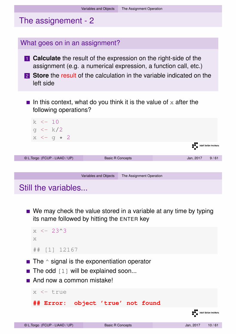
What goes on in an assignment?

1 Calculate the result of the expression on the right-side of theassignment (e.g. a numerical expression, a function call, etc.)

2 Store the result of the calculation in the variable indicated on theleft side

In this context, what do you think it is the value of x after thefollowing operations?

k <- 10g <- k/2x <- g * 2



Still the variables...

We may check the value stored in a variable at any time by typingits name followed by hitting the ENTER key

x <- 23^3x

## [1] 12167

The ^ signal is the exponentiation operatorThe odd [1] will be explained soon...And now a common mistake!

x <- true

## Error: object ’true’ not found



A last note on the assignment operation...

It is important to be aware that the assignment is destructiveIf we assign some content to a variable and this variable wasstoring another content, this latter value is “lost”,

x <- 23x

## [1] 23

x <- 4x

## [1] 4


Functions

Functions

In R almost all operations are carried out by functionsA function is a mathematical notion that maps a set of argumentsinto a result- e.g. the function sin applied to 0.2 gives as result 0.1986693In terms of notation a function has a name and can have 0 ormore arguments that are indicated within parentheses andseparated by commas- e.g. xpto(0.2, 0.3) has the meaning of applying the functionwith the name xpto to the numbers 0.2 and 0.3


Functions

Functions (2)

R uses exactly the same notation for functions.

sin(0.2)

## [1] 0.1987

sqrt(45) # sqrt() calculates the square root

## [1] 6.708


Functions

Creating new functions

Any time we execute a set of operations frequently it may be wise tocreate a new function that runs them automatically.

Suppose we convert two currencies frequently (e.g. Euro-Dollar).We may create a function that given a value in Euros and anexchange rate will return the value in Dollars,

euro2dollar <- function(p, tx) p * txeuro2dollar(3465, 1.36)

## [1] 4712

We may also specify that some of the function parameters havedefault values

euro2dollar <- function(p, tx = 1.34) p * txeuro2dollar(100)

## [1] 134


Functions Function composition

Function Composition

An important mathematical notion is that of function composition- (f ◦ g)(x) = f (g(x)), that means to apply the function f to theresult of applying the function g to xR is a functional language and we will use function compositionextensively as a form of performing several complex operationswithout having to store every intermediate result

x <- 10y <- sin(sqrt(x))y

## [1] -0.02068


Functions Function composition

Function Composition - 2

x <- 10y <- sin(sqrt(x))y

## [1] -0.02068

We could instead do (without function composition):

x <- 10temp <- sqrt(x)y <- sin(temp)y

## [1] -0.02068


Vectors

Vectors

Vectors are a type of R objects that can store sets of values of thesame base type- e.g. the prices of an article sold in several storesEverytime some set of data has something in common and are ofthe same type, it may make sense to store them as a vectorA vector is another example of a content that we may store in a Rvariable


Vectors

Vectors (2)

Let us create a vector with the set of prices of a product across 5different stores

prices <- c(32.4, 35.4, 30.2, 35, 31.99)prices

## [1] 32.40 35.40 30.20 35.00 31.99

Note that on the right side of the assignment we have a call to thefunction c() using as arguments a set of 5 pricesThe function c() creates a vector containing the values receivedas arguments


Vectors

Vectors (3)

The function c() allows us to associate names to the setmembers. In the above example we could associate the name ofthe store with each price,

prices <- c(worten = 32.4, fnac = 35.4, mediaMkt = 30.2,radioPop = 35, pixmania = 31.99)

prices

## worten fnac mediaMkt radioPop pixmania## 32.40 35.40 30.20 35.00 31.99

This makes the vector meaning more clear and will also facilitatethe access to the data as we will see.


Vectors

Vectors (4)

Besides being more clear, theuse of names is alsorecommended as R will takeadvantage of these names inseveral situations.An example is in the creationof graphs with the data:

barplot(prices)worten fnac mediaMkt radioPop pixmania

05

1015

2025

3035


Indexing Basic indexing

Basic Indexing

When we have objects containing several values (e.g. vectors) wemay want to access some of the values individually.That is the main purpose of indexing: access a subset of thevalues stored in a variableIn mathematics we use indices. For instance, x3 usuallyrepresents the 3rd element in a set of values x .In R the idea is similar:

prices <- c(worten=32.4,fnac=35.4,mediaMkt=30.2,radioPop=35,pixmania=31.99)

prices[3]

## mediaMkt## 30.2


Indexing Basic indexing

Basic Indexing (2)

We may also use the vector position names to facilitate indexingprices <- c(worten=32.4,fnac=35.4,

mediaMkt=30.2,radioPop=35,pixmania=31.99)prices["worten"]

## worten## 32.4

Please note that worten appears between quotation marks. Thisis essencial otherwise we would have an error! Why?Because without quotation marks R interprets worten as avariable name and tries to use its value. As it does not exists itcomplains,prices[worten]

## Error: object ’worten’ not found

Read and interpret error messages is one of the key competenceswe should practice.


Indexing Vectors of indices

Vectors of indices

Using vectors as indices we may access more than one vectorposition at the same time

prices <- c(worten=32.4,fnac=35.4,mediaMkt=30.2,radioPop=35,pixmania=31.99)

prices[c(2,4)]

## fnac radioPop## 35.4 35.0

We are thus accessing positions 2 and 4 of vector pricesThe same applies for vectors of names

prices[c("worten", "pixmania")]

## worten pixmania## 32.40 31.99


Indexing Vectors of indices

Vectors of indices (2)

We may also use logical conditions to “query” the data!

prices[prices > 35]

## fnac## 35.4

The idea is that the result of the query are the values in the vectorprices for which the logical condition is trueLogical conditions can be as complex as we want using severallogical operators available in R.What do you think the following instruction produces as result?

prices[prices > mean(prices)]

## fnac radioPop## 35.4 35.0

Please note that this another example of function composition!© L.Torgo (FCUP - LIAAD / UP) Basic R Concepts Jan, 2017 24 / 61

Vectorization

Vectorization of operations

The great majority of R functions and operations can be applied tosets of values (e.g vectors)Suppose we want to know the prices after VAT in our vectorprices

vat <- 0.23(1+vat)*prices


Notice that we have multiplied a number (1.2) by a set of numbers!The result is another set of numbers that are the result of themultiplication of each number by 1.2


Vectorization

Vectorization of operations (2)

Although it does not make a lot of sense, notice this other exampleof vectorization,

sqrt(prices)


By applying the function sqrt() to a vector instead of a singlenumber we get as result a vector with the same size, resultingfrom applying the function to each individual member of the givenvector.


Vectorization

Vectorization of operations (3)

We can do similar things with two sets of numbersSuppose you have the prices of the product on the same stores inanother city,

prices2 <- c(worten=32.5,fnac=34.6,mediaMkt=32,radioPop=34.4,pixmania=32.1)

prices2


What are the average prices on each store over the two cities?

(prices+prices2)/2


Notice how we have summed two vectors!© L.Torgo (FCUP - LIAAD / UP) Basic R Concepts Jan, 2017 27 / 61

Vectorization

Logical conditions involving vectors

Logical conditions involving vectors are another example ofvectorizationprices > 35

## worten fnac mediaMkt radioPop pixmania## FALSE TRUE FALSE FALSE FALSE

prices is a set of 5 numbers. We are comparing these 5numbers with one number (35). As before the result is a vectorwith the results of each comparison. Sometimes the condition istrue, others it is false.Now we can fully understand what is going on on a statement likeprices[prices > 35]. The result of this indexing expressionis to return the positions where the condition is true, i.e. this is avector of Boolean values as you may confirm above.


Vectorization

Hands On 1

A survey was carried out on several countries to find out the averageprice of a certain product, with the following resulting data:

Portugal Spain Italy France Germany Greece UK Finland Belgium Austria10.3 10.6 11.5 12.3 9.9 9.3 11.4 10.9 12.1 9.1

1 What is the adequate data structure to store these values?2 Create a variable with this data, taking full advantage of R facilities

in order to facilitate the access to the information.3 Obtain another vector with the prices after VAT.4 Which countries have prices above 10?5 Which countries have prices above the average?6 Which countries have prices between 10 and 11 euros?7 How would you raise the prices by 10%?8 How would you decrease by 2.5%, the prices of the countries with

price above the average?


Vectorization

Hands On 2

Go to the site http://www.xe.com and create a vector with theinformation you obtain there concerning the exchange rate betweensome currencies. You may use the ones appearing at the openingpage.

1 Create a function with 2 arguments: the first is a value in Eurosand the second the name of other currency. The function shouldreturn the corresponding value in the specified currency.

2 What happens if we make a mistake when specifying the currencyname? Try.

3 Try to apply the function to a vector of values provided in the firstargument.


http://www.xe.com

Matrices Basics

Matrices

As vectors, matrices can be used to store sets of values of thesame base type that are somehow relatedContrary to vectors, matrices “spread” the values over twodimensions: rows and collumnsLet us go back to the prices at the stores in two cities. It wouldmake more sense to store them in a matrix, instead of two vectorsColumns could correspond to stores and rows to cities


Matrices Basics

Matrices (2)

Let us see how to create this matrix

prc <- matrix(c(32.40,35.40,30.20, 35.00, 31.99,32.50, 34.60, 32.00, 34.40, 32.01),

nrow=2,ncol=5,byrow=TRUE)prc

## [,1] [,2] [,3] [,4] [,5]## [1,] 32.4 35.4 30.2 35.0 31.99## [2,] 32.5 34.6 32.0 34.4 32.01

The function matrix() can be used to create matricesWe have at least to provide the values and the number of columnsand rows


Matrices Basics

Matrices (3)

prc <- matrix(c(32.40,35.40,30.20, 35.00, 31.99,32.50, 34.60, 32.00, 34.40, 32.01),

nrow=2,ncol=5,byrow=TRUE)prc

## [,1] [,2] [,3] [,4] [,5]## [1,] 32.4 35.4 30.2 35.0 31.99## [2,] 32.5 34.6 32.0 34.4 32.01

The parameter nrow indicates which is the number of rows whilethe parameter ncol provides the number of columnsThe parameter setting byrow=TRUE indicates that the valuesshould be “spread” by row, instead of the default which is bycolumn


Matrices Matrix indexing

Indexing matrices

As with vectors but this time with two dimensionsprc

## [,1] [,2] [,3] [,4] [,5]## [1,] 32.4 35.4 30.2 35.0 31.99## [2,] 32.5 34.6 32.0 34.4 32.01

prc[2, 4]

## [1] 34.4

We may also access a single column or row,

prc[1, ]

## [1] 32.40 35.40 30.20 35.00 31.99

prc[, 2]

## [1] 35.4 34.6


Matrices Matrix indexing

Giving names to Rows and Columns

We may also give names to the two dimensions of matricescolnames(prc) <- c("worten","fnac","mediaMkt","radioPop","pixmania")rownames(prc) <- c("porto","lisboa")prc

## worten fnac mediaMkt radioPop pixmania## porto 32.4 35.4 30.2 35.0 31.99## lisboa 32.5 34.6 32.0 34.4 32.01

The functions colnames() and rownames() may be used to getor set the names of the respective dimensions of the matrixNames can also be used in indexingprc["lisboa", ]


prc["porto", "pixmania"]

## [1] 31.99


Lists

Lists

Lists are ordered collections of other objects, known as thecomponentsList components do not have to be of the same type or size, whichturn lists into a highly flexible data structure.List can be created as follows:lst <- list(id=12323,name="John Smith",

grades=c(13.2,12.4,5.6))lst

## $id## [1] 12323#### $name## [1] "John Smith"#### $grades## [1] 13.2 12.4 5.6


Lists

Indexing Lists

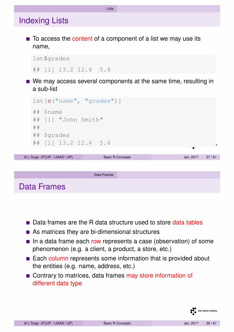
To access the content of a component of a list we may use itsname,

lst$grades

## [1] 13.2 12.4 5.6

We may access several components at the same time, resulting ina sub-list

lst[c("name", "grades")]

## $name## [1] "John Smith"#### $grades## [1] 13.2 12.4 5.6


Data Frames

Data Frames

Data frames are the R data structure used to store data tablesAs matrices they are bi-dimensional structuresIn a data frame each row represents a case (observation) of somephenomenon (e.g. a client, a product, a store, etc.)Each column represents some information that is provided aboutthe entities (e.g. name, address, etc.)Contrary to matrices, data frames may store information ofdifferent data type


Data Frames Creating data frames

Create Data Frames

Usually data sets are already stored in some infrastructureexternal to R (e.g. other software, a data base, a text file, the Web,etc.)Nevertheless, sometimes we may want to introduce the dataourselvesWe can do it in R as followsstud <- data.frame(nrs=c("43534543","32456534"),

names=c("Ana","John"),grades=c(13.4,7.2))

stud

## nrs names grades## 1 43534543 Ana 13.4## 2 32456534 John 7.2


Data Frames Creating data frames

Create Data Frames (2)

If we have too many data tointroduce it is more practical toadd new information using aspreadsheet like editor,

stud <- edit(stud)


Data Frames Indexing data frames

Querying the data

Data frames are visualized as a data table

stud

## nrs names grades## 1 43534543 Ana 13.4## 2 32456534 John 7.2

Data can be accessed in a similar way as in matrices

stud[2,3]

## [1] 7.2

stud[1,"names"]

## [1] Ana## Levels: Ana John



Querying the data (cont.)

Function subset() can be used to easily query the data set

subset(stud,grades > 13,names)

## names## 1 Ana

subset(stud,grades <= 9.5,c(nrs,names))

## nrs names## 2 32456534 John



Hands On Data Frames - Boston Housing

Load in the data set named “Boston” that comes with the packageMASS. This data set describes the median house price in 506 differentregions of Boston. You may load the data doing:data(Boston,package=’MASS’). This should create a data framenamed Boston. You may know more about this data set doinghelp(Boston,package=’MASS’). With respect to this data answerthe following questions:

1 What are the data on the regions with an median price higher than45?

2 What are the values of nox and tax for the regions with anaverage number of rooms (rm) above 8?

3 Which regions have a median price between 10 and 15?4 What is the average criminality rate (crim) for the regions with a

number of rooms above 6?


Data Manipulation with dplyr

The Package dplyr

dplyr is a package that greatly facilitates manipulating data in RIt has several interesting features like:

Implements the most basic data manipulation operationsIs able to handle several data sources (e.g. standard data frames,data bases, etc.)Very fast


Data Manipulation with dplyr Examples of data sources

Data sources

Data frame table (a tibble)A wrapper for a local R data frameMain advantage is printing

library(dplyr)data(iris)ir <- tbl_df(iris)ir

## # A tibble: 150 × 5## Sepal.Length Sepal.Width Petal.Length Petal.Width Species## <dbl> <dbl> <dbl> <dbl> <fctr>## 1 5.1 3.5 1.4 0.2 setosa## 2 4.9 3.0 1.4 0.2 setosa## 3 4.7 3.2 1.3 0.2 setosa## 4 4.6 3.1 1.5 0.2 setosa## 5 5.0 3.6 1.4 0.2 setosa## 6 5.4 3.9 1.7 0.4 setosa## 7 4.6 3.4 1.4 0.3 setosa## 8 5.0 3.4 1.5 0.2 setosa## 9 4.4 2.9 1.4 0.2 setosa## 10 4.9 3.1 1.5 0.1 setosa## # ... with 140 more rows

Similar functions for other data sources (e.g. databases)© L.Torgo (FCUP - LIAAD / UP) Basic R Concepts Jan, 2017 45 / 61

Data Manipulation with dplyr The basic verbs

The basic operations

filter - show only a subset of the rowsselect - show only a subset of the columnsarrange - reorder the rowsmutate - add new columnssummarise - summarise the values of a column



The structure of the basic operations

First argument is a data frame tableRemaining arguments describe what to do with the dataReturn an object of the same type as the first argument (exceptsummarise)Never change the object in the first argument



Filtering rows

filter(data, cond1, cond2, ...) corresponds to the rows ofdata that satisfy ALL indicated conditions.

filter(ir,Sepal.Length > 6,Sepal.Width > 3.5)

## # A tibble: 3 × 5## Sepal.Length Sepal.Width Petal.Length Petal.Width Species## <dbl> <dbl> <dbl> <dbl> <fctr>## 1 7.2 3.6 6.1 2.5 virginica## 2 7.7 3.8 6.7 2.2 virginica## 3 7.9 3.8 6.4 2.0 virginica

filter(ir,Sepal.Length > 7.7 | Sepal.Length < 4.4)

## # A tibble: 2 × 5## Sepal.Length Sepal.Width Petal.Length Petal.Width Species## <dbl> <dbl> <dbl> <dbl> <fctr>## 1 4.3 3.0 1.1 0.1 setosa## 2 7.9 3.8 6.4 2.0 virginica



Ordering rows

arrange(data, col1, col2, ...) re-arranges the rows ofdata by ordering them by col1, then by col2, etc.

arrange(ir,Species,Petal.Width)




Ordering rows - 2

arrange(ir,desc(Sepal.Width),Petal.Length)




Selecting columns

select(data, col1, col2, ...) shows the values of columnscol1, col2, etc. of data

select(ir,Sepal.Length,Species)

## # A tibble: 150 × 2## Sepal.Length Species## <dbl> <fctr>## 1 5.1 setosa## 2 4.9 setosa## 3 4.7 setosa## 4 4.6 setosa## 5 5.0 setosa## 6 5.4 setosa## 7 4.6 setosa## 8 5.0 setosa## 9 4.4 setosa## 10 4.9 setosa## # ... with 140 more rows



Selecting columns - 2

select(ir,-(Sepal.Length:Sepal.Width))

## # A tibble: 150 × 3## Petal.Length Petal.Width Species## <dbl> <dbl> <fctr>## 1 1.4 0.2 setosa## 2 1.4 0.2 setosa## 3 1.3 0.2 setosa## 4 1.5 0.2 setosa## 5 1.4 0.2 setosa## 6 1.7 0.4 setosa## 7 1.4 0.3 setosa## 8 1.5 0.2 setosa## 9 1.4 0.2 setosa## 10 1.5 0.1 setosa## # ... with 140 more rows



Selecting columns - 3

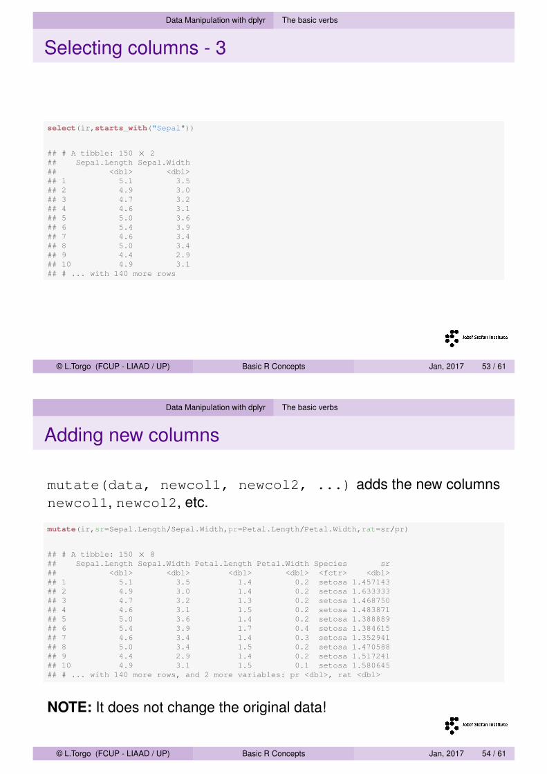
select(ir,starts_with("Sepal"))

## # A tibble: 150 × 2## Sepal.Length Sepal.Width## <dbl> <dbl>## 1 5.1 3.5## 2 4.9 3.0## 3 4.7 3.2## 4 4.6 3.1## 5 5.0 3.6## 6 5.4 3.9## 7 4.6 3.4## 8 5.0 3.4## 9 4.4 2.9## 10 4.9 3.1## # ... with 140 more rows



Adding new columns

mutate(data, newcol1, newcol2, ...) adds the new columnsnewcol1, newcol2, etc.

mutate(ir,sr=Sepal.Length/Sepal.Width,pr=Petal.Length/Petal.Width,rat=sr/pr)

## # A tibble: 150 × 8## Sepal.Length Sepal.Width Petal.Length Petal.Width Species sr## <dbl> <dbl> <dbl> <dbl> <fctr> <dbl>## 1 5.1 3.5 1.4 0.2 setosa 1.457143## 2 4.9 3.0 1.4 0.2 setosa 1.633333## 3 4.7 3.2 1.3 0.2 setosa 1.468750## 4 4.6 3.1 1.5 0.2 setosa 1.483871## 5 5.0 3.6 1.4 0.2 setosa 1.388889## 6 5.4 3.9 1.7 0.4 setosa 1.384615## 7 4.6 3.4 1.4 0.3 setosa 1.352941## 8 5.0 3.4 1.5 0.2 setosa 1.470588## 9 4.4 2.9 1.4 0.2 setosa 1.517241## 10 4.9 3.1 1.5 0.1 setosa 1.580645## # ... with 140 more rows, and 2 more variables: pr <dbl>, rat <dbl>

NOTE: It does not change the original data!


Data Manipulation with dplyr Chaining

Several Operations

select(filter(ir,Petal.Width > 2.3),Sepal.Length,Species)

## # A tibble: 6 × 2## Sepal.Length Species## <dbl> <fctr>## 1 6.3 virginica## 2 7.2 virginica## 3 5.8 virginica## 4 6.3 virginica## 5 6.7 virginica## 6 6.7 virginica



Several Operations (cont.)

Function composition can become hard to understand...

arrange(select(

filter(mutate(ir,sr=Sepal.Length/Sepal.Width),sr > 1.6),

Sepal.Length,Species),Species,desc(Sepal.Length))

## # A tibble: 103 × 2## Sepal.Length Species## <dbl> <fctr>## 1 5.0 setosa## 2 4.9 setosa## 3 4.5 setosa## 4 7.0 versicolor## 5 6.9 versicolor## 6 6.8 versicolor## 7 6.7 versicolor## 8 6.7 versicolor## 9 6.7 versicolor## 10 6.6 versicolor## # ... with 93 more rows



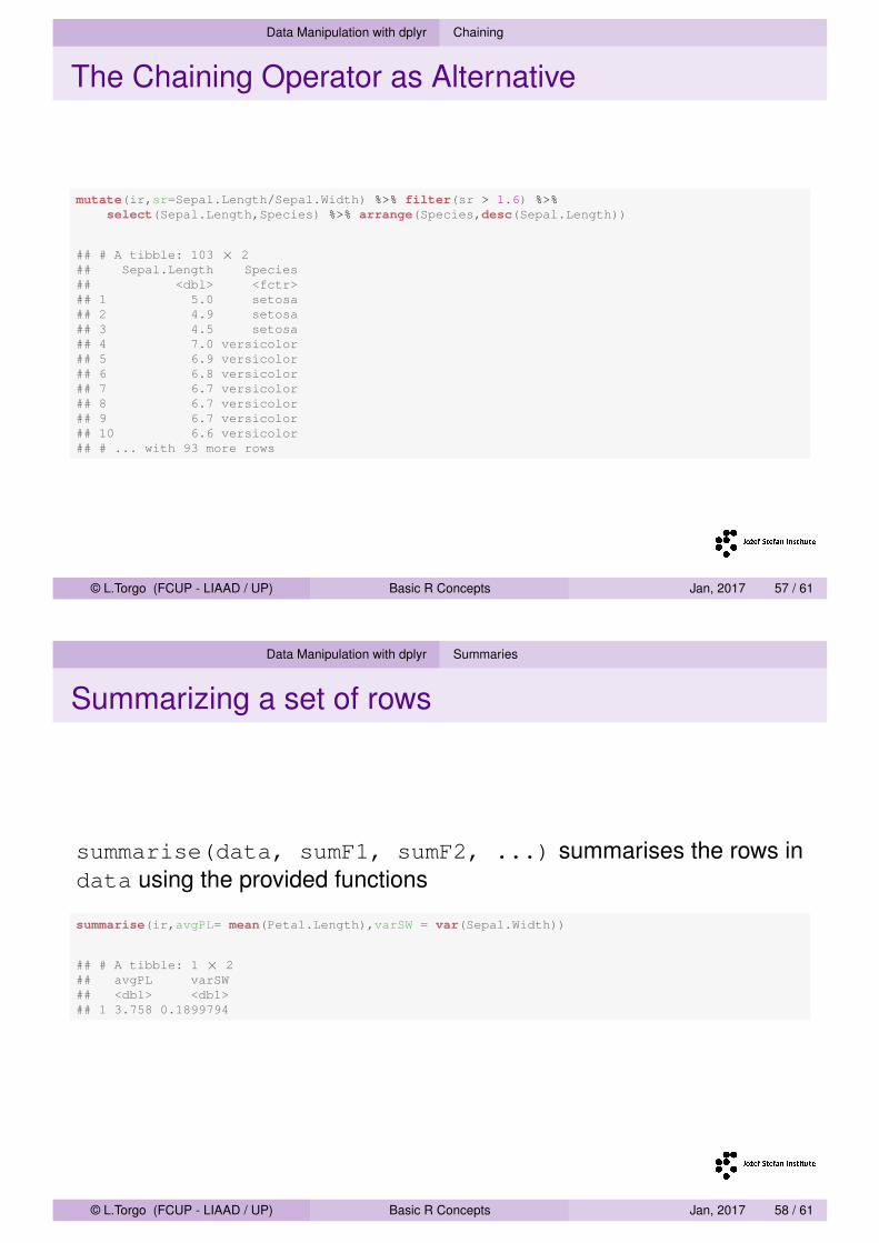
The Chaining Operator as Alternative

mutate(ir,sr=Sepal.Length/Sepal.Width) %>% filter(sr > 1.6) %>%select(Sepal.Length,Species) %>% arrange(Species,desc(Sepal.Length))

## # A tibble: 103 × 2## Sepal.Length Species## <dbl> <fctr>## 1 5.0 setosa## 2 4.9 setosa## 3 4.5 setosa## 4 7.0 versicolor## 5 6.9 versicolor## 6 6.8 versicolor## 7 6.7 versicolor## 8 6.7 versicolor## 9 6.7 versicolor## 10 6.6 versicolor## # ... with 93 more rows


Data Manipulation with dplyr Summaries

Summarizing a set of rows

summarise(data, sumF1, sumF2, ...) summarises the rows indata using the provided functions

summarise(ir,avgPL= mean(Petal.Length),varSW = var(Sepal.Width))

## # A tibble: 1 × 2## avgPL varSW## <dbl> <dbl>## 1 3.758 0.1899794


Data Manipulation with dplyr Groups

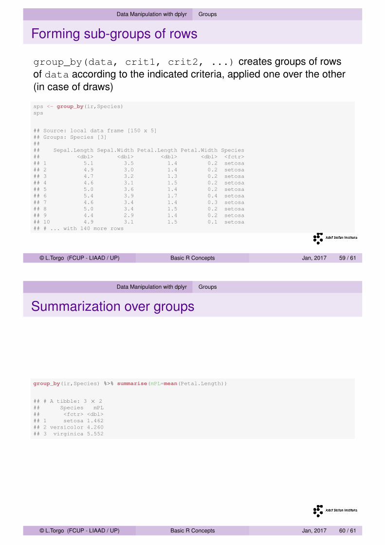
Forming sub-groups of rows

group_by(data, crit1, crit2, ...) creates groups of rowsof data according to the indicated criteria, applied one over the other(in case of draws)

sps <- group_by(ir,Species)sps

## Source: local data frame [150 x 5]## Groups: Species [3]#### Sepal.Length Sepal.Width Petal.Length Petal.Width Species## <dbl> <dbl> <dbl> <dbl> <fctr>## 1 5.1 3.5 1.4 0.2 setosa## 2 4.9 3.0 1.4 0.2 setosa## 3 4.7 3.2 1.3 0.2 setosa## 4 4.6 3.1 1.5 0.2 setosa## 5 5.0 3.6 1.4 0.2 setosa## 6 5.4 3.9 1.7 0.4 setosa## 7 4.6 3.4 1.4 0.3 setosa## 8 5.0 3.4 1.5 0.2 setosa## 9 4.4 2.9 1.4 0.2 setosa## 10 4.9 3.1 1.5 0.1 setosa## # ... with 140 more rows



Summarization over groups

group_by(ir,Species) %>% summarise(mPL=mean(Petal.Length))

## # A tibble: 3 × 2## Species mPL## <fctr> <dbl>## 1 setosa 1.462## 2 versicolor 4.260## 3 virginica 5.552



Hands On Data Manipulation with dplyr

Package mlbench (an extra package that you need to install) containsseveral data sets (from UCI repository). Load the Ozone data set andcheck itis help page to understand what this data is about. Answerthese questions:

1 Create a data frame table with the data for easier manipulation2 What is the average Humidity per Month?3 Show the information of Mondays4 For each combination of Month and Day of the Week obtain the

maximum and minimum temperature at the two locations


Documents

Basic Concepts of the R Language - UP · Basic Concepts of the R Language L. Torgo [email protected] Faculdade de Ciências / LIAAD-INESC TEC, LA Universidade do Porto Jan, 2017 Basic