Embed Size (px)
Citation preview

Basic concepts of microeconomicsand industrial organization:
Consumer and producer behaviourGiovanni Marin
Department of Economics, Society, Politics
Università degli Studi di Urbino ‘Carlo Bo’

Utility function
• Utility can be defined as the satisfaction a consumer derives from the consumption of commodities
• Utility is an ‘ordinal’ concept
– U(2 beers)>U(1 beer)
– Is the U(2 beers) = 2 x U(1 beer)? 3x? 10x? Cardinal differences cannot be measured
Spring 2018 Global Political Economy 2

Utility function
• ‘Well behaved’ utility functions:
– Utility is increasing in consumption
– Utility is increasing at a decreasing rate marginal utility of consumption is decreasing
Spring 2018 Global Political Economy 3

Spring 2018 Global Political Economy 4
x
U(x) Utility function

Spring 2018 Global Political Economy 5
x
U’(x)
Marginal utility function

Utility function with two goods
• We derive utility from the consumption of a bundle of goods
• Assume we can consume two goods: x1 and x2
• U=U(x1,x2)
➢dU/dx1>0; ddU/ddx1<0
➢dU/dx2>0; ddU/ddx2<0
Spring 2018 Global Political Economy 6
Spring 2018 Global Political Economy 7
x1
U(x1, x2)
U(x1, x2=B>A)
U(x1, x2=A)
Indifference curves
Spring 2018 Global Political Economy 8
x1
x2
U’
U’’
U’’>U’
Marginal rate of utility substitution
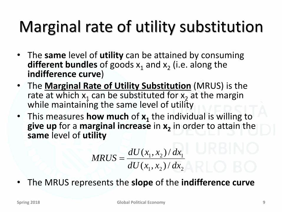
• The same level of utility can be attained by consumingdifferent bundles of goods x1 and x2 (i.e. along the indifference curve)
• The Marginal Rate of Utility Substitution (MRUS) is the rate at which x1 can be substituted for x2 at the marginwhile maintaining the same level of utility
• This measures how much of x1 the individual is willing togive up for a marginal increase in x2 in order to attain the same level of utility
• The MRUS represents the slope of the indifference curve
Spring 2018 Global Political Economy 9
221
121
/),(
/),(
dxxxdU
dxxxdUMRUS
Equilibrium of the consumer
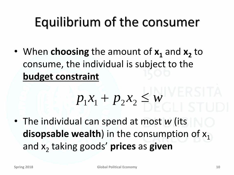
• When choosing the amount of x1 and x2 toconsume, the individual is subject to the budget constraint
• The individual can spend at most w (itsdisopsable wealth) in the consumption of x1
and x2 taking goods’ prices as given
Spring 2018 Global Political Economy 10
wxpxp 2211

Utility maximization
• The individual maximizes its utility subject to the budget constraint:
• Utility is maximized when the marginal rate of utility substitution isequal to the ratio between prices
• Rationale the rate at which the individual is willing to renounceto a marginal amount of good x1 in exchange of a marginal increasein the consumption of good x2 is equal to the relative price of goodx2 in with respect to good x1
Spring 2018 Global Political Economy 11
wxpxp
ts
xxfxxUxx
2211
2121},{
..
),(),( max21
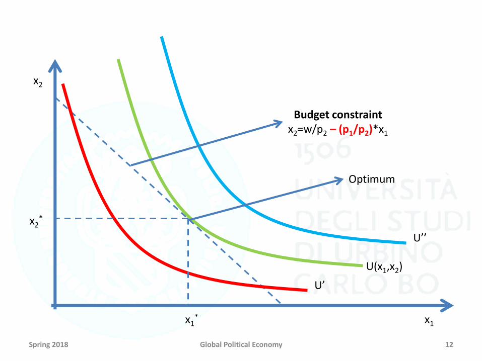
Spring 2018 Global Political Economy 12
x1
x2
U(x1,x2)
U’
U’’
Budget constraintx2=w/p2 – (p1/p2)*x1
x1*
x2*
Optimum

From utility to demand function
Spring 2018 Global Political Economy 13x1
x2
U(x1,x2)
U’

Production with a single input
• Technology describes how the input X (in quantity) is transformed into the output Y (in quantity)
– Total product (production function) Y=Y(X)
• Marginal product
– It is the increase in output Y that is produced by a marginal increase in input X
MP=dY(X)/dX
Spring 2018 Global Political Economy 14
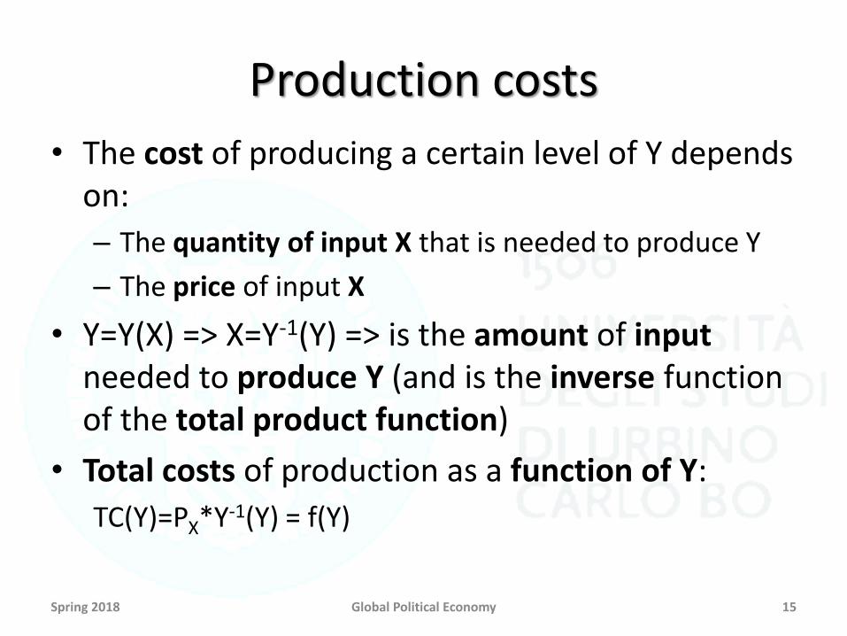
Production costs
• The cost of producing a certain level of Y dependson:
– The quantity of input X that is needed to produce Y
– The price of input X
• Y=Y(X) => X=Y-1(Y) => is the amount of input needed to produce Y (and is the inverse functionof the total product function)
• Total costs of production as a function of Y:
TC(Y)=PX*Y-1(Y) = f(Y)
Spring 2018 Global Political Economy 15

Average and marginal costs
• Average costs are defined as the unitary costof producing a certain output Y
AC(Y)=TC(Y)/Y
• Marginal costs are defined as the cost ofproducing an additional unit of Y
MC(Y)=dTC(Y)/Y
Spring 2018 Global Political Economy 16

Total cost
Spring 2018 Global Political Economy 17
Y
TC(Y)Decreasingmarginalproduct
Increasingmarginalproduct
Constantmarginalproduct

Marginal costs
Spring 2018 Global Political Economy 18
Y
MC(Y) Decreasingmarginalproduct
Increasingmarginalproduct
Constantmarginalproduct

Costs and marginal product
• Decreasing marginal products => convex total costs => increasing marginal costs
• Constant marginal product => linear total costs => constant marginal costs
• Increasing marginal product => concave total costs => decreasing marginal costs
Spring 2018 Global Political Economy 19

Production with two inputs
• Assume that production of Y requires twodifferent inputs– Labour (L)
– Capital (K)
• Production function– Y=Y(K,L)
– A sort of recipe => a certain combination of K and L generates a certain amount of Y
– The production function describes the production technology
Spring 2018 Global Political Economy 20
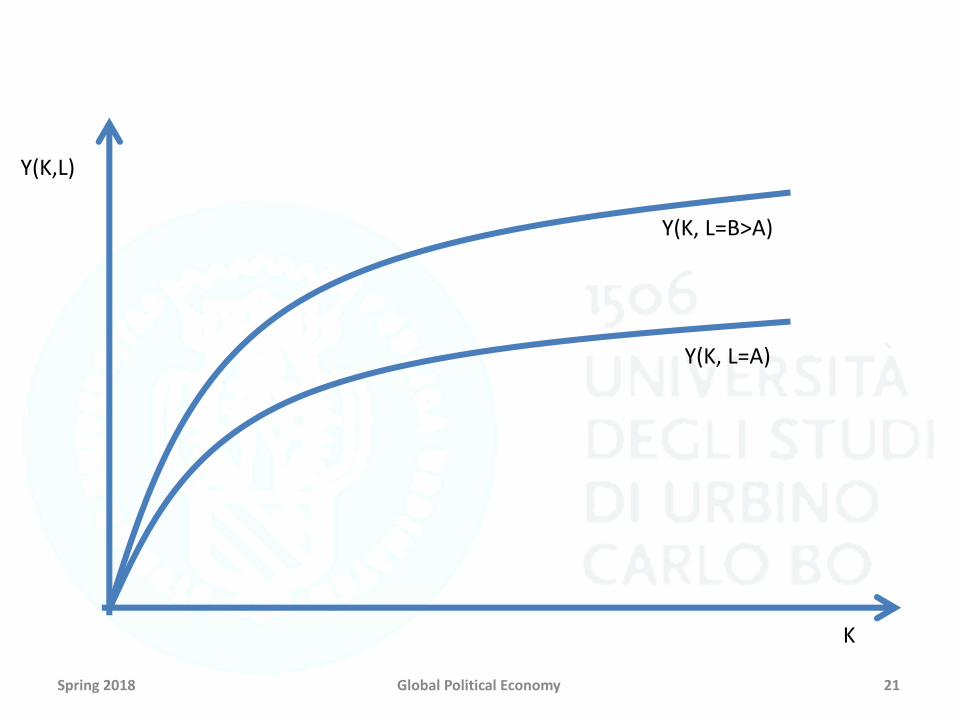
Spring 2018 Global Political Economy 21
K
Y(K,L)
Y(K, L=B>A)
Y(K, L=A)

Isoquants
Spring 2018 Global Political Economy 22
K
L
Y’
Y’’
Y’’>Y’

Marginal rate of technical substitution
• The same level of output can be produced by usingdifferent bundles of inputs L and K (i.e. along the isoquant)
• The Marginal Rate of Technical Substitution (MRTS) is the rate at which L can be substituted for K at the margin whilemaintaining the same level of production
• This measures how much of K the firm can reduce for a marginal increase in L in order to obtain the same level ofproduction
• The MRTS represents the slope of the isoquant
Spring 2018 Global Political Economy 23
dLLKdY
dKLKdYMRTS
/),(
/),(

Properties of the production function
• The production function is strictly increasingin the level of inputs => dY/dL>0; dY/dK>0
• Constant returns to scale => Y(2K,2L)=2*Y(K,L)
• Marginal production of inputs is decreasing
– For a given level of L, a marginal increase in K alsoincreases output, but at an ever decreasing rate (same for K and L) => ddY/ddK<0; ddY/ddL<0
Spring 2018 Global Political Economy 24
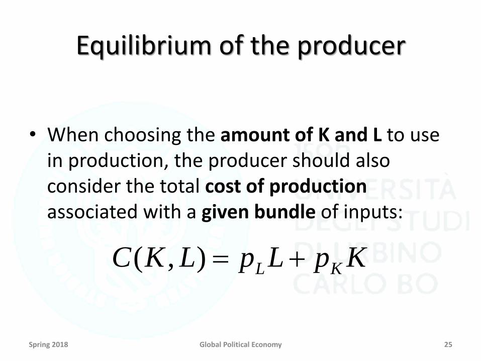
Equilibrium of the producer
• When choosing the amount of K and L to usein production, the producer should alsoconsider the total cost of production associated with a given bundle of inputs:
Spring 2018 Global Political Economy 25
KpLpLKC KL ),(

Cost minimization
• The firm minimize its costs provided the (monetary) output remains at a certain level (isoquant)
• Costs are minimized when the marginal rate of technicalsubstitution is equal to the ratio between prices of inputs
• Rationale the value of marginal product (i.e. price times the marginal quantity produced with a small increase in one input giventhe other input) of each input should equal the price of that input
Spring 2018 Global Political Economy 26
YpLKYp
ts
KpLpLKC
YY
KLK
),(
..
),( minL},{

Spring 2018 Global Political Economy 27
K
L
Y(K,L)
Y’
Y’’
IsocostL=C/pL – (pK/pL)*K
K*
L*
Optimum

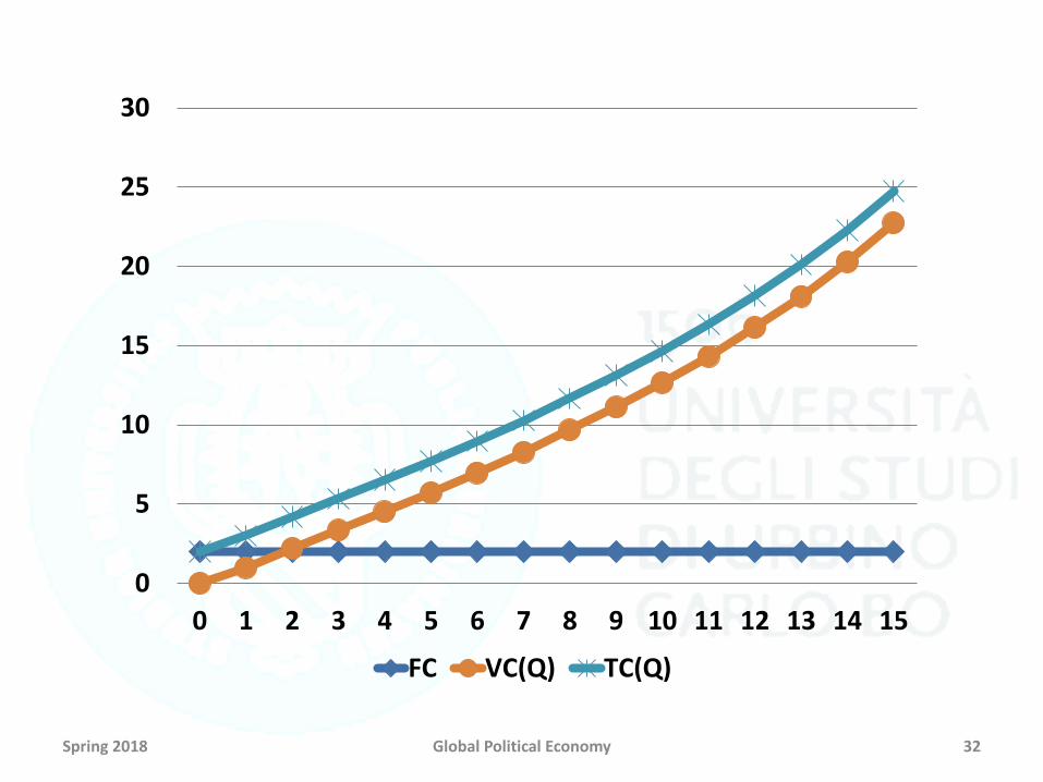
Structure of production costs
• Fixed costs (FC)– They do not vary with the quantity of output that is
produced– The producer will incur fixed costs even with no
production– Average fixed costs per unity of output decrease as output
grows FC/Q
• Variable costs (VC)– Variable costs are function of the quantity of output
produced VC(Q)– As output grows, total variable costs grow– VC(Q=0)=0
Spring 2018 Global Political Economy 28

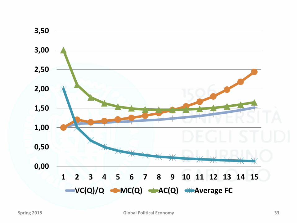
Structure of production costs
• Marginal costs (MC)– Marginal costs represent the change in total costs when output
changes marginally• Fixed costs are constant• Variable costs depend on Q
dTC/dQ=dFC/dQ+dVC(Q)/dQ=0+dVC(Q)/dQ
– They are (usually) function of output MC(Q)
• Average costs (AC)– Average costs represent the average total cost of producing a
certain quantity Q
AC(Q)=FC/Q+VC(Q)/Q
Spring 2018 Global Political Economy 29

Q FC VC(Q)/Q VC(Q) MC(Q) AC(Q) TC(Q)Average
FC
0 2 0 0 - - 2 -
1 2 1.00 1.00 1.00 3.00 3.00 2.00
2 2 1.10 2.20 1.20 2.10 4.20 1.00
3 2 1.11 3.34 1.14 1.78 5.34 0.67
4 2 1.13 4.51 1.17 1.63 6.51 0.50
5 2 1.14 5.72 1.21 1.54 7.72 0.40
6 2 1.16 6.97 1.25 1.50 8.97 0.33
7 2 1.18 8.28 1.31 1.47 10.28 0.29
8 2 1.21 9.66 1.38 1.46 11.66 0.25
9 2 1.23 11.11 1.46 1.46 13.11 0.22
10 2 1.27 12.66 1.55 1.47 14.66 0.20
11 2 1.30 14.33 1.67 1.48 16.33 0.18
12 2 1.34 16.13 1.81 1.51 18.13 0.17
13 2 1.39 18.11 1.98 1.55 20.11 0.15
14 2 1.45 20.30 2.18 1.59 22.30 0.14
15 2 1.52 22.74 2.44 1.65 24.74 0.13
Spring 2018 Global Political Economy 30

Q FC VC(Q)/Q VC(Q) MC(Q) AC(Q) TC(Q)Average
FC
0 2 0 0 - - 2 -
1 2 1.00 1.00 1.00 3.00 3.00 2.00
2 2 1.10 2.20 1.20 2.10 4.20 1.00
3 2 1.11 3.34 1.14 1.78 5.34 0.67
4 2 1.13 4.51 1.17 1.63 6.51 0.50
5 2 1.14 5.72 1.21 1.54 7.72 0.40
6 2 1.16 6.97 1.25 1.50 8.97 0.33
7 2 1.18 8.28 1.31 1.47 10.28 0.29
8 2 1.21 9.66 1.38 1.46 11.66 0.25
9 2 1.23 11.11 1.46 1.46 13.11 0.22
10 2 1.27 12.66 1.55 1.47 14.66 0.20
11 2 1.30 14.33 1.67 1.48 16.33 0.18
12 2 1.34 16.13 1.81 1.51 18.13 0.17
13 2 1.39 18.11 1.98 1.55 20.11 0.15
14 2 1.45 20.30 2.18 1.59 22.30 0.14
15 2 1.52 22.74 2.44 1.65 24.74 0.13
Spring 2018 Global Political Economy 31
MC(Q)=TC(Q)-TC(Q-1)==VC(Q)-VC(Q-1)
Spring 2018 Global Political Economy 32
0
5
10
15
20
25
30
0 1 2 3 4 5 6 7 8 9 10 11 12 13 14 15
FC VC(Q) TC(Q)
Spring 2018 Global Political Economy 33
0,00
0,50
1,00
1,50
2,00
2,50
3,00
3,50
1 2 3 4 5 6 7 8 9 10 11 12 13 14 15
VC(Q)/Q MC(Q) AC(Q) Average FC

Short run vs long run
• In the short run some inputs are fixed– A factory cannot be phased out easily– In the very short run even labour could be fixed
(notice period for firing workers)– Other inputs are variable even in the very short run
(e.g. you can decide to fill the tank of your truck at anytime)
• In the long run all inputs are variable– Factories can be built or dismantled– Workers can be hired or fired– …
Spring 2018 Global Political Economy 34

Stay or exit? Short vs long run
Spring 2018 Global Political Economy 35
Q
P1
AC(Q)
MC(Q)
$
P2
P3

Marginal costs and supply function
• Marginal cost are equivalent, ultimately, to the supply curve– In the short run, the producer is willing to accept any
price greater or equal to the marginal cost to produce a certain quantity Q
– Even if prices are below average costs and thus the company will experience a negative profit due to toohigh fixed costs, it will produce Q anyways to cover asmuch fixed costs as possible
– Marginal profits (P-MC(Q)) are positive as long asP>MC(Q)
Spring 2018 Global Political Economy 36
Market structure
• The market structure how prices and quantityare set on the market
• The market structure depends on (among otherthings):– The number of consumers and producers– The bargaining power of each producer and
consumers
• These factors ultimately depend on:– Cost structure– Shape of demand– Institutional setting (e.g. strength of the antitrust)
Spring 2018 Global Political Economy 37

Market structures
• Perfect competition– Large number of (atomistic) consumers and producers– Each consumer and producer is price taker (i.e. has no
direct influence on prices)
• Monopoly– One single producer and multiple consumers– Consumers are price takers, the producer is price
maker
• Monopsony– One single consumer and multiple producers– The consumer is price maker
Spring 2018 Global Political Economy 38

Market structures
• Oligopoly– Few producers and multiple consumers– Consumers are price takers– Producers have some influence on prices, that also
depends on the behaviour of other producers
• Monopolistic competition– Many consumers with preferences over variety of
goods (that are substitute)– Each producer is the monopolist for the production of
a certain variety– Varieties compete on the market
Spring 2018 Global Political Economy 39

Perfect competition
• Many firms
• Identical and homegenous product
• Each firm is a small part of the market
• Each firm in the market takes the market price asbeing predetermined firms are price takers
• Firms only decide how much to produce for a given price
• Each firm faces a ‘flat’ demand curve
Spring 2018 Global Political Economy 40

Firm
Spring 2018 Global Political Economy 41
Q
MC(Q)
P
Q*

Market
Spring 2018 Global Political Economy 42
Q
Supply=
sum of MC
P
Q*market
=Sum of Q*
Marketdemand

Entry and exit in perfect competition
• In the short run, firms will produce as long asmarginal costs are below the market price (evenif average costs are larger than market prices)
• New firms will enter the market if their expectedmarginal cost is below the prevailing market price
• In the long run, firms with average costs largerthan the market price will exit the market
Spring 2018 Global Political Economy 43

Monopoly
• Only one producer is on the market
• This happens for a number of reasons that generate barrier to entry for potential competitors:– High fixed or sunk costs prevent potential entrants from
entry => natural monopoly• Building a railway infrastructure
• Building an electricity transmission network
– Strategic behaviour of the incumbent that deter entry• Predatory prices
• Large expenditure in advertising
– Government regulation• Gambling and casino (in Italy)
Spring 2018 Global Political Economy 44

Monopoly
• Differently from firms in perfectlycompetitive markets, the monopolist faces a downward sloping demand function
• The monopolist is not price-taker
• The price is set by the monopolist
Spring 2018 Global Political Economy 45

Profit maximization in monopoly
• The monopolist will maximize the followingprofit function:
• Where Q*P(Q) are total revenues and C(Q) are total costs
• Recall that revenues in perfectly competitive markets were Q*P and not Q*P(Q)
Spring 2018 Global Political Economy 46
)()(* max{Q}
QCQPQ

Profit maximization in monopoly
• Profits are maximized when:
• where:
Spring 2018 Global Political Economy 47
dQQdCQMC /)()(
dQQdPQPdQQPQdQMR /)()(/)](*[)(
)()( QMCQMR

Spring 2018 Global Political Economy 48
Q
P
MC
DemandP(Q)
Marginal revenueMR(Q)
QMonopoly QPerf comp
PMonopoly
PPerf comp

Profit function=Q*P(Q)-C(Q)
Spring 2018 Global Political Economy 49
QQMonopoly QPerf comp
Profit

Oligopoly
• Few firms operate on the market
• Firms interact strategically to maximize theirprofits
• A firm decides either prices or quantities, taking into account the behaviour of otherfirms optimal response function
Spring 2018 Global Political Economy 50

Competition on prices (Bertrand)
• Two firms on the market with the samemarginal cost function and no fixed costs
• Firms decide the price
• The firm that sets the lowest price on the market will serve the whole market
• Firms choose their price ‘given’ the price set by other firms
• Firms choose prices simultaneously
Spring 2018 Global Political Economy 51
Competition on prices (Bertrand)
• Firm 1 maximizes profits
• Profits of firm 1 will be➢0 if P1>P2
➢P1*Q(P1)/2-C(Q/2) if P1=P2 the two firms splitequally the market
➢P1*Q(P1)-C(Q) if P1<P2 firm 1 becomes the monopoly
• Firm 2 does the same
• As long as P1*Q(P1)-C(Q)>0 (positive profits), firm1 will set P1<P2
Spring 2018 Global Political Economy 52

Competition on prices (Bertrand)
• In the end, firms will choose a price such thatprofits of each firm are zero MC1=MC2=P1=P2
• No firm has incentive to deviate
– Increasing the price leads to null production
– Reducing the price leads to negative profits
• Same result as in perfect competition!
Spring 2018 Global Political Economy 53

Competition on quantity (Cournot)
• Each firm will set its level of production giventhe expected production of the other firm(s)
• All firms decide their quantity simultaneously
• Firms maximize their profits for givenquantities produced by other firms
Spring 2018 Global Political Economy 54

Competition on quantity (Cournot)
• Assume that two firms operate in the market• Firm 1 maximizes its profits given the expected output
produced by firm 2
• Firm 2 will do the same• The optimal solution for firm 1 is a decreasing function
of the expected quantity produced by firm 2• The larger the quantity produced by firm 2, the lower
the ‘residual demand’ for firm 1 (or alternatively, the lower the expected price)
Spring 2018 Global Political Economy 55
)()Q(Q max 1211}{Q1
QCQP e

Optimal response functions
Spring 2018 Global Political Economy 56
Q2
Q1
)(Q 12
eQf
)(Q 21
eQg
Q*1
Q*2

Oligopoly and collusion
• The Cournot model results in– Prices higher than in perfect competition (and Bertrand
oligopoly) and lower than in monopoly– Quantity lower than in perfect competition (and Bertrand
oligopoly) and higher than in monopoly
• Firms could potentially increase their profits (i.e. total profits earned by producers) by producing the samequantity as the monopolist at the monopoly price collusion
• Firms have great incentive to deviate from collusionas, at the margin, they will earn additional profits fromdeviating
Spring 2018 Global Political Economy 57