Embed Size (px)
Citation preview
The 3rd International Electronic Conference on Geosciences, 7 - 13 December 2020
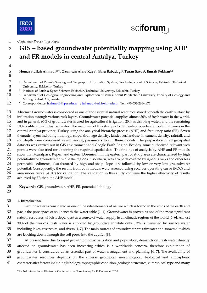
Conference Proceedings Paper 1
GIS – based groundwater potentiality mapping using AHP 2
and FR models in central Antalya, Turkey 3
4
Hemayatullah Ahmadi1,3*, Ozumcan Alara Kaya1, Ebru Babadagi1, Turan Savas2, Emrah Pekkan1,2 5 6
1 Department of Remote Sensing and Geographic Information System, Graduate School of Sciences, Eskisehir Technical 7 University, Eskisehir, Turkey 8
2 Institute of Earth & Space Sciences Eskisehir, Technical University, Eskisehir, Turkey 9 3 Department of Geological Engineering and Exploration of Mines, Kabul Polytechnic University, Faculty of Geology and 10
Mining, Kabul, Afghanistan 11 * Correspondence: [email protected] / [email protected] ; Tel.: +90-552-266-4876 12
Abstract: Groundwater is considered as one of the essential natural resources stored beneath the earth surface by 13 infiltration through various rock layers. Groundwater potential supplies almost 30% of fresh water in the world, 14 and in general, 65% of groundwater is used for agricultural irrigation, 25% as drinking water, and the remaining 15 10% is utilized as industrial water. The main aim of this study is to delineate groundwater potential zones in the 16 central Antalya province, Turkey using the analytical hierarchy process (AHP) and frequency ratio (FR). Seven 17 thematic layers including lithology, slope, drainage density, landcover/landuse, lineament density, rainfall, and 18 soil depth were considered as influencing parameters to run these models. The preparation of all geospatial 19 datasets was carried out in GIS environment and Google Earth Engine. Besides, some authorized relevant web 20 portals were also tried for obtaining the required spatial data. The findings of analysis by AHP and FR models 21 show that Muratpasa, Kepez, and eastern Dosemealti in the eastern part of study area are characterized by high 22 potentiality of groundwater, while the regions in southern, western parts covered by igneous rocks and other less 23 permeable sediments, also featured by high and steep slopes are followed by low or very low groundwater 24 potential. Consequently, the results from both models were assessed using receiver operating curve (ROC) and 25 area under curve (AUC) for validation. The validation in this study confirms the higher effectivity of results 26 achieved by FR than the AHP model. 27
Keywords: GIS, groundwater, AHP, FR, potential, lithology 28 29
1. Introduction 30
Groundwater is considered as one of the vital elements of nature which is found in the voids of the earth and 31
packs the pore space of soil beneath the water table [1–4]. Groundwater is proven as one of the most significant 32
natural resources which is dependent as a source of water supply in all climatic regions of the world [5, 6]. Almost 33
30% of the world’s fresh water is supplied by groundwater while only 0.3% is furnished by surface water 34
including lakes, reservoirs, and rivers [4, 7]. The main sources of groundwater are rainwater and snowmelt which 35
are leaching down through the soil pores into the aquifer [8]. 36
At present time due to rapid growth of industrialization and population, demands on fresh water directly 37
affected on groundwater has been increasing which is a worldwide concern, therefore exploitation of 38
groundwater is considered as an essential part of water management and planning [4, 7]. The availability of 39
groundwater resources depends on the diverse geological, morphological, biological and atmospheric 40
characteristics factors including lithology, topographic condition, geologic structures, climate, soil type and many 41
The 3rd International Electronic Conference on Geosciences, 7 - 13 December 2020
The 3rd International Electronic Conference on Geosciences, 7 - 13 December 2020
other, and the movement mainly depends on the porosity, permeability, transmissibility, and the storage capacity 42
of the rocks [9–12]. 43
There are several approaches for targeting groundwater potential by considering these factors. The 44
applicable methods are geological, geophysical and remote sensing which have been examined by many 45
scientists. The efficiency of methods are varied, some of them are more effective, accurate, time saving and with 46
less cost, while the traditional methods are time consuming and require high expenses [13–15]. Furthermore, 47
integration of GIS and remote sensing studies has the capability to analyse and store huge amounts of geospatial 48
data and delineate groundwater potential using different methods [4, 15, 16]. 49
Several studies have been carried out for groundwater management using various multi-criterial decision 50
making and learning machines algorithms [12, 13, 17–19]. Diverse studies have been undertaken on groundwater 51
potential mapping using Analytical Hierarchy Process (AHP), Frequency Ratio (FR), and Influencing Factor [4, 52
15, 20–26]. Some other researchers have examined logistic model tree, Dempster-Shafer model, certainty factor, 53
logistic regression, random forest model, maximum entropy model, decision tree model, artificial neural network 54
for delineation of groundwater potentiality [27–31]. 55
Central Antalya is mostly covered by agricultural areas consuming groundwater reservoirs, also in some 56
areas, groundwater is characterized by pollutants. Due to Mediterranean climate, the study area is characterized 57
by hot and dry weather in summer and warm weather in winter, hence distinct groundwater management and 58
planning is required to overcome the problems arising from drought. The initial planning is highlighting 59
groundwater potential mapping. Therefore, this study aims to delineate the groundwater potential zones using 60
AHP and FR models in a GIS environment. The findings of this study sufficiently contribute to further detailed 61
groundwater related studies, agricultural irrigation planning, urban planning in Antalya province.Central 62
Antalya is mostly covered by agricultural areas consuming groundwater reservoirs, also in some areas, 63
groundwater is characterized by pollutants. Due to Mediterranean climate, the study area is characterized by hot 64
and dry weather in summer and warm weather in winter, hence distinct groundwater management and planning 65
is required to overcome the problems arising from drought. The initial planning is highlighting groundwater 66
potential mapping. Therefore, this study aims to delineate the groundwater potential zones using AHP and FR 67
models in a GIS environment. The findings of this study sufficiently contribute to further detailed groundwater 68
related studies, agricultural irrigation planning, urban planning in Antalya province. 69
70 71 2. Study area 72
Central Antalya is located in the south western part of Turkey within the 29o44/ - 35o52/ longitudes and 73 36o41/ - 37o20/ latitudes over the Antalya Travertine Plateau. It contatins the area of almost 4060 km2 which 74 covers the 5 districts; Korkuteli, Dosemealti, Kepez, Muratpasa, and Konyaalti. Regionally the study area is 75 bordered with Sparta, Burdur, Denizli provinces and Toros Mountains in the the north and with the 76 Mediterranean sea in the south east (Figure 1). The study area is characterized by Mediterranean climate which 77 is hot and dry in summer and warm – rainy in winter seasons. 78

The 3rd International Electronic Conference on Geosciences, 7 - 13 December 2020
The 3rd International Electronic Conference on Geosciences, 7 - 13 December 2020
79
Figure 1. Location of study area 80
81 3. Material and Methods 82
Geographic Information System and remote sensing were used in this study to map groundwater potential 83 zones by examining analytical hierarchy process and frequency ratio models. Totally seven thematic layers 84 including lithology, slope, drainage density, landcover/landuse, lineament density, rainfall, and soil depth were 85 generated and weighted considering the expert ideas and previous literature. The whole design of methodology 86 is depicted in (Figure 2). 87 88 3.1. Generation of Geospatial Datasets 89
Remotely sensed, conventional, and climatic data were provided from different organizations and 90 authorized websites to generate thematic layers influencing groundwater potential. Lithology of an area is the 91 most critical factor while considering groundwater potential zones, as rock porosity and permeability have direct 92 impact on groundwater movement and availability [4, 15, 32] . The lithological map of the study area in scale 93 1:25000 was extracted from the geological map of Turkey prepared by the General Directorate of Mineral Research 94 and Exploration (MTA) of Turkey. The map was processed and reclassified for analysis using ArcGIS 10.5 (Figure 95 3A). Considering the influence of geology on groundwater potential, most of the study area is covered by 96 sedimentary and metamorphic rocks, as one of the largest travertine plateaus of Turkey is situated in the eastern 97 part including Kepez, Muratpasa, and south eastern part of Dosemealti districts. Moreover, central, western, and 98 northern parts of the study area are covered by alluvium and sandstone formation which are good indicators of 99 groundwater recharge. Based on the presence of igneous rocks within the south east and south west, it is judged 100 that groundwater activities are less in these areas due to less permeability of rocks. 101
Several studies describe that slope and drainage density have significant roles in run off and penetration of 102 water which control the groundwater. SRTM DEM was downloaded from the USGS website through scripting in 103 Google Earth Engine and was processed in GIS environment. Both slope and drainage density thematic layers 104 were classified into five classes. The areas with high slope pave the way for high runoff and erosion and less 105 permeability, while the areas with gentle slope correspond to less runoff and high infiltration [15, 23, 33] (Figure 106 3B). It is seen that Kepez, Muratpasa, eastern Dosemealti, and central Korkuteli districts within the study area 107 comprise gentle slopes (0 – 16 o), while the western part of Desemalti, and most of Konyaalti districts are 108 characterized by moderate slopes of (32 – 48 o), only 3% of the study area accounts for steep slope (54 – 80o). 109
Drainage density has also significant influence on run off and groundwater infiltration as the high density 110 of drainage indicates high runoff and less groundwater recharge whereas high groundwater infiltration and less 111
The 3rd International Electronic Conference on Geosciences, 7 - 13 December 2020
The 3rd International Electronic Conference on Geosciences, 7 - 13 December 2020
runoff are characterized by less drainage density [4, 34, 35]. The drainage network of the study area was prepared 112 and analyzed for density using ArcGIS, the resultant map was classified and resampled into five classes (Figure 113 3C). It is considered that drainage density within the study area is ranging between (0 – 2.87 km-1) corresponding 114 to moderate interval. The classes of drainage density have almost equal distribution over the area except the last 115 class which has limited extension. 116 117
118
Figure 2. Flowchart describing the methodology 119 120 Land pattern and coverage play an essential role for development of groundwater activities as land covered 121
by vegetation, forest and greening influence high infiltration of groundwater, while land covered by builtup areas 122 decrease recharge and increase runoff flow. In this study, the landcover/landuse map was prepared by integration 123 of Sentinel 2 MSI and CORINE Land Cover 2018 from the official website of Copernicus. The classification was 124 carried out in Google Earth Engine, ENVI 5.7, and ArcGIS 10.5. The final landcover/landuse map is characterized 125 by 9 classes: forest, sparse plants, natural grassland, agricultural areas, urban areas, mining extraction areas, 126 waterbodies, bare soil, and bare rocks (Figure 3D). It declares that most of the area is covered by forests and 127 agricultural areas, and limited sections in the south eastern part are dedicated to build up areas. The water body 128 reservoirs have limited distribution over the study area. The forests, agricultural areas, grasslands, and sparse 129 plants significantly help the process of groundwater activities and recharge. 130
Methodology
Satellite Imagery Data Conventional Data Climatic Data
Geologic/Lith
ology
Soil Depth Rainfall
Geospatial Dataset and Reclassify
AHP Model
Factors
Weighting and
Overlay Analysis by
Raster Calculator
Groundwater Potential Zones
Validation of models
and results
Geospatial
Database
DEM Sentinel
2/Landsat 8
Lineament
Density
Drainage
Density
Radiometric
Calibration
Atmospheric
Correction
Landcover/
Landuse
Consistency
No
Ye
FR Model
The 3rd International Electronic Conference on Geosciences, 7 - 13 December 2020
The 3rd International Electronic Conference on Geosciences, 7 - 13 December 2020
Lineaments are defined as linear or curvilinear structures on the earth surface and are indicators of weaker 131 zones of bed rocks. Lineament density has a fundamental role in groundwater potential indirectly as the high 132 potential zones of groundwater are followed by high density of lineaments [23]. The lineament map was prepared 133 using visual interpretation and automatic extraction in this study. SRTM DEM 30m and Landsat 8 were used to 134 automatically extract lineaments using ArcGIS and PCI Geomatica software. Visual interpretation and 135 elimination of all anthropogenic features such as roads, canals, rivers, etc. were conducted on the resultant map 136 to achieve the final thematic layer. The final map was targeted to generate the lineament density map processed 137 in the GIS environment (Figure 3E). The existence of lineaments on igneous rocks are effective for groundwater 138 recharge, however in this study, lineaments with high density are found farther from igneous masses. The 139 lineaments trend in NE-SW direction. 140
The rainfall factor is considered as one of the most significant hydrologic elements which crucially effect 141 groundwater recharge [15, 36]. Rainfall data was downloaded from the official web portal of Center for 142 Hydrometeorology and Remote Sensing (CHRS) with spatial resolution of 1km for 10 years between 2009 to 2020. 143 An average annual rainfall map for the study area was generated and resampled as raster data in ArcGIS Desktop 144 (Figure 3F). The rainfall map shows that coastal areas experience less annual precipitation than eastern and central 145 parts. Rainfall is one of the main sources of groundwater within the study area which ranges between 401.42 – 146 549 mm annually. 147
Soil depth is another important control on groundwater potential as a region with higher depth of soil is a 148 place for developing of higher potential of groundwater. The soil depth spatial map was prepared using well log 149 data in GIS environment (Figure 3G). South western and northern parts are characterized by deep soil depth, 150 whereas central and western parts have shallow and moderate soil coverage. 151 152 3.2. Analytical Hierarchy Process (AHP) 153
AHP is a multicriteria model for complex decision making through assessing multiple factors which was 154 first introduced by [37]. The model stands for inputting influencing parameters which are accomplished by the 155 opinions and knowledge of experts [15, 38]. Based on [39], the AHP model contains the definition of objectives, 156 determination of required criteria, pairwise comparisons and matrices preparation, determining relative weights 157 using eigenvalue techniques, calculating consistency ratio of model, and final decision-making steps. 158 The influence and importance of each factor are defined by making a pairwise matrix and the factors are valued 159 on [37] scale from 1 (equal significance) to 9 (extreme significance) shown in (Table 1). 160 161
Table1. Pairwise comparison matrix between all factors for AHP model 162
Factors
Factors
Lithology Slope
Drainage
Density
Landcover/
Landuse
Lineament
Density Rainfall
Soil
Depth
Lithology 1.00 3.00 4.00 5.00 5.00 7.00 6.00
Slope 1/3 1.00 2.00 2.00 4.00 5.00 6.00
Drainage Density 1/4 ½ 1.00 2.00 3.00 4.00 5.00
Landcover/Landuse 1/5 ½ 1/2 1.00 2.00 3.00 4.00
Lineament Density 1/5 ¼ 1/3 1/2 1.00 2.00 3.00
Rainfall 1/7 1/5 1/4 1/3 1/2 1.00 1.00
Soil Depth 1/6 1/6 1/5 1/4 1/3 1.00 1.00
Sum 2.29 5.61 8.28 11.08 15.83 23.00 26.00
The 3rd International Electronic Conference on Geosciences, 7 - 13 December 2020
The 3rd International Electronic Conference on Geosciences, 7 - 13 December 2020
The normalized pairwise comparison matrix is prepared by division of each cell by the total of each column, 163 normalized weights are obtained for each factor by the average of each row shown in (Table 2.). 164
165
Table 2. Normalized pairwise comparison matrix and weights of each factor 166
Factors
Factors
Lithology Slope Drainage
Density
Landcover/
Landuse
Lineament
Density
Rainfall Soil Depth Weights
Lithology 0.4361 0.5341 0.4829 0.4511 0.3158 0.3043 0.2308 0.3936
Slope 0.1454 0.1780 0.2414 0.1805 0.2526 0.2174 0.2308 0.2066
Drainage Density 0.1090 0.0890 0.1207 0.1805 0.1895 0.1739 0.1923 0.1507
Landcover/Landuse 0.0872 0.0890 0.0604 0.0902 0.1263 0.1304 0.1538 0.1054
Lineament Density 0.0872 0.0445 0.0402 0.0451 0.0632 0.0870 0.1154 0.0689
Rainfall 0.0623 0.0356 0.0302 0.0301 0.0316 0.0435 0.0385 0.0388
Soil Depth 0.0727 0.0297 0.0241 0.0226 0.0211 0.0435 0.0385 0.0360
Sum 1.0000 1.0000 1.0000 1.0000 1.0000 1.0000 1.0000 1.0000
167
Once the weights are assigned, it is required to calculate consistency of the matrix, it is judged by the 168 Consistency Ratio following equation developed by [37]. 169
𝐶𝑅 = 𝐶𝐼
𝑅𝐼 170
Where, CR is consistency ratio, CI is consistency index, RI is random index which is taken from a table 171 prepared by [37]. It depends on the number of criteria and in this study, it is equal to 1.32. CI is calculated using 172 the following equation: 173
𝐶𝐼 = 𝜆 max− 𝑛
𝑛 − 1 174
Where, λmax is the principle eigenvalue of the matrix and is calculated from the matrix that comes to 7.3 in 175 this study, n is the number of factors considered for groundwater potential which is 7. According to [37, 40], the 176 CR obtained must be less than 0.1. If it comes greater than 0.1, then the pairwise comparison matrix should be 177 readjusted by assigning different values to factors [41]. The CR of this study was found 0.0342 < 0.1 which judges 178 the consistency of matrix. 179
All the factors were classified into sub classes and were ranked based on their impact on groundwater 180 activities. Finally the ranks of each sub class were normalized by division of each rank value into summation of 181 all ranks as shown in (Table 3). 182
The groundwater potential zones (GPZ) were obtainen by application of the following equation carried out 183 through raster calculator or ArcGIS. 184
185
𝐺𝑃𝑍 = ∑𝐴𝐻𝑃 = 𝐿𝑡𝑊𝐿𝑡𝑅 + 𝑆𝑙𝑊𝑆𝑙𝑅 + 𝐷𝐷𝑊𝐷𝐷𝑅 + 𝐿𝐶/𝐿𝑈𝑊𝐿𝐶/𝐿𝑈𝑅 + 𝐿𝐷𝑊𝐿𝐷𝑅 + 𝑅𝑓𝑊𝑅𝑓𝑅 + 𝑆𝐷𝑊𝑆𝐷𝑅
𝑛
𝑖=1
186
Where, GPZ is groundwater potential zone, AHP is Analytical Hierarchy Process, Lt is lithology, Sl is slop, 187 DD is drainage density, LC/LU is landcover/landuse, LD is lineament density, Rf is rainfall, SD is soil depth, W 188 is weighting, and R is rating. 189
The 3rd International Electronic Conference on Geosciences, 7 - 13 December 2020
The 3rd International Electronic Conference on Geosciences, 7 - 13 December 2020
190
Figure 3. Thematic spatial maps of study area; A) lithology, B) Slope, C) Drainage Density, D) 191 Landcover/Landuse, E) Lineament Density, F) Rainfall, and G) Soil Depth 192
The 3rd International Electronic Conference on Geosciences, 7 - 13 December 2020
The 3rd International Electronic Conference on Geosciences, 7 - 13 December 2020
Table 3. Assigned normalized weights and rates for all factors and sub – classes 193
No Factors Sub – Classes Rating Normalized
Rates Weights
1 Lithology
Alluvium 6 0.113
0.3936
Dolomite 3 0.057
Claystone 1 0.019
Limestone 7 0.132
Sand 4 0.075
Melange 2 0.038
Olistostrome 2 0.038
Travertine 6 0.113
Talus 2 0.038
Sandstone 4 0.075
Pebble 3 0.057
Chert 6 0.113
Shale 1 0.019
Spilitic Basalt 2 0.038
Peridotite 2 0.038
Volkanoclastics 2 0.038
2 Slope
< 16.07 5 0.333
0.2066
16.08 – 32.14 4 0.267
32.15 – 48.22 3 0.200
48.23 – 64.29 2 0.133
> 64.3 1 0.067
3 Drainage Density
< 0.394 5 0.333
0.395 – 0.721 4 0.267
0.1507
0.722 – 1.07 3 0.200
1.08 – 1.52 2 0.133
> 1.53 1 0.067
4 Landcover/Landuse
Bare Rocks 2 0.050
0.1054
Mine Extraction areas 3 0.075
Natural Grasslands 4 0.100
Forests 7 0.175
Sparse Plants 5 0.125
Waterbodies 8 0.200
Agricultural areas 5 0.125
Bare soil 4 0.100
Urban areas 2 0.050
5 Lineament Density
< 0.28 1 0.067
0.0689
0.29 – 0.52 2 0.133
0.53 – 0.75 3 0.200
0.76 – 1.1 4 0.267
The 3rd International Electronic Conference on Geosciences, 7 - 13 December 2020
The 3rd International Electronic Conference on Geosciences, 7 - 13 December 2020
> 1.1 5 0.333
6 Rainfall
< 430.93 1 0.067
0.0388
430.94 – 460.45 2 0.133
460.46 – 489.97 3 0.200
489.98 – 519.48 4 0.267
> 519.49 5 0.333
7 Soil Depth
Shallow 2 0.200
0.0360 Moderate 3 0.300
Deep 5 0.500
194
3.3. Frequency Ratio (FR) 195 Frequency ratio is a bivariate statistical model applied as an essential tool for geospatial assessment to 196
determine the probabilistic relationship between dependent and independent variables or multi classified 197 thematic layers [11, 15]. [42] asserted that FR is cosidered as the probability of occurrence of a certain factor. In 198 groundwater potential mapping, it is applied based on the relationship between distribution of observational 199 wells and parameters influencing groundwater potential [4]. Freuqncey ratio in this study was calculated using 200 the following equation: 201
𝐹𝑅 =
[ (
𝑃𝑔𝑤
𝑇𝑔𝑤)
(𝑃𝑓
𝑇𝑓)
]
= % 𝑤𝑒𝑙𝑙𝑠
% 𝑝𝑖𝑥𝑒𝑙𝑠 202
Where, FR stands for frequency ratio, P_gw is the number of pixels with groundwater well for each sub class 203 of a factor, T_gw is total number of wells, P_f is the number of pixels in each sub class of a factor, T_f is the total 204 number of pixels of a factor. In this study, a total of 141 well data with high yield were used, and the FR was 205 calculated by the integration of FR of each sub class of factors in ArcGIS 10.5 using the following formula: 206
𝐺𝑃𝑍 = ∑𝐹𝑅 = 𝐿𝑡𝐹𝑅 + 𝑆𝑙𝐹𝑅 + 𝐷𝐷𝐹𝑅 + 𝐿𝐶/𝐿𝑈𝐹𝑅 + 𝐿𝐷𝐹𝑅 + 𝑅𝑓𝐹𝑅 + 𝑆𝐷𝐹𝑅
𝑛
𝑖=1
207
Where, GPZ is the groundwater potential zone, FR is frequency ratio. The data considered in the above 208 formula was calculated in Table 4. 209
210
Table 4. Spatial relationship between factors and wells with assigned FR for each sub-class 211
No Factors Sub – Classes No of
pixels
Percenta
ge of sub
class
No of
wells
Percenta
ge of
wells
FR
1 Lithology
Alluvium 345076 21.25 69 48.94 2.303
Dolomite 1028 0.06 0 0.00 0.000
Claystone 2737 0.17 0 0.00 0.000
Limestone 592052 36.46 12 8.51 0.233
Sand 3532 0.22 3 2.13 9.783
The 3rd International Electronic Conference on Geosciences, 7 - 13 December 2020
The 3rd International Electronic Conference on Geosciences, 7 - 13 December 2020
Melange 49510 3.05 0 0.00 0.000
Olistostrome 16588 1.02 0 0.00 0.000
Travertine 211013 12.99 48 34.04 2.620
Talus 45655 2.81 1 0.71 0.252
Sandstone 220921 13.60 7 4.96 0.365
Pebble 11176 0.69 0 0.00 0.000
Chert 52394 3.23 1 0.71 0.220
Shale 234 0.01 0 0.00 0.000
Spilitic Basalt 9309 0.57 0 0.00 0.000
Peridotite 15059 0.93 0 0.00 0.000
Volkanoclastics 47714 2.94 0 0.00 0.000
2 Slope
< 16.07 662532 40.80 111 78.72 1.930
16.08 – 32.14 391247 24.09 16 11.35 0.471
32.15 – 48.22 319286 19.66 4 2.84 0.144
48.23 – 64.29 197243 12.15 7 4.96 0.409
> 64.3 53571 3.30 3 2.13 0.645
3 Drainage Density
< 0.394 401889 24.84 17 12.06 0.485
0.395 – 0.721 483391 29.87 25 17.73 0.593
0.722 – 1.07 394551 24.38 33 23.40 0.960
1.08 – 1.52 256027 15.82 41 29.08 1.838
> 1.53 82206 5.08 25 17.73 3.490
4
Landcover/Land
use
Bare Rocks 35418 2.18 0 0.00 0.000
Mine Extraction
areas 9376 0.58 0 0.00 0.000
Natural
Grasslands 82159 5.06 8 5.67 1.121
Forests 668037 41.17 29 20.57 0.500
Sparse Plants 219736 13.54 3 2.13 0.157
Waterbodies 3168 0.20 0 0.00 0.000
Agricultural
areas 535478 33.00 70 49.65 1.504
Bare soil 5256 0.32 0 0.00 0.000
Urban areas 63977 3.94 31 21.99 5.576
5
Lineament
Density
< 0.28 59630 14.71 51 36.17 2.460
0.29 – 0.52 111176 27.42 35 24.82 0.905
0.53 – 0.75 123274 30.40 37 26.24 0.863
0.76 – 1.1 83001 20.47 10 7.09 0.346
> 1.1 28416 7.01 8 5.67 0.810
6 Rainfall
< 430.93 53933 3.28 6 4.26 1.298
430.94 – 460.45 234155 14.24 9 6.38 0.448
460.46 – 489.97 674202 40.99 46 32.62 0.796
489.98 – 519.48 566163 34.42 65 46.10 1.339
> 519.49 116440 7.08 15 10.64 1.503
The 3rd International Electronic Conference on Geosciences, 7 - 13 December 2020
The 3rd International Electronic Conference on Geosciences, 7 - 13 December 2020
7 Soil Depth
Shallow 717956 44.23 72 51.06 1.155
Moderate 648620 39.96 47 33.33 0.834
Deep 256656 15.81 22 15.60 0.987
212
4. Results and Discussion 213
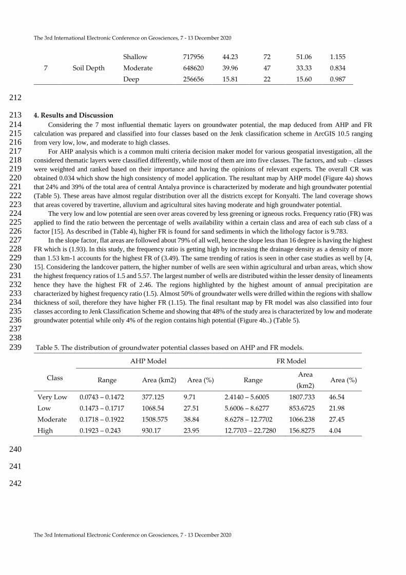
Considering the 7 most influential thematic layers on groundwater potential, the map deduced from AHP and FR 214 calculation was prepared and classified into four classes based on the Jenk classification scheme in ArcGIS 10.5 ranging 215 from very low, low, and moderate to high classes. 216
For AHP analysis which is a common multi criteria decision maker model for various geospatial investigation, all the 217 considered thematic layers were classified differently, while most of them are into five classes. The factors, and sub – classes 218 were weighted and ranked based on their importance and having the opinions of relevant experts. The overall CR was 219 obtained 0.034 which show the high consistency of model application. The resultant map by AHP model (Figure 4a) shows 220 that 24% and 39% of the total area of central Antalya province is characterized by moderate and high groundwater potential 221 (Table 5). These areas have almost regular distribution over all the districts except for Konyalti. The land coverage shows 222 that areas covered by travertine, alluvium and agricultural sites having moderate and high groundwater potential. 223 The very low and low potential are seen over areas covered by less greening or igneous rocks. Frequency ratio (FR) was 224 applied to find the ratio between the percentage of wells availability within a certain class and area of each sub class of a 225 factor [15]. As described in (Table 4), higher FR is found for sand sediments in which the lithology factor is 9.783. 226 In the slope factor, flat areas are followed about 79% of all well, hence the slope less than 16 degree is having the highest 227 FR which is (1.93). In this study, the frequency ratio is getting high by increasing the drainage density as a density of more 228 than 1.53 km-1 accounts for the highest FR of (3.49). The same trending of ratios is seen in other case studies as well by [4, 229 15]. Considering the landcover pattern, the higher number of wells are seen within agricultural and urban areas, which show 230 the highest frequency ratios of 1.5 and 5.57. The largest number of wells are distributed within the lesser density of lineaments 231 hence they have the highest FR of 2.46. The regions highlighted by the highest amount of annual precipitation are 232 characterized by highest frequency ratio (1.5). Almost 50% of groundwater wells were drilled within the regions with shallow 233 thickness of soil, therefore they have higher FR (1.15). The final resultant map by FR model was also classified into four 234 classes according to Jenk Classification Scheme and showing that 48% of the study area is characterized by low and moderate 235 groundwater potential while only 4% of the region contains high potential (Figure 4b..) (Table 5). 236 237 238
Table 5. The distribution of groundwater potential classes based on AHP and FR models. 239
Class
AHP Model FR Model
Range Area (km2) Area (%) Range Area
(km2) Area (%)
Very Low 0.0743 – 0.1472 377.125 9.71 2.4140 – 5.6005 1807.733 46.54
Low 0.1473 – 0.1717 1068.54 27.51 5.6006 – 8.6277 853.6725 21.98
Moderate 0.1718 – 0.1922 1508.575 38.84 8.6278 – 12.7702 1066.238 27.45
High 0.1923 – 0.243 930.17 23.95 12.7703 – 22.7280 156.8275 4.04
240
241
242
The 3rd International Electronic Conference on Geosciences, 7 - 13 December 2020
The 3rd International Electronic Conference on Geosciences, 7 - 13 December 2020
243
Figure 4. The groundwater potential maps for central Antalya, Turkey by a) AHP Model, b) FR Model. 244
245
4.1. Validation 246
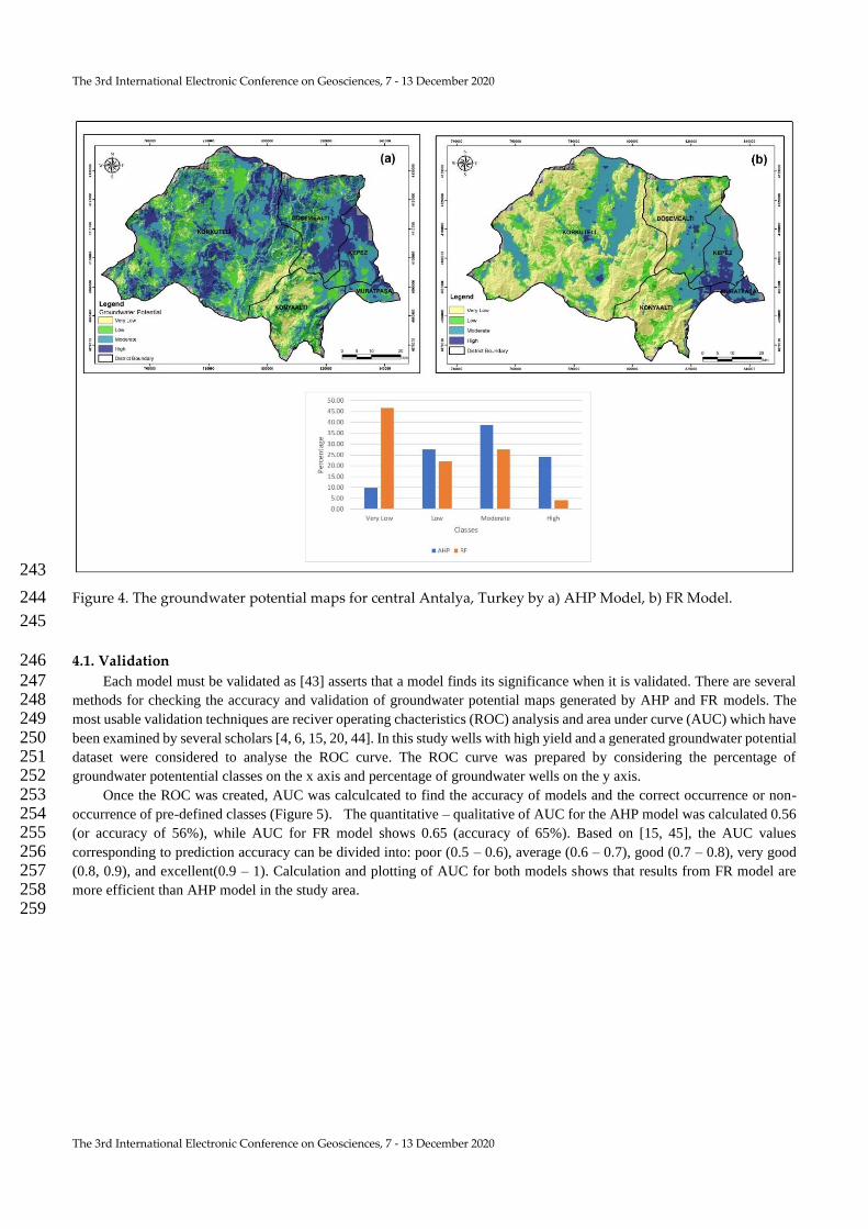
Each model must be validated as [43] asserts that a model finds its significance when it is validated. There are several 247 methods for checking the accuracy and validation of groundwater potential maps generated by AHP and FR models. The 248 most usable validation techniques are reciver operating chacteristics (ROC) analysis and area under curve (AUC) which have 249 been examined by several scholars [4, 6, 15, 20, 44]. In this study wells with high yield and a generated groundwater potential 250 dataset were considered to analyse the ROC curve. The ROC curve was prepared by considering the percentage of 251 groundwater potentential classes on the x axis and percentage of groundwater wells on the y axis. 252
Once the ROC was created, AUC was calculcated to find the accuracy of models and the correct occurrence or non-253 occurrence of pre-defined classes (Figure 5). The quantitative – qualitative of AUC for the AHP model was calculated 0.56 254 (or accuracy of 56%), while AUC for FR model shows 0.65 (accuracy of 65%). Based on [15, 45], the AUC values 255 corresponding to prediction accuracy can be divided into: poor (0.5 – 0.6), average (0.6 – 0.7), good (0.7 – 0.8), very good 256 (0.8, 0.9), and excellent(0.9 – 1). Calculation and plotting of AUC for both models shows that results from FR model are 257 more efficient than AHP model in the study area. 258
259

The 3rd International Electronic Conference on Geosciences, 7 - 13 December 2020
The 3rd International Electronic Conference on Geosciences, 7 - 13 December 2020
260
261
Figure 5. Chart showing the ROC curve and AUC for AHP and FR models 262
263
264
5. Conclusions 265
Groundwater potential mapping has been carried out using different traditional and remotely based approaches for 266 decades. The use of remote sensing technology and GIS makes it easy and accessible for experts to conduct potential mapping 267 with low effective costs and time consumed. Various spatial and non-spatial modelling using GIS environment are applied 268 to demarcate groundwater potential in which their accuracy is different. In this study, analytical hierarchy process and 269 frequency ratio models were applied by considering seven thematic layers: lithology, slope, drainage density, 270 landcover/landuse, lineament density, rainfall, and soil depth. 271
By giving high importance to lithology of the region and less importance to the soil depth layer, Muratpasa, Kepez, and 272 eastern Dosemealti districts are followed by the high potential of groundwater based on both models. The main reasons for 273 high potential of these districts are existence of a huge travertine plateau which makes an environment for higher permeability 274 of groundwater. The regions are characterized by steep slopes, also igneous rocks coverage is directed to low and very low 275 groundwater potential due to huge amounts of run off on the surface. The regions covered by agricultural, forest areas and 276 alluvium have moderate potential for groundwater. 277
The reliability of the AHP model for groundwater potential demarcation is directly dependent on the assignment of the 278 weights and ranks to each class and sub-class. Therefore, deep study and knowledge on factors influencing the targeted object 279 are required, also the geographical, geological, and hydrological characteristics of the study area are another point to be 280 contemplated. Implementation of FR does not require more knowledge of users to set ranks or weights, while the model itself 281 finds ratio of factors which gives more reliable results. The final resultants maps and validation confirm that groundwater 282 potential mapped by FR is more reliable and efficient than the AHP model. The results from this study can be a hint for the 283 responsible departments to have accurate future planning of groundwater in terms of distribution, planning, consumption, 284 and artificial recharge. Moreover, the findings should be followed with further detailed field work and other relevant studies 285 to accomplish accurate groundwater potential mapping at large scale over the small districts and villages. 286
287 Conflict of interest 288 The authors declare that there is not any potential conflict arising out of this paper. The paper is also not accompanied 289
by any funding resources. 290
References 291
1. Fitts C (2002) Groundwater science 292
2. Bagyaraj M, Ramkumar T, Venkatramanan S, Gurugnanam B (2013) Application of remote sensing and 293
GIS analysis for identifying groundwater potential zone in parts of Kodaikanal Taluk, South India. Front 294
Earth Sci 7:65–75. https://doi.org/10.1007/s11707-012-0347-6 295
0
0.2
0.4
0.6
0.8
1
0 0.2 0.4 0.6 0.8 1
Wel
l Dis
trib
uti
on
Per
cen
tage
Area Percentage
FR (65%)
AHP (56%)
The 3rd International Electronic Conference on Geosciences, 7 - 13 December 2020
The 3rd International Electronic Conference on Geosciences, 7 - 13 December 2020
3. Naghibi SA, Pourghasemi HR, Pourtaghi ZS, Rezaei A (2015) Groundwater qanat potential mapping using 296
frequency ratio and Shannon’s entropy models in the Moghan watershed, Iran. Earth Sci Informatics 297
8:171–186. https://doi.org/10.1007/s12145-014-0145-7 298
4. Das S (2019) Comparison among influencing factor, frequency ratio, and analytical hierarchy process 299
techniques for groundwater potential zonation in Vaitarna basin, Maharashtra, India. Groundw Sustain 300
Dev 8:617–629. https://doi.org/10.1016/j.gsd.2019.03.003 301
5. Todd D, Mays L (2004) Groundwater hydrology 302
6. Manap MA, Sulaiman WNA, Ramli MF, et al (2013) A knowledge-driven GIS modeling technique for 303
groundwater potential mapping at the Upper Langat Basin, Malaysia. Arab J Geosci 6:1621–1637. 304
https://doi.org/10.1007/s12517-011-0469-2 305
7. Senanayake IP, Dissanayake DMDOK, Mayadunna BB, Weerasekera WL (2016) An approach to delineate 306
groundwater recharge potential sites in Ambalantota, Sri Lanka using GIS techniques. Geosci Front 7:115–307
124. https://doi.org/10.1016/j.gsf.2015.03.002 308
8. Banks D, Robins N (2002) An introduction to Groundwater in Crystalline Bedrock 309
9. Mukherjee S (1996) Targeting saline aquifer by remote sensing and geophysical methods in a part of 310
Hamirpur-Kanpur, India. Hydrogeol J 19:53–64 311
10. Ganapuram S, Kumar GTV, Krishna IVM, et al (2009) Mapping of groundwater potential zones in the 312
Musi basin using remote sensing data and GIS. Adv Eng Softw 40:506–518. 313
https://doi.org/10.1016/j.advengsoft.2008.10.001 314
11. Oh HJ, Kim YS, Choi JK, et al (2011) GIS mapping of regional probabilistic groundwater potential in the 315
area of Pohang City, Korea. J Hydrol 399:158–172. https://doi.org/10.1016/j.jhydrol.2010.12.027 316
12. Das S, Pardeshi SD (2018) Integration of different influencing factors in GIS to delineate groundwater 317
potential areas using IF and FR techniques: a study of Pravara basin, Maharashtra, India. Appl Water Sci 318
8:. https://doi.org/10.1007/s13201-018-0848-x 319
13. Jha MK, Chowdary VM, Chowdhury A (2010) Groundwater assessment in Salboni Block, West Bengal 320
(India) using remote sensing, geographical information system and multi-criteria decision analysis 321
techniques. Hydrogeol J 18:1713–1728. https://doi.org/10.1007/s10040-010-0631-z 322
14. Nampak H, Pradhan B, Manap MA (2014) Application of GIS based data driven evidential belief function 323
model to predict groundwater potential zonation. J Hydrol 513:283–300. 324
https://doi.org/10.1016/j.jhydrol.2014.02.053 325
15. Razandi Y, Pourghasemi HR, Neisani NS, Rahmati O (2015) Application of analytical hierarchy process, 326
frequency ratio, and certainty factor models for groundwater potential mapping using GIS. Earth Sci 327
Informatics 8:867–883. https://doi.org/10.1007/s12145-015-0220-8 328
16. Al-Shabeeb AAR, Al-Adamat R, Al-Fugara A, et al (2018) Delineating groundwater potential zones within 329
the Azraq Basin of Central Jordan using multi-criteria GIS analysis. Groundw Sustain Dev 7:82–90. 330
https://doi.org/10.1016/j.gsd.2018.03.011 331
17. Jasrotia AS, Kumar R, Saraf AK, et al (2007) International Journal of Remote Sensing Delineation of 332
groundwater recharge sites using integrated remote sensing and GIS in Jammu district, India Delineation 333
of groundwater recharge sites using integrated remote sensing and GIS in Jammu district, India. Taylor 334
Fr 28:5019–5036. https://doi.org/10.1080/01431160701264276 335
18. Magesh NS, Chandrasekar N, Soundranayagam JP (2012) Delineation of groundwater potential zones in 336
Theni district, Tamil Nadu, using remote sensing, GIS and MIF techniques. Geosci Front 3:189–196. 337
https://doi.org/10.1016/j.gsf.2011.10.007 338
The 3rd International Electronic Conference on Geosciences, 7 - 13 December 2020
The 3rd International Electronic Conference on Geosciences, 7 - 13 December 2020
19. Naghibi SA, Moradi Dashtpagerdi M (2017) Evaluation of four supervised learning methods for 339
groundwater spring potential mapping in Khalkhal region (Iran) using GIS-based features. Hydrogeol J 340
25:169–189. https://doi.org/10.1007/s10040-016-1466-z 341
20. Ozdemir A (2011) GIS-based groundwater spring potential mapping in the Sultan Mountains (Konya, 342
Turkey) using frequency ratio, weights of evidence and logistic regression methods and their comparison. 343
J Hydrol 411:290–308. https://doi.org/10.1016/j.jhydrol.2011.10.010 344
21. Sener E, Davraz A (2013) Assessment of groundwater vulnerability based on a modified DRASTIC model, 345
GIS and an analytic hierarchy process (AHP) method: The case of Egirdir Lake basin (Isparta, Turkey). 346
Hydrogeol J 21:701–714. https://doi.org/10.1007/s10040-012-0947-y 347
22. Rahmati O, Nazari Samani A, Mahdavi M, et al (2015) Groundwater potential mapping at Kurdistan 348
region of Iran using analytic hierarchy process and GIS. Arab J Geosci 8:7059–7071. 349
https://doi.org/10.1007/s12517-014-1668-4 350
23. Hossein A, Ardakani H, Ekhtesasi MR (2016) Groundwater potentiality through Analytic Hierarchy 351
Process (AHP) using remote sensing and Geographic Information System (GIS) 352
24. Jenifer MA, Jha MK (2017) Comparison of Analytic Hierarchy Process, Catastrophe and Entropy 353
techniques for evaluating groundwater prospect of hard-rock aquifer systems. J Hydrol 548:605–624. 354
https://doi.org/10.1016/j.jhydrol.2017.03.023 355
25. Guru B, Seshan K, Bera S (2017) Frequency ratio model for groundwater potential mapping and its 356
sustainable management in cold desert, India. J. King Saud Univ. - Sci. 29:333–347 357
26. Şener E, Şener Ş, Davraz A (2018) Groundwater potential mapping by combining fuzzy-analytic hierarchy 358
process and GIS in Beyşehir Lake Basin, Turkey. Arab J Geosci 11:. https://doi.org/10.1007/s12517-018-359
3510-x 360
27. Mogaji KA, Lim HS, Abdullah K (2015) Regional prediction of groundwater potential mapping in a 361
multifaceted geology terrain using GIS-based Dempster–Shafer model. Arab J Geosci 8:3235–3258. 362
https://doi.org/10.1007/s12517-014-1391-1 363
28. Naghibi SA, Pourghasemi HR, Dixon B (2016) GIS-based groundwater potential mapping using boosted 364
regression tree, classification and regression tree, and random forest machine learning models in Iran. 365
Environ Monit Assess 188:1–27. https://doi.org/10.1007/s10661-015-5049-6 366
29. Zabihi M, Pourghasemi HR, Pourtaghi ZS, Behzadfar M (2016) GIS-based multivariate adaptive regression 367
spline and random forest models for groundwater potential mapping in Iran. Environ Earth Sci 75:. 368
https://doi.org/10.1007/s12665-016-5424-9 369
30. Chen W, Li H, Hou E, et al (2018) GIS-based groundwater potential analysis using novel ensemble 370
weights-of-evidence with logistic regression and functional tree models. Sci Total Environ 634:853–867. 371
https://doi.org/10.1016/j.scitotenv.2018.04.055 372
31. Lee S, Hong SM, Jung HS (2018) GIS-based groundwater potential mapping using artificial neural network 373
and support vector machine models: the case of Boryeong city in Korea. Geocarto Int 33:847–861. 374
https://doi.org/10.1080/10106049.2017.1303091 375
32. Golkarian A, Rahmati O (2018) Use of a maximum entropy model to identify the key factors that influence 376
groundwater availability on the Gonabad Plain, Iran. Environ Earth Sci 77:. https://doi.org/10.1007/s12665-377
018-7551-y 378
33. Prasad RK, Mondal NC, Banerjee P, et al (2008) Deciphering potential groundwater zone in hard rock 379
through the application of GIS. Environ Geol 55:467–475. https://doi.org/10.1007/s00254-007-0992-3 380
34. Dinesh Kumar PK, Gopinath G, Seralathan P (2007) International Journal of Remote Sensing Application 381

The 3rd International Electronic Conference on Geosciences, 7 - 13 December 2020
The 3rd International Electronic Conference on Geosciences, 7 - 13 December 2020
of remote sensing and GIS for the demarcation of groundwater potential zones of a river basin in Kerala, 382
southwest coast of India Application of remote sensing and GIS for the demarcation of groundwater . Int 383
J Remote Sens 28:5583–5601. https://doi.org/10.1080/01431160601086050 384
35. Saha D, Dhar Y, assessment SV-E monitoring and, 2010 undefined (2010) Delineation of groundwater 385
development potential zones in parts of marginal Ganga Alluvial Plain in South Bihar, Eastern India. 386
Springer 165:179–191. https://doi.org/10.1007/s10661-009-0937-2 387
36. Adiat KAN, Nawawi MNM, Abdullah K (2012) Assessing the accuracy of GIS-based elementary multi 388
criteria decision analysis as a spatial prediction tool - A case of predicting potential zones of sustainable 389
groundwater resources. J Hydrol 440–441:75–89. https://doi.org/10.1016/j.jhydrol.2012.03.028 390
37. Saaty T (1990) Decision making for leaders: the analytic hierarchy process for decisions in a complex world 391
38. Kumar A, Krishna AP (2018) Assessment of groundwater potential zones in coal mining impacted hard-392
rock terrain of India by integrating geospatial and analytic hierarchy process (AHP) approach. Geocarto 393
Int 33:105–129. https://doi.org/10.1080/10106049.2016.1232314 394
39. Hosseinali F, Alesheikh AA (2008) Weighting spatial information in GIS for copper mining exploration. 395
Am J Appl Sci 5:1187–1198. https://doi.org/10.3844/ajassp.2008.1187.1198 396
40. Malczewski J (1999) GIS and multicriteria decision analysis 397
41. Saaty TL (1977) A scaling method for priorities in hierarchical structures. J Math Psychol 15:234–281. 398
https://doi.org/10.1016/0022-2496(77)90033-5 399
42. Bonham-Carter, F G (1994) Geographic information systems for geoscientists: Modelling with GIS. 400
Comput methods Geosci 13:398. https://doi.org/10.1016/0098-3004(95)90019-5 401
43. Fabbri A, Chung C-JF, Fabbri AG (2003) Validation of Spatial Prediction Models for Landslide Hazard 402
Mapping. Nat Hazards 30:451–472. https://doi.org/10.1023/B:NHAZ.0000007172.62651.2b 403
44. Andualem TG, Demeke GG (2019) Groundwater potential assessment using GIS and remote sensing: A 404
case study of Guna tana landscape, upper blue Nile Basin, Ethiopia. J Hydrol Reg Stud 24:. 405
https://doi.org/10.1016/j.ejrh.2019.100610 406
45. Yesilnacar E (2005) The application of computational intelligence to landslide susceptibility mapping in 407 Turkey. Univ Melbourne, PhD Thesis 408
© 2020 by the authors; licensee MDPI, Basel, Switzerland. This article is an open access article 409 distributed under the terms and conditions of the Creative Commons by Attribution (CC-BY) 410 license (http://creativecommons.org/licenses/by/4.0/). 411