BART: Bayesian Additive Regression Trees

Robert McCulloch

McCombs School of BusinessUniversity of Texas

May 11, 2011

Joint withHugh Chipman (Acadia University)

Ed George (University of Pennsylvania)

We want to “fit” the fundamental model:

Yi = f (Xi ) + εi

BART is a Markov Monte Carlo Method that draws from

f | (x , y)

We can then use the draws as our inference for f .

To get the draws, we will have to:

I Put a prior on f .

I Specify a Markov chain whose stationary distribution is theposterior of f .

Simulate data from the model:

Yi = x3i + εi εi ∼ N(0, σ2) iid

--------------------------------------------------n = 100sigma = .1f = function(x) {x^3}set.seed(14)x = sort(2*runif(n)-1)y = f(x) + sigma*rnorm(n)xtest = seq(-1,1,by=.2)--------------------------------------------------

Here, xtest will be the out of sample x values at which we wish toinfer f or make predictions.

--------------------------------------------------plot(x,y)points(xtest,rep(0,length(xtest)),col=’red’,pch=16)--------------------------------------------------

●

●

●

●

●

●

●

●

●●●●

●

●

●●

●

●

●

●

●●

●●●

●

●

●

●

●●

●

●

●●

●

●

●

●

●

●

●●

●

●●●

●

●

●

●

●

●

●

●●

●

●

●

●

●

●

●

●

●

●

●

●

●

●

●●

●

●

●

●

●

●

●

● ●

●

●

●

●●

●●

●

●

●

●

●

●●●

●●

●

●

−1.0 −0.5 0.0 0.5 1.0

−1.

0−

0.5

0.0

0.5

1.0

x

y

● ● ● ● ● ● ● ● ● ● ●

Red is xtest.

--------------------------------------------------library(BayesTree)rb = bart(x,y,xtest)length(xtest)[1] 11dim(rb$yhat.test)[1] 1000 11--------------------------------------------------

The (i , j) element of yhat.test is

the i th draw of f evaluated at the j th value of xtest.

1,000 draws of f , each of which is evaluated at 11 xtest values.

--------------------------------------------------

plot(x,y)

lines(xtest,xtest^3,col=’blue’)

lines(xtest,apply(rb$yhat.test,2,mean),col=’red’)

qm = apply(rb$yhat.test,2,quantile,probs=c(.05,.95))

lines(xtest,qm[1,],col=’red’,lty=2)

lines(xtest,qm[2,],col=’red’,lty=2)

--------------------------------------------------

●

●

●

●

●

●

●

●

●●●●

●

●

●●

●

●

●

●

●●

●●●

●

●

●

●

●●

●

●

●●

●

●

●

●

●

●

●●

●

●●●

●

●

●

●

●

●

●

●●

●

●

●

●

●

●

●

●

●

●

●

●

●

●

●●

●

●

●

●

●

●

●

● ●

●

●

●

●●

●●

●

●

●

●

●

●●●

●●

●

●

−1.0 −0.5 0.0 0.5 1.0

−1.

0−

0.5

0.0

0.5

1.0

x

y

Example: Out of Sample Prediction

Did out of sample predictive comparisons on 42 data sets.(thanks to Wei-Yin Loh!!)

I p=3− 65, n = 100− 7, 000.I for each data set 20 random splits into 5/6 train and 1/6 testI use 5-fold cross-validation on train to pick hyperparameters (except

BART-default!)I gives 20*42 = 840 out-of-sample predictions, for each prediction, divide rmse

of different methods by the smallest

+ each boxplots represents840 predictions for amethod

+ 1.2 means you are 20%worse than the best

+ BART-cv best

+ BART-default (use defaultprior) does amazinglywell!!

Ron

dom

For

ests

Neu

ral N

etB

oost

ing

BA

RT

−cv

BA

RT

−de

faul

t

1.0 1.1 1.2 1.3 1.4 1.5

A Regression Tree Model

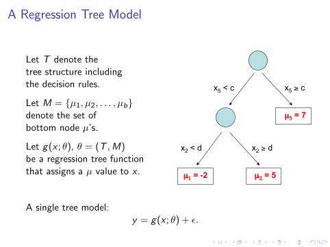
Let T denote thetree structure includingthe decision rules.

Let M = {µ1, µ2, . . . , µb}denote the set ofbottom node µ’s.

Let g(x ; θ), θ = (T ,M)be a regression tree functionthat assigns a µ value to x .

A Single Regression Tree Model

x2 < d x2 % d

x5 < c x5 % c

µ3 = 7

µ1 = -2 µ2 = 5

Let g(x;"), " = (T, M) be a regression tree function that assigns a µ value to x

Let T denote the tree structure including the decision rules

Let M = {µ1, µ2, … µb} denote the set of bottom node µ's.

A Single Tree Model: Y = g(x;!) + ! 7

A single tree model:y = g(x ; θ) + ε.

A coordinate view of g(x ; θ)

The Coordinate View of g(x;")

x2 < d x2 % d

x5 < c x5 % c

µ3 = 7

µ1 = -2 µ2 = 5

Easy to see that g(x;") is just a step function

µ1 = -2 µ2 = 5

⇔ µ3 = 7

c

d x2

x5

8

Easy to see that g(x ; θ) is just a step function.

The BART ModelLet " = ((T1,M1), (T2,M2), …, (Tm,Mm)) identify a set of m trees and their µ’s.

Y = g(x;T1,M1) + g(x;T2,M2) + ... + g(x;Tm,Mm) + ! z, z ~ N(0,1)

The BART Ensemble Model

E(Y | x, ") is the sum of all the corresponding µ’s at each tree bottom node.

Such a model combines additive and interaction effects.

µ1

µ2 µ3

µ4

9 Remark: We here assume ! ~ N(0, !2) for simplicity, but will later see a successful extension to a general DP process model.

m = 200, 1000, . . . , big, . . ..

f (x | ·) is the sum of all the corresponding µ’s at each bottomnode.

Such a model combines additive and interaction effects.

Complete the Model with a Regularization Prior

π(θ) = π((T1,M1), (T2,M2), . . . , (Tm,Mm), σ).

π wants:

I Each T small.

I Each µ small.

I “nice” σ (smaller than least squares estimate).

We refer to π as a regularization prior because it keeps the overallfit small.

In addition, it keeps the contribution of each g(x ; Ti ,Mi ) modelcomponent small.

Consider the prior on µ.Let θ denote all the parameters.

f (x | θ) = µ1 + µ2 + · · ·µm.

Let µi ∼ N(0, σ2µ), iid.

f (x | θ) ∼ N(0,m σ2µ).

In practice we often, unabashadly, use the data by first centeringand then choosing σµ so that

f (x | θ) ∈ (ymin, ymax)

with high probability:

σ2µ ∝

1

m.

BART MCMC

Bayesian Nonparametrics: Lots of parameters (to make model flexible) A strong prior to shrink towards simple structure (regularization) BART shrinks towards additive models with some interaction

Dynamic Random Basis: g(x;T1,M1), ..., g(x;Tm,Mm) are dimensionally adaptive

Gradient Boosting: Overall fit becomes the cumulative effort of many “weak learners”

Connections to Other Modeling Ideas

Y = g(x;T1,M1) + ... + g(x;Tm,Mm) + & z plus

#((T1,M1),....(Tm,Mm),&)

12

First, it is a “simple” Gibbs sampler:

(Ti ,Mi ) | (T1,M1, . . . ,Ti−1,Mi−1,Ti+1,Mi+1, . . . ,Tm,Mm, σ)

σ | (T1,M1, . . . , . . . ,Tm,Mm)

To draw (Ti ,Mi ) | · we subract the contributions of the othertrees from both sides to get a simple one-tree model.

We integrate out M to draw T and then draw M | T .

To draw T we use a Metropolis-Hastings with Gibbs step.We use various moves, but the key is a “birth-death” step.Because p(T | data) is available in closed form (up to a norming constant),

we use a Metropolis-Hastings algorithm.

Our proposal moves around tree space by proposing local modifications such as

=> ?

=> ?

propose a more complex tree

propose a simpler tree

Such modifications are accepted according to their compatibility with p(T | data). 20

Simulating p(T | data) with the Bayesian CART Algorithm

Bayesian Nonparametrics: Lots of parameters (to make model flexible) A strong prior to shrink towards simple structure (regularization) BART shrinks towards additive models with some interaction

Dynamic Random Basis: g(x;T1,M1), ..., g(x;Tm,Mm) are dimensionally adaptive

Gradient Boosting: Overall fit becomes the cumulative effort of many “weak learners”

Connections to Other Modeling Ideas

Y = g(x;T1,M1) + ... + g(x;Tm,Mm) + & z plus

#((T1,M1),....(Tm,Mm),&)

12

Connections to Other Modeling Ideas:

Bayesian Nonparametrics:- Lots of parameters to make model flexible.- A strong prior to shrink towards a simple structure.- BART shrinks towards additive models with some interaction.

Dynamic Random Basis:- g(x ; T1,M1), g(x ; T2,M2), . . . , g(x ; Tm,Mm) are

dimensionally adaptive.

Gradient Boosting:- Overall fit becomes the cumulative effort

of many weak learners.

Bayesian Nonparametrics: Lots of parameters (to make model flexible) A strong prior to shrink towards simple structure (regularization) BART shrinks towards additive models with some interaction

Dynamic Random Basis: g(x;T1,M1), ..., g(x;Tm,Mm) are dimensionally adaptive

Gradient Boosting: Overall fit becomes the cumulative effort of many “weak learners”

Connections to Other Modeling Ideas

Y = g(x;T1,M1) + ... + g(x;Tm,Mm) + & z plus

#((T1,M1),....(Tm,Mm),&)

12

Some Distinguishing Feastures of BART:

BART is NOT Bayesian model averaging of single tree model.

Unlike Boosting and Random Forests, BART updates a set of mtrees over and over, stochastic search.

Choose m large for flexible estimation and prediction.

Choose m smaller for variable selection- fewer trees forces the x ’s to compete for entry.

The Friedman Simulated Example

y = f (x) + Z , Z ∼ N(0, 1).

f (x) = 10 sin(πx1x2) + 20(x3 − .5)2 + 10x4 + 5x5.

n = 100.Add 5 irrelevant x ’s (p = 10).xi ∼ uniform(0, 1).f (x) is the posterior mean.

Compute out of sample RMSE using 1,000 simulated x ∈ R10.

RMSE =

√√√√ 1

1000

1000∑i=1

(f (xi )− f (xi ))2

Performance measured on 1000 out-of-sample x’s by

Comparison of BART with Other Methods

28

Cross Validation Domain for Comparisons

29

Results for one draw.

Applying BART to the Friedman Example

Red m = 1 model

Blue m = 100 model

We applied BART with m = 100 trees to n = 100 observations of the Friedman example.

95% posterior intervals vs true f(x) & draws

in-sample f(x) out-of-sample f(x) MCMC iteration

30 Frequentist coverage rates of 90% posterior intervals:in sample: 87%out of sample: 93 %.

With only 100 observations on y and 1000 x's, BART yielded "reasonable" results !!!!

Added many useless x's to Friedman’s example

In-sample post int vs f(x)

20 x's

100 x's

1000 x's

Detecting Low Dimensional Structure in High Dimensional Data Out-of-sample post int vs f(x) & draws

31

Big p, small n.

n = 100.

Compare BART-default,BART-cv,boosting, random forests.

Out of sample RMSE.

High Dimensional Out-of-Sample RMSE Performance Comparisons

p = 10 p = 100 p = 1000

n = 100 throughout!

32

Partial Dependence plot:

Vary one x and average out the others.

Partial Dependence Plots for the Friedman Example The Marginal Effects of x1 – x10

41

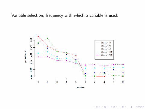
Variable selection, frequency with which a variable is used.Variable Selection via BART

Variable usage frequencies as the number of trees m is reduced

38

Example: Drug Discovery

Goal: To predict the “activity” of a compound against a biologicaltarget.

That is: y = 1 means drug worked (compound active), 0 means itdoes not.

Easy to extend BART to binary y using Albert & Chib.

n = 29, 3744→ 14, 687 train, 14, 687 test.p = 266 characterizations of the compound’s molecular structure.

Again, out-of-sample prediction competitive with other methods,compared to neural-nets, boosting, random forests, support vectormachines.

20 compounds with highest Pr(Y = 1 | x) estimate.90% posterior intervals for Pr(Y = 1 | x).

BART Posterior Intervals for 20 Compounds with Highest Predicted Activity

In-sample Out-of-Sample

51

Variable selection.

Variable Importance in Drug Discovery with m = 5, 10, 20 trees

All 266 x’s Top 25 x’s

52

Current Work

Nonparametric modeling of the error distribution (with PaulDamien)

Multinomial outcomes (with Nick Polson).

More on priors and variable-selection.

Constrain the multivariate function to be monotonic(with Tom Shively)

- Tom has a beautiful cross-dimensional,constrained, slice-sampler.

Recode with MPI to make it faster!!

With Dave Higdon, James Gattiker, and Matt Pratola at LosAlamos National Labs..

Dave came to me and said, “we tried your stuff (the R package)on the analysis of computer experiments and it seemed promisingbut it is too slow”.

1. Rewrote code so that it is leaner.

2. Used MPI to compute.

num obs new-parallel new-serial old

1 1000 7 9 43

2 2000 8 18 95

3 3000 9 28 149

4 4000 10 36 204

5 5000 12 45 262

6 10000 18 90 547

7 50000 70 439 NA

8 100000 138 902 NA

9 500000 904 6410 NA

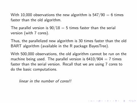
With 10,000 observations the new algorithm is 547/90 = 6 timesfaster than the old algorithm.

The parallel version is 90/18 = 5 times faster than the serialversion (with 7 cores).

Thus, the parallelized new algorithm is 30 times faster than the oldBART algorithm (available in the R package BayesTree).

With 500,000 observations, the old algorithm cannot be run on themachine being used. The parallel version is 6410/904 = 7 timesfaster than the serial version. Recall that we are using 7 cores todo the basic computations.

linear in the number of cores!!

100,000 observations, p = 251.For regression, cor(y , y) = .84 for BART = .99.

Blue is BART, red is least-squares.

1.1 1.2 1.3 1.4 1.5 1.6

1.1

1.2

1.3

1.4

1.5

1.6

y, n=2000

fits

bart=blue,reg=red

1.1 1.2 1.3 1.4 1.5 1.6

1.0

1.1

1.2

1.3

1.4

1.5

1.6

y, n=5000

fits

3. Parallelize prediction, so we can do all the stuff we want!