Banking Stability Mea sures...514 Banking Stability Mea sures cycle.4 Consequently, the proposed BSMs represent a set of tools to analyze (defi ne) stability from four diff erent yet

CHAPTER 32

Banking Stability Mea sures

MIGUEL A. SEGOVIANO • CHARLES A. E. GOODHART

This chapter defi nes a set of banking stability mea sures that take account of distress dependence among the banks in a system, thereby provid-ing a set of tools to analyze stability from complementary perspectives by allowing the mea sure ment of (1) common distress of the banks in a

system; (2) distress between specifi c banks; and (3) distress in the system associated with a specifi c bank. Our approach defi nes the banking system as a portfolio of banks and infers the Banking System’s (Portfolio) Multivariate Density (BSMD) from which the proposed mea sures are estimated. The BSMD embeds the banks’ default interdependence structure that captures linear and nonlinear distress dependencies among the banks in the system and its changes at diff erent times of the economic cycle. The BSMD is recovered using the Consistent Information Multivariate Density Op-timizing approach, a new approach that in the presence of restricted data improves density specifi cation without explicitly imposing parametric forms that, under restricted data sets, are diffi cult to model. Thus, the proposed mea sures can be constructed from a very limited set of publicly available data and can be provided for a wide range of both developing and developed economies.

METHOD SUMMARY

Overview Banking stability mea sures embed banks’ linear (correlation) and nonlinear distress dependence and their changes through the economic cycle. The approach defi nes the banking system as a portfolio of banks and infers its multivariate density from which the proposed mea sures are estimated. These can be provided for developed and developing economies and can be estimated under data- restricted environments.

Application The proposed stability mea sures incorporate changes in distress dependence that are consistent with the economic cycle; this is a key advantage over traditional risk models that typically incorporate only linear dependence (correlation structure) and assume it to be constant throughout the economic cycle. The framework is appropriate in situations where

1. data are limited; and 2. distress dependence among fi nancial institutions in a fi nancial system needs to be quantifi ed.

Nature of approach Statistical nonparametric density estimation.

Data requirements Probabilities of default (PDs): these can be market based (credit default swap spreads, bond spreads, structural models); they also can be estimated with supervisory information.

Stock prices of fi nancial institutions.

Strengths The framework allows the estimation of fi nancial stability mea sures that provide complementary perspectives on risk, with very limited data requirements. These mea sures can be updated with daily frequency.

Weaknesses It is necessary to have robust estimations of PDs. If PDs are not available, it is necessary to make assumptions about this variable.

Tool Proprietary estimation codes are available from the authors upon request. Contact author: M. Segoviano.

Th is chapter is an abridged version of IMF Working Paper No. 09/04 (Segoviano and Goodhart, 2009). Th e authors would like to thank S. Neftci, R. Rigobon, H. Shin, D. Tsomocos, M. Sydow, J. Fell, T. Bayoumi, K. Habermeier, and A. Tieman for helpful comments and discussions; and to acknowledge inputs from participants in the seminar series/conferences at the IMF, Eu ro pe an Central Bank, Morgan Stanley, Bank of En gland, Banca d’Italia, Columbia Univer-sity, Deutsche Bundesbank, Banque de France, and Riksbank.

Economics is a quantitative science. Macroeconomics de-pends on data for national income, expenditure, and output variables. Macromonetary policy requires mea sures of infl a-tion. Microeconomics is based on data for prices and quanti-

ties of inputs and outputs. Even when the variables of concern are diffi cult to mea sure, such as the output gap, expectations, and “happiness,” economists use various techniques, for ex-ample, survey data, to provide quantitative proxy variables—

536-57355_IMF_StressTestHBk_ch04_3P.indd 513 11/5/14 12:22 AM

Banking Stability Mea sures514

cycle.4 Consequently, the proposed BSMs represent a set of tools to analyze (defi ne) stability from four diff erent yet complementary perspectives, by allowing the quantifi cation of (1) “common” distress in the banks of the system, (2) dis-tress between specifi c banks, and (3) distress in the system associated with a specifi c bank.

In this chapter, we estimate the proposed BSMs using publicly available information from 2005 up to the begin-ning of October 2008. Th ese estimations are to illustrate the methodology rather than to make an assessment of the con-junctural fi nancial stability of any par tic u lar system. We ex-amine relative changes in stability over time and among diff erent banks’ business lines in the U.S. banking system. We also analyze cross- region eff ects between American and Eu ro pe an banking groups. Last, we show how our technique can be extended to incorporate the eff ect of foreign banks on sovereigns with banking systems with cross- border institu-tions. For this purpose, we estimate the BSMs for major for-eign banks and sovereigns in Latin America, Eastern Eu rope, and Asia. Th is implementation fl exibility is of relevance for banking stability surveillance, because cross- border fi nan-cial linkages are growing and becoming signifi cant, as has been highlighted by the fi nancial market turmoil of recent years. Th us, surveillance of banking stability cannot stop at national borders.

We show how these BSMs can be constructed from a very limited set of data, for example, empirical mea sure ments of distress of individual banks. Such mea sure ments can be esti-mated using alternative approaches, depending on data avail-ability; thus, the data set that is necessary to estimate the BSMs is available in most countries. Consequently, such mea-sures can be provided for a wide group of developing as well as developed economies. Establishing such a set of mea sures with a minimum of basic components makes it feasible to undertake a wider range of comparative analysis, both time series and cross section. It is important to note that when mea sure ments of distress of nonbanking fi nancial institutions (NBFIs), that is, insurance companies, hedge funds, and oth-ers, are available, our methodology can be extended easily to incorporate the eff ects of such institutions in the mea sure-ment of stability, hence allowing us to estimate a set of stabil-ity mea sures for the fi nancial system. Th is could be of relevance for countries where NBFIs have systemic importance in the fi nancial sector.

4 In contrast to correlation, which captures only linear dependence, cop-ula functions characterize the whole dependence structure— that is, linear and nonlinear dependence, embedded in multivariate densities (Nelsen, 1999). Th us, in order to characterize banks’ distress depen-dence, we employ a novel nonparametric copula approach, that is, the CIMDO copula. In comparison to traditional methodologies to model parametric copula functions, the CIMDO copula avoids the diffi culties of explicitly choosing the parametric form of the copula function to be used and calibrating its pa ram e ters, because CIMDO copula functions are inferred directly (implicitly) from the joint movements of the indi-vidual banks’ PoDs.

often according these data more weight than is consistent with their inherent mea sure ment errors. Without such quan-tifi cation, comparisons over time, and on a cross- sectional basis, cannot be made; nor would it be easy to provide a quantifi ed analysis of the determinants of such variables.

However, there is currently no such widely accepted mea-sure, quantifi cation, or time series for mea sur ing either fi nan-cial or banking stability. What is most often used instead is an on/off (1/0) assessment of whether a “crisis” has occurred.1 Th is then has been used to review whether there have been common factors preceding, possibly even causing, such cri-ses and to assess what offi cial responses have best mitigated such crises (see Hoelscher, 2006). Although much useful re-search employing a crisis on/off dichotomy has been done, this approach has several inherent defi ciencies.2 In par tic u-lar, the lack of a continuous scale makes it impossible to mea sure with suffi cient accuracy either (1) the relative riski-ness of the system in noncrisis mode; or (2) the intensity of a crisis once it has started. If the former could be mea sured, it may be easier to take early remedial action as the danger of a systemic crisis increases, while mea sure ment of the latter would facilitate decision making on the most appropriate mea sures to address the crisis.

In our view, a precondition for improving the analysis and management of fi nancial (banking) stability is to be able to construct a metric for it.3 Th e purpose of this study therefore is to present a method for estimating a set of sta-bility mea sures for the banking system, or banking stability mea sures (BSMs). Th ere is no unique, best way to estimate BSMs, any more than there is a unique best way to mea sure such concepts as “output” or “infl ation,” but we hope to demonstrate that our approach is reasonable. Moreover, there are very few alternative available mea sures that might be used.

Briefl y, and as described in far more detail in the subse-quent discussion, we conceptualize the banking system as a portfolio of banks comprising the core, systemically impor-tant banks in any country. Th us, we infer the Banking Sys-tem’s (Portfolio) Multivariate Density (BSMD), from which we construct a set of BSMs. Th ese mea sures embed the banks’ distress interdependence structure, which captures not only linear (correlation) but also nonlinear distress dependencies among the banks in the system. Moreover, the structure of linear and nonlinear distress dependencies changes as banks’ probabilities of distress (PoDs) change; hence, the proposed stability mea sures incorporate changes in distress depen-dence that are consistent with the economic cycle. Th is is a key advantage over traditional risk models that most of the time incorporate only linear dependence (correlation structure) and assume it constant throughout the economic

1 For a review of the literature on fi nancial crises, see Bordo and others (2001).

2 See Kaminsky and Reinhart (1999).3 See Kiyotaki and Moore (1997) and Krugman (1979).


Miguel A. Segoviano and Charles A. E. Goodhart 515

proposed BSMs are estimated. Th ese are defi ned in Section 3. In Section 4, we present empirical estimates of the pro-posed BSMs as described. Finally, conclusions are presented in Section 5.5

1. DISTRESS DEPENDENCE AMONG BANKS AND STABILITY OF THE BANKING SYSTEMTh e proper estimation of distress dependence among the banks in a system is of key importance for the surveillance of stability of the banking system. Financial supervisors recognize the importance of assessing not only the risk of distress— that is, large losses and possible default of a specifi c bank— but also the impact that such an event would have on other banks in the system. Clearly, the event of simultaneous large losses in various banks would aff ect a banking system’s stability and thus represents a major concern for supervisors. Banks’ distress dependence is based on the fact that banks are usually linked— either directly, through the interbank deposit market and participations in syndicated loans, or in-directly, through lending to common sectors and proprietary trades. Banks’ distress dependence varies across the eco-nomic cycle and tends to rise in times of distress because the fortunes of banks decline concurrently through either conta-gion after idiosyncratic shocks, aff ecting interbank deposit markets and participations in syndicated loans (direct links), or through negative systemic shocks, aff ecting lending to common sectors and proprietary trades (indirect links). Th ere-fore, in such periods, the banking system’s joint probability of distress ( JPoD)— that is, the probability that all the banks in the system experience large losses simultaneously, which embeds banks’ distress dependence— may experience larger and nonlinear increases than those experienced by the prob-abilities of distress (PoDs) of individual banks.

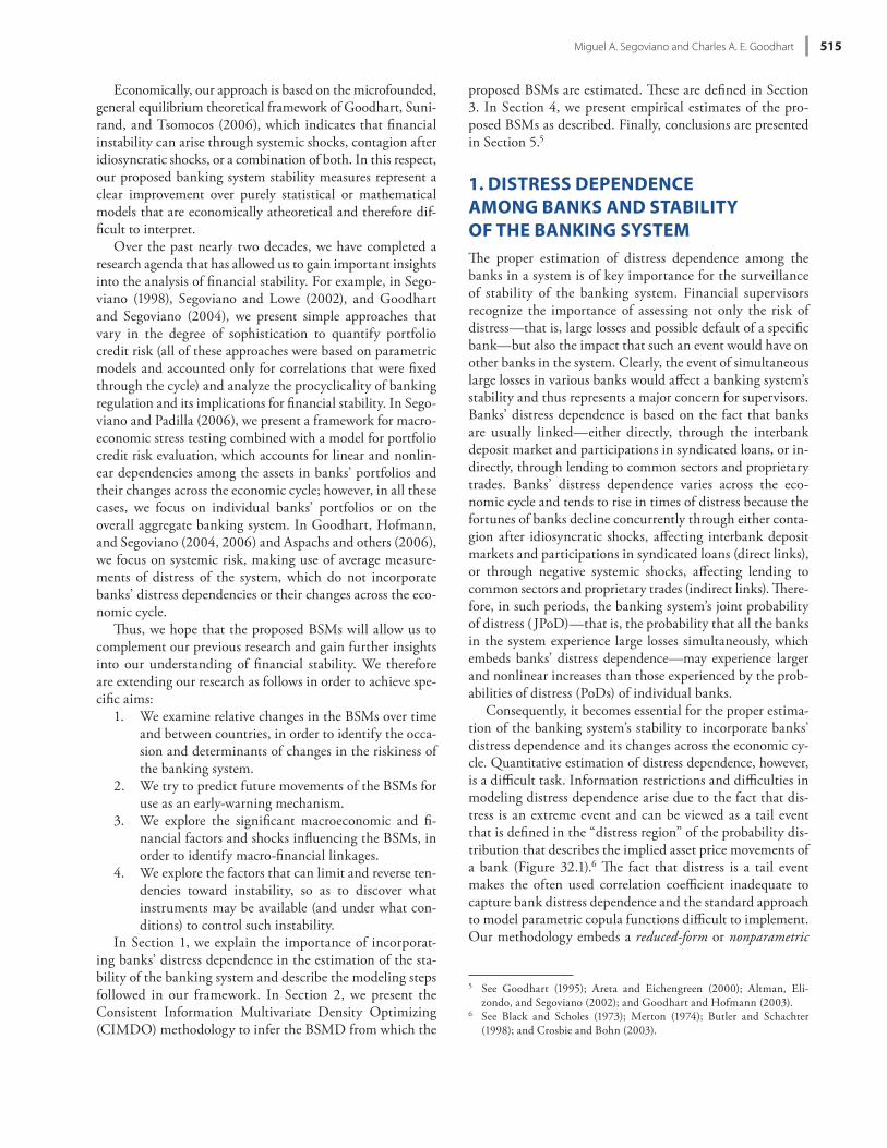
Consequently, it becomes essential for the proper estima-tion of the banking system’s stability to incorporate banks’ distress dependence and its changes across the economic cy-cle. Quantitative estimation of distress dependence, however, is a diffi cult task. Information restrictions and diffi culties in modeling distress dependence arise due to the fact that dis-tress is an extreme event and can be viewed as a tail event that is defi ned in the “distress region” of the probability dis-tribution that describes the implied asset price movements of a bank (Figure 32.1).6 Th e fact that distress is a tail event makes the often used correlation coeffi cient inadequate to capture bank distress dependence and the standard approach to model parametric copula functions diffi cult to implement. Our methodology embeds a reduced- form or nonparametric

5 See Goodhart (1995); Areta and Eichengreen (2000); Altman, Eli-zondo, and Segoviano (2002); and Goodhart and Hofmann (2003).

6 See Black and Scholes (1973); Merton (1974); Butler and Schachter (1998); and Crosbie and Bohn (2003).

Eco nom ical ly, our approach is based on the microfounded, general equilibrium theoretical framework of Goodhart, Suni-rand, and Tsomocos (2006), which indicates that fi nancial instability can arise through systemic shocks, contagion after idiosyncratic shocks, or a combination of both. In this respect, our proposed banking system stability mea sures represent a clear improvement over purely statistical or mathematical models that are eco nom ical ly atheoretical and therefore dif-fi cult to interpret.

Over the past nearly two de cades, we have completed a research agenda that has allowed us to gain important insights into the analysis of fi nancial stability. For example, in Sego-viano (1998), Segoviano and Lowe (2002), and Goodhart and Segoviano (2004), we present simple approaches that vary in the degree of sophistication to quantify portfolio credit risk (all of these approaches were based on parametric models and accounted only for correlations that were fi xed through the cycle) and analyze the procyclicality of banking regulation and its implications for fi nancial stability. In Sego-viano and Padilla (2006), we present a framework for macro-economic stress testing combined with a model for portfolio credit risk evaluation, which accounts for linear and nonlin-ear dependencies among the assets in banks’ portfolios and their changes across the economic cycle; however, in all these cases, we focus on individual banks’ portfolios or on the overall aggregate banking system. In Goodhart, Hofmann, and Segoviano (2004, 2006) and Aspachs and others (2006), we focus on systemic risk, making use of average mea sure-ments of distress of the system, which do not incorporate banks’ distress dependencies or their changes across the eco-nomic cycle.

Th us, we hope that the proposed BSMs will allow us to complement our previous research and gain further insights into our understanding of fi nancial stability. We therefore are extending our research as follows in order to achieve spe-cifi c aims:

1. We examine relative changes in the BSMs over time and between countries, in order to identify the occa-sion and determinants of changes in the riskiness of the banking system.

2. We try to predict future movements of the BSMs for use as an early- warning mechanism.

3. We explore the signifi cant macroeconomic and fi -nancial factors and shocks infl uencing the BSMs, in order to identify macro- fi nancial linkages.

4. We explore the factors that can limit and reverse ten-dencies toward instability, so as to discover what instruments may be available (and under what con-ditions) to control such instability.

In Section 1, we explain the importance of incorporat-ing banks’ distress dependence in the estimation of the sta-bility of the banking system and describe the modeling steps followed in our framework. In Section 2, we present the Consistent Information Multivariate Density Optimizing (CIMDO) methodology to infer the BSMD from which the



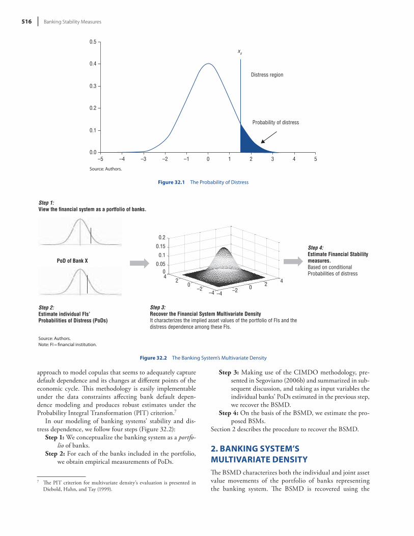
Step 3: Making use of the CIMDO methodology, pre-sented in Segoviano (2006b) and summarized in sub-sequent discussion, and taking as input variables the individual banks’ PoDs estimated in the previous step, we recover the BSMD.

Step 4: On the basis of the BSMD, we estimate the pro-posed BSMs.

Section 2 describes the procedure to recover the BSMD.

2. BANKING SYSTEM’S MULTIVARIATE DENSITYTh e BSMD characterizes both the individual and joint asset value movements of the portfolio of banks representing the banking system. Th e BSMD is recovered using the

approach to model copulas that seems to adequately capture default dependence and its changes at diff erent points of the economic cycle. Th is methodology is easily implementable under the data constraints aff ecting bank default depen-dence modeling and produces robust estimates under the Probability Integral Transformation (PIT) criterion.7

In our modeling of banking systems’ stability and dis-tress dependence, we follow four steps (Figure 32.2):

Step 1: We conceptualize the banking system as a portfo-lio of banks.

Step 2: For each of the banks included in the portfolio, we obtain empirical mea sure ments of PoDs.

7 Th e PIT criterion for multivariate density’s evaluation is presented in Diebold, Hahn, and Tay (1999).

0.0

0.1

0.2

0.3

0.4

0.5

–5 –4 –3 –2 –1 0 1 2 3 4 5

xd

Distress region

Probability of distress

Source: Authors.

Figure 32.1 The Probability of Distress

Step 1:View the financial system as a portfolio of banks.

–4 –2 0 2 4

–4–2

02

40

0.05

0.1

0.15

0.2

Step 4:Estimate Financial Stabilitymeasures.Based on conditionalProbabilities of distress

PoD of Bank X

Step 3:Recover the Financial System Multivariate DensityIt characterizes the implied asset values of the portfolio of FIs and thedistress dependence among these FIs.

Step 2:Estimate individual FIs’Probabilities of Distress (PoDs)

Source: Authors.Note: FI = fi nancial institution.

Figure 32.2 The Banking System’s Multivariate Density



C[p, q]= p(x, y ) lnp(x, y )q(x, y )

dxdy,

where q(x , y ) and p(x , y ) R2.

It is important to point out that the prior distribution follows a parametric form q that is consistent with economic intuition (e.g., default is triggered by a drop in the fi rm’s asset value below a threshold value) and with theoretical models (i.e., the structural approach to modeling risk). However, the para-metric density q is usually inconsistent with the empirically observed mea sures of distress. Hence, the information pro-vided by the empirical mea sures of distress of each bank in the system is of prime importance for the recovery of the poste-rior distribution. In order to incorporate this information into the posterior density, we formulate consistency- constraint equa-tions that have to be fulfi lled when optimizing the CIMDO objective function. Th ese constraints are imposed on the marginal densities of the multivariate posterior density and are of the form

p(x, y )xdx ,( )

dxdy = PoDtx ,

p(x, y )xdy ,( )

dydx = PoDty , (32.1)

where p(x, y) is the posterior multivariate distribution that represents the unknown to be solved. PoDt

x and PoDty are the

empirically estimated PoDs of each of the banks in the sys-tem, and xd

x , ),

xdy, ) are indicating functions defi ned with

the distress thresholds xdx, xdy, estimated for each bank in the

portfolio. In order to ensure that the solution for p(x, y) repre-sents a valid density, the conditions that p(x, y) 0 and the probability additivity constraint p(x, y)dxdy = 1, also need to be satisfi ed. Once the set of constraints is defi ned, the CIMDO density is recovered by minimizing the functional:

L[p, q]= p(x, y ) ln p(x, y )dxdy p(x, y ) lnq(x, y )dxdy

+ 1 p(x, y )xdx , )

dxdy PoDtx

+ 2 p(x, y )xdy ,( )

dydx PoDty

+ p(x, y )dydx 1 , (32.2)

where 1, 2 represent the Lagrange multipliers of the consis-tency constraints, and represents the Lagrange multiplier of the probability additivity constraint. By using the calculus of variations, the optimization procedure can be performed. Hence, the optimal solution is represented by a posterior multivariate density that takes the following form:

p̂(x, y )= q(x, y )exp 1+ ˆ + ˆ

1dx ,( )+

+ ˆ

2dx ,( ) .

(32.3)

Intuitively, imposing the constraint set on the objective function guarantees that the posterior multivariate distribution— the BSMD— contains marginal densities that satisfy the PoDs observed empirically for each bank in the

CIMDO methodology (Segoviano, 2004, 2006a, 2006b). Th e BSMD embeds the banks’ distress dependence structure— characterized by the CIMDO copula function (Segoviano and Goodhart, 2009)— that captures linear and nonlinear distress dependencies among the banks in the system and allows for these to change throughout the economic cycle, refl ecting the fact that dependence increases in periods of distress. Th ese are key technical improvements over tradi-tional risk models, which usually account only for linear de-pendence (correlations) that are assumed to remain constant over the cycle or a fi xed period of time. In order to show such improvements in the modeling of distress dependence— thus, in our proposed mea sures of stability— in what follows, we (1) model the BSMD using the CIMDO methodology; and (2) illustrate the advantages embedded in the CIMDO copula to characterize distress dependence among the banks in the banking system.

A. The CIMDO approach: modeling the banking system’s multivariate density

We recover the BSMD by employing the CIMDO method-ology and empirical mea sures of PoDs of individual banks. Th ere are alternative approaches to estimate individual banks’ PoDs. For example, we analyzed (1) the structural approach; (2) credit default swaps (CDS); and (3) out- of- the- money (OOM) option prices. Th ese are discussed further in Sec-tion 4.8 It is important to emphasize that individual banks’ PoDs are exogenous variables in the CIMDO framework; thus, the framework can be implemented with any alterna-tive approach to estimate PoDs. Consequently, this provides great fl exibility in the estimation of the BSMD.

Th e CIMDO methodology is based on the minimum cross- entropy approach (Kullback, 1959). Under this ap-proach, a posterior multivariate distribution p— the CIMDO density— is recovered using an optimization procedure by which a prior density q is updated with empirical informa-tion via a set of constraints. Th us, the posterior density satis-fi es the constraints imposed on the prior density. In this case, the banks’ empirically estimated PoDs represent the in-formation used to formulate the constraint set. Accordingly, the CIMDO density— the BSMD— is the posterior density that is closest to the prior distribution and that is consistent with the empirically estimated PoDs of the banks making up the system.9

In order to formalize these ideas, we proceed by defi n-ing a banking system— portfolio of banks— comprising two banks, Bank X and Bank Y, whose logarithmic returns are characterized by the random variables x and y. Hence, we defi ne the CIMDO objective function as follows:10

8 See Kullback and Leibler (1951) and Golan and Judge (1992).9 See Jaynes (1957, 1984).10 A detailed defi nition and development of the CIMDO objective function

and constraint set, as well as the optimization procedure that is followed to solve the CIMDO functional, is presented in Segoviano (2006b).



transformation of random variables, the copula function c[u, v] is defi ned as

c[u, v] =

g F 1(u),H( 1)(v)[ ]f F ( 1)(u)[ ]h H( 1)(v)[ ] ,

(32.4)

where g, f, and h are defi ned densities. From equation (32.4), we see that copula functions are multivariate distributions, whose marginal distributions are uniform on the interval [0,1]. Th erefore, because each of the variables is individually (marginally) uniform— that is, their information content has been sterilized— their joint distribution will contain only dependence information. Rewriting equation (32.4) in terms of x and y, we get

c[F(x ),H(y )] =

g[x , y ]f [x ]h[y ]

.

(32.5)

From equation (32.5), we see that the joint density of u and v is the ratio of the joint density of x and y to the product of the marginal densities. Th us, if the variables are in de pen-dent, equation (32.5) is equal to one.

Th e copula approach to model dependence possesses many positive features when compared with correlations (see Box 32.1). In comparison to correlation, the dependence structure as characterized by copula functions describes lin-ear and nonlinear dependencies of any type of multivariate densities and along their entire domain. In addition, copula functions are invariant under increasing and continuous transformations of the marginal distributions. Under the standard procedure, fi rst, a given parametric copula is chosen and calibrated to describe the dependence structure among the random variables characterized by a multivariate density. Th en, marginal distributions that characterize the individual behavior of the random variables are modeled separately. Last, the marginal distributions are “coupled” with the chosen copula function to “construct” a multivariate distribution. Th erefore, the modeling of dependence with standard para-metric copulas embeds two important shortcomings:

1. It requires modelers to deal with the choice, proper specifi cation, and calibration of parametric copula functions— that is, the Copula Choice Problem (CCP). Th e CCP is in general a challenging task, because results are very sensitive to the functional form and pa ram e ter values of the chosen copula functions (Frey and McNeil, 2001). In order to specify the cor-rect functional form and pa ram e ters, it is necessary to have information on the joint distribution of the variables of interest, in this case, joint distributions of distress, which are not available.

2. Th e commonly employed parametric copula func-tions in portfolio risk mea sure ment require the spec-ifi cation of correlation pa ram e ters, which usually are specifi ed to remain fi xed through time.13 Th us, the

13 See Appendix I of Segoviano and Goodhart (2009).

banking portfolio. CIMDO-recovered distributions outper-form the most commonly used parametric multivariate den-sities in the modeling of portfolio risk under the PIT criterion.11 Th is is because when recovering multivariate dis-tributions through the CIMDO approach, the available in-formation embedded in the constraint set is used to adjust the “shape” of the multivariate density via the optimization procedure described. Th is appears to be a more effi cient manner of using the empirically observed information than under parametric approaches, which adjust the “shape” of parametric distributions via fi xed sets of pa ram e ters. A de-tailed development of the PIT criterion and Monte Carlo studies used to evaluate specifi cations of the CIMDO den-sity are presented in Segoviano (2006b).

B. The CIMDO copula: distress dependence among banks in the system

Th e BSMD embeds the structure of linear and nonlinear de-fault dependence among the banks included in the portfolio that is used to represent the banking system. Such depen-dence structure is characterized by the copula function of the BSMD, that is, the CIMDO copula, which changes at each period of time consistently with changes in the empiri-cally observed PoDs. In order to illustrate this point, we heuristically introduce the copula approach to characterize dependence structures of random variables and explain the par tic u lar advantages of the CIMDO copula.

The Copula Approach

Th e copula approach is based on the fact that any multivari-ate density, which characterizes the stochastic behavior of a group of random variables, can be broken into two subsets of information: (1) information of each random variable, that is, the marginal distribution of each variable; and (2) infor-mation about the dependence structure among the random variables. Th us, in order to recover the latter, the copula ap-proach sterilizes the marginal information of each variable, consequently isolating the dependence structure embedded in the multivariate density. Sterilization of marginal infor-mation is done by transforming the marginal distributions into uniform distributions: U(0,1), which are uninformative distributions.12 For example, let x and y be two random vari-ables with individual distributions x F, y H and a joint distribution (x, y) G. To transform x and y into two ran-dom variables with uniform distributions U(0,1), we defi ne two new variables as u = F(x), v = H( y) both distributed as U(0,1) with joint density c[u, v]. Under the distribution of

11 Th e standard and conditional normal distributions, the t- distribution, and the mixture of normal distributions.

12 For further details, proofs, and a comprehensive and didactical exposi-tion of copula theory, see Embrechts, McNeil, and Straumann (1999) and Nelsen (1999), where also properties and diff erent types of copula functions are presented.



CIMDO density, we can extract the copula function describ-ing such dependence structure, that is, the CIMDO copula. Th is is done by estimating the marginal densities from the multivariate density and using Sklar’s theorem (Sklar, 1959).

Th e CIMDO copula maintains all the benefi ts of the copula approach:

1. It describes linear and nonlinear dependencies among the variables described by the CIMDO density. Such dependence structure is invariant under increas-ing and continuous transformations of the marginal distributions.

2. It characterizes the dependence structure along the entire domain of the CIMDO density. Nevertheless, the dependence structure characterized by the CIMDO copula appears to be more robust in the tail of the density, where our main interest lies, that is, to char-acterize distress dependence.

dependence structure that is characterized with para-metric copula functions, although improving the modeling of dependence versus correlations, still em-beds the problem of characterizing dependence that remains fi xed through time.14

The CIMDO Copula

Our approach to model multivariate densities is the inverse of the standard copula approach. We fi rst infer the CIMDO density as explained in Section 2.A. Th e CIMDO density em-beds the dependence structure among the random variables that it characterizes; therefore, once we have inferred the

14 Note that even if correlation pa ram e ters are dynamically updated using rolling windows, correlations remain fi xed within such rolling win-dows. Moreover, the choice of the length of such rolling windows re-mains subjective most of the time.

Box 32.1. Drawbacks to the Characterization of Distress Dependence of Financial Returns with Correlations

Interdependencies of fi nancial returns traditionally have been modeled based on correlation analysis (de Bandt and Hartmann, 2001). However, the characterization of fi nancial returns with correlations presents important drawbacks, the most relevant of which are the following.

Financial Returns and Gaussian Distributions

The popularity of linear correlation stems from the fact that it can be easily calculated, easily manipulated under linear operations, and is a natural scalar mea sure of dependence in the world of multivariate normal distributions. However, empirical research in fi nance shows that distributions of fi nancial assets are seldom in this class. Thus, using multivariate normal distributions and, consequently, linear correla-tions, might prove very misleading for describing bank distress dependence (Embrechts, McNeil, and Straumann, 1999). Moreover, when working with heavy-tailed distributions— which usually characterize fi nancial asset returns— their variances might not be fi nite; hence, correlation becomes undefi ned.

Linear and Nonlinear Dependence

Another problem associated with correlation is that the data may be highly dependent, while the correlation coeffi cient is zero. Equiva-lently, the in de pen dence of two random variables implies they are uncorrelated, but zero correlation does not imply in de pen dence. A simple example where the covariance disappears despite strong dependence between random variables is obtained by taking X ~ N(0,1), Y = X given that the third moment of the standard normal distribution is zero.

Nonlinear Transformations

In addition, linear correlation is not invariant under nonlinear strictly increasing transformations. For two real- valued random variables, we have in general (T(X), T(Y)) (X, Y). This is relevant when modeling dependence among fi nancial assets. For example, suppose that we have a copula function describing the dependence structure among bank percentage returns. If we decide to model the dependence among logarithm returns, the copula will not change; only the marginal distributions will (Embrechts, McNeil, and Straumann, 1999).

Dependence of Extreme Events

Furthermore, correlation is a mea sure of dependence in the center of the distribution, which gives little weight to tail events, that is, extreme events, when evaluated empirically. Hence, because distress is characterized as a tail event, correlation is not an appropriate mea sure of distress dependence when marginal distributions of fi nancial assets are nonnormal (de Vries, 2005).

1 Empirical support for modeling fi nancial returns with t-distributions can be found in Danielsson and de Vries (1997); Bonti, Hoskin, and Siegel (2000); and Glasserman, Heidelberger, and Shahabuddin (2002).

2 Even for jointly elliptical distributed random variables, there are situations where using linear correlation does not make sense. If we modeled asset values using heavy- tailed distributions, for example, t- distributions, the linear correlation is not even defi ned because of infi nite second moments.



dence (correlation) that is also assumed to remain constant over the cycle or a fi xed period of time.

3. BANKING STABILITY MEA SURESTh e BSMD characterizes the PoD of the individual banks included in the portfolio, their distress dependence, and changes across the economic cycle. Th is is a rich set of informa-tion that allows us to analyze (defi ne) banking stability from three diff erent, yet complementary, perspectives. For this pur-pose, we defi ne a set of BSMs to quantify

1. common distress in the banks of the system;2. distress between specifi c banks; and3. distress in the system associated with a specifi c bank.

We hope that the complementary perspectives of fi nancial stability brought by the proposed BSMs represent a useful tool set to help fi nancial supervisors to identify how risks are evolving and where contagion might most easily develop.

For illustration purposes, and to make it easier to present defi nitions, we proceed by defi ning a banking system— portfolio of banks— comprising three banks, whose asset values are characterized by the random variables x and y and r. Hence, following the procedure described in Section 2.A, we infer the CIMDO density function, which takes the fol-lowing form:

p̂(x, y, r ) = q(x, y, r )exp 1+ ˆ + ˆ1

dx , )( )

+ ˆ2

dy , ) + ˆ

3dr , )( ) ,

(32.7)

where q(x, y, r) and p(x, y, r) R3.

A. Common distress in the banks of the system

In order to analyze common distress in the banks compris-ing the system, we propose using the JPoD and the Banking Stability Index (BSI).

Joint Probability of Distress

Th e JPoD represents the probability of all the banks in the system (portfolio) becoming distressed, that is, the tail risk of the system. Th e JPoD embeds not only changes in the in-dividual banks’ PoDs; it also captures changes in the distress dependence among the banks, which increases in times of fi nancial distress; therefore, in such periods, the banking system’s JPoD may experience larger and nonlinear increases than those experienced by the (average) PoDs of individual banks. For the hypothetical banking system defi ned in equa-tion (32.7), the JPoD is defi ned as P(X I Y I R), and it is esti-mated by integrating the density (BSMD) as follows:

p(x, y, r )dxdydrxdx

= JPoD.xdyxd

r

(32.8)

However, the CIMDO copula avoids the drawbacks implied by the use of standard parametric copulas:

1. It circumvents the CCP. Th e explicit choice and cali-bration of parametric copula functions is avoided because the CIMDO copula is extracted from the CIMDO density; therefore, in contrast with most copula models, the CIMDO copula is recovered without explicitly imposing parametric forms that, under restricted data sets, are diffi cult to model em-pirically and frequently wrongly specifi ed. It is important to note that under such information con-straints, that is, when only information of marginal PoDs exists, the CIMDO copula is not only easily implementable, it outperforms the most common parametric copulas used in portfolio risk modeling under the PIT criterion. Th is is especially on the tail of the copula function, where distress dependence is characterized.15

2. Th e CIMDO copula avoids the imposition of con-stant correlation pa ram e ter assumptions. It updates “automatically” when the PoDs are employed to infer the CIMDO density change. Th erefore, the CIMDO copula incorporates banks’ distress dependencies that change, according to the dissimilar eff ects of shocks on individual banks’ PoDs, and that are con-sistent with the economic cycle.

In order to formalize these ideas, note that if the CIMDO density is of the form presented in equation (32.3), the CIMDO copula, cc(u, v), is represented by

cc (u, v)=q Fc 1(u),Hc

1(v)[ ]exp 1+ ˆ[ ]{ }

q Fc 1(u), y[ ]+

exp ˆ2 xd

y (y ){ }dy q x,Hc1(v)[ ]

+

exp ˆxdy (x ){ }dx

, (32.6)

where u = Fc (x ) x = Fc 1(u), and v = Hc ( y) y =Hc

1(v).16Equation (32.6) shows that the CIMDO copula is a non-

linear function of 1, 2, and , the Lagrange multipliers of the CIMDO functional presented in equation (32.2). Like all optimization problems, the Lagrange multipliers refl ect the change in the objective function’s value as a result of a mar-ginal change in the constraint set. Th erefore, as the empiri-cal PoDs of individual banks change at each period of time, the Lagrange multipliers change, the values of the constraint set change, and the CIMDO copula changes; consequently, the default dependence among the banks in the system changes.

Th us, as already mentioned, the default dependence gets updated “automatically” with changes in empirical PoDs at each period of time. Th is is a relevant improvement over most risk models, which usually account only for linear depen-

15 See Appendix III of Segoviano and Goodhart (2009) for a summary of this evaluation criterion and its results.

16 See Appendix II of Segoviano and Goodhart (2009) for an exposition.



groups or specifi c banks. Th is feature provides great fl exibil-ity to analyze linkages among diverse groups of banks. For example, we can estimate conditional probabilities between groups or individual banks in diff erent business lines or geo-graph i cal zones.

C. Distress in the system associated with a specifi c bank

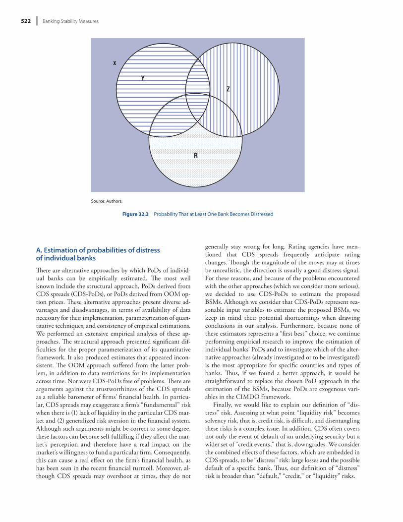
Th e probability that at least one bank becomes distressed (PAO) given that a specifi c bank becomes distressed charac-terizes the likelihood that one, two, or more institutions, up to the total number of banks in the system, become dis-tressed. Th erefore, this mea sure quantifi es the potential “cas-cade” eff ects in the system given distress in a specifi c bank. Consequently, we propose this mea sure as an indicator to quantify the systemic importance of a specifi c bank if it be-comes distressed. Again, it is worth noting that conditional probabilities do not imply causation; however, we consider that the PAO can provide important insights into systemic interlinkages among the banks comprising a system.

For example, in a banking system with four banks, X, Y, Z, and R, the PAO given that Bank X becomes distressed corresponds to the probability set marked in the Venn dia-gram (Figure 32.3). In this example, the PAO can be defi ned as follows:

PAO = P(Y/X ) + P(Z/X ) + P(R/X )P(Y I R/X ) + P(Y I Z/X ) + P(Z I R/X )[ ]

+ P(Y I RI Z/X ). (32.11)

4. BANKING STABILITY MEA SURES: EMPIRICAL RESULTSTo illustrate the methodology, in this section we estimate the proposed BSMs to

1. examine relative changes in stability over time and among diff erent banks’ business;

2. analyze cross- regional eff ects between diff erent bank-ing groups; and

3. analyze the eff ect of foreign banks on sovereigns with banking systems with cross- border institutions.

Our estimations are performed from 2005 up to October 2008 using only publicly available data and include major American and Eu ro pe an banks and sovereigns in Latin America, Eastern Eu rope, and Asia. Implementation fl exi-bility in our approach is of relevance for banking stability surveillance, because cross- border fi nancial linkages are grow-ing and becoming increasingly signifi cant, as has been high-lighted by the fi nancial market turmoil of recent years. Th us, surveillance of banking stability cannot stop at national bor-ders. An important feature of this methodology is that it can be implemented with alternative mea sures of PoDs of indi-vidual banks, which we will describe. We continue by pre-senting the estimated BSMs and analyzing them.

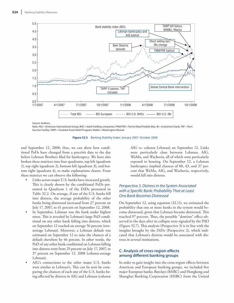
Banking Stability Index

Th e BSI is based on the conditional expectation of the de-fault probability mea sure developed by Huang (1992).17 Th e BSI refl ects the expected number of banks becoming dis-tressed given that at least one bank has become distressed. A higher number signifi es increased instability.

For example, for a system of two banks, the BSI is de-fi ned as follows:

BSI =

P(X xdx ) + P(Y xdy )

1 P(X < xdx , Y < xdy )

.

(32.9)

Th e BSI represents a probability mea sure that conditions on any bank becoming distressed, without indicating the spe-cifi c bank.18

B. Distress between specifi c banks

Distress Dependence Matrix

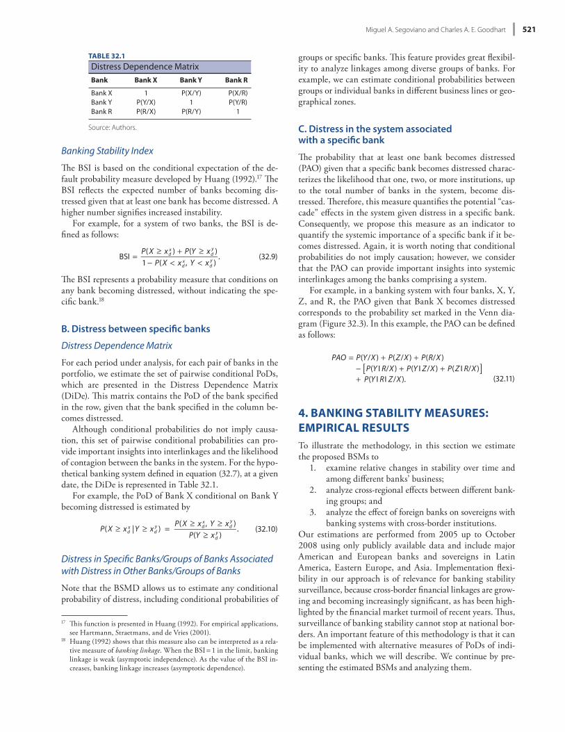
For each period under analysis, for each pair of banks in the portfolio, we estimate the set of pairwise conditional PoDs, which are presented in the Distress Dependence Matrix (DiDe). Th is matrix contains the PoD of the bank specifi ed in the row, given that the bank specifi ed in the column be-comes distressed.

Although conditional probabilities do not imply causa-tion, this set of pairwise conditional probabilities can pro-vide important insights into interlinkages and the likelihood of contagion between the banks in the system. For the hypo-thetical banking system defi ned in equation (32.7), at a given date, the DiDe is represented in Table 32.1.

For example, the PoD of Bank X conditional on Bank Y becoming distressed is estimated by

P(X xdx |Y xd

y ) =P(X xdx , Y xd

y )P(Y xd

y ).

(32.10)

Distress in Specifi c Banks/Groups of Banks Associated with Distress in Other Banks/Groups of Banks

Note that the BSMD allows us to estimate any conditional probability of distress, including conditional probabilities of

17 Th is function is presented in Huang (1992). For empirical applications, see Hartmann, Straetmans, and de Vries (2001).

18 Huang (1992) shows that this mea sure also can be interpreted as a rela-tive mea sure of banking linkage. When the BSI = 1 in the limit, banking linkage is weak (asymptotic in de pen dence). As the value of the BSI in-creases, banking linkage increases (asymptotic dependence).

TABLE 32.1

Distress Dependence MatrixBank Bank X Bank Y Bank R

Bank X 1 P(X/Y) P(X/R)Bank Y P(Y/X) 1 P(Y/R)Bank R P(R/X) P(R/Y) 1

Source: Authors.



generally stay wrong for long. Rating agencies have men-tioned that CDS spreads frequently anticipate rating changes. Th ough the magnitude of the moves may at times be unrealistic, the direction is usually a good distress signal. For these reasons, and because of the problems encountered with the other approaches (which we consider more serious), we decided to use CDS- PoDs to estimate the proposed BSMs. Although we consider that CDS- PoDs represent rea-sonable input variables to estimate the proposed BSMs, we keep in mind their potential shortcomings when drawing conclusions in our analysis. Furthermore, because none of these estimators represents a “fi rst best” choice, we continue performing empirical research to improve the estimation of individual banks’ PoDs and to investigate which of the alter-native approaches (already investigated or to be investigated) is the most appropriate for specifi c countries and types of banks. Th us, if we found a better approach, it would be straightforward to replace the chosen PoD approach in the estimation of the BSMs, because PoDs are exogenous vari-ables in the CIMDO framework.

Finally, we would like to explain our defi nition of “dis-tress” risk. Assessing at what point “liquidity risk” becomes solvency risk, that is, credit risk, is diffi cult, and disentangling these risks is a complex issue. In addition, CDS often covers not only the event of default of an underlying security but a wider set of “credit events,” that is, downgrades. We consider the combined eff ects of these factors, which are embedded in CDS spreads, to be “distress” risk: large losses and the possible default of a specifi c bank. Th us, our defi nition of “distress” risk is broader than “default,” “credit,” or “liquidity” risks.

A. Estimation of probabilities of distress of individual banks

Th ere are alternative approaches by which PoDs of individ-ual banks can be empirically estimated. Th e most well known include the structural approach, PoDs derived from CDS spreads (CDS- PoDs), or PoDs derived from OOM op-tion prices. Th ese alternative approaches present diverse ad-vantages and disadvantages, in terms of availability of data necessary for their implementation, pa ram e terization of quan-titative techniques, and consistency of empirical estimations. We performed an extensive empirical analysis of these ap-proaches. Th e structural approach presented signifi cant dif-fi culties for the proper pa ram e terization of its quantitative framework. It also produced estimates that appeared incon-sistent. Th e OOM approach suff ered from the latter prob-lem, in addition to data restrictions for its implementation across time. Nor were CDS- PoDs free of problems. Th ere are arguments against the trustworthiness of the CDS spreads as a reliable barometer of fi rms’ fi nancial health. In par tic u-lar, CDS spreads may exaggerate a fi rm’s “fundamental” risk when there is (1) lack of liquidity in the par tic u lar CDS mar-ket and (2) generalized risk aversion in the fi nancial system. Although such arguments might be correct to some degree, these factors can become self- fulfi lling if they aff ect the mar-ket’s perception and therefore have a real impact on the market’s willingness to fund a par tic u lar fi rm. Consequently, this can cause a real eff ect on the fi rm’s fi nancial health, as has been seen in the recent fi nancial turmoil. Moreover, al-though CDS spreads may overshoot at times, they do not

x

Y

R

Z

Source: Authors.

Figure 32.3 Probability That at Least One Bank Becomes Distressed



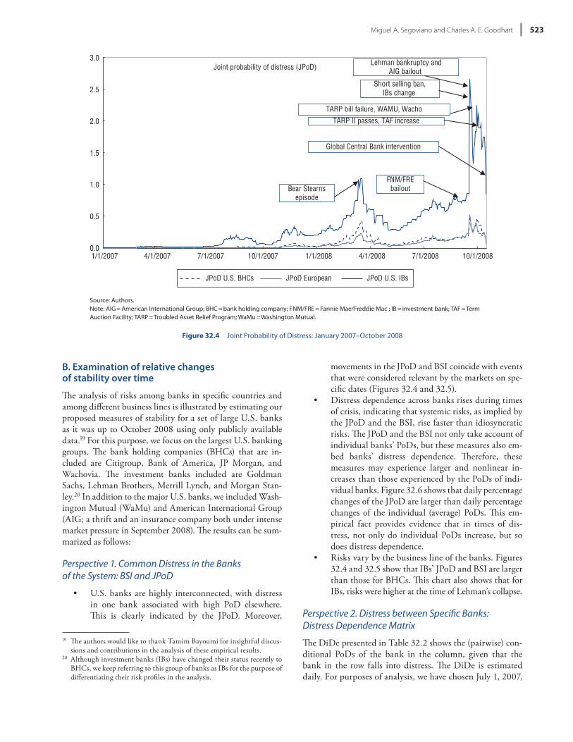
movements in the JPoD and BSI coincide with events that were considered relevant by the markets on spe-cifi c dates (Figures 32.4 and 32.5).

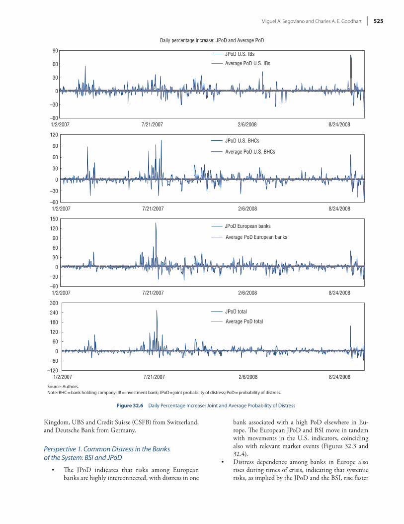
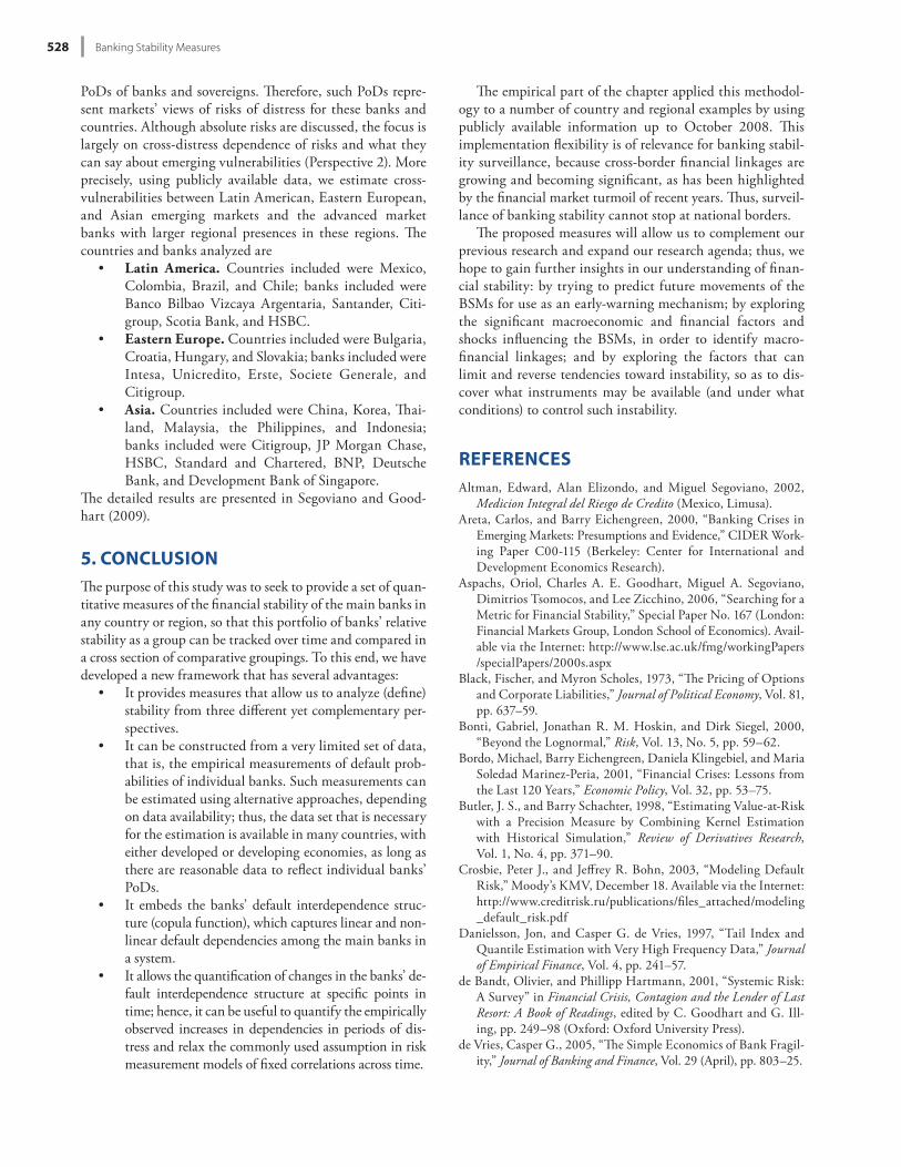
• Distress dependence across banks rises during times of crisis, indicating that systemic risks, as implied by the JPoD and the BSI, rise faster than idiosyncratic risks. Th e JPoD and the BSI not only take account of individual banks’ PoDs, but these mea sures also em-bed banks’ distress dependence. Th erefore, these mea sures may experience larger and nonlinear in-creases than those experienced by the PoDs of indi-vidual banks. Figure 32.6 shows that daily percentage changes of the JPoD are larger than daily percentage changes of the individual (average) PoDs. Th is em-pirical fact provides evidence that in times of dis-tress, not only do individual PoDs increase, but so does distress dependence.

• Risks vary by the business line of the banks. Figures 32.4 and 32.5 show that IBs’ JPoD and BSI are larger than those for BHCs. Th is chart also shows that for IBs, risks were higher at the time of Lehman’s collapse.

Perspective 2. Distress between Specifi c Banks: Distress Dependence Matrix

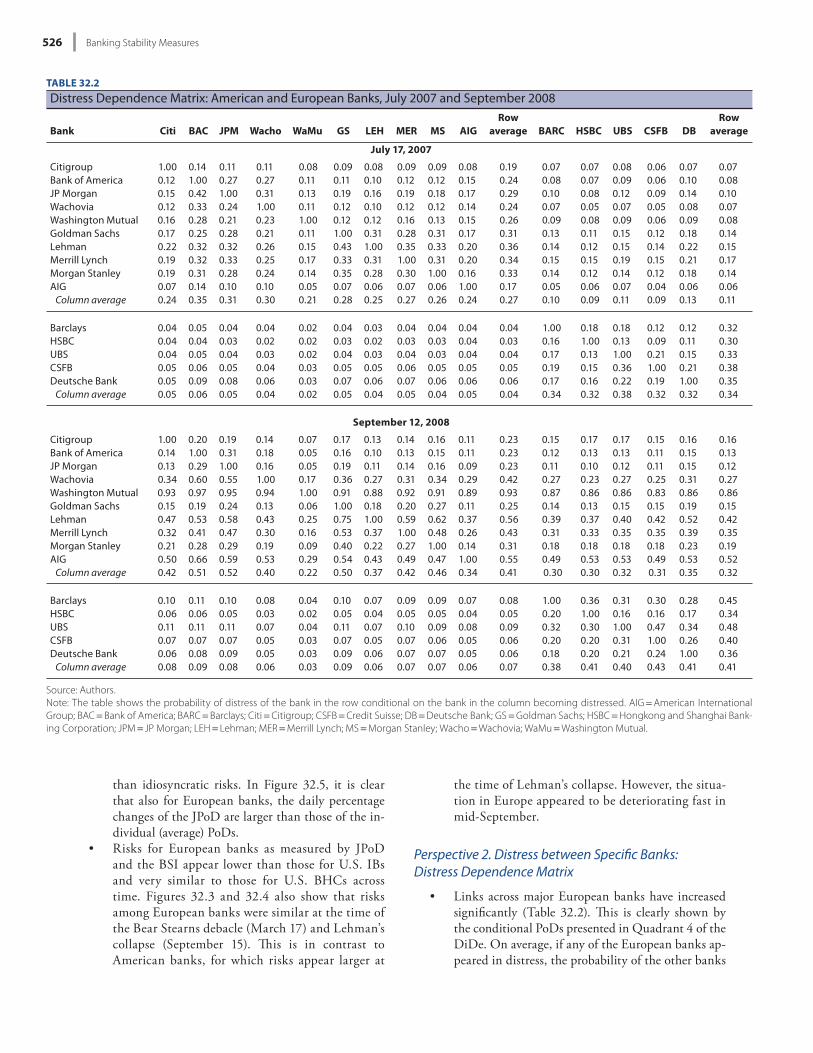
Th e DiDe presented in Table 32.2 shows the (pairwise) con-ditional PoDs of the bank in the column, given that the bank in the row falls into distress. Th e DiDe is estimated daily. For purposes of analysis, we have chosen July 1, 2007,

B. Examination of relative changes of stability over time

Th e analysis of risks among banks in specifi c countries and among diff erent business lines is illustrated by estimating our proposed mea sures of stability for a set of large U.S. banks as it was up to October 2008 using only publicly available data.19 For this purpose, we focus on the largest U.S. banking groups. Th e bank holding companies (BHCs) that are in-cluded are Citigroup, Bank of America, JP Morgan, and Wachovia. Th e investment banks included are Goldman Sachs, Lehman Brothers, Merrill Lynch, and Morgan Stan-ley.20 In addition to the major U.S. banks, we included Wash-ington Mutual (WaMu) and American International Group (AIG; a thrift and an insurance company both under intense market pressure in September 2008). Th e results can be sum-marized as follows:

Perspective 1. Common Distress in the Banks of the System: BSI and JPoD

• U.S. banks are highly interconnected, with distress in one bank associated with high PoD elsewhere. Th is is clearly indicated by the JPoD. Moreover,

19 Th e authors would like to thank Tamim Bayoumi for insightful discus-sions and contributions in the analysis of these empirical results.

20 Although investment banks (IBs) have changed their status recently to BHCs, we keep referring to this group of banks as IBs for the purpose of diff erentiating their risk profi les in the analysis.

0.0

0.5

1.0

1.5

2.0

2.5

3.0

1/1/2007 4/1/2007 7/1/2007 10/1/2007 1/1/2008 4/1/2008 7/1/2008 10/1/2008

Joint probability of distress (JPoD)

FNM/FREbailoutBear Stearns

episode

Lehman bankruptcy andAIG bailout

TARP bill failure, WAMU, Wacho

Short selling ban, IBs change

TARP II passes, TAF increase

Global Central Bank intervention

JPoD U.S. BHCs JPoD European JPoD U.S. IBs

Source: Authors.Note: AIG = American International Group; BHC = bank holding company; FNM/FRE = Fannie Mae/Freddie Mac ; IB = investment bank; TAF = Term Auction Facility; TARP = Troubled Asset Relief Program; WaMu = Washington Mutual.

Figure 32.4 Joint Probability of Distress: January 2007– October 2008



AIG vs. column Lehman) on September 12. Links were particularly close between Lehman, AIG, WaMu, and Wachovia, all of which were particularly exposed to housing. On September 12, a Lehman bankruptcy implied chances of 88, 43, and 27 per-cent that WaMu, AIG, and Wachovia, respectively, would fall into distress.

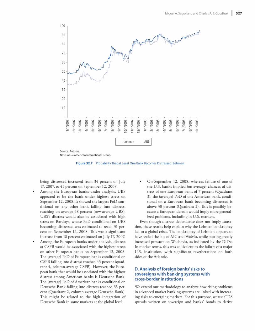
Perspective 3. Distress in the System Associated with a Specifi c Bank: Probability That at Least One Bank Becomes Distressed

On September 12, using equation (32.11), we estimated the probability that one or more banks in the system would be-come distressed, given that Lehman became distressed. Th is reached 97 percent. Th us, the possible “domino” eff ect ob-served in the days after its collapse were signaled by the PAO (Figure 32.7). Th is analysis (Perspective 3) is in line with the insights brought by the DiDe (Perspective 2), which indi-cated that Lehman’s distress would be associated with dis-tress in several institutions.

C. Analysis of cross- region eff ects among diff erent banking groups

In order to gain insight into the cross- region eff ects between American and Eu ro pe an banking groups, we included fi ve major Eu ro pe an banks: Barclays (BARC) and Hongkong and Shanghai Banking Corporation (HSBC) from the United

and September 12, 2008; thus, we can show how condi-tional PoDs have changed from a precrisis date to the day before Lehman Brothers fi led for bankruptcy. We have also broken these matrices into four quadrants, top left (quadrant 1), top right (quadrant 2), bottom left (quadrant 3), and bot-tom right (quadrant 4), to make explanations clearer. From these matrices we can observe the following:

• Links across major U.S. banks have increased greatly. Th is is clearly shown by the conditional PoDs pre-sented in Quadrant 1 of the DiDe presented in Table 32.2. On average, if any of the U.S. banks fell into distress, the average probability of the other banks being distressed increased from 27 percent on July 17, 2007, to 41 percent on September 12, 2008.

• In September, Lehman was the bank under highest stress. Th is is revealed by Lehman’s large PoD condi-tional on any other bank falling into distress, which on September 12 reached on average 56 percent (row- average Lehman). Moreover, a Lehman default was estimated on September 12 to raise the chances of a default elsewhere by 46 percent. In other words, the PoD of any other bank conditional on Lehman falling into distress went from 25 percent on July 17, 2007, to 37 percent on September 12, 2008 (column- average Lehman).

• AIG’s connections to the other major U.S. banks were similar to Lehman’s. Th is can be seen by com-paring the chances of each one of the U.S. banks be-ing aff ected by distress in AIG and Lehman (column

0.0

0.5

1.0

1.5

2.0

2.5

3.0

3.5

4.0

4.5

5.0

1/1/2007 4/1/2007 7/1/2007 10/1/2007 1/1/2008 4/1/2008 7/1/2008 10/1/2008

Bank stability index (BSI)

FNM/FRE bailout

Bear Stearnsepisode

Lehman bankruptcy andAIG bailout

TARP bill failure,WAMU, Wacho

Short selling ban, IBs change

TARP II passes, TAFincrease

Global Central Bank intervention

Total BSI BSI European BSI U.S. BHCs BSI U.S. IBs

Source: Authors.Note: AIG = American International Group; BHC = bank holding companies; FNM/FRE = Fannie Mae/Freddie Mac; IB = investment bank; TAF = Term Auction Facility; TARP = Troubled Asset Relief Program; WaMu = Washington Mutual.

Figure 32.5 Banking Stability Index: January 2007– October 2008



bank associated with a high PoD elsewhere in Eu-rope. Th e Eu ro pe an JPoD and BSI move in tandem with movements in the U.S. indicators, coinciding also with relevant market events (Figures 32.3 and 32.4).

• Distress dependence among banks in Eu rope also rises during times of crisis, indicating that systemic risks, as implied by the JPoD and the BSI, rise faster

Kingdom, UBS and Credit Suisse (CSFB) from Switzerland, and Deutsche Bank from Germany.

Perspective 1. Common Distress in the Banks of the System: BSI and JPoD

• Th e JPoD indicates that risks among Eu ro pe an banks are highly interconnected, with distress in one

Daily percentage increase: JPoD and Average PoD

–60

–30

0

30

60

90

1/2/2007 7/21/2007 2/6/2008 8/24/2008

JPoD U.S. IBs

Average PoD U.S. IBs

–60

–30

0

30

60

90

120

1/2/2007 7/21/2007 2/6/2008 8/24/2008

JPoD U.S. BHCs

Average PoD U.S. BHCs

–60

–30

0

30

60

90

120

150

1/2/2007 7/21/2007 2/6/2008 8/24/2008

JPoD European banks

Average PoD European banks

–120

–60

0

60

120

180

240

300

1/2/2007 7/21/2007 2/6/2008 8/24/2008

JPoD total

Average PoD total

Source: Authors.Note: BHC = bank holding company; IB = investment bank; JPoD = joint probability of distress; PoD = probability of distress.

Figure 32.6 Daily Percentage Increase: Joint and Average Probability of Distress



the time of Lehman’s collapse. However, the situa-tion in Eu rope appeared to be deteriorating fast in mid- September.

Perspective 2. Distress between Specifi c Banks: Distress Dependence Matrix

• Links across major Eu ro pe an banks have increased signifi cantly (Table 32.2). Th is is clearly shown by the conditional PoDs presented in Quadrant 4 of the DiDe. On average, if any of the Eu ro pe an banks ap-peared in distress, the probability of the other banks

than idiosyncratic risks. In Figure 32.5, it is clear that also for Eu ro pe an banks, the daily percentage changes of the JPoD are larger than those of the in-dividual (average) PoDs.

• Risks for Eu ro pe an banks as mea sured by JPoD and the BSI appear lower than those for U.S. IBs and very similar to those for U.S. BHCs across time. Figures 32.3 and 32.4 also show that risks among Eu ro pe an banks were similar at the time of the Bear Stearns debacle (March 17) and Lehman’s collapse (September 15). Th is is in contrast to American banks, for which risks appear larger at

TABLE 32.2

Distress Dependence Matrix: American and Eu ro pe an Banks, July 2007 and September 2008

Bank Citi BAC JPM Wacho WaMu GS LEH MER MS AIGRow

average BARC HSBC UBS CSFB DBRow

average

July 17, 2007

Citigroup 1.00 0.14 0.11 0.11 0.08 0.09 0.08 0.09 0.09 0.08 0.19 0.07 0.07 0.08 0.06 0.07 0.07Bank of America 0.12 1.00 0.27 0.27 0.11 0.11 0.10 0.12 0.12 0.15 0.24 0.08 0.07 0.09 0.06 0.10 0.08JP Morgan 0.15 0.42 1.00 0.31 0.13 0.19 0.16 0.19 0.18 0.17 0.29 0.10 0.08 0.12 0.09 0.14 0.10Wachovia 0.12 0.33 0.24 1.00 0.11 0.12 0.10 0.12 0.12 0.14 0.24 0.07 0.05 0.07 0.05 0.08 0.07Washington Mutual 0.16 0.28 0.21 0.23 1.00 0.12 0.12 0.16 0.13 0.15 0.26 0.09 0.08 0.09 0.06 0.09 0.08Goldman Sachs 0.17 0.25 0.28 0.21 0.11 1.00 0.31 0.28 0.31 0.17 0.31 0.13 0.11 0.15 0.12 0.18 0.14Lehman 0.22 0.32 0.32 0.26 0.15 0.43 1.00 0.35 0.33 0.20 0.36 0.14 0.12 0.15 0.14 0.22 0.15Merrill Lynch 0.19 0.32 0.33 0.25 0.17 0.33 0.31 1.00 0.31 0.20 0.34 0.15 0.15 0.19 0.15 0.21 0.17Morgan Stanley 0.19 0.31 0.28 0.24 0.14 0.35 0.28 0.30 1.00 0.16 0.33 0.14 0.12 0.14 0.12 0.18 0.14AIG 0.07 0.14 0.10 0.10 0.05 0.07 0.06 0.07 0.06 1.00 0.17 0.05 0.06 0.07 0.04 0.06 0.06 Column average 0.24 0.35 0.31 0.30 0.21 0.28 0.25 0.27 0.26 0.24 0.27 0.10 0.09 0.11 0.09 0.13 0.11

Barclays 0.04 0.05 0.04 0.04 0.02 0.04 0.03 0.04 0.04 0.04 0.04 1.00 0.18 0.18 0.12 0.12 0.32HSBC 0.04 0.04 0.03 0.02 0.02 0.03 0.02 0.03 0.03 0.04 0.03 0.16 1.00 0.13 0.09 0.11 0.30UBS 0.04 0.05 0.04 0.03 0.02 0.04 0.03 0.04 0.03 0.04 0.04 0.17 0.13 1.00 0.21 0.15 0.33CSFB 0.05 0.06 0.05 0.04 0.03 0.05 0.05 0.06 0.05 0.05 0.05 0.19 0.15 0.36 1.00 0.21 0.38Deutsche Bank 0.05 0.09 0.08 0.06 0.03 0.07 0.06 0.07 0.06 0.06 0.06 0.17 0.16 0.22 0.19 1.00 0.35 Column average 0.05 0.06 0.05 0.04 0.02 0.05 0.04 0.05 0.04 0.05 0.04 0.34 0.32 0.38 0.32 0.32 0.34

September 12, 2008

Citigroup 1.00 0.20 0.19 0.14 0.07 0.17 0.13 0.14 0.16 0.11 0.23 0.15 0.17 0.17 0.15 0.16 0.16Bank of America 0.14 1.00 0.31 0.18 0.05 0.16 0.10 0.13 0.15 0.11 0.23 0.12 0.13 0.13 0.11 0.15 0.13JP Morgan 0.13 0.29 1.00 0.16 0.05 0.19 0.11 0.14 0.16 0.09 0.23 0.11 0.10 0.12 0.11 0.15 0.12Wachovia 0.34 0.60 0.55 1.00 0.17 0.36 0.27 0.31 0.34 0.29 0.42 0.27 0.23 0.27 0.25 0.31 0.27Washington Mutual 0.93 0.97 0.95 0.94 1.00 0.91 0.88 0.92 0.91 0.89 0.93 0.87 0.86 0.86 0.83 0.86 0.86Goldman Sachs 0.15 0.19 0.24 0.13 0.06 1.00 0.18 0.20 0.27 0.11 0.25 0.14 0.13 0.15 0.15 0.19 0.15Lehman 0.47 0.53 0.58 0.43 0.25 0.75 1.00 0.59 0.62 0.37 0.56 0.39 0.37 0.40 0.42 0.52 0.42Merrill Lynch 0.32 0.41 0.47 0.30 0.16 0.53 0.37 1.00 0.48 0.26 0.43 0.31 0.33 0.35 0.35 0.39 0.35Morgan Stanley 0.21 0.28 0.29 0.19 0.09 0.40 0.22 0.27 1.00 0.14 0.31 0.18 0.18 0.18 0.18 0.23 0.19AIG 0.50 0.66 0.59 0.53 0.29 0.54 0.43 0.49 0.47 1.00 0.55 0.49 0.53 0.53 0.49 0.53 0.52 Column average 0.42 0.51 0.52 0.40 0.22 0.50 0.37 0.42 0.46 0.34 0.41 0.30 0.30 0.32 0.31 0.35 0.32

Barclays 0.10 0.11 0.10 0.08 0.04 0.10 0.07 0.09 0.09 0.07 0.08 1.00 0.36 0.31 0.30 0.28 0.45HSBC 0.06 0.06 0.05 0.03 0.02 0.05 0.04 0.05 0.05 0.04 0.05 0.20 1.00 0.16 0.16 0.17 0.34UBS 0.11 0.11 0.11 0.07 0.04 0.11 0.07 0.10 0.09 0.08 0.09 0.32 0.30 1.00 0.47 0.34 0.48CSFB 0.07 0.07 0.07 0.05 0.03 0.07 0.05 0.07 0.06 0.05 0.06 0.20 0.20 0.31 1.00 0.26 0.40Deutsche Bank 0.06 0.08 0.09 0.05 0.03 0.09 0.06 0.07 0.07 0.05 0.06 0.18 0.20 0.21 0.24 1.00 0.36 Column average 0.08 0.09 0.08 0.06 0.03 0.09 0.06 0.07 0.07 0.06 0.07 0.38 0.41 0.40 0.43 0.41 0.41

Source: Authors.Note: The table shows the probability of distress of the bank in the row conditional on the bank in the column becoming distressed. AIG = American International Group; BAC = Bank of America; BARC = Barclays; Citi = Citigroup; CSFB = Credit Suisse; DB = Deutsche Bank; GS = Goldman Sachs; HSBC = Hongkong and Shanghai Bank-ing Corporation; JPM = JP Morgan; LEH = Lehman; MER = Merrill Lynch; MS = Morgan Stanley; Wacho = Wachovia; WaMu = Washington Mutual.



• On September 12, 2008, whereas failure of one of the U.S. banks implied (on average) chances of dis-tress of one Eu ro pe an bank of 7 percent (Quadrant 3), the (average) PoD of one American bank, condi-tional on a Eu ro pe an bank becoming distressed is above 30 percent (Quadrant 2). Th is is possibly be-cause a Eu ro pe an default would imply more general-ized problems, including in U.S. markets.

Even though distress dependence does not imply causa-tion, these results help explain why the Lehman bankruptcy led to a global crisis. Th e bankruptcy of Lehman appears to have sealed the fate of AIG and WaMu, while putting greatly increased pressure on Wachovia, as indicated by the DiDe. In market terms, this was equivalent to the failure of a major U.S. institution, with signifi cant reverberations on both sides of the Atlantic.

D. Analysis of foreign banks’ risks to sovereigns with banking systems with cross- border institutions

We extend our methodology to analyze how rising problems in advanced market banking systems are linked with increas-ing risks to emerging markets. For this purpose, we use CDS spreads written on sovereign and banks’ bonds to derive

being distressed increased from 34 percent on July 17, 2007, to 41 percent on September 12, 2008.

• Among the Eu ro pe an banks under analysis, UBS appeared to be the bank under highest stress on September 12, 2008. It showed the largest PoD con-ditional on any other bank falling into distress, reaching on average 48 percent (row- average UBS). UBS’s distress would also be associated with high stress on Barclays, whose PoD conditional on UBS becoming distressed was estimated to reach 31 per-cent on September 12, 2008. Th is was a signifi cant increase from 18 percent estimated on July 17, 2007.

• Among the Eu ro pe an banks under analysis, distress at CSFB would be associated with the highest stress on other Eu ro pe an banks on September 12, 2008. Th e (average) PoD of Eu ro pe an banks conditional on CSFB falling into distress reached 43 percent (quad-rant 4, column- average CSFB). However, the Eu ro-pe an bank that would be associated with the highest distress among American banks is Deutsche Bank. Th e (average) PoD of American banks conditional on Deutsche Bank falling into distress reached 35 per-cent (Quadrant 2, column- average Deutsche Bank). Th is might be related to the high integration of Deutsche Bank in some markets at the global level.

0

10

20

30

40

50

60

70

80

90

100

1/1/

2007

2/1/

2007

3/1/

2007

4/1/

2007

5/1/

2007

6/1/

2007

7/1/

2007

8/1/

2007

9/1/

2007

10/1

/200

7

11/1

/200

7

12/1

/200

7

1/1/

2008

2/1/

2008

3/1/

2008

4/1/

2008

5/1/

2008

6/1/

2008

7/1/

2008

8/1/

2008

9/1/

2008

Lehman AIG

Source: Authors.Note: AIG = American International Group.

Figure 32.7 Probability That at Least One Bank Becomes Distressed: Lehman



Th e empirical part of the chapter applied this methodol-ogy to a number of country and regional examples by using publicly available information up to October 2008. Th is implementation fl exibility is of relevance for banking stabil-ity surveillance, because cross- border fi nancial linkages are growing and becoming signifi cant, as has been highlighted by the fi nancial market turmoil of recent years. Th us, surveil-lance of banking stability cannot stop at national borders.

Th e proposed mea sures will allow us to complement our previous research and expand our research agenda; thus, we hope to gain further insights in our understanding of fi nan-cial stability: by trying to predict future movements of the BSMs for use as an early- warning mechanism; by exploring the signifi cant macroeconomic and fi nancial factors and shocks infl uencing the BSMs, in order to identify macro- fi nancial linkages; and by exploring the factors that can limit and reverse tendencies toward instability, so as to dis-cover what instruments may be available (and under what conditions) to control such instability.

REFERENCESAltman, Edward, Alan Elizondo, and Miguel Segoviano, 2002,

Medicion Integral del Riesgo de Credito (Mexico, Limusa).Areta, Carlos, and Barry Eichengreen, 2000, “Banking Crises in

Emerging Markets: Presumptions and Evidence,” CIDER Work-ing Paper C00- 115 (Berkeley: Center for International and Development Economics Research).

Aspachs, Oriol, Charles A. E. Goodhart, Miguel A. Segoviano, Dimitrios Tsomocos, and Lee Zicchino, 2006, “Searching for a Metric for Financial Stability,” Special Paper No. 167 (London: Financial Markets Group, London School of Economics). Avail-able via the Internet: http:// www .lse .ac .uk /fmg /workingPapers /specialPapers /2000s .aspx

Black, Fischer, and Myron Scholes, 1973, “Th e Pricing of Options and Corporate Liabilities,” Journal of Po liti cal Economy, Vol. 81, pp. 637– 59.

Bonti, Gabriel, Jonathan R. M. Hoskin, and Dirk Siegel, 2000, “Beyond the Lognormal,” Risk, Vol. 13, No. 5, pp. 59– 62.

Bordo, Michael, Barry Eichengreen, Daniela Klingebiel, and Maria Soledad Marinez- Peria, 2001, “Financial Crises: Lessons from the Last 120 Years,” Economic Policy, Vol. 32, pp. 53– 75.

Butler, J. S., and Barry Schachter, 1998, “Estimating Value- at- Risk with a Precision Mea sure by Combining Kernel Estimation with Historical Simulation,” Review of Derivatives Research, Vol. 1, No. 4, pp. 371– 90.

Crosbie, Peter J., and Jeff rey R. Bohn, 2003, “Modeling Default Risk,” Moody’s KMV, December 18. Available via the Internet: http:// www .creditrisk .ru /publications /fi les _attached /modeling _default _risk .pdf

Danielsson, Jon, and Casper G. de Vries, 1997, “Tail Index and Quantile Estimation with Very High Frequency Data,” Journal of Empirical Finance, Vol. 4, pp. 241– 57.

de Bandt, Olivier, and Phillipp Hartmann, 2001, “Systemic Risk: A Survey” in Financial Crisis, Contagion and the Lender of Last Resort: A Book of Readings, edited by C. Goodhart and G. Ill-ing, pp. 249– 98 (Oxford: Oxford University Press).

de Vries, Casper G., 2005, “Th e Simple Economics of Bank Fragil-ity,” Journal of Banking and Finance, Vol. 29 (April), pp. 803– 25.

PoDs of banks and sovereigns. Th erefore, such PoDs repre-sent markets’ views of risks of distress for these banks and countries. Although absolute risks are discussed, the focus is largely on cross- distress dependence of risks and what they can say about emerging vulnerabilities (Perspective 2). More precisely, using publicly available data, we estimate cross- vulnerabilities between Latin American, Eastern Eu ro pe an, and Asian emerging markets and the advanced market banks with larger regional presences in these regions. Th e countries and banks analyzed are

• Latin America. Countries included were Mexico, Colombia, Brazil, and Chile; banks included were Banco Bilbao Vizcaya Argentaria, Santander, Citi-group, Scotia Bank, and HSBC.

• Eastern Eu rope. Countries included were Bulgaria, Croatia, Hungary, and Slovakia; banks included were Intesa, Unicredito, Erste, Societe Generale, and Citigroup.

• Asia. Countries included were China, Korea, Th ai-land, Malaysia, the Philippines, and Indonesia; banks included were Citigroup, JP Morgan Chase, HSBC, Standard and Chartered, BNP, Deutsche Bank, and Development Bank of Singapore.

Th e detailed results are presented in Segoviano and Good-hart (2009).

5. CONCLUSIONTh e purpose of this study was to seek to provide a set of quan-titative mea sures of the fi nancial stability of the main banks in any country or region, so that this portfolio of banks’ relative stability as a group can be tracked over time and compared in a cross section of comparative groupings. To this end, we have developed a new framework that has several advantages:

• It provides mea sures that allow us to analyze (defi ne) stability from three diff erent yet complementary per-spectives.

• It can be constructed from a very limited set of data, that is, the empirical mea sure ments of default prob-abilities of individual banks. Such mea sure ments can be estimated using alternative approaches, depending on data availability; thus, the data set that is necessary for the estimation is available in many countries, with either developed or developing economies, as long as there are reasonable data to refl ect individual banks’ PoDs.

• It embeds the banks’ default interdependence struc-ture (copula function), which captures linear and non-linear default dependencies among the main banks in a system.

• It allows the quantifi cation of changes in the banks’ de-fault interdependence structure at specifi c points in time; hence, it can be useful to quantify the empirically observed increases in dependencies in periods of dis-tress and relax the commonly used assumption in risk mea sure ment models of fi xed correlations across time.



———, 1984, “Prior Information and Ambiguity in Inverse Prob-lems,” in Inverse Problems, SIAM- AMS Proceedings, edited by D. W. McLaughlin, Vol. 14, pp. 151– 66 (Providence: Ameri-can Mathematical Society).

Kaminsky, Graciela, and Carmen Reinhart, 1999, “Th e Twin Crisis: Th e Causes of Banking and Balance of Payments Problems,” American Economic Review, Vol. 89, No. 3, pp. 473– 500.

Kiyotaki, Nobuhiro, and John Moore, 1997, “Credit Cycles,” Jour-nal of Po liti cal Economy, Vol. 105, No. 2, pp. 211– 48.

Krugman, Paul, 1979, “A Model of Balance of Payments Crises,” Journal of Money, Credit and Banking, Vol. 11, No. 3, pp. 311– 25.

Kullback, S., 1959, Information Th eory and Statistics (New York: John Wiley).

———, and R. Leibler, 1951, “On Information and Suffi ciency,” Annals of Mathematical Statistics, Vol. 22, No. 1, pp. 79– 86.

Merton, Robert C., 1974, “On the Pricing of Corporate Debt: Th e Risk Structure of Interest Rates,” Journal of Finance, Vol. 29, No. 2, pp. 449– 70.

Nelsen, Roger B., 1999, “An Introduction to Copulas,” Lecture Notes Statistics, 2nd Edition, Vol. 139.

Segoviano, Miguel A., 1998, “A Structural Approach for Portfolio Credit Risk vs. Creditmetrics” (unpublished; London: London School of Economics).

———, 2004, “A System for Mea sur ing Credit Risk When Only Limited Data Is Available,” Credit Risk International, London, October 2004.

———, 2006a, “Th e Conditional Probability of Default Method-ology,” Discussion Paper No. 558 (London: Financial Markets Group, London School of Economics). Available via the Inter-net: http:// eprints .lse .ac .uk /24512 /

———, 2006b, “Th e Consistent Information Multivariate Density Optimizing Methodology,” Discussion Paper No. 557 (London: Financial Markets Group, London School of Economics). Avail-able via the Internet: http:// eprints .lse .ac .uk /24511 /

———, and Charles A. E. Goodhart, 2009, “Banking Stability Mea sures,” Working Paper 09/4 (Washington: International Monetary Fund). Available via the Internet: http:// www .imf .org /external /pubs /cat /longres .aspx ?sk=22554 .0

Segoviano, Miguel A., and Philip Lowe, 2002, “Internal Ratings, the Business Cycle and Capital Requirements: Some Evidence from an Emerging Market Economy,” BIS Working Paper No. 117 (Basel: Bank for International Settlements). Available via the Internet: http:// www .bis .org /publ /work117 .htm

Segoviano, Miguel A., and Pablo Padilla, 2006, “Portfolio Credit Risk and Macroeconomic Shocks: Applications to Stress Testing under Data Restricted Environments,” Working Paper 06/283 (Washington: International Monetary Fund). Available via the Internet: http:// www .imf .org /external /pubs /cat /lon-gres .aspx ?sk=19902 .0

Sklar, Abe, 1959, “Fonctions de répartition d n dimensions et leurs marges,” Publications de l’Institut de Statistique de l’Univiversité de Paris, Vol. 8, pp. 229–31.

Diebold, Francis X., Jin Hahn, and Anthony S. Tay, 1999, “Multi-variate Density Forecast Evaluation and Calibration in Finan-cial Risk Management: High- Frequency Returns on Foreign Exchange,” Review of Economics and Statistics, Vol. 81, No. 4, pp. 661– 73.

Embrechts, Paul, Alexander J. McNeil, and Daniel Straumann, 1999, “Correlation and Dependence Properties in Risk Man-agement: Properties and Pitfalls,” Working Paper (Zu rich: ETH Zu rich, RiskLab).

Frey, Rudiger., and Alexander J. McNeil, 2001, “Modelling Dependent Defaults,” Working Paper (Zu rich: ETH Zu rich, Department of Mathematics).

Glasserman, Paul, Philip Heidelberger, and Perwez Shahabuddin, 2002, “Portfolio Value- at- Risk with Heavy- Tailed Risk Fac-tors,” Mathematical Finance, Vol. 12, No. 3, pp. 239– 69.

Golan, Amos, and George G. Judge, 1992, “Recovering Informa-tion in the Case of Ill- Posed Inverse Problems with Noise,” mimeo (Berkeley: University of California, Berkeley).

Goodhart, Charles, 1995, “Price Stability and Financial Fragility,” in Financial Stability in a Changing Environment, edited by K. Sawamoto, Z. Nakajima, and H. Taguchi (New York: St. Martin’s Press).

———, and Boris Hofmann, 2003, “Defl ation, Credit, and Asset Prices,” in Th e Anatomy of Defl ation, edited by Pierre Siklos and Richard Burdekin (Cambridge: Cambridge University Press).

———, and Miguel A. Segoviano, 2004, “Bank Regulation and Macroeconomic Fluctuations,” Oxford Review of Economic Policy, Vol. 20, No. 4, pp. 591– 615.

———, 2006, “Default, Credit Growth, and Asset Prices,” IMF Working Paper 06/223 (Washington: International Monetary Fund). Available via the Internet: http:// www .imf .org /external /pubs /cat /longres .aspx ?sk=19902 .0

Goodhart, Charles A. E., and Miguel A. Segoviano, 2004, “Basel and Procyclicality: A Comparison of the Standardized and IRB Approaches to an Improved Credit Risk Method,” Discussion Paper No. 524 (London: Financial Markets Group, London School of Economics). Available via the Internet: http:// eprints .lse .ac .uk /24821

Goodhart, Charles A. E., Pojanart Sunirand, and Dimitrios Tsomocos, 2006, “A Model to Analyse Financial Fragility,” Economic Th eory, Vol. 27, No. 1, pp. 107– 42.

Hartmann, P., S. Straetmans, and C. de Vries, 2001, “Asset Mar-ket Linkages in Crisis Periods,” Working Paper No. 71 (Frank-furt: Eu ro pe an Central Bank). Available via the Internet: http:// www .ecb .europa .eu /pub /scientifi c /wps /date /html /wps2001 . en .html

Hoelscher, David S., 2006, Bank Restructuring and Resolution (Washington: International Monetary Fund).

Huang, Xin, 1992, “Statistics of Bivariate Extreme Values” (Ph.D. thesis, No. 22, Tinbergen Institute Research Series; Rotter-dam, the Netherlands: Erasmus University).

Jaynes, Edwin T., 1957, “Information Th eory and Statistical Me-chanics,” Physical Review, Vol. 106, No. 4, pp. 620– 30.



Documents

Banking Stability Mea sures...514 Banking Stability Mea sures cycle.4 Consequently, the proposed BSMs represent a set of tools to analyze (defi ne) stability from four diff erent yet