Bank Productivity and Performance Groups: A Decomposition

Bank Productivity and Performance Groups:

A Decomposition Approach Based

upon the Luenberger Productivity Indicator*

Mircea Epure†

Kristiaan Kerstens‡

Diego Prior§

December 2008, This revision: January 2011

Forthcoming, European Journal of Operational Research, 2011

Abstract The purpose of this paper is twofold. First, in the framework of the strategic groups’ literature, it analyses changes in productivity and efficiency of Spanish private and savings banks over an eight-year period (1998–2006). Second, by adapting the decomposition of the Malmquist productivity indices suggested by Färe et al. (1994), it proposes similar components decomposing the Luenberger productivity indicator. Initially, productivity is decomposed into technological and efficiency changes. Thereafter, this efficiency change is decomposed into pure efficiency, scale and congestion changes. Empirical results demonstrate that productivity improvements are partially due to technological innovation. Furthermore, it is shown how the competition between private and savings banks develops in terms of the analyzed productivity and efficiency components. While private banks enjoy better efficiency change, savings banks contribute more to technological progress. Consequently, the Luenberger components are used as cluster analysis inputs. Thus, economic interpretations of the resulting performance groups are made via key differences in productivity components. Finally, following the strategic groups’ literature, supplementary insights are gained by linking these performance groups with banking ratios. Keywords: Luenberger decomposition, productivity, efficiency, Spanish banking sector, performance groups, banking ratios.

* The authors thank three referees and conference participants at NAPW2008 and ACEDE2008 for constructive comments. The usual disclaimer applies. M. Epure acknowledges the support received from “Commission of Universities and Research of the Innovation Department, Universities and Enterprise of the Catalan Government and the European Social Funds”. D. Prior acknowledges the financial support from the Spanish “Ministerio de Educación y Ciencia” under project ECO2010-18967. † Departament d'Economia de l'Empresa, Universitat Autònoma de Barcelona, Edifici B, E-08193 Bellaterra, [email protected]. ‡ CNRS-LEM (UMR 8179), IESEG School of Management, 3 rue de la Digue, F-59800 Lille, France, [email protected]. § Departament d'Economia de l'Empresa, Universitat Autònoma de Barcelona, Edifici B, E-08193 Bellaterra and IESEG School of Management, [email protected]. Corresponding author.

1

1. Introduction

The purpose of this paper is to analyze the changes in productivity and efficiency

within the Spanish banking sector throughout an eight-year period (1998–2006).

Following the decomposition of the Malmquist productivity indices suggested by Färe

et al. (1994), we propose a novel decomposition of the Luenberger productivity

indicator. Thereafter, we continue by clustering these results to show the significant

dissimilarities between performance groups in a dynamic perspective. Thus, the article

aims at presenting a comprehensive image of the evolution of the competitive reality of

the Spanish banking industry.

The use of primal productivity indices in the academic literature on efficiency and

productivity has recently experienced an upsurge in popularity. This is because these do

not require the availability of prices (information which is not always available), but

rather rely on physical inputs and outputs solely. Numerous empirical applications

employ the ratio-based Malmquist productivity index (see the survey in Färe et al. 1998

or the more recent review in Fethi and Pasiouras 2010). However, fewer applications

are based on the more recent Luenberger productivity indicator (Chambers 2002), which

measures productivity in terms of differences rather than ratios.

Several differences exist between ratio- and difference-based productivity

measures. In index number theory, indicators have been proposed to avoid certain

problems with index calculations (see e.g., Diewert 2005). One source of nuisance for

the ratio-based indices occurs when the denominator yields a zero value.1 Of course,

these issues are less likely to appear in frontier benchmarking. Nevertheless, Chambers

et al. (1996) defined Luenberger productivity indicators to answer these issues. 2

Additionally, there is a more practical consideration in favor of the use of indicators.

Even if the academic community is familiar with ratios, the business and accounting

communities are evidently more accustomed to evaluating cost, revenue, or profit

differences in monetary terms (Boussemart et al. 2003).

Luenberger indicators are more general than Malmquist indices, since these use

proportional distance functions that are compatible with the goal of profit maximization,

1 The issue of zero values in the indices and indicators must be distinguished from the issue of zero inputs and outputs in the data matrices constituting the technology. See Färe et al. (1994: 44-45) for the exact conditions on these data matrices. However, zero inputs or outputs do not pose a problem for computing the proportional distance function in general (see Section 2 for its definition). 2 As Chambers (2002: 756) states, “one of the most common practical problems with ratio-based indexes is what to do with zero observations, as ratio-based indexes are frequently not well defined in the neighborhood of the origin.”

2

while the Malmquist indices normally focus on either cost minimization or revenue

maximization (Boussemart et al. 2003). Furthermore, Malmquist indices are known to

overestimate the productivity change as opposed to the Luenberger indicators (see

Boussemart et al. 2003; Managi 2003). From a methodological point of view, we

decompose the Luenberger productivity indicator in a way similar to the proposal of

Färe et al. (1994) regarding the Malmquist index into efficiency change (further

decomposed into pure efficiency change, congestion change, and scale change) and

technological change. These productivity results are used as inputs for a cluster analysis

through which we track the origin of the observed differences among bank groups in

terms of performance. Moreover, by means of banking ratios we provide a

supplementary analysis to reach further strategy related interpretations of these

performance groups. Thus, the employed methodology represents an amalgamation of a

new technique (Luenberger decomposition) and a traditional one (cluster analysis).

The Spanish banking sector is attractive to analyze because it experienced

consistent growth. This growth is situated against the background of the disappearance

of regulatory constraints, mainly as a result of the intensive adaptation of the Spanish

banking legislation to the European banking rules (Grifell-Tatjé and Lovell 1997;

Cuesta and Orea 2002; Zúñiga-Vicente et al. 2004). Numerous studies have been

looking at the Spanish banks and analyzed their productivity and efficiency from a

variety of perspectives (e.g. Grifell-Tatjé and Lovell 1996, 1997; Lozano-Vivas 1997;

Prior 2003; Tortosa-Ausina 2003; Crespí et al. 2004; Zúñiga-Vicente et al. 2004; Más-

Ruiz et al. 2005; Prior and Surroca 2006; Tortosa-Ausina et al. 2008, to name just a

few).

Even though some previous research looked at clusters using efficiency analysis

(e.g. Athanassopoulos 2003 or Prior and Surroca 2006) or analyzed the role of bank

strategy in shaping the efficient frontier (e.g. Bos and Kool 2006), the use of

productivity indicators in these respects is novel. Moreover, the use of the Luenberger

productivity indicator in conjunction with the additional cluster analysis is –to the best

of our knowledge– non-existent.

This contribution is structured in five sections. Section 2 introduces the

Luenberger productivity indicator and its novel decomposition. Section 3 offers a

review of the conceptualization of cluster/group division. Sample-related information

together with the description of the variables and the methods of analysis are found in

Section 4. Section 5 presents the empirical results as well as their interpretation,

3

whereas the final section formulates key conclusions and suggests directions for

extending this research.

2. The Luenberger Productivity Indicator and its Decomposition

Based upon the shortage function established by Luenberger (1992), Chambers et

al. (1996) introduce the Luenberger productivity indicator as a difference of directional

distance functions. The advantage of the Luenberger indicator is that, instead of

specializing in either input- or output-orientation (as the Shephardian distance functions

underlying the Malmquist indices do), it addresses input contractions and output

expansions simultaneously and is therefore compatible with the economic goal of profit

maximization (Boussemart et al. 2003; Managi 2003). According to Chambers (2002:

751) “these Luenberger indicators are novel because they are based on a translation (not

radial) representation of the technology and, thus, are all specified in difference (not

ratio) form”. Therefore, the Luenberger productivity indicator is a generalization of the

Malmquist index (Managi 2003). Additionally, Boussemart et al. (2003) establish an

approximation result stating that, under constant returns to scale (henceforth CRS), the

logarithm of the Malmquist index is roughly twice the Luenberger indicator.

Let 1 1

( (, , ) and , , )N M

N Mx x R y y Rx y be the vectors of inputs and

outputs, respectively, and define the technology by the set Tt(xt,yt), which represents the

set of all output vectors (yt) that can be produced using the input vector (xt) in the time

period t:

:( , ) ( , ) can produce .t t t t t t tT x y x y x y (1)

On occasion, we use the input set ( : () , ) ( , )t t t t t t t tL y x x y T x y to characterize

technology.

Following Briec (1997: 105), the proportional distance function is defined as:

max( , ) : ((1- ) ,(1 ) ) ( , ) .t t t t t t t tD x y x y T x y (2)

This distance function completely characterizes technology at period t.

The Luenberger indicator, specified by Chambers et al. (1996) and Chambers

(2002), is now given by:

, 1 1 1 1 1

1 1 1 1

1

2( , , , ) ( ( , | , ) ( , | , ))

( ( , | , ( , | , )) .

t t t t t t t t t t t t

t t t t t t

L x y x y D x y CRS SD D x y CRS SD

D x y CRS SD D x y CRS SD

(3)

4

The indicator is defined with respect to technologies imposing CRS and strong

disposability of inputs and outputs (henceforth SD). This formulation represents an

arithmetic mean between the period t (the first difference) and the period t+1 (the

second difference) Luenberger indicators, whereby each Luenberger indicator consists

of a difference between proportional distance functions evaluating observations in

period t and t+1 with respect to a technology in period t respectively period t+1. Hence,

the arithmetic mean avoids an arbitrary selection among base years (see Chambers et al.

1996).

The above definition can be decomposed into two components:

, 1 1 1 1 1 1

1

1 1 1 1 1

, 1

1

2

( , , , ) ( ( , | , ) ( , | , ))

+ ( ( , | , ) ( , | , ))

+( ( , | , ) ( , | , )


t t t t t t

t t t t t t

t t t

L x y x y D x y CRS SD D x y CRS SD



EC TC

, 1,t

(4)

where the first difference expresses the efficiency change between periods t and t+1

(henceforth EC) and the arithmetic mean of the two last differences represents the

technological change between periods t and t+1 (henceforth TC). As in the case of

equation (3), the technology is defined assuming CRS and SD. EC measures the

evolution of the relative position of a given observation with respect to a changing

production frontier. This catching up or falling behind is often interpreted as reflecting

managerial effort. However, this study –like many others– is lacking a direct indicator

of management quality. The TC component provides a local measure of the change in

the production frontier itself measured with respect to a given observation in both

periods. Depending on the positive or negative sign, these EC and TC components

represent efficiency improvement or deterioration and technological progress or regress,

respectively.

This decomposition is similar to the basic one known for the Malmquist index (see

Färe et al. 1992). It has been empirically applied to the Luenberger indicator by several

authors (e.g. Managi 2003; Mussard and Peypoch 2006; Barros et al. 2008; Williams et

al. 2009). Subsequently, we propose a decomposition of the Luenberger indicator

similar to the one applied to the Malmquist index by Färe et al. (1994: 227-235). The

basis for this specification is the above formulation. While the technological change

component remains unaffected, the efficiency change component is further decomposed

5

into pure efficiency change (henceforth PEC), scale efficiency change (henceforth SC)

and congestion change (henceforth CGC).

Apart from the above technology assumptions of CRS and SD, this decomposition

also requires employing technologies satisfying variable returns to scale (henceforth

VRS) and assumptions of weak disposability of inputs (henceforth WD), while

maintaining the strong disposability assumption for the outputs. To be more precise, the

efficiency change component (EC) can be decomposed as follows:

, 1 1 1 , 1 1 1 , 1 1 1

, 1 1 1

( , , , ) ( , , , ) ( , , , )

( , , , ),

t t t t t t t t t t t t t t t t t t

t t t t t t

EC x y x y PEC x y x y SC x y x y

CGC x y x y

(5)

where

, 1 1 1 1 1 1( , , , ) ( , | , ) ( , | , ),t t t t t t t t t t t tPEC x y x y D x y VRS WD D x y VRS WD (6)

, 1 1 1

1 1 1 1 1 1

( , , , ) ( , | , ) ( , | , )

( , | , ) ( , | , ) ,


t t t t t t

SC x y x y D x y CRS SD D x y VRS SD

D x y CRS SD D x y VRS SD

(7)

, 1 1 1

1 1 1 1 1 1

( , , , ) ( , | , ) ( , | , )

( , | , ) ( , | , ) .


t t t t t t

CGC x y x y D x y VRS SD D x y VRS WD

D x y VRS SD D x y VRS WD

(8)

where VRS,SD and VRS,WD stand for variable returns to scale and strong respectively

weak disposability. Similarly, CRS,SD represents constant returns to scale and strong

disposability. Therefore, the components of the entire decomposition are: TC and EC,

and the latter is broken down into PEC, SC and CGC.3 The latter three efficiency

components can have positive or negative signs to indicate improvements or

deteriorations.

Figure 1, assuming a simple technology with only one output and one input,

illustrates the basic components EC and TC. On the one hand, TC can be observed

graphically and, as represented in equation (4), it embodies the shift of the frontier

between the two periods t and t+1 (TCt,t+1). On the other hand, the EC is given by the

distance from where unit k is situated in period t ((xkt,yk

t) in the figure) to the frontier in t

( ( , | , )t t tD x y CRS SD in Figure 1), minus the distance from the unit in t+1 ((xkt+1,yk

t+1) in

the figure) to the frontier in t+1 ( 1 1 1( , | , )t t tD x y CRS SD in Figure 1).

3 This formulation follows the Malmquist decomposition in Färe et al. (1994: 235). However, it should be noted that the decompositions (7) and (8) depend on the order in which they are done (see Färe and Grosskopf (2000) for more details). All linear programs included a refinement guaranteeing that projected outputs remain non-negative (see Briec and Kerstens 2009).

6

[Figure 1 about here]

As observed in equation (7), the SC represents the movements in scale efficiencies

between two periods. These scale efficiencies are given by the difference among the

CRS and VRS frontiers. Let us take one arbitrary period (t) as an example together with

two units (k and l) (see Figure 2). Both (xkt,yk

t) and (xlt,yl

t) show input scale

inefficiencies. In the case of unit (xkt,yk

t) the source is the production of an inefficiently

small output in the presence of increasing returns to scale. Correspondingly, unit (xlt,yl

t)

produces an inefficiently large output while decreasing returns to scale are present.


Finally, “the input congestion measure provides a comparison of the feasible

proportionate reduction in inputs required to maintain output when technology satisfies

weak versus strong input disposability” (Färe et al. 1994: 75). Figure 3, assuming a

technology with two inputs needed to produce one output, shows that the input mix

corresponding to vector xjt is congested due to input 1, as the inefficiency in SD is

greater than in WD. Consequently, input vector xkt is not congested since the

inefficiency in SD is equal to the one in WD.


Notice that all of the above productivity changes are interpreted following the

logic inherent to difference-based indicators. Productivity improvements are denoted by

positive numbers in any of the components. Likewise, negative values represent some

productivity decline from period t to period t+1.

3. Strategic/Performance Groups

The clustering of firms within an industry is closely linked with the notion of

strategic groups. This concept, initially proposed by Hunt (1972), aims at identifying

similar configurations of firms’ behavior within a given industry. Porter (1979)

conceives a strategic group as a collection of firms that share similar strategic options

within the same sector. Furthermore, Caves and Porter (1977) and Porter (1980) state

that the construction of such a group depends on whether firms systematically respond

to the competitor’s initiatives in a similar way.

Moreover, while initially attention was given to industry-specific characteristics,

Fiegenbaum and Thomas (1994) advanced research by taking a firm-specific focus.

Hence, a cluster is delimited by “a set of firms competing within an industry on the

basis of similar combinations of scope and resource commitments” (Cool and Schendel

7

1987: 1106). This approach towards grouping firms is still being utilized (e.g. Prior and

Surroca (2006) for a study in the banking industry).

While the existing literature is somewhat successful when dealing with the issue

of grouping analyzed units, other important aspects such as the connection between a

cluster and its level of performance are often neglected, or related empirical results are

simply not convincing (Thomas and Venkatraman 1988; Barney and Hoskisson 1990).

However, it must be mentioned that recently efforts were made to remedy these specific

problems (e.g. Mehra 1996; Athanassopoulos 2003; Short et al. 2007).

Prior and Surroca (2006) formulate two possible causes for this situation: (1) the

correlation among group membership and performance has not been expressed properly,

or (2) strategic groups are just an analytical construct (Hatten and Hatten 1987) and

such links simply do not exist. Also reflecting upon this situation, Day et al. (1995)

state that conflicting results on performance differences between groups may appear due

to the lack of the use of multiple criteria and the employment of inappropriate selection

methods.

Additionally, Day et al. (1994, 1995) speculate that one of the main problems is

that firms pursue multiple goals, whereas cluster analysis cannot handle such

multidimensional problems. Nevertheless, even though Ketchen and Shook (1996: 455)

agree about problems with its past use, they state that cluster analysis provides a

“valuable” and “important tool” for discerning groups of firms. In addition, according to

Ketchen and Shook (1996) this method allows for deductive, inductive or cognitive

approaches. In the deductive approach there is a strong link with theory, and thus a

priori expectations exist with respect to the employed variables and the nature and

number of groups. For the inductive method there are no such prior expectations, and

hence one should use as many variables as possible. In this case neither the variables

nor the nature or number of groups are derived from deductive theory. Finally, the

cognitive approach relies on perceptions and expert information from prominent actors

(e.g. industry executives). Consequently, this variety of available approaches to cluster

analysis is an important feature which permits the use of diverse theoretical frameworks.

Clusters are generally formed based on variables that explain certain distinct

behaviors. As proposed by Amel and Rhoades (1988) for banking strategies, each group

is characterized by a key variable (i.e. a performance ratio) which distinguishes it from

others. Classical approaches are those of Kolari and Zardkoohi (1987) and Zúñiga-

8

Vicente et al. (2004) that use traditional, non-frontier based banking ratios as inputs for

cluster analysis.

By contrast, this contribution follows a small, rather recent literature that

constructs strategic groups (most often using some cluster analysis technique) based

upon frontier-based efficiency results. Day et al. (1994, 1995) are the seminal

contributions arguing that strategic groups should be based upon static non-parametric

efficiency results (also known as Data Envelopment Analysis (DEA)) to have a coherent

performance interpretation. This contribution has been followed by a series of others:

examples include Athanassopoulos (2003), Prior and Surroca (2006), Sohn (2006), Po

et al. (2009), among others. Of course, there is some variation between these articles.

For instance, Athanassopoulos (2003) employs peer information to distinguish between

groups, while Prior and Surroca (2006) utilize differences between marginal rates of

substitution (transformation) between inputs (outputs) obtained through DEA models as

a foundation for clustering.

From this discussion, we draw the conclusion that clustering based upon static

frontier efficiency results guarantees a coherent interpretation of strategic groups

reflecting performance differences.4 However, we think it is important to add a new

dimension to this literature by focusing not only on efficiency levels at given points in

time, but to capture the evolution of efficiency over time by means of a frontier-based

productivity indicator. Indeed, strategic or performance groups also have a time

dimension in that similar firms within each group can be supposed to pursue some

coherent growth patterns following similar strategic plans. By now adopting a

productivity indicator to distinguish the technological and efficiency changes over time,

we characterize the dynamic behavior of all firms within the same sample over a given

time period. In brief, the detailed Luenberger decomposition yields results that can be

employed as inputs into a cluster analysis to distinguish performance groups from a

dynamic perspective. To our knowledge, this adds a new, dynamic perspective to this

existing literature.

4 Notice that sometimes frontier-based performance results are combined with a more traditional ratio-based cluster analysis: Ray and Das (2010) are a case in point.

9

4. Data, Variables and Methods of Analysis

4.1. Description of the Sample

The competitive pressure in the Spanish banking increased due to the gradual

disappearance of regulatory constraints that began in the late 1980s (Grifell-Tatjé and

Lovell 1997; Cuesta and Orea 2002; Zúñiga-Vicente et al. 2004). Consequently, the

year 1989 is the threshold to the liberalized market, as emergent financial intermediaries

were allowed to carry out activities normally linked with private banks (Zúñiga-Vicente

et al. 2004). The savings banks have been the main beneficiaries of the deregulation

process. Not only that they have been allowed to perform general banking operations,

but they could also expand throughout all Spanish provinces.

A next important step is taken in 1995 as a new legal regime for the creation of

banks appears. The sector integrates intensively new technologies and financial

products and services (Cuesta and Orea 2002; Zúñiga-Vicente et al. 2004). This

technological revolution, together with the end of the economic crisis that occurred

between the years 1992 and 1996, makes way for enhanced competition. Thus, the years

1997-1998 stand for the beginning of a strong economic growth in the Spanish economy.

Moreover, studying annual reports of private and savings banks allows one to infer that,

at the turn of the century, expansion is one of the main priorities.

There are three types of banking institutions: private banks, savings banks and

credit cooperatives. The main difference between the three types is given by the

ownership structure. On the one hand, private banks are classical profit-seeking firms.

On the other hand, the savings banks have a public status, and credit cooperatives are

most often held by customers. Additionally, the market is dominated by the private and

savings banks, leaving to the credit cooperatives only a small fraction of the banking

activity. Also, while technology is homogeneous for private and savings banks, credit

cooperatives, largely due to their reduced size, are less developed from this point of

view. Hence, apart from having few branches, they also have a small amount of ATMs

and financial products and services. Accordingly, their operations are conducted by

means of lower levels of information technology.

Consequently, the year 1998 represents the end of both the deregulation period

and the financial crisis. It marks the beginning of a new growth period and novel

corporate strategies, especially in the case of savings banks. Considering this together

with the fact that private and savings banks operate using similar technologies and serve

the same market, the sample is formed of these two bank types starting with the year

10

1998. Thus, it is assumed that private and savings banks are in competition in terms of

productivity and efficiency. The only discarded units were foreign private banks which

did not have reliable asset-related information. Furthermore, literature states that

strategic plans are set up “in terms of performance goals, approaches to achieving these

goals, and planned resource commitments over a specific time period, typically three to

five years” (Grant 2008: 21). Thus, having information available until year 2006, we

defined two time periods to study: 1998-2002 and 2002-2006. Having two periods, each

with several years, allows seeing more clearly the eventual changes in the productivity

indicators between both periods.

First, we tested for the possible presence of outliers. It is common knowledge that

outliers, as extreme points, may well determine the non-parametric production frontier

used in the computation of the Luenberger indicator and can create bias in the efficiency

and productivity change estimated in any given sample. Andersen and Petersen’s (1993)

super-efficiency measure together with Wilson’s (1993) study are the seminal works on

outliers in a frontier context. Consequently, when possibly influential units are

encountered, these are often removed from the sample and the super-efficiency

measures are recalculated and compared with the previous ones. Furthermore, as

suggested by Prior and Surroca (2006), this process is repeated until the null hypothesis

of equality between successive efficiency scores cannot be rejected. Using this method,

it is found that approximately 6% of the units in the sample were potential outliers.

Next, two redefined samples are formed. By matching the existing units through

the 1998-2002 and 2002-2006 intervals, the samples contain 96 banks in the first time

period and 93 in the second one. While each of them is a balanced panel, they are

slightly different between each other. This is due to the presence of different outliers

between periods, or the appearance and disappearance of certain banks.

4.2. Input and Output Variables and Methods of Analysis

Banking activity can be defined through different methods (see the surveys of

Berger and Humphrey (1997) or Goddard et al. (2001) for more details). At first glance,

the situation seems a bit chaotic due to the diversity between approaches. Nonetheless,

the reviewed research evaluates dissimilar dimensions of banking efficiency. As pointed

out by Berger and Humphrey (1997: 197), “there are two main approaches to the choice

of how to measure the flow of services provided by financial institutions”. These are the

production and the intermediation approaches. On the one hand, under the production

11

approach banks are generally considered producers of deposit accounts and loan

services. Also, within this specification, only physical inputs such as labor and capital

and their costs are to be included. On the other hand, the intermediation approach views

banks as mediators that turn deposits and purchased funds into loans and financial

investments. Therefore, in this case, funds and their interest cost (which are the raw

material to be transformed) should be present as inputs in the analysis (Berger and

Humphrey 1997).

The present study opts to take deposits as an output, and hence chooses a

traditional production approach. The reasoning behind this choice is the output

characteristics of deposits associated with liquidity, safekeeping, and payment services

provided to depositors (Berger and Humphrey 1997). Inputs are (1) operating assets

(defined as total assets – financial assets), (2) labor (number of employees), and (3)

other administrative expenses. Outputs are (1) deposits, (2) loans, and (3) fee-generated

income (non-traditional output). The variables are with one exception (labor) in

monetary terms. First, the rationale for this specification is relatively simple. For

example, let us consider two banks that have the same number of deposits, but one of

them holds twice the value of the other in monetary terms. The physical deposits would

be equal, whereas the monetary deposits would show the real situation. Second, labor is

expressed in absolute numbers as the values showed higher consistency throughout the

sample, thus producing less bias.

Accordingly, using this production approach the analysis is developed throughout

two stages: (1) the Luenberger decomposition, computed in accordance with the

formulation presented in Section 2, and (2) the cluster analysis and the associated

significance tests.

At this point a further explanation is necessary. With the exception of congestion,

all the decomposition components are calculated with respect to all inputs and outputs.

However, as the weak disposability assumption (see Färe et al. 1994) can represent an

extreme form of efficiency in any specific input or output, a different specification was

preferred. By reviewing our definition of the output mix, all outputs are clearly

desirable, meaning that the weak disposability assumption is not applicable for the

output side. However, the situation on the input side is rather different. Despite the fact

that according to the declared expansion plans one expects all inputs to increase, there

still remains the problem of controlling their optimal quantity and mix to avoid ending

up with input congestion (whereby adding an input leads to less outputs). With

12

expansion as the strategic background, the labor input should be cautiously treated.

More employees than needed can cause the appearance of operations with no value

added or high levels of bureaucracy and/or sterile controls. All these generally emerge

as a way of justifying the excessive number of employees. Therefore, congestion is

measured to account for the possible negative impact of the labor input on outputs.

The Luenberger indicator shows the changes between 1998-2002 and 2002-2006.

At this point, an intermediary interpretation is carried out both at the level of the whole

sample, as well as for its two components (i.e. private banks and savings banks). Also,

results are reviewed and possible infeasible solutions are reported thus leading to

sample redefinition. Consequently, two cluster divisions are attained corresponding to

the two samples. The input variables for the cluster analysis are the results of the

Luenberger decomposition (see Section 2). The correct number of groups together with

their composition is given by a hierarchical cluster analysis. Furthermore, the accuracy

of the distribution is tested by means of discriminant analysis.

Subsequently, the interpretation of the results is done by looking upon the

significant differences between the groups (following Amel and Rhoades (1988), each

group is characterized by certain variables). While the performance groups are based on

the Luenberger components, their interpretation is extended through performance ratios

practitioners use when referring to the banking industry.

In line with banking related strategic groups research (see Mehra 1996;

Athanassopoulos 2003; Zúñiga-Vicente et al. 2004; Más-Ruiz et al. 2005; Ray and Das

2010), various dimensions of banks’ activities are defined through ratios. The employed

variables are specified as follows: (1) ATMs/Total Assets (level of employed

technology), (2) No. of Branches/Total Assets (geographical reach, proximity to

customers), (3) (Capital + Reserves)/Liabilities (risk aversion), (4) Interest Margin/No.

of Employees (proxy 1 for performance), (5) return on assets (ROA) (proxy 2 for

performance), and (6) return on equity (ROE) (proxy 3 for performance).5

These banking ratios extend our analysis to enhance the understanding of the

identified performance groups, and to illustrate differences between the productivity and

efficiency measures and the traditional ratio approach popular among researchers and

practitioners. Obviously, the selected ratios have their limitations. For instance, variable

1 assumes a constant and positive propensity of clients to use ATMs, but we do not have

5 All the ratios are averages between the two time periods they represent (i.e. 1998-2002 and 2002-2006).

13

any information on this. Similarly, variable 2 is sensitive to population density

differences. Therefore, all six ratios must be regarded with some caution. This part of

the analysis just intends to be supplementary to the Luenberger decomposition and the

resulting performance groups.

Throughout the paper, the differences are tested by means of the Li test (see Li

1996; Kumar and Russell 2002; Simar and Zelenyuk 2006). This is a non-parametric

test statistic for comparing two unknown distributions making use of kernel densities.

Moreover, as Kumar and Russell (2002: 546) state, “Qi Li (1996) has established that

this test statistic is valid for dependent as well as independent variables”. As opposed to

most statistical significance tests (e.g. Mann-Whitney, Kolmogorov-Smirnov,

Wilcoxon), this is not a mean or median level test, as it compares whole distributions

against each other. Consequently, through the p-value of the Li test one can accept or

reject the null hypothesis of equality of distributions between the samples.

5. Empirical Results

5.1. Productivity and Efficiency of Private and Savings Banks

The first step of the analysis reports the productivity decomposition scores for the

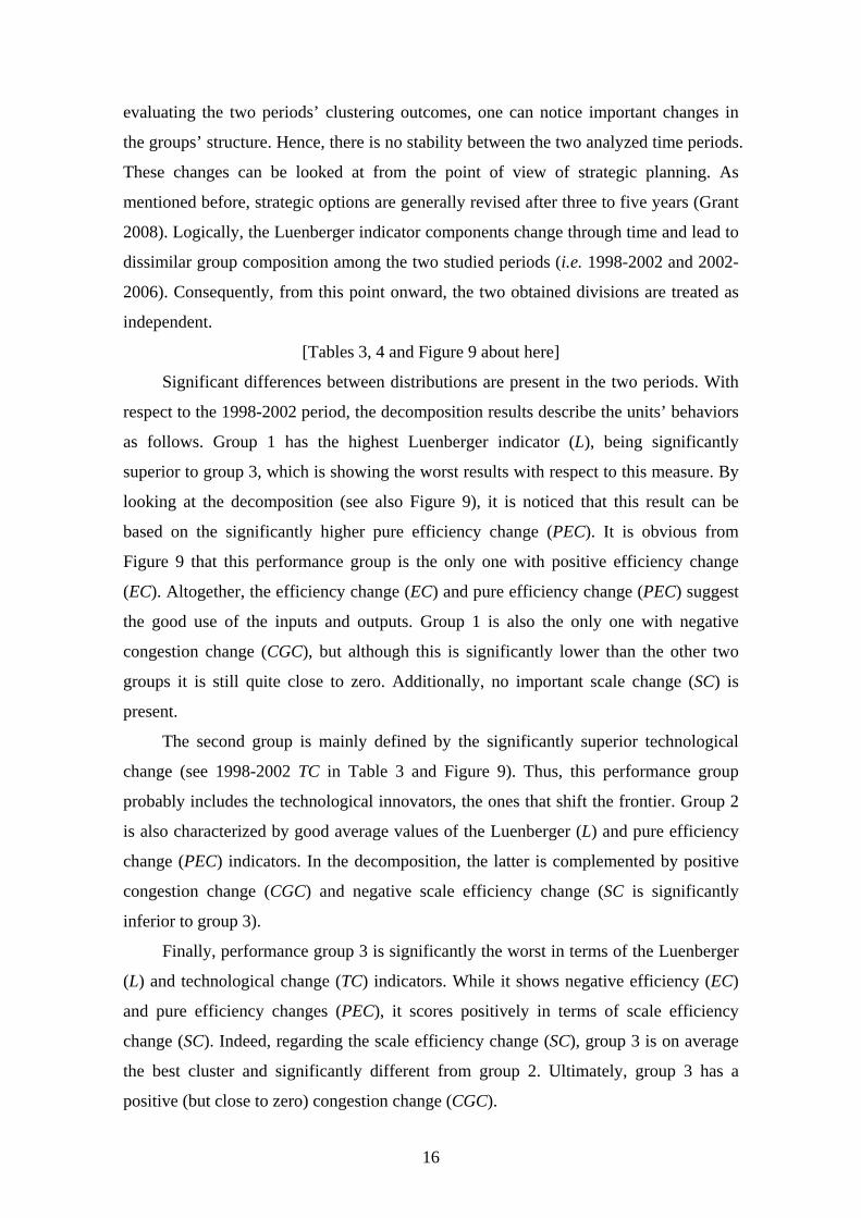
two samples. Table 1 and Figure 4 present the associated descriptive statistics. Notice

that the entire analyzed sample is maintained as no infeasibilities appear in the

computations. With respect to the studied years, the Spanish banking sector is showing

–up to a certain extent– the expected results. In terms of productivity the total

Luenberger indicator (L) scores point to general improvement since the higher value is

in the second period. This can be observed in Figure 4 through the roughly 2-to-1 ratio

between the two time periods for the mean values of the Luenberger measure (L) and

the technological change (TC). First, this could represent a continuation of the good use

of resources in the Spanish banking industry, and the increase in competition manifested

throughout the post-deregulation phase. Second, new information technologies and

innovative practices may form the basis of the positive shifts of the frontier (see the TC

results of 0.24 in 2002-2006 and 0.10 in 1998-2002).

[Figure 4 and Table 1 about here]

However, through the decomposed factors we can identify that the two periods are

not entirely similar. Even if the Luenberger indicator (L) and the technological

component (TC) are quite higher in the second period, this is not the case for the rest of

the components. At a first glance, Figure 4 illustrates the sign differences for efficiency

14

change (EC), pure efficiency change (PEC) and congestion change (CGC). The

efficiency change (EC) decreased from 0.0136 to -0.018 hinting that albeit 2002 was

better than 1998 in terms of efficiency, this rising trend did not continue to 2006. In the

utilized decomposition, this is the sum of pure efficiency change (PEC), congestion

change (CGC) and scale efficiency change (SC).

On the one hand, the positive efficiency change (EC) in 2002 with respect to 1998

may be an indication of successful management (see also the pure efficiency measure

(PEC)). On the other hand, in 2006 with 2002 as a benchmark, the pure efficiency

change (PEC) and the scale efficiency change (SC) have negative values (although not

alarming as they are in the vicinity of zero). Thus, it is possible that the territorial

expansion offered some advantages initially, while problems with the use of inputs and

outputs appeared only in the second period. Conversely, the congestion change (CGC)

results are better in the second period. This outcome is interesting in the background of

the expansion process. Nonetheless, these changes are quite close to zero, hence

congestion remains apparently non-problematic.

5.2. Relation between Private and Savings Banks According to the Luenberger Indicators

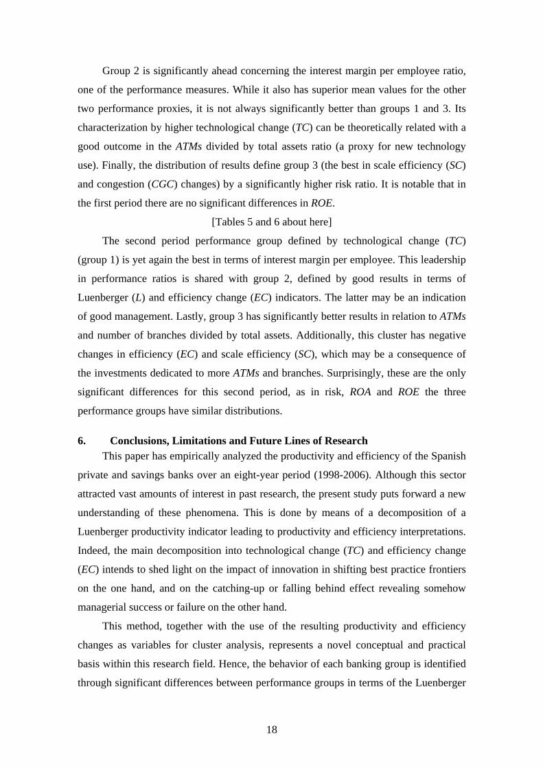
Table 2 and Figures 5 to 8 present results according to the type of bank. These are

similar to the ones related to the total sample. Moreover, as some components are

showing better results for private banks and others for savings banks, these results may

reveal there is fierce competition. Using Table 2 and Figure 5, one can note that in the

first period savings banks perform significantly better with respect to the Luenberger

indicator (L), the technological change (TC), and the pure efficiency change (PEC).

Nevertheless, we observe that private banks have better efficiency change (EC) and no

scale efficiency change (SC) problems. Thus, a speculation is that in 1998-2002 the

savings banks introduced more innovative practices and new technologies, as captured

by the technology change indicator (TC).

[Table 2 and Figures 5, 6 about here]

In the second period, the Luenberger measure (L) distributions show no significant

difference between both bank types. This is consistent with the competition assumption

in terms of productivity. Besides, the technological change (TC) mean values are

roughly equal, although there are differences in the distribution of the results.

Comparisons are shown in Table 2 and Figure 6. One can highlight the efficiency

change (EC) difference in favor of the private banks. This better efficiency change (EC)

15

of private banks is consistent with the first period, even though negative changes are

attained. In addition, all outcomes are in accordance with the interpretations in

Subsection 5.1.

[Figures 7 and 8 about here]

Further insights can be achieved comparing the private and savings banks between

the two periods on Figures 7 and 8. These figures indicate that the 2-to-1 ratio between

the two periods for the Luenberger measure (L) and the technological change (TC) (see

Subsection 5.1.) is mostly generated by the private banks. In their case this ratio is even

larger than 2-to-1, with respect to both the Luenberger (L) and technological change (TC)

indicators. At the same time, for the savings banks the same ratios are quite smaller,

showing values of 1.54 for the Luenberger indicator (L) and 1.88 in the case of

technological change (TC). Furthermore, one can also notice the inefficient employment

of inputs and outputs in the case of the savings banks. This is shown mainly by the

negative pure efficiency change (PEC) component obtained for the second analyzed

period. However, at the same time an improvement of savings banks is found in the

congestion change (CGC) indicator.

One can imagine that the labor input was congested during the expansion process

at the end of the 1990s and that, subsequently, the situation improved. Congestion

increased (see negative CGC in Table 2 and Figure 8) when the savings banks shifted

from a static market position to a growth phase involving an expansion of their number

of branches. However, once the expansion had been realized, the savings banks may

have directed their efforts to solving the congestion problem. Therefore, the congestion

change component (CGC) ends up with a positive value. For the private banks no

important movements are found in terms of the congestion (CGC) and scale efficiency

(SC) changes, both of which have values close to zero.

5.3. Performance Groups and Their Economic Interpretations

The above outcomes provide the basis for the second stage of the analysis. The

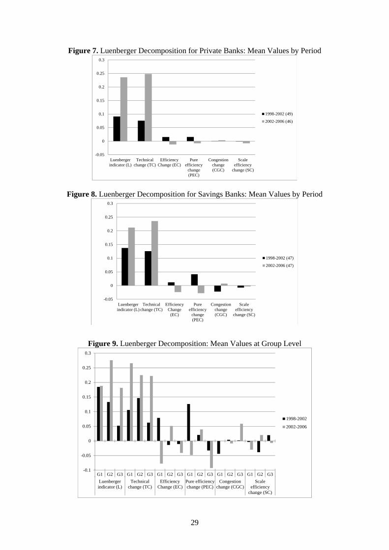
clustering results for the Luenberger decomposition are shown in Table 3 and Figure 9

(descriptive statistics) and Table 4 (Li test significance differences). For both 1998-

2002 and 2002-2006 periods, the indicated number of performance groups is three. The

discriminant analysis confirms that the groups are correctly formed, since the

predictions yield more than 90% accurate classifications. Furthermore, the clusters are

not separated as a function of bank type, but as a result of productivity scores. By

16

evaluating the two periods’ clustering outcomes, one can notice important changes in

the groups’ structure. Hence, there is no stability between the two analyzed time periods.

These changes can be looked at from the point of view of strategic planning. As

mentioned before, strategic options are generally revised after three to five years (Grant

2008). Logically, the Luenberger indicator components change through time and lead to

dissimilar group composition among the two studied periods (i.e. 1998-2002 and 2002-

2006). Consequently, from this point onward, the two obtained divisions are treated as

independent.

[Tables 3, 4 and Figure 9 about here]

Significant differences between distributions are present in the two periods. With

respect to the 1998-2002 period, the decomposition results describe the units’ behaviors

as follows. Group 1 has the highest Luenberger indicator (L), being significantly

superior to group 3, which is showing the worst results with respect to this measure. By

looking at the decomposition (see also Figure 9), it is noticed that this result can be

based on the significantly higher pure efficiency change (PEC). It is obvious from

Figure 9 that this performance group is the only one with positive efficiency change

(EC). Altogether, the efficiency change (EC) and pure efficiency change (PEC) suggest

the good use of the inputs and outputs. Group 1 is also the only one with negative

congestion change (CGC), but although this is significantly lower than the other two

groups it is still quite close to zero. Additionally, no important scale change (SC) is

present.

The second group is mainly defined by the significantly superior technological

change (see 1998-2002 TC in Table 3 and Figure 9). Thus, this performance group

probably includes the technological innovators, the ones that shift the frontier. Group 2

is also characterized by good average values of the Luenberger (L) and pure efficiency

change (PEC) indicators. In the decomposition, the latter is complemented by positive

congestion change (CGC) and negative scale efficiency change (SC is significantly

inferior to group 3).

Finally, performance group 3 is significantly the worst in terms of the Luenberger

(L) and technological change (TC) indicators. While it shows negative efficiency (EC)

and pure efficiency changes (PEC), it scores positively in terms of scale efficiency

change (SC). Indeed, regarding the scale efficiency change (SC), group 3 is on average

the best cluster and significantly different from group 2. Ultimately, group 3 has a

positive (but close to zero) congestion change (CGC).

17

Interpretations of the results are similar in the case of the period 2002-2006, even

though the composition of the performance groups and the indicator values are slightly

different. Banks in performance group 1 have by far the best results regarding

technological change (TC). Even if the mean values of this component are not that

dissimilar among the three clusters (see Table 4 and Figure 9), the Li test indicates there

are significant differences among the distributions of these scores. Consequently, one

could speculate that banks in group 1 are leading the innovations and technological

improvements. Moreover, one can also observe the downside of this technological

change (TC), as this cluster suffers from important negative changes in efficiency (EC)

and scale efficiency (SC). It may be that investments in new technologies affect the

input-output use, leading banks in this group to operate at an inefficient scale.

Group 2 is projected as the best performer through the highest Luenberger

indicator (L) and, after decomposing, experiences the highest efficiency (EC), pure

efficiency (PEC) and scale efficiency (SC) changes (see Table 4 and Figure 9).

Furthermore, concerning the last three indicators, cluster 2 is the only one with positive

values throughout. Hence, group 2 is the leader with regard to inputs and outputs

employment (see EC and PEC) and the management of scale efficiency (see SC). The

results indicate that group 3 is formed by the worst performers. Even if so, in contrast to

the negative pure efficiency change (PEC), the Luenberger (L) and technological

change (TC) indicators present quite high positive shifts. Furthermore, the congestion

change indicator (CGC) is significantly superior to the other two performance groups,

an indication of improvements in labor utilization.6

5.4. Linking Performance Groups with Banking Ratios: Supplementary Analysis

Following this characterization of performance groups, this supplementary

analysis attempts to develop some additional interpretations. By associating the banking

ratios defined in Subsection 4.2. with the performance groups, Tables 5 and 6 present

descriptive statistics and test statistics. Interpreting these results, we observe that in

1998-2002 group 1 is significantly superior regarding the proximity to customers

(number of branches divided by total assets). In addition, this performance group shares

the leading position in terms of ROA with group 2. This is in line with the fact that this

cluster is the one with the best Luenberger indicator (L) and pure efficiency change

(PEC).

6 An appendix containing graphical interpretations of the Li tests is available upon request.

18

Group 2 is significantly ahead concerning the interest margin per employee ratio,

one of the performance measures. While it also has superior mean values for the other

two performance proxies, it is not always significantly better than groups 1 and 3. Its

characterization by higher technological change (TC) can be theoretically related with a

good outcome in the ATMs divided by total assets ratio (a proxy for new technology

use). Finally, the distribution of results define group 3 (the best in scale efficiency (SC)

and congestion (CGC) changes) by a significantly higher risk ratio. It is notable that in

the first period there are no significant differences in ROE.

[Tables 5 and 6 about here]

The second period performance group defined by technological change (TC)

(group 1) is yet again the best in terms of interest margin per employee. This leadership

in performance ratios is shared with group 2, defined by good results in terms of

Luenberger (L) and efficiency change (EC) indicators. The latter may be an indication

of good management. Lastly, group 3 has significantly better results in relation to ATMs

and number of branches divided by total assets. Additionally, this cluster has negative

changes in efficiency (EC) and scale efficiency (SC), which may be a consequence of

the investments dedicated to more ATMs and branches. Surprisingly, these are the only

significant differences for this second period, as in risk, ROA and ROE the three

performance groups have similar distributions.

6. Conclusions, Limitations and Future Lines of Research

This paper has empirically analyzed the productivity and efficiency of the Spanish

private and savings banks over an eight-year period (1998-2006). Although this sector

attracted vast amounts of interest in past research, the present study puts forward a new

understanding of these phenomena. This is done by means of a decomposition of a

Luenberger productivity indicator leading to productivity and efficiency interpretations.

Indeed, the main decomposition into technological change (TC) and efficiency change

(EC) intends to shed light on the impact of innovation in shifting best practice frontiers

on the one hand, and on the catching-up or falling behind effect revealing somehow

managerial success or failure on the other hand.

This method, together with the use of the resulting productivity and efficiency

changes as variables for cluster analysis, represents a novel conceptual and practical

basis within this research field. Hence, the behavior of each banking group is identified

through significant differences between performance groups in terms of the Luenberger

19

indicator and its components. In this manner, the productivity and efficiency results and

those of the cluster analysis are consistent with each other, an issue that attracted quite a

lot of debate in the strategic groups’ literature.

The proposed methods were devised in the framework of offering a

comprehensive description of the evolution of the Spanish banking sector. Apart from

the above empirical findings, other interesting phenomena are revealed. For instance,

taking advantage of the deregulation, the savings banks initiated an important expansion

process. This movement from the static market situation to the growth phase seems to

have created congestion issues in the labor input. These have probably been solved by

investments in new technologies dedicated to the high number of branches that had to

be organized. Furthermore, according to the analyzed time periods, local scale

economies appear to have been exhausted (thus, no efficiency gains seem to remain

possible from internal growth). In this respect, future research could be directed to

branch network optimization through potential mergers and acquisitions aimed at

increasing efficiency. These operations could have a positive impact not only on the

scale efficiency, but also on the scope efficiency of the Spanish banking industry.

Obviously, each empirical work must acknowledge its methodological and sample

related limitations. First, the time-span of the sample can be enlarged. Second,

international comparisons could be introduced when certain similarities in behaviors

can be encountered. These are among the issues that could be fruitful avenues for future

work.

References:

Amel, D. F., Rhoades, S. A., 1988. Strategic Groups in Banking. Review of Economics and Statistics 70 (4), 685-689.

Andersen, P., Petersen, N.C., 1993. A Procedure for Ranking Efficient Units in Data Envelopment Analysis. Management Science 39 (10), 1261-1264.

Athanassopoulos, A.D., 2003. Strategic Groups, Frontier Benchmarking and Performance Differences: Evidence from the UK Retail Grocery Industry. Journal of Management Studies 40 (4), 921-953.

Barney, J.B., Hoskisson, R.E., 1990. Strategic Groups: Untested Assertions and Research Proposals. Managerial and Decision Economics 11 (3), 187-198.

Barros, C.P., Menezes, A.G., Vieira, J.C., Peypoch, N., Solonandrasana, B., 2008. An Analysis of Hospital Efficiency and Productivity Growth Using the Luenberger Indicator. Health Care Management Science 11 (4), 373-381.

Berger, A., Humphrey D., 1997. The Efficiency of Financial Institutions: International Survey and Directions for Future Research. European Journal of Operational Research 98 (2), 175-212.

20

Briec, W., 1997. A Graph Type Extension of Farrell Technical Efficiency Measure. Journal of Productivity Analysis 8 (1), 95-110.

Briec, W., Kerstens, K. 2009. The Luenberger Productivity Indicator: An Economic Specification Leading to Infeasibilities. Economic Modelling 26 (3), 597-600.

Bos, J.W.B, Kool, C.J.M., 2006. Bank Efficiency: The Role of Bank Strategy and Local Market Conditions. Journal of Banking and Finance 30 (7), 1953-1974.

Boussemart, J.-P., Briec, W., Kerstens, K., Poutineau, J.-C., 2003. Luenberger and Malmquist Productivity Indices: Theoretical Comparisons and Empirical Illustration. Bulletin of Economic Research 55 (4), 391-405.

Caves, R.E., Porter, M.E., 1977. From Entry Barriers to Mobility Barriers: Conjectural Decisions and Contrived Deterrence to New Competition. Quarterly Journal of Economics 91 (2), 421-441.

Chambers, R.G., Färe, R., Grosskopf, S., 1996. Productivity Growth in APEC Countries. Pacific Economic Review 1 (3), 181-190.

Chambers, R.G., 2002. Exact Nonradial Input, Output, and Productivity Measurement. Economic Theory 20 (4), 751-765.

Cool, K., Schendel, D., 1987. Strategic Group Formation and Performance: The Case of the US Pharmaceutical Industry, 1963–1982. Management Science 33 (9), 1102-124.

Crespí, R., García-Cestona, M., Salas, V., 2004. Governance Mechanisms in Spanish Banks. Does Ownership Matter? Journal of Banking and Finance 28 (10), 2311-2330.

Cuesta, R.A., Orea, L., 2002. Mergers and Technical Efficiency in Spanish Savings Banks: A Stochastic Distance Function Approach. Journal of Banking and Finance 26 (12), 2231-2247.

Day, D.L., Lewin, A.Y., Li, H., Salazar, R., 1994. Strategic Leaders or Strategic Groups: A Longitudinal Analysis of Outliers. In: Charnes, A., Cooper, W.W., Lewin, A.Y., Seiford, L.M. (Eds.), Data Envelopment Analysis Theory, Methodology and Applications. Kluwer, Boston.

Day, D.L., Lewin, A.Y., Li, H., 1995. Strategic Leaders or Strategic Groups: A Longitudinal Data Envelopment Analysis of the US Brewing Industry. European Journal of Operational Research 80 (3), 619-638.

Diewert, W.E., 2005. Index Number Theory Using Differences Rather Than Ratios. The American Journal of Economics and Sociology 64 (1), 311-360.

Färe, R., Grosskopf, S., Lindgren, B., Roos, P., 1992. Productivity Changes in Swedish Pharmacies 1980-1989: A Nonparametric Malmquist Approach. Journal of Productivity Analysis 3 (1-2), 85-101.

Färe, R., Grosskopf, S., Lovell, C.A.K., 1994. Production Frontiers. Cambridge University Press, New York.

Färe, R., Grosskopf, S., Roos, P., 1998. Malmquist Productivity Indices: A Survey of Theory and Practice. in: R. Färe, S. Grosskopf, R. Russell (eds) Index Numbers: Essays in Honour of Sten Malmquist, Kluwer, Boston.

Färe, R., Grosskopf, S., 2000. Decomposing Technical Efficiency with Care. Management Science 46 (1), 167-168.

Fethi, M.D., Pasiouras F., 2010. Assessing Bank Efficiency and Performance with Operational Research and Artificial Intelligence Techniques: A Survey. European Journal of Operational Research 204 (2), 189-198.

Fiegenbaum, A., Thomas, H., 1994. The Concept of Strategic Groups as Reference Groups: An Adaptive Model and an Empirical Test. In Daems, H., Thomas, H. (Eds), Strategy Groups, Strategic Moves and Performance. Oxford: Pergamon.

21

Goddard, J.A., Molyneux, P., Wilson, J.O.S., 2001. European Banking: Efficiency, Technology and Growth. Wiley, New York.

Grant, R.M., 2008. Contemporary Strategy Analysis (6th ed.). Blackwell, Malden. Grifell-Tatjé, E., Lovell, C.A.K., 1996. Deregulation and Productivity Decline: The case

of Spanish Saving Banks. European Economic Review 40 (6), 1281-1303. Grifell-Tatjé, E., Lovell, C.A.K. 1997. The Sources of Productivity Change in Spanish

Banking. European Journal of Operational Research 98 (2), 364-380. Hatten, K.J., Hatten, M.L., 1987. Strategic Groups, Asymmetrical Mobility Barriers and

Contestability. Strategic Management Journal 8 (4), 329-342. Hunt, M.S., 1972. Competition in the Major House Appliance Industry 1960–1970.

Ph.D. dissertation, Harvard University. Ketchen, D.J., Shook, C., 1996. The Application of Cluster Analysis in Strategic

Management Research: An Analysis and Critique. Strategic Management Journal 17 (6), 441-458.

Kolari, J., Zardkoohi A., 1987. Bank Costs, Structure, and Performance. D.C. Heath, Lexington.

Kumar, S., Russell, R., 2002. Technological Change, Technological Catch-up, and Capital Deepening: Relative Contributions to Growth and Convergence. American Economic Review 92 (3), 527-548.

Li, Q., 1996. Nonparametric Testing of Closeness between Two Unknown Distribution Functions. Econometric Reviews 15 (3), 261-274.

Lozano-Vivas, A., 1997. Profit Efficiency for Spanish Savings Banks. European Journal of Operational Research 98 (2), 381-394.

Luenberger, D.G., 1992. New Optimality Principles for Economic Efficiency and Equilibrium. Journal of Optimization Theory and Applications 75 (2), 221-264.

Managi, S., 2003. Luenberger and Malmquist Productivity Indices in Japan, 1955-1995. Applied Economics Letters 10 (9), 581-584.

Más-Ruíz F.J., Nicolau-Gonzalbez J.L., Ruiz-Moreno F., 2005. Asymmetric Rivalry between Strategic Groups: Response, Speed and Response and Ex-Ante versus Ex-Post Competitive Interaction in the Spanish Bank Deposit Market. Strategic Management Journal 26 (8), 713-745.

Mehra, A., 1996. Resource and Market Based Determinants of Performance in the US Banking Industry. Strategic Management Journal 17 (4), 307-322.

Mussard, S., Peypoch, N., 2006. On Multi-Decomposition of the Aggregate Luenberger Productivity Index. Applied Economics Letters 13 (2), 113-116.

Po, R.-W., Guh, Y.-Y., Yang, M.-S., 2009. A New Clustering Approach Using Data Envelopment Analysis. European Journal of Operational Research 199 (1), 276-284.

Porter, M.E., 1979. The Structure within Industries and Companies Performance. Review of Economics and Statistics 61 (2), 224-227.

Porter, M.E., 1980. Competitive Strategy: Techniques for Analysing Industries and Competitors. Free Press, New York.

Prior, D., 2003. Long- and Short-run Non-parametric Cost Frontier Efficiency: An Application to Spanish Savings Banks. Journal of Banking and Finance 27 (4), 655-671.

Prior, D., Surroca, J., 2006. Strategic Groups Based on Marginal Rates: An Application to the Spanish Banking Industry. European Journal of Operational Research 170 (1), 293-314.

Ray, S.C.., Das, A., 2010. Distribution of Cost and Profit Efficiency: Evidence from Indian Banking. European Journal of Operational Research 201 (1), 297-307.

22

Short, J.C., Ketchen, D.J., Palmer, T.B., Hult, T. M., 2007. Firm, Strategic Group, and Industry Influences on Performance. Strategic Management Journal 28 (2), 147-167.

Simar, L., Zelenyuk, V., 2006. On Testing Equality of Distributions of Technical Efficiency Scores. Econometric Reviews 25 (4), 497-522.

Sohn, S.Y., 2006. Random Effects Logistic Regression Model for Ranking Efficiency in Data Envelopment Analysis. Journal of the Operational Research Society 57 (11), 1289-1299.

Thomas, H., Venkatraman, N., 1988. Research on Strategic Groups: Progress and Prognosis. Journal of Management Studies 25 (6), 537-555.

Tortosa-Ausina, E., 2003. Nontraditional Activities and Bank Efficiency Revisited: A Distributional Analysis for Spanish Financial Institutions. Journal of Economics and Business 55 (4), 371-395.

Tortosa-Ausina, E., Grifell-Tatjé, E., Armero, C., Conesa, D., 2008. Sensitivity Analysis of Efficiency and Malmquist Productivity Indices: An Application to Spanish Savings Banks. European Journal of Operational Research 184 (3), 1062-1084.

Williams, J., Peypoch, N., Barros, C.P., 2009. The Luenberger Indicator and Productivity Growth: A Note on the European Savings Banks Sector. Applied Economics, First published on: 18 June 2009 (iFirst).

Wilson, P.W., 1993. Detecting Outliers in Deterministic Nonparametric Frontier Models with Multiple Outputs. Journal of Business & Economic Statistics 11 (3), 319-323.

Zúñiga-Vicente, J.A., Fuente Sabaté, J.M., Rodríguez Puerta, J., 2004. A Study of Industry Evolution in the Face of Major Environmental Disturbances: Group and Firm Strategic Behavior of Spanish Banks, 1983–1997. British Journal of Management 15 (3), 219-245.

23

Table 1. Descriptive Statistics 1998 – 2002 Mean Std. dev. Min. Max.

Total (96 units)

L 0.1138 0.1339 -0.3480 0.7031 TC 0.1002 0.0624 -0.1395 0.2913 EC 0.0136 0.1131 -0.3503 0.5090 PEC 0.0282 0.0988 -0.2546 0.5026 CGC -0.0103 0.0359 -0.1440 0.1204

SC -0.0042 0.0582 -0.2954 0.1945 2002 – 2006 Mean Std. dev. Min. Max.

Total (93 units)

L 0.2239 0.1435 -0.1632 0.8826 TC 0.2419 0.0379 0.1492 0.4176

EC -0.0180 0.1401 -0.3581 0.6859 PEC -0.0179 0.1141 -0.4333 0.5300 CGC 0.0053 0.0273 -0.0761 0.1212

SC -0.0054 0.1123 -0.5429 0.7655

Table 2. Luenberger Decomposition: Results per Bank-Type

1998 – 2002 Mean Std. Dev. Min. Max. Li Test

(t-stat./p-value) L PB (49) 0.0913 0.1787 -0.3480 0.7031 3.5280 SB (47) 0.1373 0.0510 0.0266 0.2561 0.0002* TC PB (49) 0.0758 0.0763 -0.1395 0.2913 11.5185 SB (47) 0.1256 0.0260 0.0066 0.1634 0.0000* EC PB (49) 0.0155 0.1490 -0.3503 0.5090 1.7182 SB (47) 0.0117 0.0570 -0.0987 0.2494 0.0428* PEC PB (49) 0.0157 0.1293 -0.2546 0.5026 3.1393 SB (47) 0.0412 0.0489 -0.0759 0.1478 0.0008* CGC PB (49) 0.0008 0.0320 -0.1440 0.1204 0.0754 SB (47) -0.0220 0.0363 -0.1329 0.0034 0.4699 SC PB (49) -0.0011 0.0714 -0.2954 0.1534 3.0761 SB (47) -0.0074 0.0407 -0.0957 0.1945 0.0010*

2002 – 2006 Mean Std. Dev. Min. Max. Li Test

(t-stat./p-value) L PB (46) 0.2360 0.1938 -0.1632 0.8826 1.1228 SB (47) 0.2120 0.0645 0.0401 0.3234 0.1307 TC PB (46) 0.2481 0.0478 0.1492 0.4176 1.7875 SB (47) 0.2358 0.0237 0.1725 0.2986 0.0369* EC PB (46) -0.0121 0.1900 -0.3581 0.6859 1.3167 SB (47) -0.0238 0.0624 -0.2040 0.0762 0.0939* PEC PB (46) -0.0078 0.1446 -0.4333 0.5300 3.0927 SB (47) -0.0279 0.0734 -0.2524 0.1686 0.0009* CGC PB (46) 0.0034 0.0227 -0.0406 0.1212 1.3968 SB (47) 0.0073 0.0312 -0.0761 0.0843 0.0812* SC PB (46) -0.0077 0.1558 -0.5429 0.7655 0.0031 SB (47) -0.0032 0.0382 -0.1277 0.0709 0.4987

The values between parentheses represent the number of units for each of the two bank types. *: Statistically significant differences

24

Table 3. Luenberger Decomposition: Group Level Descriptive Statistics 1998-2002 Mean Std. Dev Min. Max.

L G1 (27) 0.1849 0.1443 -0.0625 0.7032 G2 (29) 0.1331 0.1003 -0.1753 0.4173 G3 (40) 0.0520 0.1219 -0.3481 0.2562 TC G1 (27) 0.1060 0.0604 -0.1396 0.1941 G2 (29) 0.1467 0.0409 0.0903 0.2913 G3 (40) 0.0625 0.0528 -0.0837 0.1521 EC G1 (27) 0.0789 0.1346 -0.1412 0.5091 G2 (29) -0.0136 0.0811 -0.2954 0.1259 G3 (40) -0.0106 0.1016 -0.3504 0.2495 PEC G1 (27) 0.1263 0.1032 0.0000 0.5027 G2 (29) 0.0207 0.0338 -0.0564 0.0943 G3 (40) -0.0324 0.0736 -0.2547 0.0562 CGC G1 (27) -0.0440 0.0458 -0.1441 0.0235 G2 (29) 0.0040 0.0224 -0.0053 0.1204 G3 (40) 0.0019 0.0171 -0.0254 0.0616 SC G1 (27) -0.0034 0.0362 -0.0868 0.1295 G2 (29) -0.0383 0.0624 -0.2954 0.0102 G3 (40) 0.0199 0.0560 -0.0957 0.1945

2002-2006 Mean Std. Dev Min. Max. L G1 (40) 0.1881 0.1267 -0.1632 0.4177 G2 (39) 0.2760 0.1625 0.1001 0.8827 G3 (14) 0.1813 0.0806 0.0384 0.2839 TC G1 (40) 0.2656 0.0426 0.1492 0.4177 G2 (39) 0.2248 0.0230 0.1661 0.2855 G3 (14) 0.2221 0.0137 0.2078 0.2429 EC G1 (40) -0.0775 0.1048 -0.3581 0.1205 G2 (39) 0.0512 0.1588 -0.0871 0.6859 G3 (14) -0.0408 0.0813 -0.1746 0.0710 PEC G1 (40) -0.0479 0.1015 -0.4334 0.2305 G2 (39) 0.0395 0.1109 -0.0797 0.5300 G3 (14) -0.0926 0.0825 -0.2496 0.0000 CGC G1 (40) 0.0003 0.0033 -0.0079 0.0162 G2 (39) -0.0085 0.0172 -0.0761 0.0118 G3 (14) 0.0586 0.0260 0.0198 0.1212 SC G1 (40) -0.0299 0.1114 -0.5430 0.1510 G2 (39) 0.0202 0.1268 -0.1278 0.7656 G3 (14) -0.0068 0.0342 -0.0784 0.0672

The values between parentheses represent the number of units in each performance group.

25

Table 4. Luenberger Decomposition: Group Level Li Test Results

1998-2002 L TC EC PEC CGC SC 1-2 t-statistic -0.9252 2.9869 -0.1241 8.4102 8.4075 -0.2935

p-value 0.8226 0.0014* 0.5494 0.0000* 0.0000* 0.6154 1-3 t-statistic 1.6250 2.3543 -0.2561 15.0102 7.2367 0.5506

p-value 0.0520* 0.0093* 0.6011 0.0000* 0.0000* 0.2909 2-3 t-statistic 1.4446 10.4305 -0.4754 1.2284 0.2787 1.8317

p-value 0.0742* 0.0000* 0.6827 0.1097 0.3902 0.0335* 2002-2006 L TC EC PEC CGC SC

1-2 t-statistic 2.4803 8.2849 3.5531 0.8777 1.5093 1.2334 p-value 0.0065* 0.0000* 0.0002* 0.1901 0.0656* 0.1087

1-3 t-statistic 0.3478 5.9275 -0.4415 0.3129 19.6905 -0.1518 p-value 0.3640 0.0000* 0.6706 0.3772 0.0000* 0.5603

2-3 t-statistic -0.3185 1.4633 0.0702 1.8262 12.4554 -0.6496 p-value 0.6250 0.0716* 0.4720 0.0339* 0.0000* 0.7420

*: Statistically significant differences

Table 6. Banking Ratios: Group Level Li Test Results

1998-2002 ATM/TA Branch/TA IntMarg/Empl Risk ROA ROE 1-2 t-statistic 1.1862 2.0643 1.7500 1.9076 -0.0899 0.2440

p-value 0.1178 0.0194* 0.0401* 0.0282* 0.5358 0.4036 1-3 t-statistic 2.8309 1.9593 1.2515 1.5452 1.4487 0.7457

p-value 0.0023* 0.0250* 0.1054 0.0611* 0.0737* 0.2279 2-3 t-statistic 3.5312 1.4237 2.9858 1.8801 2.8987 0.6675

p-value 0.0002* 0.0773* 0.0014* 0.0300* 0.0019* 0.2522 2002-2006 ATM/TA Branch/TA IntMarg/Empl Risk ROA ROE

1-2 t-statistic 0.8057 1.5894 -0.3467 -0.7213 -0.3679 -0.5221 p-value 0.2102 0.0559* 0.6356 0.7646 0.6435 0.6992

1-3 t-statistic 3.0411 5.3988 2.3343 -0.1715 0.0712 -0.0161 p-value 0.0012* 0.0000* 0.0098* 0.5681 0.4716 0.5064

2-3 t-statistic 1.1569 1.0685 2.7114 0.4788 0.5022 0.0009 p-value 0.0836* 0.0926* 0.0034* 0.3160 0.3078 0.4996

*: Statistically significant differences

26

Table 5. Banking Ratios: Group Level Descriptive Statistics

1998-2002 Mean Std. Dev Min. Max. ATM/TA G1 (27) 0.000064 0.000035 0.000000 0.000145 G2 (29) 0.000049 0.000026 0.000000 0.000091 G3 (40) 0.000036 0.000035 0.000000 0.000120 Branch/TA G1 (27) 0.000063 0.000030 0.000001 0.000133 G2 (29) 0.000046 0.000019 0.000013 0.000082 G3 (40) 0.000048 0.000039 0.000000 0.000208 IntMarg/Empl G1 (27) 89.8485 18.9074 54.2858 126.1127 G2 (29) 117.7374 35.7944 71.3838 257.5769 G3 (40) 78.8165 34.8450 6.0652 140.5075 Risk G1 (27) 0.0908 0.0394 0.0526 0.2069 G2 (29) 0.0910 0.0492 0.0509 0.3330 G3 (40) 0.1077 0.0843 0.0270 0.4616 ROA G1 (27) 0.0093 0.0100 -0.0143 0.0407 G2 (29) 0.0112 0.0083 -0.0195 0.0367 G3 (40) 0.0099 0.0110 -0.0304 0.0348 ROE G1 (40) 0.0792 0.0661 -0.1017 0.2410 G2 (39) 0.1001 0.0601 -0.1785 0.1756 G3 (14) 0.0807 0.0790 -0.2256 0.2765

2002-2006 Mean Std. Dev Min. Max. ATM/TA G1 (40) 0.000030 0.000025 0.000000 0.000110 G2 (39) 0.000037 0.000027 0.000000 0.000091 G3 (14) 0.000056 0.000019 0.000026 0.000096 Branch/TA G1 (40) 0.000027 0.000017 0.000000 0.000071 G2 (39) 0.000037 0.000023 0.000000 0.000126 G3 (14) 0.000057 0.000027 0.000036 0.000144

IntMarg/Empl G1 (40) 121.5403 84.2901 6.2577 513.1580 G2 (39) 113.4744 44.8215 11.9998 187.5181 G3 (14) 95.4188 18.1373 64.4998 134.9569 Risk G1 (40) 0.1211 0.2062 0.0301 1.3488 G2 (39) 0.1147 0.1023 0.0261 0.5246 G3 (14) 0.0746 0.0129 0.0566 0.0954 ROA G1 (40) 0.0085 0.0061 -0.0072 0.0287 G2 (39) 0.0052 0.0233 -0.1271 0.0279 G3 (14) 0.0081 0.0028 0.0009 0.0127 ROE G1 (40) 0.0842 0.0480 -0.0773 0.1583 G2 (39) 0.0820 0.0763 -0.2429 0.2378 G3 (14) 0.0853 0.0282 0.0060 0.1154

The values between parentheses represent the number of units for each of the two bank types.

27

Figure 1. Efficiency Change and Technological Change y

x0

ykt

ykt+1

Tt(xt,yt|CRS, SD)

Tt+1(xt+1,yt+1|CRS, SD)

xkt xk

t+1-xt

(xkt,yk

t)

(xkt+1,yk

t+1)

Dt+1(xt+1,yt+1|CRS,SD)

-xt+1

Dt(xt,yt|CRS,SD)

Figure 2. Scale Inefficiency (adapted from Färe et al. 1994: 75) y

x0

(xlt,yl

t)

(xkt,yk

t)

Tt(xt,yt|CRS, SD)Tt(xt,yt|VRS, SD)

ylt

ykt

xltxk

t-xkt-xl

t

Figure 3. Input Congestion (Färe et al. 1994: 76)

Lt(yt|VRS,WD)

Lt(yt|VRS,SD)

x2t

x1t0

xjt

xkt

28

Figure 4. Luenberger Decomposition: Sample Mean Values

-0.05

0

0.05

0.1

0.15

0.2

0.25

0.3

Luenbergerindicator (L)

Technicalchange (TC)

EfficiencyChange (EC)

Pureefficiency

change (PEC)

Congestionchange(CGC)

Scaleefficiency

change (SC)

1998-2002 (96)

2002-2006 (93)

Figure 5. Luenberger Decomposition for 1998-2002: Mean Values by Bank Type

-0.05

0

0.05

0.1

0.15

0.2

0.25

0.3

Luenbergerindicator

(L)

Technicalchange(TC)

EfficiencyChange

(EC)

Pureefficiency

change(PEC)


Scaleefficiency

change(SC)

Private Banks (49)

Savings Banks (47)

Figure 6. Luenberger Decomposition for 2002-2006: Mean Values by Bank Type

-0.05

0

0.05

0.1

0.15

0.2

0.25

0.3




Pureefficiency

change(PEC)


Scaleefficiency

change (SC)

Private Banks (46)

Savings Banks (47)

29

Figure 7. Luenberger Decomposition for Private Banks: Mean Values by Period

-0.05

0

0.05

0.1

0.15

0.2

0.25

0.3




Pureefficiency

change(PEC)


Scaleefficiency

change (SC)

1998-2002 (49)

2002-2006 (46)

Figure 8. Luenberger Decomposition for Savings Banks: Mean Values by Period

-0.05

0

0.05

0.1

0.15

0.2

0.25

0.3



EfficiencyChange

(EC)

Pureefficiency

change(PEC)


Scaleefficiency

change (SC)

1998-2002 (47)

2002-2006 (47)

Figure 9. Luenberger Decomposition: Mean Values at Group Level

-0.1

-0.05

0

0.05

0.1

0.15

0.2

0.25

0.3

G1 G2 G3 G1 G2 G3 G1 G2 G3 G1 G2 G3 G1 G2 G3 G1 G2 G3




Pure efficiencychange (PEC)

Congestionchange (CGC)

Scaleefficiency

change (SC)

1998-2002

2002-2006

Documents

Bank Productivity and Performance Groups: A Decomposition