Embed Size (px)
Citation preview

C CO CO C CO COD
C CO C CO CO CO C CO COD
C CO C CO CO CO C CO COD
C CO C CO CO CO C CO COD
C CO C CO CO CO C CO COD
C CO C CO CO CO C CO COD
C CO C CO CO CO C CO COD
C CO C CO CO CO C CO COD
C CO C CO CO CO C CO COD
C CO C CO CO CO C CO COD
C CO C CO CO CO C CO COD
C CO C CO CO CO C CO COD
C CO C CO CO CO C CO COD
C CO C CO CO CO C CO COD
C CO C CO CO CO C CO COD
C CO C CO CO CO C CO COD
C CO C CO CO CO C CO COD
C CO C CO CO CO C CO COD
C CO C CO CO CO C CO COD
C CO C CO CO CO C CO COD
C CO C CO CO CO C CO COD
C CO C CO CO CO C CO COD
C CO C CO CO CO C CO COD
C CO C CO CO CO C CO COD
C CO C CO CO CO C CO COD
C CO C CO CO CO C CO COD
C CO C CO CO CO C CO COD
C CO C CO CO CO C CO COD
C CO C CO CO CO C CO COD
C CO C CO CO CO C CO COD
Staff Working Paper No. 549How much do investors pay for houses? Philippe Bracke
September 2015
Staff Working Papers describe research in progress by the author(s) and are published to elicit comments and to further debate. Any views expressed are solely those of the author(s) and so cannot be taken to represent those of the Bank of England or to stateBank of England policy. This paper should therefore not be reported as representing the views of the Bank of England or members ofthe Monetary Policy Committee, Financial Policy Committee or Prudential Regulation Authority Board.

Staff Working Paper No. 549How much do investors pay for houses?Philippe Bracke(1)
Abstract
In 2013 buy-to-rent investors — referred to as buy-to-let (BTL) in the United Kingdom — accountedfor 13% of all UK mortgage-funded housing transactions and for an even greater fraction of non-mortgage sales. This paper studies the behaviour of BTL investors using 2009–14 micro data.Combining the universe of transactions from the England and Wales Land Registry with online listingsfrom WhenFresh/Zoopla, I identify a BTL purchase as a transaction where a rental listing on the sameproperty appears on the web in the six subsequent months. The micro data reproduce the increase inBTL transactions over 2009–14 and show that BTL investors are more likely to invest in regions withlarge rental markets. I find that, on average, BTL investors pay 0.9%–1.1% less than other buyers forequivalent properties. Discounts are larger (around 2%) in regions with less liquid housing markets.Results are robust to including detailed geographical fixed effect and advertised sale prices in theregressions. I also show that properties purchased by investors spend on average five days less on themarket.
Key words: House prices, rents, real estate investors.
JEL classification: R21, R31.
(1) Bank of England and Spatial Economics Research Centre (LSE). Email: [email protected].
The views expressed in this paper are those of the author, and not necessarily those of the Bank of England or its committees. I thank seminar participants at Reading Business School, IMF, Bank of England, LSE, and the 2015 Royal Economic SocietyConference, as well as Hites Ahir, Eduard Andreu, Paul Cheshire, Christian Hilber, Francis Salway, and several Bank ofEngland colleagues for useful comments and suggestions. I am grateful to Perttu Korhonen for his work on matching housingdata sets and to Mark Cunningham and Alan Dean of WhenFresh.com for helping me with the Zoopla listings.
Information on the Bank’s working paper series can be found atwww.bankofengland.co.uk/research/Pages/workingpapers/default.aspx
Publications Team, Bank of England, Threadneedle Street, London, EC2R 8AH Telephone +44 (0)20 7601 4030 Fax +44 (0)20 7601 3298 email [email protected]
© Bank of England 2015ISSN 1749-9135 (on-line)

Staff Working Paper No. 549 September 2015 1
1 Introduction
Buy‐to‐rent investors – known as buy‐to‐let (BTL) in the UK – are taking on an increasingly important
role in housing markets. In terms of flow, according to the Council of Mortgage Lenders (CML), BTL
accounted for 13% of UK mortgage lending in 2013.1 BTL activity is also associated to a significant
share of non‐mortgage house purchases, for which official estimates are not available (some
estimates are provided in the present paper). In terms of stock, data from the Department of
Communities and Local Government show that the UK stock of housing held for private renting has
more than doubled in the past 15 years, from 9% of the total stock in 2000 to 19% of the stock in
2013.2 These trends are common to the US, where home ownership is also declining (Jones and
Richardson, 2014).
An important policy issue is whether BTL investors push up prices and contribute to macro‐financial
instability or, to the contrary, play a helpful role as buyers of last resort and contribute to market
clearing (Molloy and Zarutskie, 2013). The Bank of England Financial Policy Committee (FPC) has
recently expressed the concern that `[t]he scale and nature of BTL activity makes it a significant
potential amplifier of housing and credit cycles’.3 The UK Government intends to consult on tools
related to BTL lending later in 2015, with the objective of building an in‐depth evidence base on how
activity in the UK BTL housing market may carry risks to financial stability.4
The effect of BTL activity on house prices can be direct, when BTL investors systematically bid more
than other buyers for the same houses, or indirect, when the arrival of a new group of buyers pushes
market prices up (without necessarily implying that the new buyers pay more on average). In this
paper I focus on the direct effect of the flow of investor purchases and consider both mortgage‐ and
non‐mortgage‐funded BTL.5 A systematic pattern of investors overpaying for properties could
endanger macro‐financial stability by exacerbating house price rises, potentially leading to
overextension of credit. Also, it is often suggested in the media that investors drive other purchasers
(such as First Time Buyers, FTB) out of the market.6
Economic theory does not provide an unambiguous prediction on the direct effect of BTL on house
prices. On the one hand, homeowners may bid higher than investors because of idiosyncratic tastes
1 https://www.cml.org.uk/cml/publications/newsandviews/150/585. 2 Another 18% of the stock is classified as social renting (i.e. renting from a local authority or housing association) and the remaining is owner‐occupied housing. 3 Financial Policy Committee statement from its policy meeting, 26 September 2014, available at http://www.bankofengland.co.uk/publications/Pages/news/2014/080.aspx. 4 According to the 2012 Financial Services Act the FPC can direct the Prudential Regulation Authority (PRA) and the Financial Conduct Authority (FCA) to implement specific macro‐prudential measures to improve the resilience of the UK financial system. To address its concerns on mortgage‐funded BTL activity, the FPC has asked the UK Government for powers of Direction on BTL. 5 Most non‐mortgage transactions are likely to be financed by cash. However, this group can also contain transactions by large private investors with access to other financing methods (such as banks’ corporate credit books or capital markets). 6 See for instance `Wild West buy‐to‐let investors force first‐time buyers off the housing ladder', Telegraph, 11 July 2011
Staff Working Paper No. 549 September 2015 2
for specific property features (as in search‐and‐matching models of the housing market7), or because
ownership acts as an insurance against rent risk (Sinai and Souleles, 2005). On the other hand,
investors may be more efficient than homeowners at managing and renovating properties
(Linneman, 1985). To further complicate the issue, homeowners and landlords are subject to
different tax regimes (Chambers et al, 2009a) and access different types of mortgages (Chambers et
al, 2009b). In the absence of a clear theoretical prediction, the question of whether BTL investors
pay more for houses must be answered by the data.
The empirical strategy of this paper is based on the increasing importance of internet portals in
advertising rental properties. The key idea is that, if a flat or house is advertised for rent shortly after
its purchase, it is a BTL property.8 I use two data sources to implement this approach: the Land
Registry, which contains all residential transactions in England and Wales, and WhenFresh.com, a
company that processes the listings of Zoopla, the second most popular UK property portal in terms
of traffic. This method allows me to detect, at the end of the sample (2014Q1), between one quarter
and one fifth of all mortgage‐funded BTL purchases in the UK, and approximately the same
proportion of non‐mortgage BTL transactions.9
Because this paper is the first to study UK housing investors using micro data, I show some
descriptive statistics on BTL activity before turning to the main research question. Zoopla started its
activity in November 2008, therefore the sample includes the quarters from 2009Q1 to 2014Q1. The
micro data show that BTL transactions have doubled in this period, consistent with aggregate data
from other sources such as the CML.10 From a cross‐sectional perspective, BTL transactions are
concentrated in places with a large private rented housing stock (such as dense urban areas) and in
types of properties which have traditionally been associated with renting (i.e. flats rather than
houses). The probability that a BTL investment is resold within the first 6 years is lower than for the
rest of the housing stock – this confirms that the paper focuses on long‐term investors rather than
on short‐term buy‐to‐sell.
To answer the main research question, I run a regression of individual sale prices on a BTL indicator,
controlling for available property characteristics and local market conditions (through postcode‐
month fixed effects). The possibility of unmeasured property attributes affecting the results is the
main econometric challenge. To address it, I restrict attention to those properties for which a sale
listing exists in Zoopla and include the advertised price in the regression.11 Together with the other
7 The literature on search‐and‐matching in the housing market includes, for instance, Wheaton (1990), Albrecht et al (2007), and Ngai and Tenreyro (2014). However these papers do not distinguish between matches for owner‐occupation, investment, and rental. Halket and Pignatti (2014) discuss the household tenure decision and draw a connection between expected duration in the property and match quality. 8 In the paper, I identify BTL purchases as transactions where a rental advertisement follows a sale on the same property during the following 6 months. I also experimented with different thresholds (3 or 12 months), which yielded very similar results. 9 As shown in the Data section, the CML reports that there were 24,000 BTL mortgages for house purchase issued in 2014Q1, and I am able to identify around 5,000 of them in my sample. I also show that the number of mortgage BTL transactions is approximately the same as the number of non‐mortgage BTL transactions. 10 The total number of housing transactions went up by 85% in the same period, implying an increasing share of BTL purchases. 11 A few recent papers that use listing prices in their empirical analysis, for example to measure the effect of foreclosures on nearby property prices (Anenberg and Kung, 2014) or the effect of credit availability on house prices (Kung, 2015).

Staff Working Paper No. 549 September 2015 3
controls, the advertised price captures all information related to the value of the property known by
the seller. The baseline estimate shows a statistically significant 1.0% discount associated with BTL
transactions, implying that BTL investors spend on average less than other buyers (or, equivalently,
other buyers spend more than BTL investors). Because I do not identify all BTL transactions, I am
effectively comparing BTL sales with a control group that includes both non‐BTL and BTL properties,
and the 1.0% estimate can be considered a lower bound of the true BTL discount.
English regions and Wales have experienced diverse housing market conditions over 2009‐2014.
London has seen robust house price growth, especially in the last part of the sample;12 the South
West and South East of England have also performed well; the remaining regions have been lagging,
with some parts of the country persistently experiencing negative nominal house price growth.
Policy makers may be interested in how the BTL discount evolves in these different housing market
conditions. This analysis may also shed light on the economic mechanisms behind the discounts. In a
second set of results, I show that discounts are larger in regions with smaller private rented markets
and in the earlier years of the sample. For instance, in 2010 houses sold to BTL investors outside
London and the South of England achieved an average discount close to 2%.
Persistent BTL discounts for equivalent properties can exist in a market with search frictions. A seller
that decides to reject an investor’s bid can end up waiting a long time before a new offer arrives.
According to this view, BTL discounts are a compensation for market clearing and should be larger
when market liquidity is lower. To test this hypothesis, I measure Time‐On‐Market (TOM), the time it
takes a property to go from a Zoopla sale listing to a registered sale. I find that properties sold to
investors spend five days less on the market than other properties and TOM reductions by region
and year track average BTL discounts. Interestingly, in the last part of the sample BTL price and TOM
discounts are hardly distinguishable from zero (especially in London), suggesting that the market‐
clearing contribution of BTL investors becomes less valuable once the housing market has resumed a
sustained level of activity.
From a policy perspective, it is important to distinguish between mortgage and non‐mortgage
transactions, not least because the literature has highlighted the potential adverse effect of
increased credit availability on investors’ behaviour (Haughwout et al, 2014). Anecdotal evidence
suggests that non‐mortgage transactions are quicker because buyers do not need to obtain banks’
approval. The analysis confirms that non‐mortgage transactions are associated with a lower TOM.
This enhanced speed may allow non‐mortgage buyers to obtain higher discount, although the data
does not support this conclusion: there is no statistical difference in the price paid by mortgage and
non‐mortgage buyers.13 To the best of my knowledge, no other study in the literature has compared
the price paid in mortgage and non‐mortgage housing transactions before.
12 London house prices rose by 20% between August 2013 and August 2014 according to the Land Registry (http://landregistry.data.gov.uk/app/hpi/). 13 A similar hypothesis relates BTL discounts to the absence of a `chain’, i.e. BTL investors do not need to sell their current property before buying a new one (as in Rosenthal, 1997, or Anenberg and Bayer, 2013). In the Appendix of the paper, I compare the discounts obtained by BTL investors with those obtained by first‐time buyers, who are also unencumbered by the need to sell a property before their next purchase. I find that first‐time buyers do not enjoy a statistical significant discount, making it difficult to attribute the BTL discount to the absence of a chain.

Staff Working Paper No. 549 September 2015 4
The contribution of this paper is twofold. First, the paper shows how to identify housing investors
when the names of buyers and sellers are not available. This methodology is used here to estimate
the price paid by BTL investors, but can have other applications – for instance, it can be used by
mortgage providers to check whether owner‐occupier mortgages are being used to finance a BTL
investment. Second, this study contributes to the academic and policy debate on the role of
investors in the housing market (see the next section for a brief review of the literature). By showing
that BTL properties are sold at a discount in non‐boom periods, this paper provides evidence on the
market‐clearing contribution of housing investors. At the same time the paper shows that BTL
discounts tend to vanish when housing liquidity improves.
The rest of the paper proceeds as follows. The next section examines the related literature. I
describe the data, the matching procedure, and some preliminary statistics in Section 3. Section 4
contains the main empirical analysis, and Section 5 concludes.
2 Relatedliterature
A few papers have studied the role of housing investors in the recent housing boom (Bayer et al,
2013; Haughwout et al, 2014; Chinco and Mayer, 2014) but none of them specifically focuses on buy‐
to‐rent investors, except for Molloy and Zarutskie (2013), who analyse US large‐scale investors’
activity during the years after the housing bust.
Bayer et al (2013) analyse a dataset of housing transactions in the Los Angeles metropolitan area
between 1988 and 2009. Through buyers and sellers’ names, they identify people that trade several
properties at once (investors), and classify them as either middlemen, buying at low prices and
reselling quickly, or speculators, targeting periods and areas characterised by fast appreciation.
Speculators were more active during the recent boom and in areas that later experience house price
busts. Haughwout et al (2014) use credit data to identify investors as people who buy a property
which is not their main residence. They show that investors represented a higher percentage of
transactions and new mortgage debt in US states with more pronounced housing cycles. Similar to
the analysis presented here, Haughwout et al use the difference between actual and listing prices as
a proxy for investors’ overbidding. They find that, in general, investors pay less than other buyers,
but this result is reversed when focusing on investors who misrepresented their intention to live in
the purchased property. Chinco and Mayer (2014) use deeds records from 21 US cities to highlight
the role of out‐of‐town buyers in the recent housing boom. They show that an increase in the
number of out‐of‐town buyers predicts house price appreciation in a city during the following year,
and that in 2000‐2007 out‐of‐town buyers realised worse returns on their investments than other
buyers.
These studies tend to emphasise the risks that investor activity poses to economic stability. To do so,
they concentrate on the boom period and on particular investor groups that are more prone to herd
behaviour or miscalculations. In this paper, I focus on the most recent period (2009‐2014) and on

Staff Working Paper No. 549 September 2015 5
long‐term buy‐to‐rent rather than short‐term buy‐to‐sell (or `flipping’ as in Bayer et al, 2013).14 This
makes the present approach similar to Molloy and Zarutskie (2013), who study investors’ activity in
the recent years in the US. Molloy and Zarutskie focus on large institutional investors, whereas I
focus on the general BTL market, which in the UK is mostly made up of small investors.15 When big
corporate players are the exception rather than the rule, tracking BTL investments through
comprehensive private data sources is impossible. Taking into account that UK housing datasets do
not contain buyers and sellers’ names, investment properties can be identified only through indirect
methods, by linking together several micro datasets.
A related literature performs the same match between sold and rented properties to measure and
evaluate price‐rent ratios. Bracke (2015) uses real estate agency data from Central London to study
the cross‐section of rental yields. He shows that larger floor size and better location are associated
with higher price‐rent ratios. Smith and Smith (2006) employ a user cost model to measure
overvaluation in the US 2005 housing market. They collect 100 sale‐rental matches for a group of 10
US cities.
The present research also relates to papers that have studied the private rental market. In the next
section, I describe where BTL investors tend to buy, and the literature has long emphasised the fact
that different types of structures are associated to different types of tenure (Linneman, 1985;
Coulson and Fisher, 2012). As Glaeser and Shapiro (2003) put it, `There are few facts in urban
economics as reliable as the fact that people in multi‐family units overwhelmingly rent and people in
single‐family units overwhelmingly own.’ Relatedly, it is well known that the percentage of renters is
higher in inner cities than elsewhere (Hilber, 2004).
3 Data
3.1 SourcesThis paper combines two data sources: (1) the England and Wales Land Registry and (2)
WhenFresh/Zoopla listings.
The Land Registry (LR) contains all residential transactions in England and Wales since 1995 with
very few exceptions.16 A public version of the dataset is available online. Since the
WhenFresh/Zoopla dataset starts in late 2008 (see below), we restrict the Land Registry to the
subsample of post‐2007 sales. Standard data cleaning procedures are carried out before the analysis.
14 Short‐term speculation is more difficult in the UK due to the high transaction taxes (stamp duty). These taxes have recently been studied by Hilber and Lyytikäinen (2013), who focus on their effect on mobility, and Best and Kleven (2015), who concentrate on their effect on house prices. 15 The UK Landlord survey (2010) shows that 78% of landlords only own one rented property. 16 The exceptions are listed at http://www.landregistry.gov.uk/market‐trend‐data/public‐data/price‐paid‐data, where the data can be downloaded. Most of these excluded transactions refer to sales through company structures or BTL sales. Traditionally, the LR has not included, in its open micro dataset, transactions that were recognised as funded by BTL mortgage. The rationale was that such transactions would not be representative of the residential sector understood as the owner‐occupied sector. As shown in this paper, however, in practice one can identify many transactions that are both BTL (because a rental listing follows the sale almost immediately) and mortgage‐funded (as indicated by the LR charge variable).

Staff Working Paper No. 549 September 2015 6
Sales that are likely to be duplicates (e.g. multiple transactions happening on the same day on the
same property) are excluded. For each transaction, the LR contains the precise postcode, the street
name, the street number, and the apartment number if the property belongs to a multi‐unit
building. In addition, the LR records three attributes of the property: its type (flat, terraced, semi‐
detached, detached), whether the property is new, and the tenure type of the property (freehold or
leasehold). The LR includes a variable (`charge') that indicates the use of a mortgage to purchase the
property.17 The Date of Transfer in LR is the day written on the Transfer Deed, i.e. the date of
completion, when keys and funds change hands. In the UK system, the moment in which the transfer
of ownership becomes legally binding (the `exchange of contracts’) happens earlier, usually 1‐2
weeks before completion, or further back in time in particular cases.
The WhenFresh/Zoopla dataset contains all the listings ever appeared on Zoopla, the second most
popular property portal in the United Kingdom in terms of traffic, as processed by WhenFresh.com, a
data company. The first rental and sale listings were published in November 2008. It is now common
for most agents to publicise properties on portals such as Zoopla as soon as they are instructed.
According to WhenFresh, the dataset covers 70% of the whole‐of‐household privately rented
housing stock in the UK. I restrict the analysis to the subset of listings where an address can be
precisely identified.18 The dataset contains information on the address of properties, listing
sale/rental prices, and property attributes (such as property type and number of bedrooms). The
WhenFresh/Zoopla rental dataset can only reveal the intention to put a property on the rental
market, not whether a specific property was actually rented. This information is sufficient to identify
BTL investors.
I use WhenFresh/Zoopla sale advertisements to access the listing price of sold properties. Using the
listing price as a control in the main regression analysis is a way to make sure that the price
differences associated with BTL purchases are not due to unobserved differences in the quality of
the dwellings. The assumption is that the listing price of a property reflects all the available
information at the time the property was put on the market (as in Anenberg and Kung, 2014).
3.2 MatchingMatching housing datasets is a complex task, given the size of the datasets, the heterogeneity of
entries and the presence of typos and different spelling conventions. At the moment, a conservative
approach is used where only exact matches between the three main address components (postcode,
street, and number) are used. Since the match needed for our analysis involves several data sources
(LR, WhenFresh/Zoopla rentals and sales), it is convenient to first construct a reference dataset of
property IDs to which all other data link. This dataset is constructed by appending together the
complete addresses of all properties that appear at least once either in the LR or in
WhenFresh/Zoopla data, eliminating duplicates. This reference dataset is termed the Inventory.
Once the Inventory has been created, it is matched with the relevant Events contained in the original
LR and WhenFresh/Zoopla datasets. An `event' is any occurrence on a property such as a sale
17 This variable is not available in the public version of the Land Registry, but can be purchased. 18 Since information is supplied to Zoopla by estate agents logging in the portal, advertisements can sometimes contain missing or wrong information.
Staff Working Paper No. 549 September 2015 7
transaction or a rental advertisement. There can obviously be several events associated with one
dwelling.19
To restrict the number of possible combinations of rows produced by the matching procedure, the
match imposes some rules that are specific to the study of BTL properties. For the LR–
WhenFresh/Zoopla Rentals match, matches must occur when the sale and the rental refer to the
same address and the rental occurred either after the sale (at any time) or before the sale with a
maximum of 3 months distance.20 For the LR–WhenFresh/Zoopla Sales match, it is obviously
required that the listing of the property happen before the sale in the Land Registry.
Figure 1 shows the distribution of distances between LR sales and rental adverts for matched
properties, defined as rental Time‐To‐Market (TTM). BTL properties tend to be put on the market
quickly. Conditional on the existence of a match, the most frequent rental TTM is 1 month.
3.3 Descriptiveanalysisandstatistics
Table 1 shows descriptive statistics for the main data sources (the Land Registry and
WhenFresh/Zoopla rental listings) and the matched data. The data cover the 2009Q1‐2014Q1
period. Sales properties are more likely to be single‐family houses, whereas rental properties are
more likely to be flats. The third column shows the descriptive statistics for the matched dataset,
where characteristics are more similar to the WhenFresh/Zoopla rental dataset than the Land
Registry (flats are more common). The table shows that the percentage of newly built property
among BTL transactions is lower than the overall fraction of new builds in the Land Registry.21
Mortgage and non‐mortgage purchases BTL investors are less likely to use a mortgage than the
average buyer in the LR: 47% of BTL transactions do not involve a mortgage, whereas the percentage
is only 32% for the overall LR. These figures can be used to estimate the total number of BTL non‐
mortgage purchases in the UK. According to the CML, in 2013 13% of all mortgages for house
purchase in the UK were BTL. Considering that mortgage sales are 68% of all LR sales, then 13% *
68% = 9% of all LR sales are mortgage‐funded BTL. Assuming that BTL non‐mortgage transactions are
roughly as many as BTL mortgage transactions (because Table 1 reports that 53% of BTL purchases
19 A major challenge of this procedure is dealing with overlapping Zoopla listings that refer to the same event. For instance, two Zoopla rental advertisement may refer to the same property in the same month, but are two distinct entries because they were created by two different estate agents. In these cases, the data cleaning procedure is based on the `creation date’ and `deletion date’ of the advertisements. (Rows are sorted by address and then by creation date. If two rows refer to the same property and `deletion date'[Row 1] > `creation date'[Row 2], then the two rows overlap and must be collapsed by keeping the earliest creation date and the latest deletion date.) However, for some applications, it might be of interest to keep different advertisements, for instance if the asking price was changed. For this reason, the final matched dataset keeps, for each group of listings considered to be referring to the same event, both the first and the last of such advertisements. 20 This is to allow instances where the exchange of contracts happens several weeks before the actual completion. In practice, including or excluding these three months does not affect the results. 21 Because they tend to depreciate more quickly, newly built properties are subject to tighter lending standards, which make them less attractive for BTL borrowers. However, new properties may enjoy a rent premium.
Staff Working Paper No. 549 September 2015 8
are mortgage‐financed), then another 9% of all LR sales are non‐mortgage BTL, corresponding to 9%
/ 32% = 28% of all non‐mortgage sales.
Coverage The methodology presented in this paper can only find a portion of the total number of
BTL properties in the UK: not all rented properties appear on Zoopla; moreover, as mentioned
earlier, the LR excludes on purpose some transactions with a BTL mortgage. To estimate the
coverage of the BTL sample, it is useful to compare our dataset with an alternative aggregate source.
The solid line in Figure 2 shows the CML estimates of the quarterly number of new BTL mortgages
for house purchase in the UK between 2009Q1 and 2014Q1 (included). The dashed line represents
the matched properties in the LR‐WhenFresh/Zoopla data (the sample is restricted to mortgage‐
funded sales, to make it comparable to the CML data) and refers to the right‐hand‐side axis
(whereas the CML data refer to the left‐hand‐side axis). The initial coverage of the dataset was low
and gradually increased. At the end of 2013, as seen by the numbers on the vertical axes, the LR‐
WhenFresh/Zoopla data covers approximately one quarter of the aggregate BTL mortgage market.
The similarity of the solid and dashed line proves that the LR‐WhenFresh/Zoopla dataset is
representative of the broader BTL mortgage market.
Where and what investors buy The top‐left chart of Figure 3 shows the density of BTL activity by
region in the LR‐WhenFresh/Zoopla data and compares it with the fraction of the stock dedicated to
private rented housing in England and Wales. BTL activity is more common in London and the South
East, where the private rented sector is more developed. The bottom‐left chart in Figure 3 shows the
percentage of BTL purchases by type of dwelling: flat, terraced, semi‐detached, detached. There is a
clear correspondence between the stock of rented accommodations and what BTL investors buy,
consistent with the stylised fact on rented properties mentioned in the literature section. Since one
of the components of a BTL investor’s total return is the rental yield, it is worth checking whether
BTL investors buy where rental yields are high. From a regional point of view, this does not seem to
be the case: the top‐right chart in Figure 3 shows that regions with high BTL density, such as London,
are regions with lower average rental yields. This might be because investors tend to concentrate in
regions with good fundamentals, which are associated with lower rental yields (Bracke, 2015). In
terms of property types, BTL investors prefer dwellings where rental yields are high, such as flats and
terraced houses.
Combining this description with information on the evolution of regional house prices over the
sample period (regional indices are displayed in Appendix Figure A.1), one can define three groups of
regions: the first group is made of London alone, where the size of the private rented stock and the
density of BTL activity are much larger than elsewhere, and house prices have grown strongly in the
past couple of years. The second group is made of the Southern regions (South East and South West)
and the East of England, where the private rented sector constitutes around 15% of the housing
stock and nominal house prices have reached their 2007 peak or are close to doing so. The third
group is made of the remaining regions and Wales, where the private rented sector is smaller and
house prices are still well below their 2007 peak. This classification is used in Section 4 to distinguish
between the different patterns in BTL discounts.
Do BTL investors resell quickly? To confirm that BTL investors are long‐term investors, and to
distinguish the current paper from other analyses of short‐term buy‐to‐sell investors, it is useful to
Staff Working Paper No. 549 September 2015 9
check the frequency at which BTL and other buyers resell their property. To do so, I employ the non‐
parametric Kaplan‐Meier estimator to measure the `survival rate’ of properties sold to different
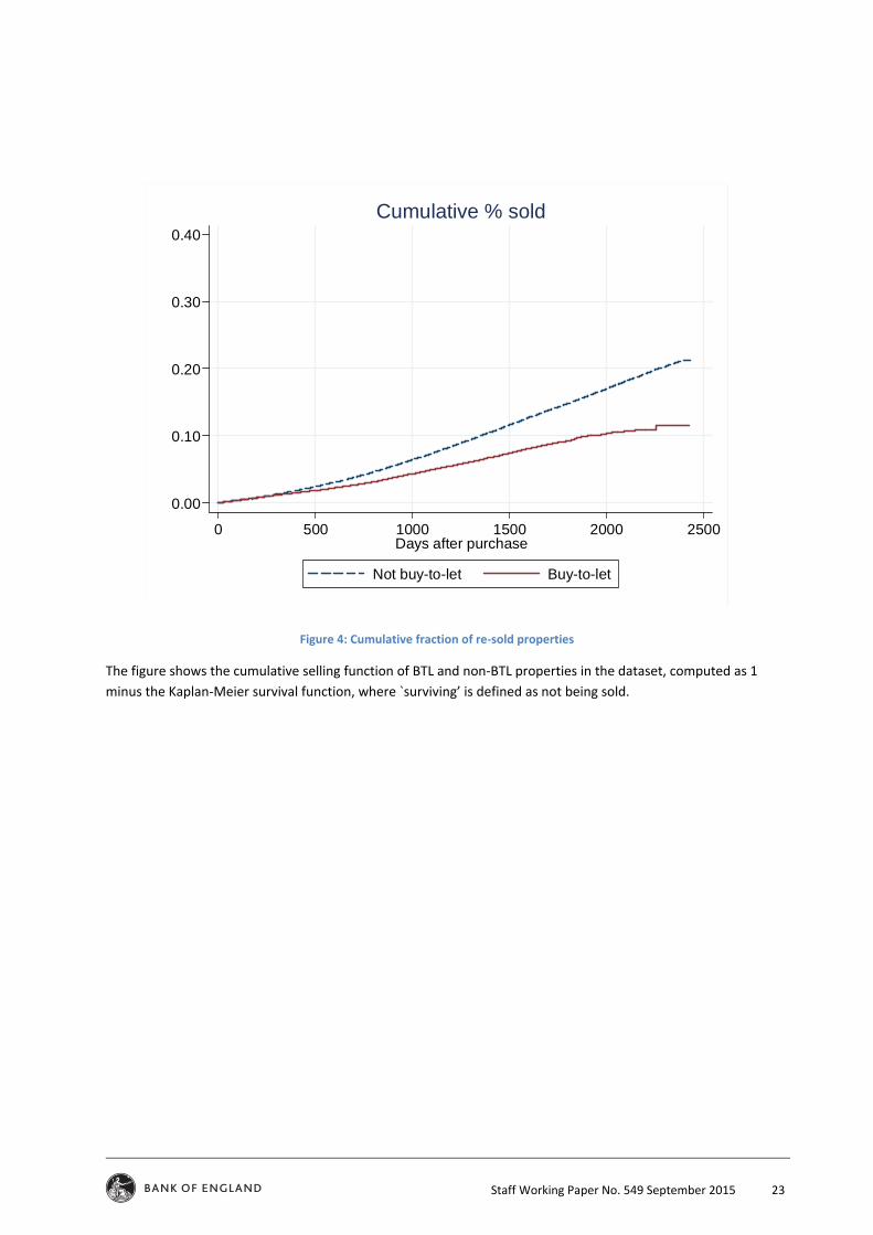
types of buyers, where `surviving’ is defined as not being sold.22 Figure 4 shows the inverse Kaplan‐
Meier functions (i.e. the cumulative selling rate) for the properties in the dataset. Selling rates are
low: only 2% of properties sell twice within 1 year, consistent with the high transaction costs in
England and Wales mentioned in the literature section. The sample is such that we can only track
properties for a maximum of 6 years. This limited time frame is sufficient to notice, in Figure 4, that
the selling rate for BTL properties is actually lower than for other properties.
4 Empiricalanalysis
4.1 TheBTLdiscountThe analysis of the discount associated with BTL purchases is based on hedonic regressions. This
standard technique is employed to control for quality differences between properties and construct
price indices, or estimate the effect of attributes or local conditions on house prices (see Hill, 2013,
for a survey).
The baseline regression has the logarithm of the sale price as dependent variable ( ) and the
available characteristics of the property ( ), the interaction between month of the sale and the
postcode sector ( ), and the listing price ( ) as explanatory variables, plus a BTL indicator:
. 1
The goal of the analysis is to compare BTL purchases with other purchases, making sure that
properties in the two groups are as similar as possible. One confounding factor is that BTL investors
are more likely to buy in specific areas or during specific periods – as shown in the previous Section.
The term controls for these different propensities through time‐location fixed effects.23
Properties in the same area might differ widely in terms of sizes and type of dwelling. The vector
contains the property attributes included in the Land Registry: type of property (whether flat,
terraced, semi‐detached, or detached house), construction period (whether the property is a new
build), and tenure form (freehold or leasehold). It is likely that observable property characteristics do
22 More precisely, I define a `survivor' property at time t a property that was put on the market at time and was not sold at time 1. The cumulative survival function is estimated as
1
where is the number of properties that sold after days, and is the number of properties that were at risk at the beginning of the ‐th day (because they did not sell before and their spell was not censored before ). 23 There are on average 15 units per individual postcode and individual postcodes in the UK have a structure like AB1 2CD. A postcode sector corresponds to all properties which share the “AB1 2” part, i.e. the same postcode district (“AB1”) and a further number. There are approximately 3,000 postcode districts and 10,000 postcode sectors in the UK (see http://en.wikipedia.org/wiki/Postcodes_in_the_United_Kingdom). The empirical strategy is therefore based on high‐dimensional group effects (Gormley and Matsa, 2014).

Staff Working Paper No. 549 September 2015 10
not capture all the property heterogeneity that affects prices. However, most property features that
influence the price are known by the seller, who prices the property accordingly. Therefore, by
including the advertised price for the property, I ensure that these factors are taken into account.
The coefficient represents the percentage effect of BTL on prices once we control for observable
characteristics, advertised prices, month of sale and postcode. This procedure yields an average
effect of BTL in England and Wales over the entire period and for all property types. Standard errors
are computed with two‐way clustering on postcode and time period as described in Petersen (2009).
Table 2 shows the output of the estimation. For the sake of space and clarity, the table does not
display all the coefficients on property characteristics.24 The estimation in the first column uses the
entire LR sample (4m+ sales) and reveals a 10% discount associated with BTL sales. This high
discount leaves open the possibility that the variables included in the regression are not enough to
control for the different property characteristics associated with BTL purchases. Therefore, I restrict
the attention to those properties that at some point were listed on Zoopla either as a rental
property or as a property to be sold. Since Zoopla almost always includes the number of bedrooms
of the property, doing so allows me to have an important control for size. The results are displayed
in the second column of Table 2: the discount associated with BTL purchases declines to 7%. The
contribution of number of bedrooms in terms of explanatory power is apparent in the last row of the
table, which displays the adjusted R‐squared of the regression. Adding bedrooms increases the
adjusted R‐squared by approximately 10 percentage points.
Despite these controls, it is still possible for the BTL coefficient to be biased towards smaller
properties (conditional on number of bedrooms) or properties with lower quality. The third column
of Table 2 shows the results when the regression includes the log listing price without any other
control. The BTL discount is reduced, and is close to half of a percentage point (statistically
significant). Even if the listing price contains all relevant information on the property, the specific
relation between listing and actual price changes according to area, type of dwelling, and time
period (Han and Strange, 2014). Therefore, the fourth column of Table 2 shows a specification
where the listing price enters the regression together with all the controls used previously: dwelling
type, number of bedrooms, and postcode sector‐month dummies. In this case, the discount reaches
1.0%. In a final specification, I restrict the sample of BTL properties to those with a rental Time‐To‐
Market (TTM) up to 3 (rather than 6) months. A property that takes a long time to be advertised for
rent could signal the need for substantial renovation, i.e. low quality. Column 5 of Table 2 shows that
the coefficient on the restricted sample is 0.9%, which may indicate some further correction of the
discount due to a better control for the quality of the property. This reduction in the discount,
however, could also be due to measurement error (more BTL properties are now treated as non‐
BTL) and to investors anticipating some of the renovation costs and managing to obtain a higher
discount than the one owner‐occupiers are able to get for the same property.
24 Results are available on request. All the coefficients have the predicted signs. A new build costs on average 4% more than another property with the same characteristics. A property on a leasehold (as opposed to full freehold ownership) costs 28% less – see Bracke et al (2014) and Giglio et al (2015) for an analysis of the leasehold tenure system in England and its impact on house prices. As expected, detached houses are the most expensive property type, followed by semi‐detached, terraced, and flats.

Staff Working Paper No. 549 September 2015 11
The last two columns of Table 2 form the benchmark result of the paper: everything else equal,
investors spend 0.9‐1.0% less than other buyers. This estimate is likely to be slightly biased towards
zero by the fact that we only identify a fraction of actual BTL purchases – see Appendix C for an
estimate of the bias, which is expected to be around 10% of the measured discount. The Appendix
also contains two robustness checks: a regression where the dependent variable is not the property
sale price but the discount between asking and achieved price25 and an analysis limited to properties
sold in the same postcode sector and month, sharing the same number of bedrooms and the same
asking price.
4.2 HeterogeneityinBTLdiscounts
The regression results presented above reveal the average discount associated to all BTL
transactions. This average could mask quite a diverse distribution; therefore, it is necessary to
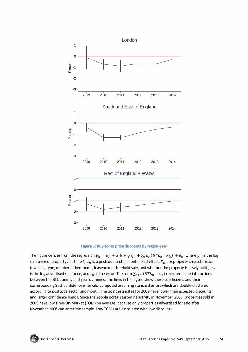
separate out different discounts according to region and year by running the regression:
⋅ ,
where the indicator is interacted with categorical variable . In the main specification of this
part of the paper, corresponds to the interaction of English regions and Wales with year dummies.
Results are displayed in Figure 5.
In London, BTL investors enjoy an average discount of less than 1%, whereas in the South and East of
England discounts are slightly higher, especially in 2010‐2011. In the rest of England and in Wales,
discounts are consistently between 1% and 2%, with a peak of almost 2% in 2010. Comparing these
charts with Figure 3 reveals an inverse relation between the size of the private rented stock (or the
density of BTL activity) and the discount enjoyed by BTL investors. Since regions with large private
rented sectors are also the regions that experienced higher price appreciation over the sample
period (see Appendix Figure A.1), there is an inverse relation between BTL discounts and strength of
the housing market. This relation is explored in more detail in the next subsection, where the
strength of the market is measured as the time needed to sell a house.
In terms of the discounts associated with different years in the sample, the 2009‐2014 period has
been characterised by a recovery of the UK housing market, and correspondingly lower BTL
discounts in all regions and in Wales, as shown in Figure 5.26 Interestingly, in London BTL discounts
are not statistically different from zero in the first part of 2014. Since the current dataset only covers
2014Q1, it will be important to confirm these results once new data sources become available. If
proven correct, these estimates provide the important insight that BTL gradually pay more for
housing, relative to other buyers, as house prices increase.
25 In practice this is equivalent to assuming 1, i.e. a unit elasticity between advertised and actual price. 26 The point estimates for 2009 sit a little outside this pattern, with lower than expected discounts and larger confidence bands. Since the Zoopla portal started its activity in November 2008, properties sold in 2009 have low TOM on average, because only properties advertised for sale after November 2008 can enter the sample. Low TOMs are associated with low discounts.

Staff Working Paper No. 549 September 2015 12
4.3 Marketliquidityanddiscounts
The housing market can be characterised as a search market (Wheaton, 1990); not accepting a
potential buyer’s offer might lead to a longer time waiting for other offers. Selling to an investor at a
discount might be a good idea if it entails a substantial reduction of the Time‐On‐Market (TOM).
To check this hypothesis, I analyse the TOM of properties in the dataset by measuring the distance
between the first appearance of a sale listing and the actual transaction. Figure 6 shows the
distribution of TOMs, expressed in months. The matching procedure delivers a few long TOMs
(above 12 months); in those cases, it is not clear whether the observations are genuine or the
advertisement refers to a previous sale attempt. Therefore, I exclude properties with a TOM longer
than 12 months.27
The first column of Table 3 shows the main coefficients of a regression with the logarithm of TOM as
the dependent variable. The column shows that, consistently with anecdotal evidence, BTL
transactions are associated with a 3% lower TOM. In the data, the average TOM is 5.5 months (see
Figure 6); hence, this discount corresponds to a five‐day reduction. The remaining columns show the
effect of TOM on prices. The coefficient on the logarithm of TOM in Column 2 is ‐3.4%: in general,
properties that stay on the market for longer sell for a lower price. Since properties bought by BTL
investors stay on the market for a shorter period of time, including TOM in the regression does not
change the BTL discount by much. A better way to assess the relation between BTL discount and
TOM is to insert the interaction between these two variables in the regression, as in Column 3. The
negative coefficient signals that BTL are able to extract a higher discount from properties that have
stayed longer on the market, which is consistent with the interpretation of the BTL discount as
compensation for market clearing. The interaction is borderline significant (a coefficient of 0.2% with
a standard error of 0.1%) but the baseline effect of the BTL indicator is reduced to 0.7%. The last
column includes in the regression the interaction of the BTL indicator with the average TOM by
region and year: it may be easier for BTL investors to extract discounts where properties take longer
to sell. This seems to be the case: the insertion of this new term (which is itself not strongly
significant) makes the baseline BTL discount statistically insignificant.
Figure 7 replicates Figure 5 but with TOM as the dependent variable. The data is noisier and
standard errors are larger, but one can notice the same pattern of declining discounts over time.
Also, London discounts are again smaller than those in other regions, especially in 2013 and 2014.
4.4 Mortgagevs.non‐mortgageBTLtransactions
As shown in Table 1, approximately half of BTL transactions are financed with a mortgage, and the
other half are not. The potential differences between these two groups are important because policy
27 As explained in the Data section, there might be several advertisements referring to the same sale. TOM is computed using the first of such advertisements. However, the last advertisement is used to get the listed price used in the regression as control.

Staff Working Paper No. 549 September 2015 13
makers may pay special attention to the mortgage‐financed part of the market. Access to easy credit
has been linked to investor behaviour that is risky for financial stability (Haughworth et al, 2014).
The interpretation of results of this paper would change if the BTL discounts were driven exclusively
by non‐mortgage investors. Table 4 shows that this is not the case. Column 1 illustrates that non‐
mortgage purchases are associated with 5‐6% reduction in TOM – this is expected since non‐
mortgage buyers do not need to go through a bank’s approval to purchase a property. However,
when including this variable, BTL purchases still happen in approximately 2% less time, implying that
all BTL investors, and not only those not funded by mortgages, are quicker at purchasing properties.
Column 2, by including the interaction between BTL and non‐mortgage purchase, demonstrates that
non‐mortgage BTL investors are quicker than the average non‐mortgage buyer. Column 3 shows that
not being financed by a mortgage has virtually no effect on the price paid; the insertion of the
interaction between BTL and non‐mortgage in the last column illustrates that, if anything, BTL non‐
mortgage buyers are likely to pay slightly more than other BTL purchasers (the coefficient is
borderline significant). In fact, while the greater speed of transaction could give a discount to non‐
mortgage transactions, there are arguments which would suggest a positive effect on prices. For
instance, since these purchases are not monitored by a bank, exaggerated prices could be paid. Also,
cash buyers (often recipients of inheritances or pension pots) could be less sophisticated than
professional investors.
Appendix D explores the possibility that BTL discounts are driven by the absence of a chain on the
part of investors, i.e. BTL investors do not need to sell a property before buying a new one, which
reduces uncertainty for the seller. The analysis in the Appendix shows that first‐time buyers, who are
also not tied by a chain, do not enjoy price discounts, which casts doubts on the importance of this
explanation.
5 Conclusion
This paper presents a new way to identify buy‐to‐rent transactions in housing datasets where no
information on buyers and sellers is available. By merging the England and Wales Land Registry with
WhenFresh/Zoopla rental listings, I can spot BTL transactions where a rental listing on a sold
property appears on the web in the 6 months after the sale.
In the descriptive part of the analysis, I show that the identified BTL transactions replicate the time‐
series pattern of aggregate BTL data, although the coverage reaches only one quarter of the total
BTL market. I also show that BTL investors are less likely than other buyers to sell their property in
the six years after the purchase, which confirms that BTL investments are long‐term, different from
short‐term buy‐to‐sell purchases.

Staff Working Paper No. 549 September 2015 14
Comparing properties sold to BTL investors to properties sold to other buyers, this paper
demonstrates that investors enjoy a small but statistically significant discount around 1.0%. When
analysing BTL discounts for different regions and years, I show that discounts are larger when the
housing market is less liquid. BTL discounts are statistically undistinguishable from zero in London at
the end of the sample, when the housing market registered increases in both prices and number of
transactions.
The data show that BTL investors can accelerate the time it takes to sell a property, and BTL
discounts are the implicit compensation for this contribution. However, investors’ ability to `grease
the wheels’ of the housing market becomes limited when the market is already performing well. This
is precisely when financial stability concerns become most important.

Staff Working Paper No. 549 September 2015 15
ReferencesAlbrecht, J, Anderson, A, Smith, E, and Vroman, S (2007) `Opportunistic Matching In The Housing Market’, International Economic Review, 48(2): 641‐664 Anenberg, E and Kung, E (2014). `Estimates of the Size and Source of Price Declines Due to Nearby
Foreclosures’. American Economic Review, 104(8): 2527‐51
Anenberg, E, and Bayer, P (2013). `Endogenous sources of volatility in housing markets: the joint buyer‐seller problem’, NBER Working Paper 18980
Bayer, P, Geissler, C and Roberts, J W (2013). `Speculators and Middlemen: The Role of
Intermediaries in the Housing Market’, Economic Research Initiatives at Duke (ERID) Working Paper
93
Best, M C, and Kleven, H J (2015) `Housing Market Responses to Transaction Taxes: Evidence From Notches and Stimulus in the UK’, unpublished
Bracke, P (2015). `House Prices and Rents: Micro Evidence from a Matched Dataset in Central
London’, Real Estate Economics, 43(2): 403‐431
Bracke, P, Pinchbeck, E W, and Wyatt, J (2014). `The Time Value of Housing: Historical Evidence
from London Residential Leases’, London School of Economics Spatial Economics Research Centre
(SERC) Discussion Paper 168
Chambers, M S, Garriga, C, Schlagenhauf, D (2009a), `Housing policy and the progressivity of income taxation’, Journal of Monetary Economics, 56(8): 1116‐1134
Chambers, M S, Garriga, C, Schlagenhauf, D (2009b) `The loan structure and housing tenure decisions in an equilibrium model of mortgage choice’, Review of Economic Dynamics, 12(3): 444‐468
Chinco, A, and Mayer, C (2014), `Misinformed speculators and mispricing in the housing market’,
NBER Working Paper 19817
Coulson, N E, and Fisher, L M (2012) `Structure and Tenure’, unpublished
Giglio, S, Maggiori, M and Stroebel, J (2015) `Very long‐run discount rates’, Quarterly Journal of Economics, 130(1): 1‐53 Glaeser, E and Shapiro, J (2003) `The Benefits of the Home Mortgage Interest Deduction’ in Tax Policy and the Economy, 17 (J. Poterba, ed.), Cambridge, MA, MIT Press, 37‐82 Gormley, T A, and Matsa, D A (2014) `Common errors: How to (and not to) control for unobserved heterogeneity’, Review of Financial Studies, 27(2):617‐661. Han, L, and Strange, W (2014) `What is the Role of the Asking Price for a House?’, unpublished Haughwout, A, Lee, D, Tracy, J and Van der Klaauw, W (2014) `Real Estate Investors and the
Housing Market Crisis’, unpublished

Staff Working Paper No. 549 September 2015 16
Halket, J and Pignatti, M (2014), `Homeownership and the Scarcity of Rentals’, University of Essex working paper. Hilber, C A, and Lyytikäinen, T (2013). `Housing transfer taxes and household mobility: Distortion on the housing or labour market?’, Government Institute for Economic Research VATT Working Papers 47 Hilber, C A (2005) `Neighborhood externality risk and the homeownership status of properties’, Journal of Urban Economics, 57(2): 213‐241. Hill, R J (2013) `Hedonic price indexes for residential housing: A survey, evaluation and taxonomy’, Journal of Economic Surveys, 27(5), 879‐914. Jones, C, and Richardson, H W (2014) `Housing markets and policy in the UK and the USA: A review of the differential impact of the global housing crisis’, International Journal of Housing Markets and Analysis, 7(1), 129‐144. Kung, E (2015) `The Effect of Credit Availability on House Prices: Evidence from the Economic
Stimulus Act of 2008’, unpublished
Linneman, P (1985) `An economic analysis of the homeownership decision’, Journal of Urban Economics 17 (2): 230‐246. Molloy, R, and Zarutskie, R (2013), `Business Investor Activity in the Single‐Family‐Housing Market’,
Federal Reserve Board of Governors FEDS Notes, December 5
Ngai, L R, and Tenreyro, S (2014) `Hot and Cold Seasons in the Housing Market’, American Economic
Review, 104(12): 3991‐4026.
Petersen, Mitchell A (2009) `Estimating standard errors in finance panel data sets: Comparing
approaches’, Review of Financial Studies, 22(1): 435.
Rosenthal, L (1997), `Chain‐formation in the Owner‐Occupied Housing Market’, The Economic
Journal, 107: 475–488
Sinai, T, and N S Souleles (2005) `Owner‐Occupied Housing as a Hedge Against Rent Risk’, The Quarterly Journal of Economics, 120(2), 763‐789 Smith, M H and Smith, G (2006), `Bubble, Bubble, Where's the Housing Bubble?’, Brookings Papers
on Economic Activity 37 (1): 1‐68.
Wheaton, W C (1990) `Vacancy, Search, and Prices in a Housing Market Matching Model’, Journal of
Political Economy, 98(6): 1270‐1292

Staff Working Paper No. 549 September 2015 17
Appendix
A Regressionswithdiscountsasdependentvariables
Starting from the regression formula in (1), one can assume 1 and move on the other side to
get
,
where is the log difference between the actual price and the advertised price. Table
A.1 shows the results of this exercise. When no controls are included – i.e. we simply compare the
average discount in the market with the average discount of BTL purchases (column 1) – there is no
statistically significant difference between the two. However, BTL investors concentrate on areas
with a strong housing market (as shown in Section 3 of this paper), which are likely to have lower
discounts on average. When the regression contains controls (column 2), the BTL discount becomes
statistically significant at 0.7%. These results are consistent with the discounts shown in the last two
columns of Table 2. Regressions by year, type of property, and region have also been run and have
confirmed the results of the main analysis. Results are available on request.
B Analysisofmatchedrestrictedsample
Given the reliance of regression (1) on postcode sector‐month fixed effects, the identification of a
BTL discount (coefficient ) depends on the presence of postcode sectors where, in the same
months, both a BTL and a non‐BTL purchases took place. A natural robustness check is therefore to
restrict the sample only to those sales that share the same:
‐ postcode sector,
‐ sale month,
‐ property type,
‐ number of bedrooms, and
‐ advertised price.
Moreover, the sets of observations that share the above features must also contain at least one BTL
and one non‐BTL sale. This reduced dataset contains 3772 observations and shows a 1.1% discount
associated with BTL properties, consistent with the regression results.

Staff Working Paper No. 549 September 2015 18
C Econometricconsequencesofbuy‐to‐letmisclassification
Suppose that the true BTL status of a property is given by ∗, whereas the econometrician only
observes , the status derived from matching the England and Wales Land Registry with
WhenFresh/Zoopla listings.
Taking the expectations of equation (1) conditional on the measured (but noisy) status yields
| 1 ∗ Pr ∗ 1| 1 ,
| 0 ∗ Pr ∗ 1| 0 .
The estimated coefficient is equal to
| 1 | 0∗ Pr ∗ 1| 1 Pr ∗ 1| 0 ,
which allows one to evaluate the attenuation bias in . A reasonable assumption is that
Pr ∗ 1| 1 ∼ 1, i.e. sales that are identified as BTL in the sample are true BTL. One
can use aggregate data to estimate Pr ∗ 1| 0 , the likelihood that a true BTL sale is
identified as non‐BTL transaction. According to the Council of Mortgage Lenders, BTL mortgages are
13% of all mortgages. In this paper, BTL transactions are 2.5% of all transactions. Assuming that the
percentage of BTL transactions among cash transactions is the same as the percentage of mortgage
BTL transactions among mortgage transactions, one can say that approximately 10% of all
transactions are misclassified as non‐BTL, i.e. Pr ∗ 1| 0 ∼ 10%. The true ∗ /0.9 = 1.11% if we take the 1.0% estimate as starting point.
D Buy‐to‐letandfirst‐timebuyers
To identify first‐time buyers (FTB) I use the Product Sales Database (PSD), a private dataset collected
by the Financial Conduct Authority (FCA). The PSD has information on UK individual mortgage
transactions since 2005. Only regulated (i.e., homeowner) mortgage contracts are included – other
mortgages, such as BTL loans, are not. The PSD aims at achieving universal coverage of residential
owner‐occupier and only collects information on new sales (mortgages or re‐mortgages), excluding
alterations or top‐ups of the loan. Available variables include mortgage characteristics such as loan
size, length in years, interest rate, and whether the borrower is a FTB. The PSD data is added on top
of the matched dataset through a Land Registry‐PSD probabilistic match based on sale date, price
paid, and complete postcode of the property.
Similarly to BTL investors, FTB do not need to sell a property before they buy a new one. Therefore,
if BTL discounts are due to the absence of these chains, FTB should enjoy them too. This analysis has

Staff Working Paper No. 549 September 2015 19
the added advantage of comparing the behaviour of FTB and BTL purchasers directly – as mentioned
in the introduction, the media often emphasise the role of BTL in `driving out’ FTB from the market.
Columns 1 and 2 of Table A.2 reproduce a couple of regressions of Table 3 adding an indicator for
FTB. The regressions show that FTBs do not enjoy a price discount, despite not being part of a chain,
and properties bought by FTBs spend between 1 and 2% more time on the market. In order to
compare BTL investors and FTBs even more directly, Columns 3 and 4 run the same regressions as
Column 1 and 2 but with a sample composed only by BTL and FTB purchases (dropping the FTB
dummy). Column 3 shows that BTL buyers achieve prices that are more than 1% lower than FTBs.
Column 4 shows that, after controlling for cash purchases, there is no statistically significant
difference between the TOM of properties sold to investors and the TOM of properties sold to FTBs.

Staff Working Paper No. 549 September 2015 20
Figures
Figure 1: Distance in months between buy‐to‐let purchase and WhenFresh/Zoopla rental listing
This histogram uses all sales where a match exists between a Land Registry record and a WhenFresh/Zoopla
rental listing, provided that the Zoopla listing takes place somewhere between 3 months before and 12
months after the sale (which corresponds to month 0 in the chart).
0
10,000
20,000
30,000
40,000
50,000
Sales
-5 0 5 10 15Months

Staff Working Paper No. 549 September 2015 21
Figure 2: Number of buy‐to‐let transactions
The continuous line represents the aggregate number of BTL quarterly mortgages for house purchase in the UK
as reported by the Council of Mortgage Lenders and displayed by the vertical axis on the left. The dashed line
tracks the number of BTL mortgage‐funded sales in the Land Registry‐WhenFresh/Zoopla dataset used by the
paper, and refers to the vertical axis on the right. Notice that the numbers on the right‐hand side axis are
exactly one quarter of the numbers on the left‐hand side axis.
0
1,500
3,000
4,500
6,000
Mat
ched
pro
per
ties
with
mo
rtga
ge
0
6,000
12,000
18,000
24,000
BT
L ad
van
ces
for
hous
e p
urch
ase
2009q1 2010q1 2011q1 2012q1 2013q1 2014q1
CML data (LHS) LR-Zoopla data (RHS)

Staff Working Paper No. 549 September 2015 22
Figure 3: Buy‐to‐let density
The top‐left chart relates the fraction of the stock of housing occupied by private renters in a given region with
the fraction of housing transactions identified as BTL in the Land Registry‐WhenFresh/Zoopla dataset. Data on
the stock of housing and its tenure composition come from the UK Department of Communities and Local
Government. The top‐right chart substitute the regional percentage of private rented stock with the average
regional gross rental yield as computed in the Land Registry‐WhenFresh/Zoopla dataset. The two charts on the
bottom row replicate the analysis of the two top charts by dwelling type rather than region. The bottom‐left
chart shows a positive relation between the percentage of flats that are in private renting with the percentage
of flat sales that are classified as BTL in the Land Registry‐WhenFresh/Zoopla dataset. The bottom‐right chart
has average BTL gross rental yields on the horizontal axis and again shows a positive relation.
North WestYorkshire and The Humber
East of England
London
South East
South West
Wales
North East
East MidlandsWest Midlands
1
2
3
4
5
% B
TL
tra
nsac
tions
, 20
09-2
014
5 10 15 20 25% Private rented stock, 2008
Yorkshire and The Humber
West MidlandsEast of England
London
South East
South West
Wales
North EastEast Midlands
North West
1
2
3
4
5
% B
TL
tra
nsac
tions
, 20
09-2
014
.06 .065 .07 .075Average BTL yield, 2009-2014
detached
flat
semi
terraced
1
2
3
4
5
% B
TL
tra
nsac
tions
, 20
09-2
014
5 10 15 20 25 30% Private rented stock, 2008
detached
flat
semi
terraced
1
2
3
4
5
% B
TL
tra
nsac
tions
, 20
09-2
014
.05 .055 .06 .065 .07Average BTL yield, 2009-2014
Staff Working Paper No. 549 September 2015 23
Figure 4: Cumulative fraction of re‐sold properties
The figure shows the cumulative selling function of BTL and non‐BTL properties in the dataset, computed as 1
minus the Kaplan‐Meier survival function, where `surviving’ is defined as not being sold.
0.00
0.10
0.20
0.30
0.40
0 500 1000 1500 2000 2500Days after purchase
Not buy-to-let Buy-to-let
Cumulative % sold
Staff Working Paper No. 549 September 2015 24
Figure 5: Buy‐to‐let price discounts by region‐year
The figure derives from the regression ∑ ⋅ , where is the log
sale price of property at time , is a postcode sector‐month fixed effect, are property characteristics
(dwelling type, number of bedrooms, leasehold or freehold sale, and whether the property is newly built),
is the log advertised sale price, and is the error. The term ∑ ⋅ represents the interactions
between the BTL dummy and year dummies. The lines in the figure show these coefficients and their
corresponding 95% confidence intervals, computed assuming standard errors which are double‐clustered
according to postcode sector and month. The point estimates for 2009 have lower than expected discounts
and larger confidence bands. Since the Zoopla portal started its activity in November 2008, properties sold in
2009 have low Time‐On‐Market (TOM) on average, because only properties advertised for sale after
November 2008 can enter the sample. Low TOMs are associated with low discounts.
-3
-2
-1
0
1
Pe
rce
nt
2009 2010 2011 2012 2013 2014
London
-3
-2
-1
0
1
Pe
rce
nt
2009 2010 2011 2012 2013 2014
South and East of England
-3
-2
-1
0
1
Per
cen
t
2009 2010 2011 2012 2013 2014
Rest of England + Wales

Staff Working Paper No. 549 September 2015 25
Figure 6: Months between listing and Land Registry sale
By merging the Land Registry with WhenFresh/Zoopla sale listings, it is possible to compute the distance
between the month in which the listing went online and the month when the sale was completed (as recorded
by the Land Registry). The maximum distance is limited to 12 months to avoid instances where the
advertisement and the actual transaction do not correspond to the same sale event (for example, when the
property was first listed and then withdrawn, then listed again). The histogram shows these distances in
months, and the vertical axis reports the number of sales that fall in a given category.
0
50,000
100,000
150,000
200,000
250,000
Sales
0 5 10 15Months

Staff Working Paper No. 549 September 2015 26
Figure 7: Buy‐to‐let time‐on‐market (TOM) discounts by region‐year
The figure derives from the regression ∑ ⋅ , where is the log
TOM of property at time , is a postcode sector‐month fixed effect, are property characteristics
(dwelling type, number of bedrooms, leasehold or freehold sale, and whether the property is newly built),
is the log advertised sale price, and is the error. The term ∑ ⋅ represents the interactions
between the BTL and year dummies. The lines in the figure show these coefficients and their corresponding
95% confidence intervals, computed assuming standard errors which are double‐clustered according to
postcode sector and month.
-10
-5
0
5
Per
cent
2009 2010 2011 2012 2013 2014
London
-10
-5
0
5
Per
cent
2009 2010 2011 2012 2013 2014
South and East of England
-10
-5
0
5
Per
cent
2009 2010 2011 2012 2013 2014
Rest of England + Wales

Staff Working Paper No. 549 September 2015 27
Figure A.1: Regional house price indices, 2007‐2015
The indices are nominal and taken from the Land Registry website (http://landregistry.data.gov.uk/app/hpi/)
and normalised so that the 2007 peak corresponds to 100. The first row includes London alone with its unique
price increase. The second group of regions, corresponding to the second row in the Figure, includes regions
whose nominal prices are either above or very close to the 2007 peak. The last two rows contain the remaining
English regions and Wales.
8090
100
110
120
130
2007 2009 2011 2013 2015
London80
8590
9510
010
5
2007 2009 2011 2013 2015
South East80
8590
9510
0
2007 2009 2011 2013 2015
South West
8085
9095
100
105
2007 2009 2011 2013 2015
East
7580
8590
9510
0
2007 2009 2011 2013 2015
North East
7580
8590
9510
0
2007 2009 2011 2013 2015
North West80
8590
9510
0
2007 2009 2011 2013 2015
Wales
8085
9095
100
2007 2009 2011 2013 2015
East Midlands
8085
9095
100
2007 2009 2011 2013 2015
Yorkshire and Humber
8085
9095
100
2007 2009 2011 2013 2015
West Midlands

Staff Working Paper No. 549 September 2015 28
Tables
Land Registry (Sales)
WhenFresh/Zoopla (Rentals)
Matched (BTL)
Observations 4,014,482 3,749,509 100,669
Median price (rent) 177,000 179 150,000
Flat 0.19 0.46 0.30
Terraced 0.28 0.24 0.38
Semi 0.29 0.14 0.22
Detached 0.24 0.09 0.08
Other 0.06
Lease 0.24 0.34
Mortgage 0.68 0.53
New 0.10 0.04
Table 1: Descriptive statistics, main data sources
The first two columns show data from two of the original data sources used in this paper, the England and
Wales Land Registry and WhenFresh/Zoopla rental listings. The third column shows data from the subset of
BTL matched properties, i.e. properties that have both a Land Registry sale and a WhenFresh/Zoopla rental
listing, and the distance between the two does not exceed 6 months. To avoid outliers or wrongly‐typed
observation to influence the results, the bottom and the top percentile in terms of prices, rents, and yields
have been removed from the data.

Staff Working Paper No. 549 September 2015 29
(1) (2) (3) (4) (5) Log Price Log Price Log Price Log Price Log price
BTL purchase ‐0.103 ‐0.070 ‐0.004 ‐0.010 (0.002) (0.001) (0.001) (0.001) Log listing price 1.009 0.980 0.980 (0.001) (0.001) (0.001) BTL purchase ‐0.009 (TTM = 3 months) (0.001) Land Reg Controls YES YES YES YES Bedrooms YES YES YES Pcode sector‐month YES YES YES YES
Observations 3,956,591 2,494,075 1,294,312 1,276,065 1,276,065 Adj. R2 0.69 0.80 0.99 0.99 0.99
Table 2: Hedonic regression for the effect of buy‐to‐let on prices
The table shows results from the regression , where is the log sale
price of property at time , is a postcode sector‐month fixed effect, are property characteristics (Land
Registry controls: dwelling type, leasehold or freehold sale, and whether the property is newly built;
WhenFresh/Zoopla information: number of bedrooms), is the log advertised sale price, is a dummy
that indicates whether the sale has been identified as a BTL purchase, and is the error. The regression is run
with double‐clustered (according to postcode sector and month) standard errors, shown in parentheses.
Column 5 restricts the definition of BTL to sales where the distance from the rental listing does not exceed 3
months (instead of 6 months as in the rest of the paper).

Staff Working Paper No. 549 September 2015 30
(1) (2) (3) (4) Log TOM Log Price Log Price Log Price
BTL purchase ‐0.029 ‐0.011 ‐0.007 0.008 (0.004) (0.004) (0.001) (0.013) Log TOM ‐0.034 ‐0.034 ‐0.034 (0.001) (0.001) (0.001) BTL * Log TOM ‐0.002 ‐0.002 (0.001) (0.001) BTL * Log Regional TOM ‐0.009 (0.007) Log listing price YES YES YES YES Land Reg Controls YES YES YES YES Bedrooms YES YES YES YES Pcode sector‐month YES YES YES YES
Observations 1,260,027 1,260,027 1,260,027 1,260,027 Adj. R2 0.15 0.99 0.99 0.99
Table 3: Time‐On‐Market (TOM) regressions
The first column of the table reports results from regressions analogous to the one in Table 2, but where the
logarithm of the sale Time‐On‐Market (TOM) is the dependent variable: log
. Columns 2 and 3 show the usual regression with the logarithm of the sale price as the
dependent variables, but including log TOM as an explanatory variable (Column 2), and also its interaction with
(Column 3). The last column also includes a measure of the average TOM in the regional and year when
the sale took place. Other regression controls and standard errors are as described in the caption of Table 2.
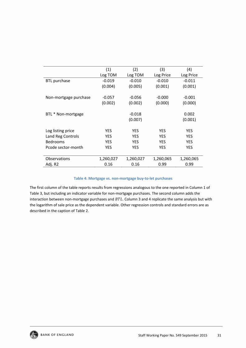
Staff Working Paper No. 549 September 2015 31
(1) (2) (3) (4) Log TOM Log TOM Log Price Log Price
BTL purchase ‐0.019 ‐0.010 ‐0.010 ‐0.011 (0.004) (0.005) (0.001) (0.001) Non‐mortgage purchase ‐0.057 ‐0.056 ‐0.000 ‐0.001 (0.002) (0.002) (0.000) (0.000) BTL * Non‐mortgage ‐0.018 0.002 (0.007) (0.001) Log listing price YES YES YES YES Land Reg Controls YES YES YES YES Bedrooms YES YES YES YES Pcode sector‐month YES YES YES YES
Observations 1,260,027 1,260,027 1,260,065 1,260,065 Adj. R2 0.16 0.16 0.99 0.99
Table 4: Mortgage vs. non‐mortgage buy‐to‐let purchases
The first column of the table reports results from regressions analogous to the one reported in Column 1 of
Table 3, but including an indicator variable for non‐mortgage purchases. The second column adds the
interaction between non‐mortgage purchases and . Column 3 and 4 replicate the same analysis but with
the logarithm of sale price as the dependent variable. Other regression controls and standard errors are as
described in the caption of Table 2.

Staff Working Paper No. 549 September 2015 32
(1) (2) Log Discount Log Discount
BTL purchase ‐0.002 ‐0.007 (0.001) (0.001) Land Reg Controls YES Bedrooms YES Pcode sector‐month YES
Observations 1,583,225 1,560,640 Adj. R2 0.00 0.15
Table A.1: Hedonic regression for the effect of buy‐to‐let on the asking price discount
The table reports results from the regression , where is the
difference, in logarithms, between the actual price and the advertised price of a sold property. The two
columns in the table replicate columns 3 and 4 of Table 2, but assuming a coefficient of 1 on the advertised
sale price. Other regression controls and standard errors are as described in the caption of Table 2.

Staff Working Paper No. 549 September 2015 33
(1) (2) (3) (4) All sales BTL and FTB only Log Price Log TOM Log Price Log TOM
BTL purchase ‐0.011 0.008 ‐0.013 ‐0.004 (0.001) (0.005) (0.001) (0.010) Non‐mortgage purchase 0.001 ‐0.070 0.001 ‐0.075 (0.001) (0.007) (0.001) (0.012) First Time Buyer 0.001 0.019 (0.000) (0.003) Log listing price YES YES YES YES Land Reg Controls YES YES YES YES Bedrooms YES YES YES YES Pcode sector‐month YES YES YES YES
Observations 1,276,065 1,260,027 253,131 252,118 Adj. R2 0.99 0.15 0.99 0.17
Table A.2: Hedonic and Time‐On‐Market regressions, buy‐to‐let vs. first‐time buyers
This table shows regression results that include information on whether a given sale was purchased by a First
Time Buyer (FTB). The first column replicates the last column of Table 2 but includes the non‐mortgage dummy
and the FTB dummy. The second column reports the same regression but with the logarithm of TOM as the
dependent variable. The third and fourth columns also present results from a regression on log sale price and a
regression on log TOM; in this case, however, the sample is limited to BTL and FTB purchases to allow a more
direct comparison between the two. Other regression controls and standard errors are as described in the
caption of Table 2.