Bank of Canada Banque du Canada

Working Paper 97-16 / Document de travail 97-16

Canadian Policy Analysis Model: CPAM

by

Richard Black and David Rose

ISSN 1192-5434ISBN 0-662-26005-8

Printed in Canada on recycled paper

Bank of Canada Working Paper 97-16

June 1997

Canadian Policy Analysis Model: CPAM

by

Richard Black

Research Department,Bank of Canada, Ottawa, K1A 0G9

Tel: (613) 782-8399; Fax: 613) 782-8334E-mail: rblack@bank-banque-canada.ca

and

David Rose

QED SOLUTIONS,248 Queen Elizabeth Drive, Ottawa, K1S 3M5

Tel: (613) 231-7846; Fax: (613) 231-6771E-mail: drose@cyberus.ca

The views expressed in this paper are those of the authors and QED SOLUTIONS.No responsibility for them should be attributed to the Bank of Canada.

Acknowledgments

This work builds on other modelling work done at QED SOLUTIONS for the Reserve

Bank of New Zealand. We thank Enzo Cassino, Aaron Drew, Eric Hansen, Ben Hunt,

David Mayes, and Alasdair Scott for their questions and comments. We also thank

participants in a seminar at the Bank of Canada for their input, particularly David

Longworth, Tiff Macklem, and Simon van Norden. Any errors are our responsibility.

Abstract

This paper documents the structure and properties of the Canadian Policy Analysis Model

(CPAM). CPAM is designed to provide a reasonably complete representation of the Canadian

macro economy. It is a one-domestic-good, small-open-economy model, which features an

endogenous supply side, behavioural equations for the principal components of demand, forward-

looking expectations, and reaction functions for both the monetary and fiscal authorities. The

model has an explicit steady state and is dynamically stable over a wide range of disturbances.

CPAM is similar in many ways to the Bank of Canada's Quarterly Projection Model (QPM), and it

has been calibrated to reflect QPM's dynamic properties in deterministic simulations. CPAM is

smaller, however, and has been configured to simulate much faster than QPM so that stochastic

simulations on a large scale are feasible.

Résumé

Les auteurs exposent la structure et les propriétés du Modèle d’analyse des politiques

(MAP), qui a été conçu pour représenter assez fidèlement l’ensemble de l’économie canadienne.

Le modèle décrit une petite économie ouverte qui ne produit qu’un seul bien et où l’offre est

endogène et les attentes prospectives. Il comporte des équations formalisant le comportement des

principales composantes de la demande ainsi que des fonctions de réaction propres aux autorités

monétaires et budgétaires. Il englobe un régime permanent explicite, et sa structure dynamique est

stable pour un large éventail de chocs. Le MAP ressemble à de nombreux égards au Modèle

trimestriel de prévision (MTP) de la Banque du Canada, et son étalonnage reflète les propriétés

dynamiques affichées par le MTP dans le cadre de simulations déterministes. Le MAP est toutefois

plus petit et, comme il se résoud bien plus rapidement que le MTP, il permet des simulations

stochastiques à grande échelle.

Contents

1. Introduction. .. . . . . . . . . . . . . . . . . . . . . . . . . . . . . . . . . . . . . . . . . . . . . . . . . . . . . . 1

2. The structure of CPAM. . . . . . . . . . . . . . . . . . . . . . . . . . . . . . . . . . . . . . . . . . . . . . 42.1 Notation and measurement conventions . . . . . . . . . . . . . . . . . . . . . . . . . . . 42.2 Growth accounting assumptions . . . . . . . . . . . . . . . . . . . . . . . . . . . . . . . . . 52.3 Expenditure accounts . . . . . . . . . . . . . . . . . . . . . . . . . . . . . . . . . . . . . . . . . 6

2.3.1 The GDP identies . . . . . . . . . . . . . . . . . . . . . . . . . . . . . . . . . . . . . . 62.4 Consumption . . . . . . . . . . . . . . . . . . . . . . . . . . . . . . . . . . . . . . . . . . . . . . . 7

2.4.1 Adjustment dynamics . . . . . . . . . . . . . . . . . . . . . . . . . . . . . . . . . . . 82.4.2 Equilibrium consumption and wealth . . . . . . . . . . . . . . . . . . . . . . . 9

2.5 Investment . . . . . . . . . . . . . . . . . . . . . . . . . . . . . . . . . . . . . . . . . . . . . . . . . 102.6 Government expenditure and transfers . . . . . . . . . . . . . . . . . . . . . . . . . . . 112.7 External trade . . . . . . . . . . . . . . . . . . . . . . . . . . . . . . . . . . . . . . . . . . . . . . 11

2.7.1 Imports . . . . . . . . . . . . . . . . . . . . . . . . . . . . . . . . . . . . . . . . . . . . . 112.7.2 Exports . . . . . . . . . . . . . . . . . . . . . . . . . . . . . . . . . . . . . . . . . . . . . 132.7.3 Trade balance identities . . . . . . . . . . . . . . . . . . . . . . . . . . . . . . . . 14

2.8 Income accounts . . . . . . . . . . . . . . . . . . . . . . . . . . . . . . . . . . . . . . . . . . . . 142.8.1 Wages . . . . . . . . . . . . . . . . . . . . . . . . . . . . . . . . . . . . . . . . . . . . . . 142.8.2 Labour income . . . . . . . . . . . . . . . . . . . . . . . . . . . . . . . . . . . . . . . 152.8.3 Risk income . . . . . . . . . . . . . . . . . . . . . . . . . . . . . . . . . . . . . . . . . 16

2.9 Capital stock and user cost of capital . . . . . . . . . . . . . . . . . . . . . . . . . . . . 172.10 The government budget constraint: bonds and taxes . . . . . . . . . . . . . . . . 172.11 Net foreign assets and the remaining asset identities . . . . . . . . . . . . . . . . 182.12 Supply . . . . . . . . . . . . . . . . . . . . . . . . . . . . . . . . . . . . . . . . . . . . . . . . . . . . 19

2.12.1 Employment . . . . . . . . . . . . . . . . . . . . . . . . . . . . . . . . . . . . . . . . . 192.12.2 Total factor productivity . . . . . . . . . . . . . . . . . . . . . . . . . . . . . . . . 192.12.3 Equilibrium and potential output . . . . . . . . . . . . . . . . . . . . . . . . . 19

2.13 The monetary nexus . . . . . . . . . . . . . . . . . . . . . . . . . . . . . . . . . . . . . . . . . 202.13.1 The reaction function . . . . . . . . . . . . . . . . . . . . . . . . . . . . . . . . . . 202.13.2 The term structure of interest rates . . . . . . . . . . . . . . . . . . . . . . . . 212.13.3 Links to world rates and “risk” premia . . . . . . . . . . . . . . . . . . . . . 22

2.14 Exchange rate dynamics . . . . . . . . . . . . . . . . . . . . . . . . . . . . . . . . . . . . . . 222.15 Inflation. . . . . . . . . . . . . . . . . . . . . . . . . . . . . . . . . . . . . . . . . . . . . . . . . . . . 23

2.15.1 The Phillips curve . . . . . . . . . . . . . . . . . . . . . . . . . . . . . . . . . . . . . 232.15.2 Expectations . . . . . . . . . . . . . . . . . . . . . . . . . . . . . . . . . . . . . . . . . 25

2.16 Relative prices. . . . . . . . . . . . . . . . . . . . . . . . . . . . . . . . . . . . . . . . . . . . . . 272.16.1 Foreign relative prices . . . . . . . . . . . . . . . . . . . . . . . . . . . . . . . . . 30

2.17 Calibration equations and output transforms . . . . . . . . . . . . . . . . . . . . . . 312.17.1 Calibration equations . . . . . . . . . . . . . . . . . . . . . . . . . . . . . . . . . . 312.17.2 The postcom macro. . . . . . . . . . . . . . . . . . . . . . . . . . . . . . . . . . . . 32

3. The dynamic properties of CPAM . . . . . . . . . . . . . . . . . . . . . . . . . . . . . . . . . . . . 343.1 A temporary demand shock . . . . . . . . . . . . . . . . . . . . . . . . . . . . . . . . . . . 343.2 A temporary exchange rate shock. . . . . . . . . . . . . . . . . . . . . . . . . . . . . . . 363.3 A temporary tightening in monetary conditions . . . . . . . . . . . . . . . . . . . . 383.4 A temporary increase in inflation . . . . . . . . . . . . . . . . . . . . . . . . . . . . . . . 403.5 An increase in world commodity prices . . . . . . . . . . . . . . . . . . . . . . . . . . 423.6 An increase in total factor productivity. . . . . . . . . . . . . . . . . . . . . . . . . . . 443.7 A change in the target rate of inflation . . . . . . . . . . . . . . . . . . . . . . . . . . . 463.8 A permanent change in government debt . . . . . . . . . . . . . . . . . . . . . . . . . 48

Contents(continued)

Appendix A: The adjustment mechanism in CPAM. . . . . . . . . . . . . . . . . . . . . . . . . . . . . 50Appendix B: Mnemonics, descriptions, and values . . . . . . . . . . . . . . . . . . . . . . . . . . . . . 53References. . .. . . . . . .. . . . . . . . . . . . . . . . . . . . . . . . . . . . . . . . . . . . . . . . . . . . . . . . . . . . . 66

1

1. Introduction

This paper documents the structure and properties of a model designed for stochastic

simulation analysis of the Canadian economy and, in particular, issues facing the monetary

authority in implementing a nominal anchor for the economy. This model, dubbed CPAM, for

Canadian Policy Analysis Model, is based on a family of models developed by QED

SOLUTIONS.1

CPAM, which has quarterly frequency, is designed to provide a reasonably complete

representation of the Canadian macro economy. It is a one-domestic-good, small-open-economy

model, which features an endogenous supply side, behavioural equations for the principal

components of demand, forward-looking expectations, and reaction functions for both the

monetary and fiscal authorities. The model has an explicit steady state and is dynamically stable

over a wide range of disturbances. CPAM has about 140 equations, of which perhaps 30 describe

the essential agent behaviour. It has many features similar to the Bank of Canada’s Quarterly

Projection Model (QPM), including the same core theory of household behaviour, and it has been

calibrated to reflect current Bank of Canada staff judgments regarding exogenous variables, the

numerical steady-state solution, and many features of dynamic properties in deterministic

simulations.2 CPAM is smaller, however, and has been configured to simulate much faster than

QPM so that stochastic simulations on a large scale are feasible.3 Indeed, it was this desire to make

stochastic simulations a practical tool for policy analysis that provided the central motivation for

building CAPM. See Black, Macklem, and Rose (1997) for a first application of stochastic

simulations with CPAM to consider alternative monetary-policy reaction functions for price

stability.

There are three domestic sectors: households, firms, and a consolidated government. There

is no formal financial sector. Households own capital directly; they also hold the bonds issued by

the government and (reflecting the Canadian case) they have liabilities to foreigners. The steady

1. CPAM was prepared for the Bank of Canada under a research contract with David Rose of QEDSOLUTIONS. CPAM exploits some of the structure and methodology developed in the construction of amodel of the New Zealand economy for the Reserve Bank of New Zealand. A Reserve Bank publication onthe new Forecasting and Policy System (FPS) is forthcoming.

2. For details on the structure and properties of QPM see Black, Laxton, Rose, and Tetlow (1994) and Coletti,Hunt, Rose, and Tetlow (1996). An overview is available in Poloz, Rose, and Tetlow (1994).

3. The difference in simulation times is at least a factor of 5.

2

state describes an equilibrium of a small open economy with stable ratios of each of these stocks to

output.

Fiscal policy is characterized as choices about the debt-to-output and expenditure-to-output

ratios; the rate of personal direct taxation is used as the instrument for fiscal closure (respecting the

intertemporal budget constraint). Monetary policy is characterized as the choice of a target rate of

inflation. This is implemented through a forward-looking reaction function, in which the monetary

authority acts on the short-term interest rate according to where inflation is predicted to be, relative

to the target rate, 7 to 8 quarters ahead.

There are some differences between CPAM and QPM. An important difference concerns

the accounting and modelling structure for prices. QPM abandons the logic of the one-domestic-

good paradigm to permit an independent Phillips curve for the CPI excluding food and energy.

CPAM sticks more closely to the internal logic of the one-good paradigm. A core domestic price,

the domestic aborption deflator at factor cost, PDFC, is treated as both the numeraire for the

accounts and the fundamentally stochastic domestic price.4 We choose PDFC as the core price,

since it represents the average revenue received by firms on final sales into the domestic market,

which is as close as we can get to a quintessentially domestic price. It is also the price that is most

closely linked, in principle, to domestic costs.

All other price indexes are built from this core price and trade prices. Thus, for example, the

consumption good price in the model comes from a weighted combination of the import price and

the domestic core price for consumption goods, all appropriately adjusted for taxes, using the

model’s accounting identity structure. In particular, the endogenous share of imported consumption

goods provides the weight for the import price in the index.

The Phillips curve in CPAM relates core inflation to domestic demand conditions and some

other dynamic factors. But the monetary authority is concerned with the outcome for consumer

price inflation. This means that the effect of monetary intervention on import prices through the

exchange rate plays an important role in the transmission mechanism and in inflation dynamics

generally.

4. The domestic absorption deflator is defined as follows: Domestic absorption is simply what is produced andnot exported:YD = Y-X. The absorption deflator is then given implicitly fromPY*Y=PD*YD+PX*X. This isat market. To get the measure at factor cost, we must remove the direct effect of indirect taxes:PD*YD=PDFC*YD+indirect taxes.

3

Another important difference between CPAM and QPM is in the modelling of dynamics.

QPM expresses many adjustment processes using error-correction mechanisms based on the gap

between the current value and the steady-state value of a variable. In many cases, however,

especially in those shocks where the initial adjustment must be contrary to the steady-state effect,

as in most cases where there is a change in the net foreign asset (NFA) position, QPM is forced to

rely on other special terms to generate the appropriate short-term response. In CPAM, we exploit

the underlying theory to a greater degree, building into what we call the “equilibrium” values of the

endogenous variables this important distinction between the equilibrium transition path and the full

steady-state effects. Thus, CPAM dynamics have an extra layer not developed in QPM. Much of

what QPM represents as pure disequilibrium effects, appears in CPAM as “equilibrium dynamics.”

This enables us to make a much clearer distinction as to why “perverse” short-term movements

often arise in scenarios with asset adjustment as a central feature.

Some differences between CPAM and QPM are more style than substance. For example,

CPAM is written using Euler equations rather than QPM’s explicit solutions in terms of expected

future values. An advantage of the CPAM representation is that the equations are much more

compact and easier to report. Indeed,all of the equations of CPAM are presented and described in

this document. The model itself is also more compact, because explicit equations for all the future

leads within the expectations structures are not required.5

The rest of the paper is organized as follows. In Section 2, we document the complete

structure of CPAM. The model equations are reported using TROLL syntax, exactly as they appear

in the simulation code. Appendix B provides extra details, including a complete list of all model

mnemonics and definitions, the parameter values, the exogenous variable assumptions, and the

other inputs into the steady-state solution, as well as that steady-state solution itself. Section 3

describes CPAM’s dynamic properties through the results of deterministic simulations of the

model’s response to a number of standard shocks.

5. This means that CPAM does not need the macro for generating expectations that is relied on heavily in QPM.The same thing is achieved within TROLL in the stacking procedure used in the simulation algorithm.Armstrong, Black, Laxton, and Rose (1995) discuss this method.

4

2. The structure of CPAM

We now turn to a detailed review of the equations of CPAM. We first review a few points

of notation, TROLL syntax, and our measurement conventions, which are necessary background to

understanding what follows. We then describe the model equations. The discussion is broken into

sections in a relatively standard way, but with a few minor exceptions, the whole system is

simultaneous.

2.1 Notation and measurement conventions

Variables with a suffix.eq are dynamic equilibrium values. The equilibrium values will

converge on steady-state (SS) values. However, the.eq values differ, in principle, from the SS

values when the model is shocked. Only in special cases will these equilibrium values be identical

to the steady-state values in the immediate aftermath of a shock. CPAM exploits this information

in modelling the dynamics.

All real variables in CPAM are measured relative to a trend that grows at the SS growth rate

of output. In the control solution, the level of output has also been normalized to 1 (annual rates) in

some notional base period. Thus, for example, all the annual rate GDP components are fractions—

shares of output—in the control solution. Nominal variables are also divided by the domestic

absorption deflator, measured at factor cost. In other words, every price in the core model is a

relative price. Also, for the steady state, no trends are permitted in shares or relative prices, so all

variables have particular numerical solutions. The SS numbers are computed from a solution of the

model with leads and lags eliminated. The ease of this procedure is one advantage of writing the

model in detrended form. Trend real and nominal growth are reintroduced in a separate component

(a TROLL macro we call “postcom”) that converts the core model variables to more familiar units.

The core model is written with all variables in their natural quarterly units. Thus, for

example, all expenditure flows are at quarterly rates. Similarly, all growth rates, inflation rates, and

interest rates are measured quarterly at quarterly rates. Under these conventions, model equations

are almost void of code that merely converts units. For studying model output, however, annual

rates are often more convenient. The postcom macro provides all the necessary transforms. A

variable with prefixa, with underscore, as ina_x, is the annualized version of the variablex. In the

case of flows, this is just multiplying by 4. In the case of rates etc., the calculation includes the effect

of compounding. Thus, for example, the quarterly-at-annual-rate measure of inflation,a_pdot, is

5

derived from (1+a_pdot) = (1+pdot)**4. Another feature is level transforms. When growth and

inflation are added to the model solution, variables with prefixl_ are created, where appropriate.

Thus, one can see the solution for the level of the GDP deflator in the variablel_py.

As indicated above, the equations are reported in TROLL format. In TROLL syntax,x(J) is

the Jth lead ofx, and for an endogenous variable in a deterministic simulation this will be the model

solution J periods ahead. Similarly,x(-J) is the Jth lag ofx. CPAM uses very few functions or other

special operators. Where necessary, these are described with the equation.

The only other feature of TROLL syntax that is necessary for what follows is the labelling

convention for equations. Each equation begins with a label, followed by a colon. Then comes the

actual equation. It should go without saying, but just to be safe we will say it, labels are arbitrary

in a simultaneous system. The entireN equations of a non-singular system determineN unknowns.

Yet some economists persist in wanting to label everything as if this were not true and the model

could be considered as a set of reduced-form equations. We use the phrase “proximately determine”

when describing some equations to identify the variable that has conventionally been used as the

notional “dependent” variable in such discussions, based on recursive solution methods, like

Gauss-Seidel. In TROLL, it is the endogenous variable list that matters. Derivatives are taken for

all equations with respect to all endogenous variables. Equations do not have to be written in a form

already normalized on a particular variable. In fact, the label can be a variable that does not appear

in the equation; there are several examples in CPAM. The labels are not actually used for anything

real. Hence, they do not even have to be variable names. Of course, it is still necessary to haveN

equations to solve forN unknowns, and there is nothing wrong with using the names of the

endogenous variables as labels—there are just the right number, after all. Essentially, that is what

we have done.

2.2 Growth accounting assumptions

Trend population growth,ndot, and trend productivity growth,qdot,which is measured in

labour units, are exogenous. In this version of the model, there are no variations in these trend

values through time. Actual productivity growth, measured as the percentage change in the level of

total factor productivity, say,will vary with the cycle. Overall trend real growth,ydot, is defined

from the components, as required by the underlying neoclassical growth model:

(1) ydot: ydot =(1+ndot)*(1+qdot) - 1.

6

Again, this is a trend growth concept and is essentially exogenous. It isnot the growth rate in actual

output period-by-period. That, of course, is endogenous to the model. The numerical assumptions

for steady-state growth are taken from QPM (labour-embodied technical progress at 1.3 per cent

per annum and population growth at just under 0.95 per cent per annum, for a trend growth in

potential output of about 2.25 per cent per annum).

2.3 Expenditure accounts

The standard expenditure add-up identities are included, but with two twists, as alluded to

previously. The first is our detrending procedure. Thus model variabley is not constant-dollar

output. If Y is the constant-dollar measure at annual rates, it is rescaled according toy(t)=Y(t)/

(4*Y0*(1+ydot)**t), whereY0 is the annual-rate value in a base period (i.e., we also normalize the

control annual-rate value ofy to be 1 and the quarterly rate value to be 0.25). The same rescaling is

carried out forc, i, etc. Thus, the control levels of components of spending are their proportional

shares of output.

The second twist is that the prices are not the national accounts deflators. Rather, all prices

are measured relative to the numeraire price, which we take to be the domestic absorption deflator

at factor cost (PDFC). Indirect taxes are levied on consumption, investment, and government

goods, at effective rates taken from QPM.

As in QPM, the sectoral accounting framework is simplified. In particular, residential

investment and changes in the stock of inventories are notionally included in model “consumption.”

2.3.1 The GDP identities

In current terms, we have:6

(2) y: y = c + i + g + x - m,

(3) py: py*y = pc*c + pk*i + pg*g + px*x - pm*m.

In .eq terms we have:

(4) py.eq: y.eq = c.eq + i.eq + g.eq + x.eq - m.eq.

Note that this is an example of an equation with a label given by a variable that does not appear in

the equation itself. We think ofy.eq as being proximately determined by the supply side of the

6. We use the seemingly inconsistent mnemonicpk for the flow investment price simply because one of thesoftware packages we use for applications reserves the mnemonicpi for the mathematical constant.

7

model. This equilibrium condition, which imposes the requirement that supply must equal demand,

then proximately determines the equilibrium price.

Next comes the identity for the average price at factor cost:

(5) pfc: py*y = pfc*y + tic*pc*c/(1+tic)

+tii*pk*i/ (1+tii) +tig*pg*g/ (1+tig),

wheretic, tii, and tig are the rates of indirect tax on consumption, investment, and government

purchases, all measured net of any subsidies. The terms involving these variables together reflect

net indirect tax revenues. We have the same structure in.eq terms:

(6) pfc.eq: py.eq*y.eq = pfc.eq*y.eq + tic*pc.eq*c.eq/(1+tic)

+ tii*pk.eq*i.eq/(1+tii) +tig*pg.eq*g.eq/(1+tig),

The final equation in this block is a check that the equilibrium model satisfies the GDP

identity. Note that, for reasons we explain later, the variablecheck1, which must be identically zero

if the identity holds, appears later in the model—in the risk income equation. But it can be thought

of as the balancing entry for this identity.

(7) check1: py.eq*y.eq = pc.eq*c.eq + pk.eq*i.eq + pg.eq*g.eq

+ px.eq*x.eq - pm.eq*m.eq.

2.4 Consumption

There are two kinds of consumers in CPAM. There are forward-looking agents, who make

decisions with a view to picking the best path for current and future consumption. Their choices are

shown in variables with “fl” in the mnemonic. Thuscfl is consumption by forward-looking agents.

CPAM also has agents who consume by the simple “rule of thumb” (rt) that they consume what

they receive in income every period. Thus, all assets are held by the forward-looking agents. Total

consumption,c, is the sum of the demands from the two types of agent.

(8) c: c = crt + cfl.

Section 2.8.2 describes how disposable income is divided between the two types of agents.

8

2.4.1 Adjustment dynamics

RT consumers just use up their real disposable income,ydrt. Note that the left side isnota

current dollar expression;pc is a relative price (the consumption price divided by PDFC). Thuspc

here simply converts the real units to be consistent.

(9) crt: pc*crt = ydrt.

The next equation contains the consumption dynamics for the forward-looking agents. The

structure of the equation is typical of those in the rest of the model. It says that consumption (of

forward-looking agents),cfl, will converge on its equilibrium value,cfl.eq, subject to an adjustment

structure, provided through the variablecfladj, as well as to the influence of a number of special

disequilibrium effects.

(10) cfl: cfl = cfl.eq + cv1*(ydfl(-2)/pc(-2)-ydfl.eq(-2)/pc.eq(-2))

- cv2*(rsl(-2)-rsl.eq(-2))*cfl.eq(-2)

+ cv3*(nfa/pc - nfa.eq/pc.eq)

- cfladj + cshk.

The .eq variable comes from the core theory, described below. The adjustment code, which

replacescfladj, is added by a TROLL procedure that automatically overlays the equation with a

polynomial adjustment cost (PAC) structure of order specified in the procedure call. This uses a

version of the approach described in Pesaran (1991) and, particularly, in Tinsley (1993). In general,

we use a 4th-order adjustment system in CPAM. The adjustment model is documented in Appendix

A. However, what it does is add leads and lags of the specified order, all of which act to delay

adjustment to the.eq values. The TROLL code for the adjustment procedure(s) is available on

request.7

For FL consumption dynamics, three special disequilibrium terms are included. First, there

is an income effect for FL consumers, making them a little bit like RT consumers in responding

more to income cycles than the purec.eqtheory and PAC dynamics would suggest. Second, as in

QPM, there is a direct mechanism for the transmission of monetary policy to consumption demand.

The model’s policy framework is similar to QPM’s;rsl is the slope of the term structure.8 Third,

7. There are, in fact, two different adjustment procedures used in CPAM, one for the capital stock dynamics,the other for the rest of the equations. See Appendix A for details.

8. See Section 2.13 for discussion of this point.

9

we have one of the mechanisms needed to make the pure theory usable in practice, a direct effect

making consumption respond to theNFA gap, as in QPM, to speed the adjustment in cases where

asset equilibrium is disturbed.

The variablecshk is used to incorporate disturbances (shocks) to consumer spending.

2.4.2 Equilibrium consumption and wealth

Total equilibrium consumption is given by the sum of the.eq values of the two components,

with the RT variable defined precisely as above, but using the.eq price and the.eq disposable

income.

(11) c.eq: c.eq = cfl.eq + crt.eq,

(12) crt.eq: pc.eq*crt.eq = ydrt.eq.

The equilibrium analysis for forward-looking consumers is based on Blanchard (1985) and

Weil (1989), but in a discrete-time format, as in Frenkel and Razin (1992) and Black, Laxton, Rose,

and Tetlow (1994). The variables have obvious names:tw is total wealth,hw is human wealth,fa

is financial assets,mpcw is the marginal propensity to consume out of wealth. Note that extra

discounting is added in two ways. First, we modify the definition ofcfl.eq so that it only has the

standard form (consumption proportional to wealth) when assets are in steady-state equilibrium. If

fa.eq, the temporary equilibrium level of financial assets, is above its steady-state level, we make

the .eq notion of consumption higher than it would otherwise be. This speeds convergence to the

steady state. Second, in the definition of human wealth, we use a consumers’ discount rate,rcon.eq,

10

which is above the risk-free base rate.Gamma here is the probability of death, andsigma is the

coefficient of intertemporal substitution.

(13) cfl.eq: pc.eq*cfl.eq = mpcw.eq * twfl.eq + zeta*(fa.eq-fa.ss),

(14) mpcw.eq: 1/mpcw.eq = (1-gamma)*delta**sigma*(pc.eq/

pc.eq(+1)*(1+rcon.eq))**(sigma-1)/mpcw.eq(1) + 1,

(15) twfl.eq: twfl.eq = hwfl.eq + (1+rcon.eq(-1))*fa.eq(-1)/(1+ydot),

(16) hwfl.eq: hwfl.eq =ydfl.eq + risk.eq +(1-gamma)*(1+qdot)*hwfl.eq(1)/

(1+rcon.eq(1)),

(17) fa.eq: fa.eq =ydfl.eq + risk.eq + (1+rcon.eq(-1))*fa.eq(-1)/(1+ydot) -

pc.eq*cfl.eq,

(18) fa.ss: fa.ss =fa.ss(1).

Thefa.ssequation is just a trick to get the current SS solution for thefa.eq gap.9

One small point that might need elaboration is the role of the (1+ydot) deflator for a lagged

stock (in thefa.eq equation, for example). These things appear in all cumulation equations in

CPAM and sometimes in other equations with lags or leads. The adjustment is necessitated by the

detrending transform. The core solution forfa.ss is a constant. In a converged solution,fa.eq will

also be at this same value. In accumulation equations, therefore, the lagged stock must be deflated

by the gross growth rate to keep the units consistent.

Note that, since all assets are held by forward-looking consumers, we allocate all “risk”

income to them in the wealth accounting.

2.5 Investment

We choose to have investment represented by the perpetual inventory (PI) identities. The

behaviour of firms is written into the equations that determine stock levels. This is not substantive;

these equations could be considered ask equations and vice-versa. (The behaviouralk equations

could even be substituted into the PI equations and solved fori.) We prefer writing it this way to

9. Note that this equation effectively states that fa.ss is tied to a terminal condition that, in turn, comes from thesteady-state model.

11

highlight the fact that in a model where stock equilibrium considerations are central, flows adjust

to establish and to maintain the desired stock levels. It is not the other way round.

(19) i: k = (1-depr)*k(-1)/(1+ydot) + i,

(20) i.eq: k.eq = (1-depr)*k.eq(-1)/(1+ydot) + i.eq.

2.6 Government expenditure and transfers

In CPAM, the consolidated government sector provides a demand for goods and services

and also transfers resources to households. The ratio of government spending,g, to output,y,

written asg_y.eq, is treated as an exogenous policy choice, as is the level of transfers, relative to

output,gtr_y.eq.10

(21) g: g = g1*g(-1) + (1-g1)*g.eq,

(22) g.eq: g.eq = g2*g.eq(-1) + (1-g2)*g_y.eq*y.eq,

(23) gtr: gtr = gtr1*gtr(-1) + (1-gtr1)*gtr.eq,

(24) gtr.eq: gtr.eq = gtr2*gtr.eq(-1) + (1-gtr2)*gtr_y.eq*y.eq.

This version of CPAM has simple first-order adjustment towards the.eq values in these

equations. For most temporary shocks, where the.eq values are not affected, the government

variables will not move at all, if the starting point is an equilibrium. Where, however, the.eq value

of output does change endogenously in the shock, these equations will add extra dynamics coming

from fiscal adjustment. If a user prefers fully exogenous fiscal variables, these equations must be

overridden.

2.7 External trade

2.7.1 Imports

Like QPM, CPAM is configured under the assumption that imports are driven by end-use

component demands. Thus, we break imports down into four parts, one for each component of

10. CPAM differs from QPM in accounting explicitly for transfers to households. As a result, CPAM’s residualpersonal income tax rate is more realistic than QPM’s.

12

domestic demand(cm, im, andgm) and one for those imports that go directly into exports,xm.

There are current value and.eq add-ups.

(25) m: m = cm + im + gm + xm,

(26) m.eq: m.eq = cm.eq + im.eq + gm.eq + xm.eq.

Each component of imports is, in turn, written as a penetration ratio times the level of the

total component demand. Thus, for example, imports for consumption are given by the product of

the consumption import penetration ratio, written ascm_c, and the level of consumption demand.

There are current-value and .eq-value versions of each of these identities. The main import

penetration ratios are endogenous (the exception is the re-export component, which we simply hold

at a fixed share of exports). The equilibrium values are made functions of the appropriate relative

price of the home-source to the foreign-source good. Thus, for example,cm_c.eq responds

(negatively) to the ratiopcm.eq/pcd.eq, which is the domestic price of imported consumption goods

relative to the domestic price for consumption goods.

We will show below that the law of one price is made to hold on the margin, so thatpcm.eq

can be considered to be the foreign price times the.eq real exchange rate. Hence, a permanent real

depreciation or a permanent shock to the foreign consumption good price will lower the proportion

of c that comes from abroad. The actual current ratios, for examplecm_c, are determined by

standard CPAM adjustment equations. Thus, the pass-through of a permanent foreign price shock

or an exchange rate shock into domestic-currency import prices is not instantaneous. Note that we

also allow for separate dynamic effects of the exchange rate within the adjustment equations, using

the same relative price. This term will capture the effects of temporary shocks to the exchange rate

or foreign prices, where the.eq values are unchanged.

(27) cm: cm = cm_c*c,

(28) cm.eq: cm.eq = cm_c.eq*c.eq,

(29) cm_c.eq: cm_c.eq = cm_c0 - cms2*pcm.eq/pcd.eq,

(30) cm_c: cm_c = cm_c.eq - cmv1* (pcm(-1)/pcd(-1)

-pcm.eq(-1)/pcd.eq(-1)) - cm_cadj,

13

(31) im: im = im_i*i,

(32) im.eq: m.eq = im_i.eq*i.eq,

(33) im_i: im_i = im_i.eq - imv1* (pkm(-1)/pkd(-1)

- pkm.eq(-1)/pkd.eq(-1)) - im_iadj,

(34) im_i.eq: im_i.eq = im_i0- ims2*pkm.eq/pkd.eq,

(35) gm: gm = gm_g*g,

(36) gm.eq: gm.eq = gm_g.eq*g.eq,

(37) gm_g: gm_g = gm_g.eq - gmv1* (pgm(-1)/pgd(-1)

-pgm.eq(-1)/pgd.eq(-1)) - gm_gadj,

(38) gm_g.eq: gm_g.eq = gm_g0 - gms2*pgm.eq/pgd.eq,

(39) xm: xm = xm_x*x,

(40) xm.eq: xm.eq = xm_x.eq*x.eq,

(41) xm_x: xm_x = xm_x.eq.

2.7.2 Exports

For exports, the equilibrium level, relative to output, is made a function of the domestic-

currency price of exports. This price, like all prices in the core of CPAM, is written relative to the

numeraire price, PDFC. It thus already expresses the relevant margin for producers—what they can

get abroad relative to what they can get at home by selling into the domestic market.

In this version of CPAM, the.eq export price is given by the world price multiplied by the

.eq price of foreign exchange. A permanent real depreciation will raise the ratio of exports to output,

all else equal, as will a permanent increase in the world price for the domestic export good (which

must be interpreted as a form of shock to the terms of trade, not as a general foreign price shock).

Adjustment is then specified in the usual way, again with a term to allow for effects from temporary

shocks.

14

In the calibration of equations like the one forx.eq, the base level of the ratio,x_y0, is set

to reflect the data. This can include any historical or predicted future trends that are judged to be

exogenous to the macro cycle.

(42) x.eq: x.eq/y.eq = x_y0 + x2*px.eq,

(43) x: x = x.eq + xv1* (px(-2)-px.eq(-2))*x.eq(-2) - xadj.

2.7.3 Trade balance identities

Finally, we have the identities for the trade balance.

(44) netx: netx = px*x - pm*m,

(45) netx.eq: netx.eq = px.eq*x.eq - pm.eq*m.eq.

2.8 Income accounts

2.8.1 Wages

The equilibrium real wage,w.eq, is given by the standard marginal product condition. The

only thing at all unusual here is thatw.eq is measured in the units of domestic absorption (i.e., the

money wage is implicitly deflated by PDFC, like all nominal levels). This explains the presence of

pfc in the equation; it converts the units to factor cost as required by the marginal product condition.

The parameteralpha is the exponent on capital in the CRS, Cobb-Douglas production function. The

equilibrium unemployment rate,u.eq, is exogenous (more on this below).

(46) w.eq: w.eq = (1-alpha)*pfc.eq*y.eq/(1-u.eq).

The market real wage is determined by a standard CPAM adjustment equation. A term in

the unemployment rate gap is added to the dynamics to allow for any direct cyclical properties of

the real wage.

(47) w: w = w.eq - wv1* (u-u.eq) + wv2* (pfc(-1)-pfc.eq(-1))

+ wv3* (tfp(-1)-tfp.eq(-1)) - wadj + wshk.

We also include the explicit transforms to give the real wage to the producer,wp, and to the

consumer,wc. Since bothw andpfc are divided by the absorption deflator at factor cost,wp is equal

to the nominal wage divided by the output deflator at factor cost, which is the real cost of labour to

the firm. Similarly,wc is equal to the nominal wage divided by the consumption deflator, as the

15

rescaling of both numerator and denominator by PDFC cancels. Neitherwc nor wp is used

explicitly in this version of the model; these variables are included for information only.

(48) wp.eq: wp.eq = w.eq/pfc.eq,

(49) wp: wp = w/pfc,

(50) wc.eq: wc.eq = w.eq/pc.eq,

(51) wc: wc = w/pc.

2.8.2 Labour income

Total labour income is simply the payments to labour implicit in the above:

(52) ylab: ylab = w*(1-u),

(53) ylab.eq: ylab.eq = w.eq*(1-u.eq).

Labour income is split between rule-of-thumb and forward-looking consumers and transfers are

added. (The proportion of RT consumers in the model is represented by the parameterlamda.) The

portion of transfers that is taxable is given by parameters, yd1 (for RT consumers) andyd2 (FL

consumers). Labour income plus taxable transfers are taxed at the same rate,td, for both types of

consumer, giving us the following equations for disposable income:

(54) ydrt: ydrt = ((1-td) *(ylab+yd1*gtr)+(1-yd1)*gtr)*lamda,

(55) ydrt.eq: ydrt.eq = ((1-td.eq)*(ylab.eq+yd1*gtr.eq)+(1-yd1)*gtr.eq)*lamda

(56) ydfl: ydfl = ((1-td) *(ylab+yd2*gtr) +(1-yd2)*gtr)*(1-lamda),

(57) ydfl.eq: ydfl.eq = ((1-td.eq)*(ylab.eq+yd2*gtr.eq)+(1-yd2)*gtr.eq)

*(1-lamda).

16

2.8.3 Risk income

This term measures asset income over and above the level provided byrcon.eq,as well as

some other miscellaneous items that need to be recorded as income somewhere. See also the

discussion of relative rates of return on assets, below.

(58) risk.eq: risk.eq = (rk.eq(-1)-rcon.eq(-1))*pk.eq(-1)*k.eq(-1)/(1+ydot)

+k.eq(-1)*((1+rk.eq(-1))*(pi.eq(-1)-pk.eq(-1))

-(1-depr)*(pi.eq-pk.eq))/(1+ydot)

+(rgb.eq(-1)-rcon.eq(-1))*gb.eq(-1)/(1+ydot)

+(rnfa.eq(-1)-rcon.eq(-1))*nfa.eq(-1)/(1+ydot)+ check1.

Note that the national accounts identity check variable,check1, appears here. “Risk” is total

household “income,” over and above what is notionally paid either through wages or through

returns on assets at the rate rcon.eq (which is used within the formal model of household choice).

Any residual shows incheck1. We put this term here because there is a small problem of

consistency in the first period of a shock that changes equilibrium values—associated with the

imprecision of discrete representations of instantaneous effects. The effects of this problem are

minimized when we put the check in therisk.eq equation, because the small discrepancy that

appears tends to cancel an inappropriate blip inrisk.eq that would otherwise appear.

There are two reasons whyrisk.eq is required to balance the accounts in CPAM. The first

is that the core model assumes perfect capital mobility, that is, a single real interest rate, where as

the accounting framework allows for different interest rates for capital, government debt, and net

foreign assets. Terms inrisk.eqserve to square this discrepancy by transferring the income from

interest payments above that which the core model would imply back to the consumer in a lump-

sum manner. See Black, Laxton, Rose, and Tetlow (1994) for more discussion of this technique.

The second reason, described more below, is that the adjustment of the capital stock is costly in

CPAM. The termrisk.eqaccounts for the costs of adjusting capital in a way that still allows the

model’s accounting structure to resemble that of the National Accounts.11

11. Macklem (1993) discusses this problem and incorporates a different solution thatdoes imply a deviationfrom the conventions of the National Accounts.

17

2.9 Capital stock and user cost of capital

The equation for the stock of capital,k, is a standard adjustment equation around the

equilibrium level,k.eq. This is really an investment equation, written in the stock dimension. The

k.eq level comes from the firm's optimization problem.

In CPAM, firms chosek.eqby maximizing the present value of profits under quadratic

adjustment costs. This means that, whenever a firm faces a change, it must balance off altering its

capital stock and moving quickly to a more efficient point, with the costs of adjusting capital.

The way this is modelled is with the introduction of the pricepi.eq.12 This price, which

serves a similar purpose to Tobin’sq, serves to indicate to the firm when and how quickly it should

increase its stock of capital. From (62) it is seen that when investment increases above its steady-

state level,pi.eqalso increases. This, in turn, increases the cost of capital and counteracts the high

investment demand.

(59) k: k = k.eq + kv1*(y(-4)-y.eq(-4))

- kv2* (rsl(-4)-rsl.eq(-4))*k.eq(-4) - kadj + kshk,

(60) k.eq: cc.eq = alpha*pfc.eq(1)*y.eq(1)*(1+ydot)/k.eq,

(61) cc.eq: cc.eq= ((1+rk.eq)*pi.eq- (1-depr)*pi.eq(1)

- tk.eq*depr*pk.eq(1))/(1-tk.eq),

(62) pi.eq: pi.eq = pk1*pk.eq+(1-pk1)*pk.ss + ke1* (i.eq-i.ss),

(63) i.ss: i.ss = i.ss(1),

(64) pk.ss: pk.ss = pk.ss(1).

2.10 The government budget constraint: bonds and taxes

The fundamental fiscal choice in CPAM is the debt/output ratio,gbtar_y. Giveny.eq, this

determines a target level of debt,gbtar. A structure is specified to handle transition paths; the

variablegb.eq can be considered as defining a transition target path whengbtar changes. The

intertemporal government budget constraint, written with.eq values, then provides the personal

income tax rate,td.eq, that would support those fiscal choices, conditional on all other .eqvalues.

12. The reader will recall thatpk is the relative price of investment goods.

18

The regular government budget constraint determines actual government debt,gb,

conditional on all other variables, and, in particular, ontd, the actual current personal income tax

rate. The system is reconciled with the fiscal reaction function that sets the actual tax rate. This must

achieve two goals. The personal tax rate,td, must go to the right level in the end to support the

steady state. But it must also generate the necessary dynamic profile to bring debt to the equilibrium

or target level. The net indirect tax rates and the profits tax rate are exogenous.

(65) gbtar: gbtar = gbtar_y.eq*y.eq,

(66) gb.eq: gb.eq = gb.eq(-1) - td1*(gb.eq-gbtar),

(67) gb: gb + td*(ylab+(yd1*lamda+yd2*(1-lamda))*gtr) + tic*pc*c/(1+tic) +

tii*pk*i/ (1+tii) + tig*pg*g/ (1+tig) + tk*(pfc*y - ylab -

depr*pk*k(-1)/(1+ydot))

= (1+rgb(-1))*gb(-1)/(1+ydot) + pg*g + gtr,

(68) td.eq: gb.eq + td.eq*(ylab.eq+(yd1*lamda+yd2*(1-lamda))*gtr.eq)

+ ic*pc.eq*c.eq/(1+tic) + tii*pk.eq*i.eq/(1+tii)

+ tig*pg.eq*g.eq/(1+tig) + tk.eq*(pfc.eq*y.eq-ylab.eq-

depr*pk.eq*k.eq(-1)/(1+ydot))

= (1+rgb.eq(-1))*gb.eq(-1)/(1+ydot) + pg.eq*g.eq +gtr.eq,

(69) td: td = td0* td(-1) + (1-td0)* (td.eq + td3* (gb-gb.eq)).

2.11 Net foreign assets and the remaining asset identities

Next, we have theNFA accumulation identities and the definitions of the asset sums. Note

that we label thefa.eqequation as determining the level of the real exchange rate. This reflects the

fact that the household model pins down a value for fa.eq. Given a choice of a debt level by

government, and a choice by firms of the equilibrium level ofk, thenfa.eqposition is the residual

that can be set to satisfy thefa.eq decision. Through thenfa.eq accumulation equation, we have a

level for equilibrium net exports consistent with this choice fornfa.eq.In effect, the real exchange

19

rate gets determined to support this equilibrium. That may not be immediately clear from the

labelling of these equations, but it is a good way to think about it.

(70) nfa: nfa = (1+rnfa(-1))*nfa(-1)/(1+ydot) + netx,

(71) nfa.eq: nfa.eq= (1+rnfa.eq(-1))*nfa.eq(-1)/(1+ydot) + netx.eq,

(72) fa: fa = pk*k + gb + nfa,

(73) z.eq: fa.eq = pk.eq*k.eq + gb.eq + nfa.eq.

2.12 Supply

2.12.1 Employment

The unemployment rate is proximately determined in a standard adjustment equation. It

may be clearer to think of this as an employment equation. Two special cycle variables are used:

the output gap to pick up direct links between employment and demand conditions, and a wage gap

to pick up relative price effects (movements along the short-run demand function).

(74) u: u = u.eq - uv1* (y-y.eq)+uv2* (w-w.eq) - uadj + ushk.

2.12.2 Total factor productivity

The production function is imposed to solve for total factor productivity,tfp, on a period-

by-period basis. This is how demand is satisfied in each period. Note, as well, that tfp is normalized

in the calibration to set the y units to 1, at annual rates, or 0.25 at quarterly rates, and is deflated by

(1+qdot)**t.

(75) tfp: y = 0.25*tfp*(k(-1)/(1+ydot))**alpha*(1-u)**(1- alpha).

2.12.3 Equilibrium and potential output

The model uses two different measures of “equilibrium” output. One,y.eq, uses.eq

measures everywhere in evaluating the production function. This measure is used in all the

forward-looking real equations. The other,yp, is potential output for the purpose of modelling

inflation dynamics. It is simply the production function evaluated with actual capital and.eqvalues

for everything else. This treats capital as a quasi-fixed factor and employment as a completely

variable factor in the short run. It could be interesting to introduce a distinction between the NAIRU

20

(short-term attainable labour use) and the natural rate (longer-term labour attainable use), but in this

version of CPAM no such distinction is made andu.eqis the natural rate, which is taken from QPM.

(76) y.eq: y.eq = 0.25*tfp.eq*(k.eq(-1)/(1+ydot))**alpha

*(1-u.eq)**(1- alpha),

(77) yp: yp = 0.25*tfp.eq*(k(-1)/(1+ydot))**alpha

*(1-u.eq)**(1- alpha).

2.13 The monetary nexus

2.13.1 The reaction function

The monetary authority in CPAM has a long-run target for the inflation rate, given by

pdottar. To hit that target, the monetary authority influences an instrument variable,rn, which can

be thought of as the short-term interest rate. The intermediate target is the slope of the term

structure,rsl. The reaction function is forward-looking, using leads of 7 to 8 quarters. There is no

interest rate “smoothing” term in CPAM.

The central bank is presumed to use consumer price inflation in evaluating the need for

action. The variablepcdot4 is a 4-quarter rate of change. In the core model, it is measured at

quarterly rates to be consistent with other units. In the output, its more natural annual-rate cousin

appears asa_pcdot4.

(78) rn: rsl = rsl.eq + rsl7*(pcdot4(7)-pdottar(7))

+ rsl8* (pcdot4(8)-pdottar(8)) + rslshk.

CPAM follows QPM in specifying the reaction function in terms of the slope of the term

structure. There are a number of reasons for this approach. The main point concerns how we

identify the transmission mechanism. Historical movements in real interest rates contain more than

monetary innovations. Since monetary innovations will tend to have more influence on short rates

than long rates, the slope of the term structure provides a better measure of the actions of monetary

policy than does any measure of the level of interest rates. The empirical evidence supports this

view.13

13. See Côté and Macklem (1996) and Macklem, Paquet, and Phaneuf (1996) for a review of this evidence andother arguments for writing a model this way.

21

2.13.2 The term structure of interest rates

Nominal and real interest rates are linked through Fisher equations, such as:

(79) r: 1+rn = (1+r)*(1+pdot(1)),

(80) rn.eq: 1+rn.eq = (1+r.eq)*(1+pdottar).

Here we use model-consistent expectations, and we assume that interest rates are influenced by the

core inflation rate,pdot, and not by relative price changes, such as would be reflected in differences

between consumer price inflation andpdot.

CPAM has a simplified version of the term structure of interest rates, relative to the model

in QPM. The maximum explicit horizon is limited to five years, half the QPM value, to keep the

size of the simulation problem smaller. The basic theory is similar to that in QPM, with the core

structure coming from the expectations model of the term structure. The equations are written in a

more compact form, however, using an Euler representation. In the mnemonics, we use a tag “5”

for a five-year rate. We use a tag “l” for the model’s long rate. The term premium,rt5.eq,is set to

50 basis points, as in QPM, and assumed to be constant in the database. The equations, however,

allow for the possibility of a time-varying premium.

(81) rn5.eq: 1+rn5.eq = (1+rn5.eq(1)) * ((1+rt5.eq)/(1+rt5.eq(1))) *((1+rn.eq)/

(1+rn.eq(20)))**(1/20),

(82) rn5: 1+rn5 = (1+rn5(1)) * ((1+rt5.eq)/(1+rt5.eq(1)))

*((1+rn)/(1+rn(20)))**(1/20),

(83) rnl.eq: rnl.eq = rn5.eq,

(84) rnl: 1+rnl = rl1*(1+rn)*(1+rt5.eq) + rl2*(1+rn5) + (1-rl1-rl2)*(1+rnl.eq),

(85) r5.eq: 1+r5.eq = (1+r5.eq(1)) * ( (1+rt5.eq)/(1+rt5.eq(1)) ) *((1+r.eq)/

(1+r.eq(20)))**(1/20),

(86) r5: 1+r5 = (1+r5(1)) * ( (1+rt5.eq)/(1+rt5.eq(1)) )

*((1+r)/(1+r(20)))**(1/20),

(87) rl.eq: rl.eq = r5.eq,

22

(88) rl: 1+rl = rl1 *(1+r)*(1+rt5.eq) + rl2*(1+r5)

+ (1-rl1-rl2)*(1+rl.eq),

(89) rsl: 1+rsl = (1+rn)/(1+rnl),

(90) rsl.eq: 1+rsl.eq = (1+rn.eq)/(1+rnl.eq).

2.13.3 Links to world rates and “risk“ premia

Real domestic rates of return are linked to world rates. The base (risk-free) real rate,r.eq,

is linked directly to the world rate,rrow.eq. This return is not available on any domestic asset,

however. The net return (after depreciation) to capital,rk.eq, the return on domestic government

bonds,rgb.eq, and the return on net foreign assets,rnfa.eq, are written as the long rate plus a

differential. This we call the “risk” premium. Here, our notation becomes just a trifle ambiguous.

For example,rk_rl.eq is a difference, not a ratio as elsewhere.

(91) r.eq: r.eq = rrow.eq,

(92) rk.eq: rk.eq = rl.eq + rk_rl.eq,

(93) rgb: rgb = rl + rgb_rl.eq,

(94) rgb.eq: rgb.eq = rl.eq + rgb_rl.eq,

(95) rnfa: rnfa = rl + rnfa_rl.eq,

(96) rnfa.eq: rnfa.eq = rl.eq + rnfa_rl.eq,

(97) rcon.eq: rcon.eq = rl.eq + rcon_rl.eq.

Usually, the world real interest rate is simply set at its equilibrium value, but this equation

can be used to bring this part of any cyclical effects of foreign shocks into CPAM, if desired.

(98) rrow: rrow = rrow.eq.

2.14 Exchange rate dynamics

Next we have the equation for the dynamics of the real exchange rate. It is important to

understand that, as in QPM, the equilibrium level of the real exchange rate comes from elsewhere

in the model—from the nexus that determines wealth and the equilibrium structure of trade. This

discussion is about the dynamics. The key equation is a version of the nominal interest parity

condition. However, the exchange rate does not act as a pure jumper variable because we include

23

some inertia through a lag, and an independent role for the.eq value. We also assume that the

expectedz, ze, includes some inertia from a lag and from a weight on thez.eq value. In this version

of the model, there is no weight on the .eq value in the expectations equation.

(99) ze: ze = zf1*z(1) +zl1*z(-1) + (1-zf1-zl1)*z.eq(1),

(100) z: z = z1*z(-1) + z2*ze*(1+rrow)/(1+r) + (1-z1-z2)*z.eq

+ zshk.

2.15 Inflation

2.15.1 The Phillips curve

The CPAM Phillips curve proximately determines inflation for the numeraire price, the

domestic absorption deflator at factor cost (PDFC). The logic of CPAM’s price sector will be

spelled out below, in a description of the entire relative price system. For now, let us just say that

each domestic price in CPAM is constructed as a weighted combination of the core domestic price

and a foreign price, all appropriately adjusted for any indirect taxes. For example, the GDP deflator,

the average output price, is given by a weighted combination of the average domestic price and the

export price, with the weight on the latter given by the share of output that is exported. Similarly,

all domestic spending is some mix of imports and domestic absorption, and all component prices

reflect that combination of import prices and the core domestic price. Since the central bank is

presumed to formulate its actions based on the anticipated course of consumer prices, all elements

that have an effect on relative consumption prices have a special role in the nominal dynamics. But

core inflation remains a concept applied to PDFC.

The model equation for the rate of change of PDFC, which we callpdot, is as follows:

(101) pdot: pdot = pdf1*(pda4*pdotea+(1-pda4)*pcdotea) + pdf2*pdot(1)

+ (1-pdf1-pdf2)*(pda1*pdot(-1)+(1-pda1)*pdot(-2))

+ pd0*(y(0)-yp(0)) + pd1* (y(-1)-yp(-1))

+ pd2*MAX (y(0)-yp(0),0)+pd3*MAX (y(-1)-yp(-1),0)

+ pda5*(pm/pm(-1)-1) +pda6* (px/px(-1)-1)

- pd4*(pd5*(w.eq-w.eq(-1)) +pd6*(w.eq(-1)-w.eq(-2))

+pd7*(w.eq(-2)-w.eq(-3))) + pdotshk.

24

The CPAM Phillips curve has many standard features. It imposes the long-run natural-rate

hypothesis (i.e., there is no permanent trade-off between output or employment and the rate of

inflation). In the short run, however, there is a dynamic link between excess demand,y - yp, and

inflation, pdot.14 Recent empirical evidence suggests that this linkage is asymmetric, as in the

original Phillips (1958) curve. This asymmetry is such that the positive effect of excess demand on

inflation is stronger than the negative effect of an equivalent degree of excess supply. For Canada,

results documented in Laxton, Rose, and Tetlow (1993) led to this feature being included in QPM.

Turner (1995) and Debelle and Laxton (1996) have also found significant asymmetry of this sort

for the Canadian data.15 The form of this function in CPAM is the same as in QPM—a piecewise

linear version with a steeper slope when excess demand is positive, as provided by theMAX terms

in equation (101).

The first part of equation (101) captures intrinsic and expectational dynamics. The structure

is based on a contracting paradigm, with periodic bargaining, as in Fuhrer and Moore’s (1995a;

1995b) “real wage” version of Taylor’s (1980) model. The termspdotea andpcdotea are averages

of expectations formed in recent quarters when contracts still extant were signed. We assume that

there is annual bargaining. Thus, for example,

(102) pdotea:pdotea = (pdote + pdote(-1) + pdote(-2) + pdote(-3)) / 4,

where pdote(-i) is the expectation that was formedi quarters in the past. We describe how

expectations are formed in the next subsection. The equation forpcdotea has the same form:

(103) pcdotea: pcdotea = (pcdote + pcdote(-1) + pcdote(-2) + pcdote(-3)) / 4.

The presence of both expectations reflects the notional wage bargaining paradigm that lies behind

this equation. Firms care about their selling price and the real wage in those terms, while workers

14. In simulation, the level of potential output,yp, in the model comes from evaluating the production function atfull employment and trend factor productivity, but with the existing stock of capital. This treats capital as aquasi-fixed factor and employment as completely variable in the short run, as is traditional in such models.

15. This evidence is not limited to the Canadian case. Turner also reports significant asymmetry for the UnitedStates and for Japan. Laxton, Meredith, and Rose (1995) find significant asymmetry for a pooled sample ofG7 countries. Clark, Laxton, and Rose (1996), Debelle and Laxton (1997), and Clark and Laxton (1997) findsignificant asymmetry for the United States. Fisher, Mahadeva, and Whitley (1996) find significantasymmetry for the U.K. data, as do Debelle and Laxton. Isard and Laxton (1996) find significant asymmetryfor a pooled sample with France, Italy, and the United Kingdom. Bean (1996) reports evidence for modestasymmetry for a panel of OECD countries.

25

care about consumer prices and the real wage in consumer goods. When relative prices are

changing, both parties have some influence on nominal wage dynamics.16

Equation (101) also embodies a second level of dynamics in price setting. The bargaining/

expectations structure described above is thought of as reflecting cost pressures, but that is not the

only source of inertia. The term pdot(1) represents a one-quarter-ahead, model-consistent forecast,

and there are also lags of the actual inflation rate—reflecting quarterly price adjustment by firms

conditional on the underlying cost trend.

We allow a small direct effect of trade prices on core inflation. We remind the reader that

bothpm andpx are measured relative to the numeraire price, so these terms are not inflation rates.

Rather they are measures of the extent to which changes in these particular prices differ from those

in the core price. Adding these effects can be motivated in two ways. First, no price is determined

in isolation in a general system. If import prices fall, competition on the margin to retain domestic

market share will have an effect on domestic prices. Similarly, if export prices rise, firms have an

incentive to switch to export sales from domestic sales, and this will create competitive pressures

for domestic prices to follow. The second motivation comes from the cost side. There is no direct

measure of cost effects in the equation, but one can think of these terms as capturing any pass-

through into costs (wages), and hence prices, from foreign shocks.

The term in the wage gap at the end is designed to capture the role of prices in engineering

changes in thereal wage when the equilibrium for the latter changes. The relative strength of this

effect will determine how much of such adjustment comes through prices and how much through

changes in the nominal wage. We use this term to calibrate CPAM to have similar properties to

QPM for a productivity shock.17

2.15.2 Expectations

Inflation expectations are specified using a variant of the Buiter and Miller (1985) mixed

model with both forward- and backward-looking components. We also add a small weight on the

perceived (or expected) target rate of inflation, which we callpdottare (more on this below). We

16. In the larger model from which CPAM is drawn, these ideas are reflected more formally in the equations. ForCPAM, we have stripped out the details of the bargaining model as part of the effort to speed simulationtimes.

17. This is another ad hoc element that replaces aspects of the larger model from which CPAM is drawn.

26

assume, here, that pdot andpcdot expectations are formed in the same way. There is no fundamental

reason why this has to be so. The equations are as follows:

(104) pdote: pdote = (1-pde0-pde1)* (pdl1*pdot(-1) + (1-pdl1)*pdot(-2))

+ pde1*pdot4(4) + pde0*pdottare,

(105) pcdote: pcdote= (1-pde2-pde3)*(pdl1*pcdot(-1) + (1-pdl1)*pcdot(-2))

+ pde2*pcdot4(4) + pde3*pdottare.

The backward-looking component is a weighted average of the previous two observations of

inflation. The forward-looking component is a model-consistent forecast. The termpdot4 stands for

a 4-quarter rate of change; it enters with lead 4, which makes this term the forecast rate of inflation

over the next 4 quarters, the assumed bargaining horizon.

The perceived target is formulated as follows:

(106)pdottare: pdottare = ptl1*pdottare(-1) + ptl2*pdottare(-2) + (1-ptl1-ptl2)

* (ptl3*(pdot4(16)+pdot4(20))/2 + (1-ptl3)*pdottar).

The expected target rate of inflation evolves as a second-order transfer function, with the

underlying process driven by a weighted average of the model-consistent forecast for the 4-quarter

inflation rate 4 and 5 years ahead (we put 0 weight on the actual target, i.e.,ptl3=1). This term is

used only in the expectations equations, (104) and (105), where it is given a relatively small weight

of 0.1. It is designed to represent the effects of credibility. If the monetary authority is expected to

keep inflation within a reasonable range of the target level in the medium term, then the expected

target will remain very close to the announced target. This will provide something of an anchor to

expectations, damping their response to short-term cyclical effects. By contrast, if the monetary

authority’s reaction function is not expected to keep inflation close to the target, this term will pull

expected inflation away from the announced target, even if the recent history is good and the short-

run prospects are for inflation to remain close to that target level. This captures the idea that it can

take more than a few good outcomes for the monetary authority to gain credibility, and that

credibility is fragile and, once lost, is hard to regain.

In a policy shock, where the target is changed, the above equation acts as a learning rule.

Agents gradually learn the new target rate. The dominant root in the AR part is about 0.84. Thus,

it takes about five years for expectations of the target to converge on the actual new target

27

(assuming that the monetary authority is doing what is necessary to make the actual outcome

conform to that new target).

2.16 Relative prices

The key to CPAM’s representation of price dynamics is the identification of a core process

for inflation, onto which is built an elaborate system of relative price dynamics that exploits all the

available information from the identities that describe the composition of the components of

spending.18

The core domestic price in CPAM is the domestic absorption deflator at factor cost, PDFC.

This is the average revenue received by firms from final sales with domestic end use.19 Each

domestic price can be considered to be a weighted average of the price paid for domestic-source

goods and the price paid for imported goods of that type. In each case, moreover, there is an identity

that must be respected in this construct; it is not just any weighted average, the weights have to be

consistent with the quantities.

Both import and export prices are tied to exogenous world values.20 However, pass-through

is not instantaneous. The.eq version has relatively quick pass-through, but we model the actual

domestic currency import prices using standard CPAM adjustment equations.

For the three main components of domestic absorption,c, i, and g, we also allow for

variation in the relative domestic absorption price. This is another example of the compromise

necessary to give the one-good paradigm of domestic production a chance to match the complexity

of the real world. For example, the pricing of domestically produced investment goods has been as

profoundly affected by the revolution in computer and communications technology as has world

pricing. We need, therefore, to break the strict logic of the supply side that says that there is one

output good sold for all purposes. We do this by introducing three domestic price relatives:pcd,

18. In this, CPAM has a slightly cleaner system for relative price accounting than does QPM, as well as a cleareraccounting distinction between domestic and foreign “components” of the inflation process. QPMdeliberately violates the logic of the one-domestic-good paradigm to allow an independent equation for thedynamics of the CPI, excluding food and energy. In CPAM, we return to the methodology of SAM (Rose andSelody 1985) and buildall prices up from their source components.

19. If the price received for exports is the same, then PDFC is the same asPFC, the overall deflator at factor cost.However, that is not the case, in fact, so there is a small wedge between the two measures. It is the overallPFC that is relevant to firms in their decisions.

20. This version of CPAM does not have the almost-small-open-economy feature of QPM.

28

pkd, andpgd.21 As is the case for all CPAM prices, these are written relative to the numeraire,

PDFC. Thus, there is an identity that requires that the appropriately weighted average of these

domestic price relatives equal 1. There are two versions of this identity, towards the end of the

following list, in the equations labelled forpcd.eq and pcd. Note also that in the equation

immediately above the one forpcd.eq, we show the numeraire convention explicitly via the “1” in

front of the domestic absorption terms in an identity that provides a second check on whether the

.eq model has obeyed all the necessary restrictions to satisfy the add-up identity using factor cost

measures.

(107) pc: pc*c = (1+tic)*(pcd*(c-cm) + pcm*cm),

(108) pc.eq: pc.eq*c.eq= (1+tic)*(pcd.eq*(c.eq-cm.eq) + pcm.eq*cm.eq),

(109) pcm: pcm = pcm.eq + pcmv1*(z-z.eq)*pcrow.eq

+ pcmv2*(pcrow-pcrow.eq)*z.eq - pcmadj,

(110) pcm.eq: pcm.eq= (1-pcm1)*pcm.eq(-1) + pcm1*pcrow.eq*z.eq,

(111) pk: pk*i = (1+tii)*(pkd*(i-im) + pkm*im),

(112) pkm.eq: pkm.eq*i.eq= (1+tii)*(pkd.eq*(i.eq-im.eq)+ pkm.eq*im.eq),

(113) pkm: pkm = pkm.eq + pkmv1*pkrow.eq*(z-z.eq)

+ pkmv2*(pkrow-pkrow.eq)*z.eq - pkmadj,

(114) pkm.eq: pkm.eq= (1-pkm1)*pkm.eq(-1) + pkm1*pkrow.eq*z.eq,

(115) pkd: pkd = pk.eq + pkdv1*(i/i.eq-1) - pkdadj,

(116) pg: pg*g = (1+tig)*(pgd*(g-gm) + pgm*gm),

(117) pg.eq: pg.eq*g.eq= (1+tig)*(pgd.eq*(g.eq-gm.eq)+ pgm.eq*gm.eq),

(118) pgm: pgm= pgm.eq + pgmv1*pgrow.eq*(z-z.eq)

+ pgmv2*(pgrow-pgrow.eq)*z.eq - pgmadj,

(119) pgm.eq: pgm.eq= (1-pgm1)*pgm.eq(-1)+ pgm1*pgrow.eq*z.eq,

(120) pgd: pgd = pgd.eq + pgdv1*(y/y.eq-1) - pgdadj,

21. These price relatives are accounted for at factor cost. We chose to keep the mnemonics as simple as possible,given that the accounting convention is very clear in the way indirect taxes enter all the identities.

29

(121) pxm: pxm = pm,

(122) pxm.eq: pxm.eq= pm.eq,

(123) px: px = px.eq + pxv1*pxrow.eq*(z-z.eq) + pxv2*(x/x.eq-1) +

pxv3*(pxrow-pxrow.eq)*z.eq - pxadj,

(124) px.eq: px.eq= (1-px1)*px.eq(-1) + px1*pxrow.eq*z.eq,

(125) pm: pm*m = pcm*cm + pkm*im + pgm*gm + pxm*xm,

(126) pm.eq: pm.eq*m.eq= pcm.eq*cm.eq + pkm.eq*im.eq + pgm.eq*gm.eq

+ pxm.eq*xm.eq,

(127) check2: pfc.eq*y.eq= 1*(pcd.eq*(c.eq-cm.eq) + pkd.eq*(i.eq-im.eq)

+ pgd.eq*(g.eq-gm.eq)) + px.eq*x.eq- pxm.eq*xm.eq

+ check2,

(128) pcd.eq:pcd.eq*(c.eq-cm.eq) + pkd.eq*(i.eq-im.eq) + pgd.eq*(g.eq-gm.eq)

= c.eq-cm.eq + i.eq-im.eq + g.eq-gm.eq,

(129) pcd:pcd*(c-cm) + pkd*(i-im) + pgd*(g-gm)

= c-cm + i-im + g-gm,

(130) pgd.eq: pgd.eq= pgd.eq(-1)*(1+0.2*(z.ss/z.ss(-1)-1)),

(131) pkd.eq: pkd.eq= pkd.eq(-1)*(1+0.2*(z.ss/z.ss(-1)-1)),

(132) z.ss: z.ss= z.ss(1).

Consider, for example, the first block of four equations. Equation (110) provides for

adjustment of the equilibrium price of consumption imports,pcm.eq,to the world level of the

consumption good price. We make this relatively rapid. Equation (109) provides the dynamics of

the actual consumption import price,pcm. Here, as in all similar equations, we add two types of

dynamic disequilibrium effect. The first one is intended to capture the effects of changes in the

exchange rate when the.eq prices are not disturbed. Thus, in shocks where there is a temporary

depreciation of the currency, this term will provide for some temporary effects on consumption

import prices. The second term is there to permit us to add extra dynamics for world shocks, where

30

world relative prices may be expected to deviate temporarily from their.eq values.22 Equations

(108) and (107) define the.eq and actual levels of overall consumption prices as weighted averages

of the domestic price and the import price. As in QPM, we assume that there are no tariffs; the

market price reflects the indirect tax on consumption goods, at ratetic. Finally, the domestic

relative consumption price is linked to PDFC through equations (127) and (128). The equations for

investment and government absorption prices are similar in structure.

Export prices are also linked to a world price. We note, in passing, that we make a

simplifying assumption for the pricing of the direct import component of exports. We assume that

these goods are priced as the average import good. This does two things. It simplifies the import

price accounting and eliminates any effect of this component on overall import prices. It also

eliminates any potential problem with economic rents available from just changing the scale of re-

exporting. In this formulation, exporters make no surplus profits from importing for re-export.

None of this is essential, but we find this the simplest way to handle this odd, but empirically

important, component of Canadian trade.

The two somewhat unusual equations at the end are devices to allow for endogenous

movement in the .eq values of two of the domestic price relatives in those cases where the steady-

state real exchange rate changes in a shock. This particular formulation picks up that effect using

the value from the first-period of the simulation (the new SS solution) relative to the lag (the old,

control solution), passing some of that intopkd.eqandpgd.eq. The identity then completes the

system and proximately determines what happens topcd.eq.All of this is ad hoc, in the sense that

we have no formal market structure to apply to solve for changes in the domestic price relatives.

But without something like this, all the effect ends up in the variable chosen for the normalization

of the identity (here, thepcd.eq equation). So, we spread the effect, as shown.

2.16.1 Foreign relative prices

The following four equations serve only to provide a framework for introducing different

forms of foreign shock. In all cases, foreign prices are exogenous. But we want to be able to

distinguish permanent shocks from temporary shocks. The.eq parts are intended to represent the

22. These terms were included in CPAM to enable us to consider world economy shocks in the stochasticsimulation project for which this model was built. In the end, this feature of the model was not exploited inBlack, Macklem, and Rose (1997); these terms are all set to zero.

31

permanent part of foreign price structure. In the default mode, all the shock terms are zeros, but

these terms can be used to construct an exogenous foreign cycle if needed.

(133) pcrow: pcrow = pcrow.eq + pcrowshk,

(134) pkrow: pkrow = pkrow.eq + pkrowshk,

(135) pgrow: pgrow = pgrow.eq + pcrowshk,

(136) pxrow: pxrow = pxrow.eq + pxrowshk.

Note that these are all relative prices. Each is deflated by whatever base foreign price is used

implicitly or explicitly in transforming between real and nominal exchange rates. Take, for

example, thepcm.eqequation, written in SS form (with all the adjustment completed):pcm.ss=

pcrow.ss*z.ss. If uppercase symbols are the original, undeflated values, we havePCM.ss =

PCROW.ss*S, whereSis the nominal exchange rate. As usual, we deflate by PDFC. Here, however,

we need an extra step to finish the foreign part. LetPW be some numeraire foreign price. It could

be, but does not have to be, the world equivalent to PDFC. We then have:

(137) pcm.ss: pcm.ss= (PCROW.ss/PW)*(PW/PDFC)*S = pcrow.ss*z.ss.

The intermediate steps here are not visible in any CPAM equation. But from any simulation,

the implicit transform above can be used to retrieve results for the nominal exchange rate. This type

of thing is done in a macro we call “postcom,” which is introduced in the next section.

2.17 Calibration equations and output transforms

There are a few equations in the core model used for calibration runs and a few more in the

output module, over and above those that simply convert units.

2.17.1 Calibration equations

The calibration equations are included to facilitate the imposition of judgment on certain

aspects of the numerical steady state. We show here a set of equations that facilitate tuning in

desired values for steady-state relative prices. In the first of these, for example, a utility variable

pc_py.eq is introduced. In normal simulation, this equation just computes the ratio ofPC.EQ to

PY.EQ from the model’s endogenous determination of these prices. In calibration, however, we

exogenizepc_py.eqand set it at the desired steady-state ratio. Working back through the relative

32

price system, we endogenizepcrow.eq to make this hold. (In fact, there is a bit more to it, but that

is the essential point.)

(138)pc_py.eq: pc_py.eq = pc.eq/py.eq,

(139)pi_py.eq: pi_py.eq = pi.eq/py.eq,

(140)pg_py.eq: pg_py.eq = pg.eq/py.eq,

(141) px_py.eq: px_py.eq = px.eq/py.eq,

(142)pm_py.eq: pm_py.eq = pm.eq/py.eq.

2.17.2 The postcom macro

It is most convenient to simulate the core model in detrended form. However, it is, of

course, essential to be able to reintroduce trend real growth and trend inflation to the output. Also,

there are various measures one might want to see that are transforms of core output, such as

cumulative gap measures or cumulative price drift measures. All of this is provided in a macro,

called postcom, for ex post computations. This is also where we compute all the annual rate

measures and level measures.

34

3. The dynamic properties of CPAM

In this section, we describe aspects of CPAM’s properties by presenting the results of eight

shocks. We begin with some temporary shocks.

3.1 A temporary demand shock

The first shock is a temporary increase in demand that increases aggregate demand by 1 per

cent, from exogenous increases in both consumption and investment. Consumption increases by 2

per cent and investment by 1 per cent.

A first-pass analysis of this shock is straightforward. The increase in demand leads to an

increase in inflation, which the monetary authority counteracts by increasing interest rates. This,

with the associated appreciation in the real exchange rate, reduces demand and eventually there is

excess supply. Inflation turns, and eventually, by the fifth year, returns to control. Notice how the

monetary authority is able to do this with little cycling.

It is possible to garner more from this shock than the simple analysis above. First, it

provides an example of how the dynamic solution returns to the steady state when the model is

perturbed. Notice how all three stocks, government debt, physical capital, and net foreign assets,

return to the control after about 10 years. Government debt falls initially as tax revenues increase

with demand. In response, the government reduces the tax rate and the level of government debt

begins to return to its target level. Capital increases slightly with the increase in investment.23

However, this latter increase is reversed quite quickly by the interest rate increases, and capital

returns to its equilibrium level. Finally, the economy runs a trade deficit over the general course of

the shock, owing to the increase in demand for imported consumption and investment goods and

the reduction in exports brought about from the appreciation in the currency.

Although a better example is provided in the next subsection, a second more subtle

illustration of one of CPAM’s properties is how the shock leads to a greater increase in inflation of

PDFC compared with that ofPC. This reflects the exchange rate pass-through intoPC, which in

this case acts to dampen the inflationary pressure stemming from excess demand.

23. Note that due to the large increase in output, the ratio of capital to GDP actually falls.

35

Figure 1: A demand shock(% is per cent shock minus control, %p is percentage points shock minus control)

2000 2002 2004 2006 2008-0.2

0.0

0.2

0.4

Year-over-year inflation (%p)(solid is PCDOT4, dashed is PDOT4)

2000 2002 2004 2006 2008-1

0

1

2Nominal interest rates (%p)

(solid is the 90-day rate, dashed is the 5 year rate)

2000 2002 2004 2006 2008-1

0

1

2Output gap and yield curve slope (%p)

(solid is the output gap, dashed is the slope)

2000 2002 2004 2006 2008-1.0

-0.5

0.0

0.5

Real exchange rate (%p)(increase is a depreciation)

2000 2002 2004 2006 2008-0.1

0.0

0.1

0.2

Direct tax rate (%p)

2000 2002 2004 2006 2008-2

0

2

4Consumption and investment (%)

(solid is consumption, dashed is investment)

2000 2002 2004 2006 2008-0.5

0.0

0.5

1.0

Trade (%)(solid is exports, dashed is imports)

2000 2002 2004 2006 2008-4

-2

0

2Stocks (%)

(solid is NFA, dashed is govt debt, dotted is capital)

36

3.2 A temporary exchange rate shock

This shock, where the real exchange rate depreciates by a little over 1.2 percentage points,

highlights how the real exchange rate affects prices and the real economy in CPAM.

The real exchange rate operates first through prices and from there the real economy. A

depreciation in the real exchange rate means that the price of exports falls and the price of imports

rises. These relative price movements affect the components of aggregate demand. Exports rise and

imports fall, increasing domestic demand. However, as substantial proportions of consumption and

investment goods are imported, the overall relative prices of these goods increase and quantities

decrease following an exchange rate depreciation. Overall, the effect on aggregate demand is

ambiguous. However, CPAM has been calibrated so that the trade effect dominates and aggregate

demand increases.

As in the demand shock, the increase in aggregate demand, together with a direct price

effect described below, induces some inflation and consequently a tightening by the monetary

authority. In passing, it is worth emphasising that this tightening is purely a response of the

monetary authority to return inflation to its target rate, rather than a desire to target or smooth the

exchange rate in any direct sense. As before, the economy returns to control following a period of

stock adjustment.

There is an interesting “blip” in the shock minus control results for the rate of inflation in

consumer prices, PCDOT4, which corresponds with the initial spike in the exchange rate. Notice

howPCDOT4 jumps over 0.25 percentage points, then quickly falls to 0.1 percentage points above

control, before gradually returning to control. In contrast, the PDFC deflator jumps by only 0.2

percentage points initially and then immediately starts its gradual return to the target—there is no

jump down or “blip.” The reason for this difference is the exchange rate effect. Imported goods

have a direct effect on consumer prices, but only an indirect dynamic effect on the PDFC deflator,

so the depreciation of the exchange rate feeds more quickly intoPC inflation. Conversely, when

the exchange rate starts to appreciate in response to the rise in interest rates, the rate of PC inflation

falls more sharply, leading to the “blip.”

37

Figure 2: An exchange rate shock(% is per cent shock minus control, %p is percentage points shock minus control)

2000 2002 2004 2006 2008-0.2

0.0

0.2

0.4

Year-over-year inflation (%p)(solid is PCDOT4, dashed is PDOT4)

2000 2002 2004 2006 2008-0.5

0.0

0.5

1.0

Nominal interest rates (%p)(solid is the 90-day rate, dashed is the 5 year rate)

2000 2002 2004 2006 2008-0.2

0.0

0.2

0.4

Output gap and yield curve slope (%p)(solid is the output gap, dashed is the slope)

2000 2002 2004 2006 2008-1

0

1

2Real exchange rate (%p)

(increase is a depreciation)

2000 2002 2004 2006 20080.00

0.05

0.10

0.15

Direct tax rate (%p)

2000 2002 2004 2006 2008-0.5

0.0

0.5

Consumption and investment (%)(solid is consumption, dashed is investment)

2000 2002 2004 2006 2008-0.5

0.0

0.5

Trade (%)(solid is exports, dashed is imports)

2000 2002 2004 2006 2008-1

0

1

2Stocks (%)

(solid is NFA, dashed is govt debt, dotted is capital)

38

3.3 A temporary tightening in monetary conditions

This shock is intended to illustrate how monetary policy is transmitted through the model.

We describe the results of a temporary (four-quarter) increase in the intermediate monetary

target—the slope of the term structure of interest rates.

The net effective shock is shown in the second panel, left side, of Figure 3. For this shock,

we have left the normal monetary reaction function to operate. Since the economy weakens and

inflation falls in response to the shock, the endogenous response is to reverse part of the shock.

As has already been discussed, monetary policy acts first through the exchange rate, and

then through aggregate demand. As shown in the figure, the exchange rate appreciates by a little

over 0.5 percentage points, before starting to depreciate back towards the control solution. The

weakening of aggregate demand lags this reaction by a couple of quarters. The exchange rate

response itself contributes to the transmission of the shock to the real economy, as exports decline

relatively quickly. As the interest rate effects on domestic demand begin to bite, however, the trade

effects become dominated by the profile of imports, which reflect the cycle in investment spending.

The results of an exchange rate appreciating faster than demand is falling can also be

inferred by comparing the fall ofPC inflation compared with PDFC inflation. The former falls

faster, again about two quarters sooner, than the latter.

As is to be expected, the tightening of monetary conditions for no particular reason

necessitates an offsetting loosening over the medium term to return inflation to the target level.

Inflation returns to the target after about six years.

39

Figure 3: A temporary tightening in monetary conditions

2000 2002 2004 2006 2008-0.4

-0.2

0.0

0.2

Year-over-year inflation (%p)(solid is PCDOT4, dashed is PDOT4)

2000 2002 2004 2006 2008-1

0

1

2Nominal interest rates (%p)

(solid is the 90-day rate, dashed is the 5 year rate)

2000 2002 2004 2006 2008-1

0

1Output gap and yield curve slope (%p)

(solid is the output gap, dashed is the slope)

2000 2002 2004 2006 2008-1.0

-0.5

0.0

0.5

Real exchange rate (%p)(increase is a depreciation)

2000 2002 2004 2006 2008-0.1

0.0

0.1

0.2

Direct tax rate (%p)

2000 2002 2004 2006 2008-2

-1

0

1Consumption and investment (%)

(solid is consumption, dashed is investment)

2000 2002 2004 2006 2008-0.4

-0.2

0.0

0.2

Trade (%)(solid is exports, dashed is imports)

2000 2002 2004 2006 2008-0.5

0.0

0.5

Stocks (%)(solid is NFA, dashed is govt debt, dotted is capital)

40

3.4 A temporary increase in inflation

This shock reports the results of a temporary increase in inflation. More specifically, the

residual associated with the Phillips curve is shocked for one quarter. The shock, however, is

substantial enough to raise the four-quarter inflation rate by close to a percentage point by the end

of the first year.

The mechanics of the shock are straightforward. The monetary authority tightens in order

to bring inflation back to the target rate. This tightening triggers an exchange rate appreciation,

which helps reduce inflation via a direct effect on consumer prices of lower import prices as well

as by reinforcing the effect of higher interest rates in reducing aggregate demand by discouraging

exports. The substitution of cheaper imports for domestic goods in consumption also works to

reduce domestic demand. Aggregate demand falls by about 1 per cent in the first year, and inflation

is back at control within three years.

The profile of the monetary response is worth noting. As in the demand shock, the forward-

looking monetary authority raises rates sharply and then begins to reduce them long before inflation

is back to the target rate. As a result, there is not a lot of overshooting and secondary cycling.

One small point of interest in this shock is that there is some degree of policy co-ordination

in the response. The monetary tightening leads to lower tax revenues, and the government finances

its activity with a temporary increase in the deficit causing debt to rise above the target level. The

response is to raise the tax rate, which helps reduce spending, assisting the monetary authority in

resisting the temporary surge in inflation.

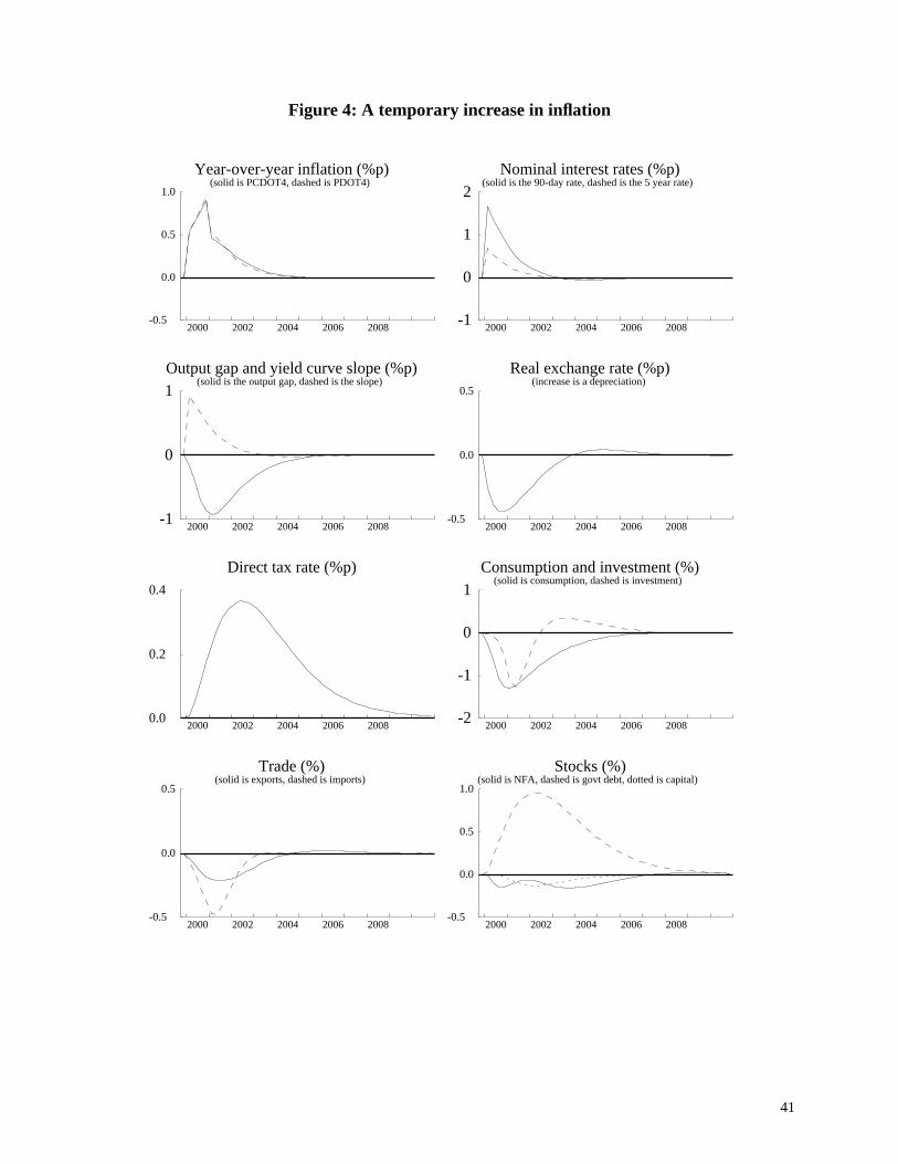
41

Figure 4: A temporary increase in inflation

2000 2002 2004 2006 2008-0.5

0.0

0.5

1.0

Year-over-year inflation (%p)(solid is PCDOT4, dashed is PDOT4)

2000 2002 2004 2006 2008-1

0

1

2Nominal interest rates (%p)

(solid is the 90-day rate, dashed is the 5 year rate)

2000 2002 2004 2006 2008-1

0

1Output gap and yield curve slope (%p)

(solid is the output gap, dashed is the slope)

2000 2002 2004 2006 2008-0.5

0.0

0.5

Real exchange rate (%p)(increase is a depreciation)

2000 2002 2004 2006 20080.0

0.2

0.4

Direct tax rate (%p)

2000 2002 2004 2006 2008-2

-1

0

1Consumption and investment (%)

(solid is consumption, dashed is investment)

2000 2002 2004 2006 2008-0.5

0.0

0.5

Trade (%)(solid is exports, dashed is imports)

2000 2002 2004 2006 2008-0.5

0.0

0.5

1.0

Stocks (%)(solid is NFA, dashed is govt debt, dotted is capital)

42

3.5 An increase in world commodity prices

In this shock, the price of world commodities rises. In CPAM, this shock is introduced as a

10 percentage point increase in the relative price of Canadian exports in world markets.

As CPAM is a model of a small open economy, exporters are price takers. This means that

when prices increase, exporters increase their production, and aggregate exports increase. In

addition, as the shock represents an increase in wealth for consumers, this increase is echoed in the

consumption sector. Overall, aggregate demand increases, and this kicks off an inflation and

monetary policy response that is familiar from the demand shock in Section 3.1. There is also an

apparent difference between thePC and PDFC inflation measures stemming from the exchange

rate appreciation, just as in Section 3.2.

Note the initial decline in aggregate investment. It might be reasonable to expect an increase

here to reflect exporters building up their capital stock. That investment actually falls is due to the

relative price effect, from the appreciation in the dollar, and the impact of the rise in interest rates,

which outweigh the (small) direct effect. This is consistent with the results reported by Macklem

(1993) from a more complete (multi-sector) model. An important point here is that firms know that

this particular shock is temporary. Although we do not show this here, we can report that if the

shock were permanent, there would be a strong increase in investment due to the larger direct effect.

The changes in the real exchange rate here have both a real and a policy (interest rate)

component. The effect of the interest rate is as described above, and operates through the uncovered

interest parity condition (equation 100). The real component comes from the role of the real

exchange rate in supporting the overall asset equilibrium (see Section 2.11). For a given level of

net foreign debt, higher export prices mean that less real output is needed to service that debt. The

pressure is thus for the exchange rate to appreciate to remove some of the shock. One can also think

of this as part of the mechanism whereby the favourable terms-of-trade shock gets passed on to

households. The real appreciation makes imports cheaper and facilitates the brief surge in

consumption.

43

Figure 5: An increase in commodity prices(% is per cent shock minus control, %p is percentage points shock minus control)

2000 2002 2004 2006 2008-0.1

0.0

0.1

0.2

Year-over-year inflation (%p)(solid is PCDOT4, dashed is PDOT4)

2000 2002 2004 2006 2008-0.2

0.0

0.2

0.4

Nominal interest rates (%p)(solid is the 90-day rate, dashed is the 5 year rate)

2000 2002 2004 2006 2008-0.2

0.0

0.2

0.4

Output gap and yield curve slope (%p)(solid is the output gap, dashed is the slope)

2000 2002 2004 2006 2008-0.4

-0.2

0.0

0.2

Real exchange rate (%p)(increase is a depreciation)

2000 2002 2004 2006 2008-0.05

0.00

0.05

Direct tax rate (%p)

2000 2002 2004 2006 2008-0.5

0.0

0.5

Consumption and investment (%)(solid is consumption, dashed is investment)

2000 2002 2004 2006 2008-0.5

0.0

0.5

Trade (%)(solid is exports, dashed is imports)

2000 2002 2004 2006 2008-1

0

1

2Stocks (%)

(solid is NFA, dashed is govt debt, dotted is capital)

44

3.6 An increase in total factor productivity

So much for temporary shocks; we now turn to permanent shocks. In this shock, the level

of total factor productivity increases permanently by 1 per cent.

Such a change has a permanent effect on the steady state of CPAM—all real levels increase

by just over 1.5 per cent (the equivalent increase in labour productivity). However, no ratio of prices

or real variable changes.24 The only exception is relative factor prices; the real wage, however

measured, rises to reflect the higher productivity.

The adjustment to the new steady state commences with an investment boom, as firms put

new capital in place to take advantage of the higher level of productivity. Households also increase

their consumption, in response to their new-found wealth. Both these effects contribute to a large

increase in imports. Exports, too, increase to their new equilibrium level. Overall, the increase in

imports outstrips that of exports, as it must in order thatNFA fall to its new equilibrium level.25

As, initially, supply outstrips demand, the shock is deflationary. In addition, as nominal

wages are sticky, firms pay workers less than their marginal product in the short run. Competition

among firms then leads to a reduction in the inflation rate as firms reduce their (increases in) prices

in line with their lower marginal cost.

Overall,PC inflation falls by a little under 1 percentage point, and the monetary authority

loosens monetary conditions accordingly.

24. This is different from QPM where the economy is not, strictly speaking, a small open economy so theincrease in domestic productivity leads to a modest depreciation in the exchange rate. This, in turn, affectsthe cost of capital and the rest of the model.

25. As Canada is a net debtor,NFA is negative. In order that theNFA-to-GDP ratio be constant, this means thatNFA must decrease (i.e., become more negative).

45

Figure 6: An increase in total factor productivity(% is per cent shock minus control, %p is percentage points shock minus control)

2000 2002 2004 2006 2008-2

-1

0

1Year-over-year inflation (%p)

(solid is PCDOT4, dashed is PDOT4)

2000 2002 2004 2006 2008-2

-1

0

1Nominal interest rates (%p)

(solid is the 90-day rate, dashed is the 5 year rate)

2000 2002 2004 2006 2008-2

-1

0

1Output gap and yield curve slope (%p)

(solid is the output gap, dashed is the slope)

2000 2002 2004 2006 20080.0

0.2

0.4

Real exchange rate (%p)(increase is a depreciation)

2000 2002 2004 2006 2008-1.0

-0.5

0.0

0.5

Direct tax rate (%p)

2000 2002 2004 2006 20080

5

10Consumption and investment (%)

(solid is consumption, dashed is investment)

2000 2002 2004 2006 20080

1

2

3Trade (%)

(solid is exports, dashed is imports)

2000 2002 2004 2006 2008-2

0

2Stocks (%)

(solid is NFA, dashed is govt debt, dotted is capital)

46

3.7 A change in the target rate of inflation

The last two shocks illustrate how CPAM is useful for analyzing changes in policy. In this

subsection, the monetary authority reduces its target inflation rate by 1 percentage point.

In CPAM, there are no free lunches in the form of announcement effects, so the monetary

authority must tighten monetary conditions in order to reduce the inflation rate to its new level. It

does so, and the slope of the yield curve increases by 1 percentage point in the first year. This

triggers an appreciation of the currency, which helps move consumption prices down, initially, and

also adds to the reduction of aggregate demand through the trade balance. A negative output gap

emerges, and the inflation rate declines until it reaches its new target level.

This shock also illustrates some aspects of interest rate determination in CPAM. In CPAM,

the long-term rate is based on the expectations hypothesis, but with a little extra weight on current

conditions, such that the long rate tends to move more with the short rate than would be predicted

by the expectations hypothesis. Nevertheless, as the monetary authority has credibility, in the sense

that agents know that it will carry out the planned reduction in the rate of inflation, the long-term

interest rate falls immediately.26 This means that the short rate does not have to be raised as much

as the slope to achieve the objective. In this respect, it is interesting to contrast this shock with the

temporary shock to inflation in Section 3.4. There, in contrast, the long rate rises with the short rate,

and so the short rate has to rise relatively more to reverse inflation than it does here to reduce it.

One common measure of the costs of disinflation, is the sacrifice ratio, measured as the

cumulative loss in output necessary to reduce inflation permanently by 1 percentage point. CPAM

has been calibrated to have a sacrifice ratio of just under 2.7, which is slightly less than in QPM.

26. In QPM, the long rate increases slightly for the first few quarters of the shock.

47

Figure 7: An decrease in the target rate of inflation(% is per cent shock minus control, %p is percentage points shock minus control)

2000 2002 2004 2006 2008-2

-1

0

1Year-over-year inflation (%p)

(solid is PCDOT4, dashed is PDOT4)

2000 2002 2004 2006 2008-2

-1

0

1Nominal interest rates (%p)

(solid is the 90-day rate, dashed is the 5 year rate)

2000 2002 2004 2006 2008-2

0

2Output gap and yield curve slope (%p)

(solid is the output gap, dashed is the slope)

2000 2002 2004 2006 2008-1.0

-0.5

0.0

0.5

Real exchange rate (%p)(increase is a depreciation)

2000 2002 2004 2006 20080.0

0.2

0.4

Direct tax rate (%p)

2000 2002 2004 2006 2008-2

-1

0

1Consumption and investment (%)

(solid is consumption, dashed is investment)

2000 2002 2004 2006 2008-1.0

-0.5

0.0

0.5

Trade (%)(solid is exports, dashed is imports)

2000 2002 2004 2006 2008-0.5

0.0

0.5

1.0

Stocks (%)(solid is NFA, dashed is govt debt, dotted is capital)

48

3.8 A permanent change in government debt

In this shock, the government lowers the target ratio of debt to GDP by 10 percentage

points. To analyse this shock, it is convenient to start with the steady-state implications, and then

move to the dynamic effects.

The basic result from the steady-state model is that, as the direct tax rate is lower in the end,

consumers have more wealth, and this leads to an increase in consumption of 0.46 per cent. The

lower tax rate reflects the lower debt-service burden in the new steady state. There is also a

substantial reallocation of assets within the portfolio, as consumers switch from holding

government assets to holding net foreign assets. The ratio of net foreign assets to GDP increases by

just over 10 percentage points. Finally, a small relative price effect reduces the cost of capital and

output increases by 0.03 per cent.27

Moving now to the dynamics, we see that a key difference arises from the profile of the

personal tax rate. Though it will eventually fall below control, it has to rise sharply at first to secure

the revenues to pay off part of the debt. Hence, although consumption is higher in the steady state,

the increased tax burden during the adjustment means that consumption over the medium term is

depressed. Indeed, consumption falls by over 6 per cent, relative to control, in the first couple of

years of the shock, and does not rise above control until year five. Such a large reduction in

consumption leads to a significant decline in imports, and it is this, supported by a depreciation in

the currency and the consequential increase in exports, that facilitates the substitution away from

government debt towards net foreign assets.

The short-term implications of the shock for the monetary authority are interesting. Overall,

the economy is in a position of excess supply, so PDFC inflation falls. However, the strong

depreciation of the currency causes the inflation rate, as measured by consumer prices, to increase

slightly in the first year before the effects of depressed demand pull it down too. As the monetary

authority looks past the initial rise in consumer price inflation to the period where it will be below

control, they loosen monetary conditions from the start. With a less forward-looking policy rule,

there would be less willingness to ease early and to let the exchange rate depreciate as part of the

adjustment.

27. The reader is referred to Black, Laxton, Rose, and Tetlow (1994) for a more detailed discussion of the steady-state implications of this shock.

49

Figure 8: An decrease in the target debt-to-GDP ratio(% is per cent shock minus control, %p is percentage points shock minus control)

2000 2002 2004 2006 2008-0.5

0.0

0.5

Year-over-year inflation (%p)(solid is PCDOT4, dashed is PDOT4)

2000 2002 2004 2006 2008-2

-1

0

1Nominal interest rates (%p)

(solid is the 90-day rate, dashed is the 5 year rate)

2000 2002 2004 2006 2008-4

-2

0

2Output gap and yield curve slope (%p)

(solid is the output gap, dashed is the slope)

2000 2002 2004 2006 2008-2

0

2

4Real exchange rate (%p)

(increase is a depreciation)

2000 2002 2004 2006 2008-5

0

5

10Direct tax rate (%p)

2000 2002 2004 2006 2008-10

-5

0

5

Consumption and investment (%)(solid is consumption, dashed is investment)

2000 2002 2004 2006 2008-5

0

5Trade (%)

(solid is exports, dashed is imports)

2000 2002 2004 2006 2008-50

0

50

Stocks (%)(solid is NFA, dashed is govt debt, dotted is capital)

50

APPENDIX A: The adjustment mechanism in CPAM

This appendix describes the generic adjustment process used in CPAM. CPAM has

dynamics arising from three main sources. The first is intrinsic dynamics, that is, dynamic structure

that arises from the tendency for economic agents to adjust gradually to disturbances, even when

those disturbances are understood perfectly. Such behaviour arises when adjustment is costly. The

other two general sources of dynamic structure in CPAM are expectations formation and the

endogenous response of monetary and fiscal policy to economic conditions. The focus of this

appendix is on the first source; the other two have been addressed in the main text.

In CPAM, intrinsic dynamics are modelled as the solution to a quadratic optimization

problem. In this problem, agents must weigh a cost of being away from a target with the cost of

adjusting towards it. The result is that agents adjust “slowly” towards the new target, with “slowly”

being defined as a matter of calibration. The following discussion is based on Pesaran (1991) and

particularly on the formulation in Tinsley (1993).

The generic dynamic adjustment model

Let be the variable to be modelled, and its “desired” value in the absence of adjustment

costs. At time , the general intrinsic adjustment model is derived from choosing , for ,

to minimize the following cost function:

(A1) ,

where is a polynomial in the lag operator and is the order of the adjustment process. The

first term of this equation penalizes being away the desired level. The second term, which is made

up of quadratic terms of past values of , is chosen so as to penalize changes in . Note that,

given the definitions of below, having high weights will penalize changes in and lead to

gradual adjustment.

y y*

t yt τ+ τ 0≥

E yt τ+ yt τ+*–( )2 0.5 φi Ai L( )yt τ+( )2

i 0=

n

∑+τ 0=

∞

∑

Ai L( ) n

n y y

Ai φ y

51

In CPAM, two different forms for are used, depending on whether the adjustment is for

a stock or not. If the adjustment is for a flow or a relative price, then is chosen so that changes

in the (equally-weighted) moving average of are penalized. This change is given by

(A2) ,

so that is given by

(A3) .

For stocks, in particular capital, is chosen so that changes in the difference of are

penalized. This leads to the definition

(A4) .

Having these two different styles of adjustment costs facilitates the calibration of the model.

For flows, the data suggest that past flows are good indicators of the current flow. This is captured

in the model by placing high weights on changes in moving averages. As can be seen in equation

(2), this penalizes a movement in compared to what it was in the past. For stocks, the problem is

slightly different. In this case, it was found that, when the first form of adjustment is used, even

though the dynamics of stock itself look fine, the flows resulting from the changes in the stock are

very volatile. The second form, which penalizes differences, provides a similar path for the level of

the stock, but one with smoother changes in flows.

The solution to minimization of (1) is a straightforward application of dynamic

programming, and results in an Euler equation in lags and leads.28 In CPAM, the equations

are left in this form, unlike in QPM where they are rewritten as an infinite sum and truncated. The

leads are taken to be model-consistent expectations. The solution can be written in the form:

(A5) ,

as in the main text, where is a function that depends on leads and lags of as well as

the parameters in and .

28. In CPAM, these Euler equations are generated using a TROLL macro.

Ai

Ai

i th y

yt τ j–+( )j 0=

i

∑ yt τ 1– j–+( )j 0=

i

∑– yt τ+ yt τ 1–+–=

Ai

Ai L( ) 1 Li 1+

+=

Ai i th y

Ai L( ) 1 L–( )i=

φ

y

n n

y y* yadj–=

yadj n 1– y

A φ

52

An example of a customized equation

Take the case of the model's equation for the dynamics of consumer spending (by forward-

looking consumers). This is given by a fourth-order adjustment model that penalizes changes in

moving averages. The target rate is given by

(A6) .

In addition to the equilibrium value of consumption, there are several other terms in this equation.

The first two, with coefficients and , are there to capture special features of cyclical

correlation among economic variables. These have been described in the main text. There is also a

third extra term, , that can be used to shock consumption.

The solution to this, as noted in (5), can be written as

(A7) .

For completeness, the term is included below. For this equation, we return to TROLL

syntax; it is the equation exactly as generated by the TROLL macro described earlier.

(A8)CFLADJ CFLADJ = CD1*(1*1*1*(1*1* CFL(0)-1*1*CFL(-1))

-1*1*CB1**1*(1*1* CFL(1)-1*1*CFL(0)))+CD2*(1*1*1*(1*1* CFL(0)

-1*2*CFL(-1)+1*1*CFL(-2))-1*2*CB1**1*(1*1* CFL(1)

-1*2*CFL(0)+1*1*CFL(-1))+1*1*CB1**2*(1*1* CFL(2)

-1*2*CFL(1)+1*1*CFL(0)))+CD3*(1*1*1*(1*1* CFL(0)

-1*3*CFL(-1)+1*3*CFL(-2)-1*1*CFL(-3))-1*3*CB1**1*(1*1* CFL(1)

-1*3*CFL(0)+1*3*CFL(-1)-1*1*CFL(-2))+1*3*CB1**2*(1*1* CFL(2)

-1*3*CFL(1)+1*3*CFL(0)-1*1*CFL(-1))-1*1*CB1**3*(1*1* CFL(3)

-1*3*CFL(2)+1*3*CFL(1)-1*1*CFL(0)))+CD4*(1*1*1*(1*1* CFL(0)-

1*4*CFL(-1)+1*6*CFL(-2)-1*4*CFL(-3)+1*1*CFL(-4))

-1*4*CB1**1*(1*1* CFL(1)-1*4*CFL(0)+1*6*CFL(-1)

-1*4*CFL(-2)+1*1*CFL(-3))+1*6*CB1**2*(1*1* CFL(2)

-1*4*CFL(1)+1*6*CFL(0)-1*4*CFL(-1)+1*1*CFL(-2))

-1*4*CB1**3*(1*1* CFL(3)-1*4*CFL(2)+1*6*CFL(1)-1*4*CFL(0)

+1*1*CFL(-1))+1*1*CB1**4*(1*1* CFL(4)-1*4*CFL(3)+1*6*CFL(2)

-1*4*CFL(1)+1*1*CFL(0)))

cfl* cfleq λ1 r r

eq–( ) λ2 nfa nfaeq–( )+– cflshk+=

λ1 λ2

cflshk

cfl cfleq λ1 r r

eq–( ) λ2 nfa nfaeq–( )+– cflshk cfladj–+=

cfladj

53

APPENDIX B:Mnemonics, descriptions, and values

This appendix contains the mnemonics and descriptions of the variables and parameters in

the model CPAM. They are grouped by endogenous, exogenous, and parameter types. Variables

that are exogenous for calibration only are labelled as such with an indication to the corresponding

variable that is made endogenous. The values shown for exogenous and endogenous variables are

their steady-state values.

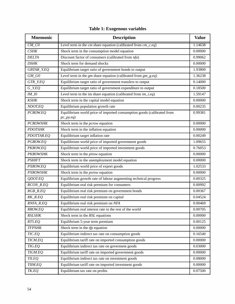
54

Table 1: Exogenous variables

Mnemonic Description Value

CM_C0 Level term in thecm share equation (calibrated fromcm_c.eq) 1.14638

CSHK Shock term in the consumption model equation 0.00000

DELTA Discount factor of consumers (calibrated fromnfa) 0.99062

DSHK Shock term for demand shocks 0.00000

GBTAR_Y.EQ Equilibrium target ratio of government bonds to output 1.93800

GM_G0 Level term in thegm share equation (calibrated fromgm_g.eq) 1.36238

GTR_Y.EQ Equilibrium target ratio of government transfers to output 0.14000

G_Y.EQ Equilibrium target ratio of government expenditure to output 0.18500

IM_I0 Level term in the im share equation (calibrated from im_i.eq) 1.59147

KSHK Shock term in the capital model equation 0.00000

NDOT.EQ Equilibrium population growth rate 0.00235

PCROW.EQ Equilibrium world price of imported consumption goods (calibrated frompc_py.eq)

0.99381

PCROWSHK Shock term in thepcrow equation 0.00000

PDOTSHK Shock term in the inflation equation 0.00000

PDOTTAR.EQ Equilibrium target inflation rate 0.00249

PGROW.EQ Equilibrium world price of imported government goods 1.09655

PKROW.EQ Equilibrium world price of imported investment goods 0.76053

PKROWSHK Shock term in thepirow equation 0.00000

PSHIFT Shock term in the unemployment model equation 0.00000

PXROW.EQ Equilibrium world price of export goods 1.02533

PXROWSHK Shock term in thepxrow equation 0.00000

QDOT.EQ Equilibrium growth rate of labour augmenting technical progress 0.00325

RCON_R.EQ Equilibrium real risk premium for consumers 0.00992

RGB_R.EQ Equilibrium real risk premium on government bonds 0.00367

RK_R.EQ Equilibrium real risk premium on capital 0.04524

RNFA_R.EQ Equilibrium real risk premium onNFA 0.00469

RROW.EQ Equilibrium real interest rate in the rest of the world 0.00705

RSLSHK Shock term in the RSL equations 0.00000

RT5.EQ Equilibrium 5-year term premium 0.00125

TFPSHK Shock term in thetfp equation 0.00000

TIC.EQ Equilibrium indirect tax rate on consumption goods 0.16540

TICM.EQ Equilibrium tariff rate on imported consumption goods 0.00000

TIG.EQ Equilibrium indirect tax rate on goverment goods 0.03000

TIGM.EQ Equilibrium tariff rate on imported government goods 0.00000

TII.EQ Equilibrium indirect tax rate on investment goods 0.08000

TIIM.EQ Equilibrium tariff rate on imported investment goods 0.00000

TK.EQ Equilibrium tax rate on profits 0.07500

55

TUNE_RSL Utility variable for delaying monetary policy response 1.00000

TUNE_Z Utility variable for holding the exchange rate fixed, temporarily 1.00000

U.EQ Equilibrium rate of unemployment 0.08000

USHK Shock term in the unemployment model equation 0.00000

WSHK Shock term in the real wage equation 0.00000

XM_X.EQ Equilibrium ratio of imports for re-export (calibrated from x.eq) 0.34921

X_Y0 Level term in the equilibrium export equation (calibrated fromz) -0.59507

ZSHK Shock term in the real exchange rate equation 0.00000

Table 1: Exogenous variables

Mnemonic Description Value

56

Table 2: Endogenous variables

Mnemonic Description Value

C Consumption 0.17300

C.EQ Equilibrium consumption 0.17300

CC.EQ Equilibrium user cost of capital 0.06367

CFL Consumption by forward-looking consumers 0.12209

CFL.EQ Equilibrium consumption by forward-looking consumers 0.12209

CFLADJ cfladjustment cost 0.00000

CHECK1.EQ A check on the equilibrium SNA identity 0.00000

CHECK2.EQ A check on the equilibriumPD identity 0.00000

CM Imports of consumption goods 0.03308

CM.EQ Equilibrium imports of consumption goods 0.03308

CM_C Share of imported consumption goods 0.19120

CM_C.EQ Equilibrium share of imported consumption goods (calibratescm_c0) 0.19120

CM_CADJ cm_c adjustment cost 0.00000

CRT Consumption by rule-of-thumb consumers 0.05091

CRT.EQ Equilibrium consumption by rule-of-thumb consumers 0.05091

D Demand index (c+i) 0.20984

FA Real financial assets 1.27983

FA.EQ Equilibrium financial assets 1.27983

FA.SS Steady-state financial assets 1.27983

G Real government expenditures 0.04625

G.EQ Equilibrium government expenditures 0.04625

GB Real government assets 0.48450

GB.EQ Equilibrium government assets 0.48450

GBTAR Government target debt level 0.48450

GM Imports of government goods 0.01641

GM.EQ Equilibrium imports of government goods 0.01641

GM_G Share of imported government goods 0.35490

GM_G.EQ Equilibrium share of imported government goods (calibratesgm_g0) 0.35490

GM_GADJ gm_g adjustment cost 0.00000

GTR Real government transfers 0.03500

GTR.EQ Equilibrium government transfers 0.03500

HWFL.EQ Equilibrium human wealth 5.19519

I Real investment 0.03684

I.EQ Equilibrium investment 0.03684

I.SS Steady-state investment 0.03684

IM Imports of investment goods 0.02225

IM.EQ Equilibrium imports of investment goods 0.02225

IM_I Share of imported investment goods 0.60390

57

IM_I.EQ Equilibrium share of imported investment goods (calibrates im_i0) 0.60390

IM_IADJ im_i adjustment cost -0.00000

K Production capital 1.37645

K.EQ Equilibrium production capital 1.37645

KADJ k adjustment cost 0.00000

M Imports 0.10697

M.EQ Equilibrium imports 0.10697

MPCW.EQ Equilibrium marginal propensity to consume out of wealth 0.02202

NDOT Population growth rate 0.00235

NETX Real net exports 0.00229

NETX.EQ Equilibrium net exports 0.00229

NFA Net foreign asset ratio -0.31122

NFA.EQ Equilibrium net foreign asset ratio (calibratesdelta) -0.31122

PC Relative price of consumption goods 1.17076

PC.EQ Equilibrium relative price of consumption goods 1.17076

PCD Relative price of domestic consumption goods 1.01328

PCD.EQ Equilibrium relative price of domestic consumption goods 1.01328

PCDADJ pcd adjustment cost 0.00000

PCDOT Inflation rate for PC 0.00249

PCDOT4 4-quarter inflation rate forPC 0.00249

PCDOTE Expected PC inflation rate 0.00249

PCDOTEA Effective average expectedPC inflation rate 0.00249

PCLEVEL Level price of consumption goods 1.69447

PCLEVELTAR Optional term for price-level targeting 1.69447

PCM Relative price of imported consumption goods 0.96787

PCM.EQ Equilibrium relative price of imported consumption goods 0.96787

PCMADJ pcm adjustment cost 0.00000

PCROW World price of imported consumption goods 0.99381

PC_PY.EQ Equilibrium price of consumption relative topy 1.02670

PDOT Inflation rate for PDFC 0.00249

PDOT.EQ Equilibrium inflation rate 0.00249

PDOT4 4-quarter inflation rate forP 0.00249

PDOTE Expected inflation rate 0.00249

PDOTEA Effective average expectedP inflation rate 0.00249

PDOTTAR Target inflation rate 0.00249

PDOTTARE Expected target inflation rate 0.00249

PFC Relative price of output at factor cost 1.01065

PFC.EQ Equilibrium relative price of output at factor cost 1.01065

Table 2: Endogenous variables

Mnemonic Description Value

58

PG Relative price of government goods 1.09470

PG.EQ Equilibrium relative price of government goods 1.09470

PGD Equilibrium relative price of domestic government goods 1.06000

PGD.EQ Equilibrium relative price of domestic government goods (cals. frompg_py.eq) 1.06000

PGDADJ pgd adjustment cost 0.00000

PGM Relative price of imported government goods 1.06793

PGM.EQ Equilibrium relative price of imported government goods 1.06793

PGMADJ pgm adjustment cost 0.00000

PGROW World price of imported government goods 1.09655

PG_PY.EQ Equilibrium price of government goods relative topy (calibratespg.eq) 0.96000

PI.EQ Equilibrium relative price of capital goods 0.80392

PK Relative price of investment goods 0.80392

PK.EQ Equilibrium relative price of investment goods 0.80392

PK.SS Steady-state relative price of investment goods 0.80392

PKD Relative price of domestic investment goods 0.75000

PKD.EQ Equilibrium relative price of domestic investment goods 0.75000

PKDADJ pkd adjustment cost 0.00000

PKM Relative price of imported investment goods 0.74068

PKM.EQ Equilibrium relative price of imported investment goods 0.74068

PKMADJ pkm adjustment cost 0.00000

PKROW World price of imported investment goods 0.76053

PK_PY.EQ Equilibrium price of investment relative to py 0.70500

PM Relative price of import goods 0.92030

PM.EQ Equilibrium relative price of import goods 0.92030

PM_PY.EQ Equilibrium price of import goods relative topy 0.80707

PX Relative price of export goods 0.99857

PX.EQ Equilibrium relative price of export goods 0.99857

PXADJ px adjustment cost 0.00000

PXM Relative price of imported export goods 0.92030

PXM.EQ Equilibrium relative price of imported export goods 0.92030

PXROW World price of export goods 1.02533

PX_PY.EQ Equilibrium price of export goods relative topy (calibratespxrow.eq) 0.87570

PY Relative price of output 1.14031

PY.EQ Equilibrium relative price of output at market prices 1.14031

PYDOT Inflation rate forPY 0.00249

QDOT Trend growth in labour augmenting technical progress 0.00325

R Real interest rate 0.00705

R.EQ Equilibrium real interest rate 0.00705

Table 2: Endogenous variables

Mnemonic Description Value

59

R5 5-year moving average of real rates 0.00831

R5.EQ Equilibrium 5-year moving average of real rates 0.00831

RCON.EQ Equilibrium real interest rate for consumers 0.01823

RGB Real interest rate for government assets 0.01198

RGB.EQ Equilibrium real return on government bonds 0.01198

RISK Transfer to individuals from asset holders 0.03747

RISK.EQ Equilibrium transfer to individuals from asset holders 0.03747

RK.EQ Equilibrium real interest rate for capital 0.05354

RL Real long interest rate 0.00831

RL.EQ Equilibrium real long interest rate 0.00831

RN Nominal interest rate 0.00956

RN.EQ Equilibrium nominal interest rate 0.00956

RN5 5-year moving average of nominal rates 0.01082

RN5.EQ Equilibrium 5-year moving average of nominal rates 0.01082

RNFA Real interest rate for net foreign assets 0.01300

RNFA.EQ Equilibrium real return on net foreign assets 0.01300

RNL Nominal long interest rate 0.01082

RNL.EQ Equilibrium nominal long interest rate 0.01082

RROW Real interest rate in the rest of the world 0.00705

RSL Slope of the yield curve -0.00125

RSL.EQ Equilibrium slope of the yield curve -0.00125

TD Net direct tax rate 0.28144

TD.EQ Equilibrium net direct tax rate 0.28144

TFP Total factor productivity 0.94777

TFP.EQ Equilibrium level of total factor productivity (calibrated fromy) 0.94777

TIC Indirect tax rate on consumption goods 0.16540

TICM Tariff rate on imported consumption goods 0.00000

TIG Indirect tax rate on government goods 0.03000

TIGM Tariff rate on imported government goods 0.00000

TII Indirect tax rate on investment goods 0.08000

TIIM Tariff rate on imported investment goods 0.00000

TK Tax rate on profits 0.07500

TWFL.EQ Equilibrium total wealth 6.49109

U Rate of unemployment 0.08000

UADJ uadjustment cost 0.00000

W Relative wage 0.17991

W.EQ Equilibrium relative wage 0.17991

WADJ w adjustment cost -0.00000

Table 2: Endogenous variables

Mnemonic Description Value

60

WC Consumer real wage 0.15367

WC.EQ Equilibrium consumer real wage 0.15367

WP Producer real wage 0.17802

WP.EQ Equilibrium producer real wage 0.17802

X Exports 0.10088

X.EQ Equilibrium exports 0.10088

XADJ x adjustment cost 0.00000

XM Imports for re-export 0.03523

XM.EQ Equilibrium imports for re-export 0.03523

XM_X Share of imports for re-export 0.34921

Y Output 0.25000

Y.EQ Equilibrium output (calibrates tfp.eq) 0.25000

YDFL Real disposable income for forward-looking consumers 0.08941

YDFL.EQ Equilibrium disposable income for forward-looking consumers 0.08941

YDOT Trend output growth rate 0.00561

YDOT.EQ Equilibrium output growth rate 0.00561

YDRT Real disposable income for rule-of-thumb consumers 0.05960

YDRT.EQ Equilibrium disposable income for rule-of-thumb consumers 0.05960

YLAB Real labour income 0.16552

YLAB.EQ Equilibrium real labour income 0.16552

YP Potential output 0.25000

Z Real price of foreign exchange 0.97390

Z.EQ Equilibrium real price of foreign exchange (calibratesX_Y0) 0.97390

Z.SS Steady-state real price of foreign exchange 0.97390

ZE Expected real price of foreign exchange 0.97390

Table 2: Endogenous variables

Mnemonic Description Value

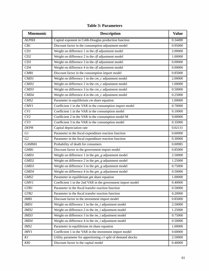
61

Table 3: Parameters

Mnemonic Description Value

ALPHA Capital exponent in Cobb-Douglas production function 0.34490

CB1 Discount factor in the consumption adjustment model 0.95000

CD1 Weight on difference 1 in thecfl adjustment model 2.00000

CD2 Weight on difference 2 in thecfl adjustment model 1.00000

CD3 Weight on difference 3 in thecfl adjustment model 0.00000

CD4 Weight on difference 4 in thecfl adjustment model 0.00000

CMB1 Discount factor in the consumption import model 0.85000

CMD1 Weight on difference 1 in thecm_c adjustment model 2.00000

CMD2 Weight on difference 2 in thecm_c adjustment model 1.00000

CMD3 Weight on difference 3 in thecm_c adjustment model 0.50000

CMD4 Weight on difference 4 in thecm_c adjustment model 0.25000

CMS2 Parameter in equilibriumcm share equation 1.00000

CMV1 Coefficient 1 in the VAR in the consumption import model 0.70000

CV1 Coefficient 1 in the VAR in the consumption model 0.10000

CV2 Coefficient 2 in the VAR in the consumption model M 9.00000

CV3 Coefficient 3 in the VAR in the consumption model 0.35000

DEPR Capital depreciation rate 0.02131

G1 Parameter in the fiscal expenditure reaction function 0.60000

G2 Parameter in the fiscal expenditure reaction function 0.30000

GAMMA Probability of death for consumers 0.00985

GMB1 Discount factor in the government import model 0.85000

GMD1 Weight on difference 1 in thegm_g adjustment model 2.50000

GMD2 Weight on difference 2 in thegm_gadjustment model 1.25000

GMD3 Weight on difference 3 in thegm_g adjustment model 0.75000

GMD4 Weight on difference 4 in thegm_g adjustment model 0.50000

GMS2 Parameter in equilibriumgm share equation 1.00000

GMV1 Coefficient 1 in the 2nd VAR in the government import model 0.40000

GTR1 Parameter in the fiscal transfer reaction function 0.50000

GTR2 Parameter in the fiscal transfer reaction function 0.20000

IMB1 Discount factor in the investment import model 0.85000

IMD1 Weight on difference 1 in theim_i adjustment model 2.50000

IMD2 Weight on difference 2 in theim_i adjustment model 1.25000

IMD3 Weight on difference 3 in theim_i adjustment model 0.75000

IMD4 Weight on difference 4 in theim_i adjustment model 0.50000

IMS2 Parameter in equilibrium im share equation 1.00000

IMV1 Coefficient 1 in the VAR in the investment import model 0.60000

K1 Utility parameter for apportioningc/i split of demand shocks 2.50000

KB1 Discount factor in the capital model 0.40000

62

KD1 Weight on difference 1 in thek adjustment model 6.00000

KD2 Weight on difference 2 in thek adjustment model 4.00000

KD3 Weight on difference 3 in the k adjustment model 3.00000

KD4 Weight on difference 4 in thek adjustment model 1.00000

KE1 Weight onk.eq adjustment term in thecc.eq equation 0.55000

KV1 Coefficient 1 in the VAR in the capital model 0.18000

KV2 Coefficient 2 in the VAR in the capital model 1.10000

LAMDA Proportion of rule-of-thumb consumers in the population 0.40000

PCDB1 Discount factor for thepcd adjustment model 0.95000

PCDD1 Weight on difference 1 in the pcd adjustment model 0.00000

PCDD2 Weight on difference 2 in thepcd adjustment model 0.00000

PCDD3 Weight on difference 3 in thepcd adjustment model 0.00000

PCDD4 Weight on difference 4 in thepcd adjustment model 0.00000

PCM1 Pass-through coefficient, relative imported consumption.eq trade prices 0.80000

PCMB1 Discount factor in the price of consumption imports model 0.95000

PCMD1 Weight on difference 1 in the pcm adjustment model 2.00000

PCMD2 Weight on difference 2 in thepcm adjustment model 1.00000

PCMD3 Weight on difference 3 in thepcm adjustment model 0.00000

PCMD4 Weight on difference 4 in thepcm adjustment model 0.00000

PCMV1 Pass-through coefficient, relative imported consumption trade prices 0.50000

PCMV2 Coefficient 2 in the VAR in thepcm model 0.80000

PD0 Coefficient on the gap in the inflation equation 0.02000

PD1 Coefficient on lagged gap in the inflation equation 0.04000

PD2 Coefficient on the positive gap in the inflation equation 0.09000

PD3 Coefficient on the lagged positive gap in the inflation equation 0.03000

PD4 Coefficient on wage effects in the inflation equation 2.00000

PD5 Coefficient on wages changes in the inflation equation 0.60000

PD6 Coefficient on wages changes in the inflation equation 0.25000

PD7 Coefficient on wages changes in the inflation equation 0.15000

PDA1 Weight on lagged inflation in the inflation equation 0.35000

PDA2 Weight on second lag of inflation in the inflation equation 0.25000

PDA3 Weight on third lag of inflation in the inflation equation 0.20000

PDA4 Relative weight of producer price expectations 0.60000

PDA5 Coefficient on import price change in the inflation equation 0.05000

PDA6 Coefficient on export price change in the inflation equation 0.05000

PDE0 Weight on the expected target in P inflation expectations 0.10000

PDE1 Weight on the lead inP inflation expectations 0.55000

PDE2 Weight on the lead inPC inflation expectations 0.55000

Table 3: Parameters

Mnemonic Description Value

63

PDE3 Weight on the expected target inPC inflation expectations 0.10000

PDE4 Weight on the level gap in inflation expectations 0.00000

PDF1 Weight on trend expectations in the inflation equation 0.25000

PDF2 Weight on expected inflation in the inflation equation 0.43000

PDL1 Weight on laggedpdot in the inflation expectations equation 0.70000

PGDB1 Discount factor in thepgd model 0.95000

PGDD1 Weight on difference 1 in thepgd adjustment model 1.00000

PGDD2 Weight on difference 2 in thepgd adjustment model 0.00000

PGDD3 Weight on difference 3 in thepgd adjustment model 0.00000

PGDD4 Weight on difference 4 in thepgd adjustment model 0.00000

PGDV1 Coefficient 1 in the VAR in thepgd model 0.05000

PGM1 Pass-through coefficient, relative imported government.eq trade prices 0.80000

PGMB1 Discount factor in the price of government imports model 0.95000

PGMD1 Weight on difference 1 in thepgm adjustment model 2.00000

PGMD2 Weight on difference 2 in thepgm adjustment model 1.00000

PGMD3 Weight on difference 3 in thepgm adjustment model 0.00000

PGMD4 Weight on difference 4 in thepgm adjustment model 0.00000

PGMV1 Pass-through coefficient, relative import government trade prices 0.50000

PGMV2 Coefficient 2 in the VAR in the price of government imports model 0.80000

PK1 Parameter in definition of price of capital goods 0.45000

PKDB1 Discount factor in thepkd model 0.95000

PKDD1 Weight on difference 1 in thepkd adjustment model 1.00000

PKDD2 Weight on difference 2 in thepkd adjustment model 0.00000

PKDD3 Weight on difference 3 in thepkd adjustment model 0.00000

PKDD4 Weight on difference 4 in thepkd adjustment model 0.00000

PKDV1 Coefficient 1 in the VAR in thepkd model 0.00000

PKM1 Pass-through coefficient, relative imported investment.eq trade prices 0.80000

PKMB1 Discount factor in the price of investment imports model 0.95000

PKMD1 Weight on difference 1 in thepkm adjustment model 2.00000

PKMD2 Weight on difference 2 in thepkm adjustment model 1.00000

PKMD3 Weight on difference 3 in thepkm adjustment model 0.00000

PKMD4 Weight on difference 4 in thepkm adjustment model 0.00000

PKMV1 Pass-through coefficient, relative imported investment trade prices 0.50000

PKMV2 Coefficient 2 in the VAR in thepkm model 0.80000

PTL1 Weight on laggedpdottar in thepdottar expectations equation 1.35000

PTL2 Weight on 2nd laggedpdottar in thepdottar expectations equation -0.42500

PTL3 Weight on forwardpdot in thepdottar expectations equation 1.00000

PX1 Pass-through coefficient, relative export .eq trade prices 0.75000

Table 3: Parameters

Mnemonic Description Value

64

PXB1 Discount factor in the price of exports model 0.95000

PXD1 Weight on difference 1 in thepx adjustment model 0.80000

PXD2 Weight on difference 2 in thepx adjustment model 0.50000

PXD3 Weight on difference 3 in thepxadjustment model 0.00000

PXD4 Weight on difference 4 in thepxadjustment model 0.00000

PXV1 Pass-through coefficient, relative export trade prices 0.50000

PXV2 Coefficient 2 in the VAR for the price of exports 0.00000

PXV3 Coefficient 3 in the VAR for the price of exports 0.10000

RI1 Parameter in the risk equation 0.95000

RL1 Weight on the short rate in therl equation 0.30000

RL2 Weight on ther5 rate in therl equation 0.50000

RSL0 Coefficient on inflation gap, lead 0, monetary reaction function 0.00000

RSL1 Coefficient on inflation gap, lead 1, monetary reaction function 0.00000

RSL2 Coefficient on inflation gap, lead 2, monetary reaction function 0.00000

RSL3 Coefficient on inflation gap, lead 3, monetary reaction function 0.00000

RSL4 Coefficient on inflation gap, lead 4, monetary reaction function 0.00000

RSL5 Coefficient on inflation gap, lead 5, monetary reaction function 0.00000

RSL6 Coefficient on inflation gap, lead 6, monetary reaction function 0.00000

RSL7 Coefficient on inflation gap, lead 7, monetary reaction function 1.57500

RSL8 Coefficient on inflation gap, lead 8, monetary reaction function 1.80000

RSL9 Coefficient on inflation gap, lead 9, monetary reaction function 0.00000

RSL10 Coefficient on inflation gap, lead 10, monetary reaction function 0.00000

RSL11 Coefficient on inflation gap, lead 11, monetary reaction function 0.00000

RSL12 Coefficient on inflation gap, lead 12, monetary reaction function 0.00000

RSL13 Coefficient on price level gap, monetary reaction function 0.00000

SIGMA Coefficient of intertemporal substitution for forward-looking consumers 0.66000

TD0 Parameter in the fiscal tax reaction function 0.40000

TD1 Parameter in the fiscal tax reaction function 0.250000

TD3 Parameter in the fiscal tax reaction function 0.80000

UB1 Discount factor in the unemployment model 0.95000

UD1 Weight on difference 1 in the u adjustment model 1.00000

UD2 Weight on difference 2 in theu adjustment model 0.50000

UD3 Weight on difference 3 in theu adjustment model 0.00000

UD4 Weight on difference 4 in theu adjustment model 0.00000

UV1 Coefficient on the wage gap in the unemployment equation 0.06700

UV2 Coefficient onygap(-2) in the unemployment equation 0.22500

UV3 Coefficient onygap(-3) in the unemployment equation 0.22500

WB1 Discount factor in the real wage model 0.95000

Table 3: Parameters

Mnemonic Description Value

65

WD1 Weight on difference 1 in thew adjustment model 1.50000

WD2 Weight on difference 2 in thew adjustment model 1.00000

WD3 Weight on difference 3 in thew adjustment model 0.75000

WD4 Weight on difference 4 in thew adjustment model 0.50000

WV1 Coefficient 1 in the VAR in the real wage model 0.25000

WV2 Coefficient 2 in the VAR in the real wage model 1.00000

WV3 Coefficient 3 in the VAR in the real wage model 1.00000

X2 Parameter in equilibrium export equation 1.00000

XB1 Discount factor in the export model 0.65000

XD1 Weight on difference 1 in thex adjustment model 5.00000

XD2 Weight on difference 2 in thex adjustment model 2.00000

XD3 Weight on difference 3 in thex adjustment model 0.00000

XD4 Weight on difference 4 in thex adjustment model 0.00000

XV1 Coefficient 1 in the VAR in the export model 1.40000

YD1 Proportion of transfers to forward-looking consumers taxable 0.50000

YD2 Proportion of transfers to rule-of-thumb consumers taxable 0.50000

YGAP0 Coefficient on output gap, lead 0, monetary reaction function 0.00000

Z1 Weight on the lag in exchange rate equation 0.38000

Z2 Weight on the uncovered-interest-parity term in exchange rate equation 0.52000

ZETA Coefficient onfa.ss gap inc.eq for forward-looking consumers 0.20000

ZF1 Weight on the lead in exchange rate expectations 0.60000

ZL1 Weight on the lag in exchange rate expectations 0.40000

Table 3: Parameters

Mnemonic Description Value

66

References

Armstrong, John, Richard Black, Douglas Laxton and David Rose. 1995.A Robust Method forSimulating Forward-Looking Models. Part 2 of The Bank of Canada’s New QuarterlyProjection Model. Technical Report No. 73. Ottawa: Bank of Canada. (A revised versionis forthcoming in theJournal of Economic Dynamics and Control.)

Bean, Charles. 1996. “The Convex Phillips Curve and Macroeconomic Policymaking underUncertainty.” London School of Economics and H.M. Treasury, November.

Black, R., D. Laxton, D. Rose and R. Tetlow. 1994.The Steady-State Model: SSQPM. Part 1 ofThe Bank of Canada’s New Quarterly Projection Model. Technical Report No. 72.Ottawa: Bank of Canada.

Black, R., T. Macklem and D. Rose. 1997. “On Policy Rules for Price Stability.” Paper presentedat Bank of Canada conference, May 3-4.

Blanchard, O. J. 1985. “Debt, Deficits and Finite Lives.”Journal of Political Economy 93: 223–47.

Buiter, Willem H. and Marcus H. Miller. 1985. “Costs and Benefits of an Anti-Inflationary Policy:Questions and Issues.” InInflation and Unemployment: Theory, Experience and PolicyMaking, edited by Victor Argy and John Nevile, 11-38. Boston: Allen and Unwin.

Clark, Peter B. and Douglas Laxton. 1997. “Phillips Curves, Phillips Lines and theUnemployment Costs of Overheating.” IMF Working Paper 97/17. Washington:International Monetary Fund, February.

Clark, Peter, Douglas Laxton and David Rose. 1996. “Asymmetry in the U.S. Output-InflationNexus.”IMF Staff Papers 43 (March): 216–51.

Coletti, Donald, Benjamin Hunt, David Rose and Robert Tetlow. 1996.The Dynamic Model:QPM. Part 3 of The Bank of Canada’s New Quarterly Projection Model. Technical ReportNo. 75. Ottawa: Bank of Canada.

Côté, Agathe and Tiff Macklem. 1996. “The Determination of Interest Rates and the ExchangeRate in the Bank of Canada’s Quarterly Projection Model.” InThe Determination ofLong-Term Interest Rates and Exchange Rates and the Role of Expectations,vol. 2, 252–273. Conference Papers. Basle: Bank for International Settlements.

Debelle, Guy, and Douglas Laxton. 1996. “Is the Phillips Curve Really a Curve? Some Evidencefor Canada, the United Kingdom, and the United States.” IMF Working Paper 96/111.Washington: International Monetary Fund.

Fisher, P. G., L. Mahadeva and J. D. Whitley. 1996. “The Output Gap and Inflation: Experience atthe Bank of England.” Paper prepared for the B.I.S. Model-Builders Meeting, Basle,January.

Frenkel, J. A. and A. Razin. 1992.Fiscal Policies and the World Economy. Cambridge: MIT Press.

67

Fuhrer, Jeffrey C. and George R. Moore. 1995a. “Inflation Persistence.”The Quarterly Journal ofEconomics 110 (1) (February): 110–57.

———. 1995b. “Monetary Policy Trade-Offs and the Correlation between Nominal Interest Ratesand Real Output.”American Economic Review 85 (1) (March): 219–39.

Isard, Peter and Douglas Laxton. 1996. “Strategic Choice in Phillips Curve Specification: What ifBob Gordon is Wrong?” Paper presented at European University Institute Conference on“European Unemployment: Macroeconomic Aspects,” Florence, Italy.

Laxton, D., G. Meredith and D. Rose. 1995. “Asymmetric Effects of Economic Activity onInflation: Evidence and Policy Implications.”IMF Staff Papers 42 (June): 344–74.

Laxton, D., D. Rose and R. Tetlow. 1993. “Is the Canadian Phillips Curve Non-Linear?” Bank ofCanada Working Paper No. 93-7.

Laxton, D., D. Rose and N. Ricketts. 1994. “Uncertainty, Learning and Policy Credibility.” InEconomic Behaviour and Policy Choice Under Price Stability, edited by Stephen Poloz,173–226. Ottawa: Bank of Canada.

Macklem, R. Tiff. 1993. “Terms-of-Trade Shocks, Real Exchange Rate Adjustment, and Sectoraland Aggregate Dynamics.” InThe Exchange Rate and the Economy: Proceedings of aConference held at the Bank of Canada 22-23 June 1992,1–60. Ottawa: Bank of Canada.

Macklem, Tiff, Alain Paquet and Louis Phaneuf. 1996. “Asymmetric Effects of Monetary Policy:Evidence from the Yield Curve.” Centre for Research on Economic Fluctuations andEmployment, Université de Québec à Montréal. Working Paper No. 42.

Ouliaris, Sam and Dean Corbae. 1985. “The Demand for Money: A Variable Adjustment Model.”Economic Letters 18: 197–200.

Pesaran, M. Hashem. 1991. “Costly Adjustment Under Rational Expectations: A Generalization.”The Review of Economics and Statistics 73: 353–58.

Poloz, S., D. Rose and R. Tetlow. 1994. “The Bank of Canada’s new Quarterly Projection Model(QPM): An introduction.”Bank of Canada Review (Autumn): 23–38.

Rose, D. and J. Selody. 1985.The Structure and Properties of the Small Annual Model (SAM).Technical Report No. 40. Ottawa: Bank of Canada.

Smyth, David. 1984. “Short-run Employment Functions when the Speed of Adjustment Dependson the Unemployment Rate.”The Review of Economics and Statistics 66: 138–42.

Taylor, John. 1980. “Aggregate Dynamics and Staggered Contracts.”Journal of Political Economy88 (February): 1–23.

Tinsley, Peter A. 1993. “Fitting Both Data and Theories: Polynomial Adjustment Costs and Error-Correction Decision Rules.” Washington: Board of Governors of the Federal ReserveSystem, Division of Statistics and Research.

68

Turner, David. 1995. “Speed Limit and Asymmetric Effects from the Output Gap in the SevenMajor Countries.”OECD Economic Studies 24 (1995/I): 57–88.

Weil, Philippe. 1989. “Overlapping Families of Infinitely-Lived Agents.”Journal of PublicEconomics 38: 183–98.

Bank of Canada Working Papers

1997

97-1 Reconsidering Cointegration in International Finance:Three Case Studies of Size Distortion in Finite Samples M.-J. Godbout and S. van Norden

97-2 Fads or Bubbles? H. Schaller and S. van Norden

97-3 La courbe de Phillips au Canada: un examen de quelques hypothèses J.-F. Fillion and A. Léonard

97-4 The Liquidity Trap: Evidence from Japan I. Weberpals

97-5 A Comparison of Alternative Methodologies for C. Dupasquier, A. GuayEstimating Potential Output and the Output Gap and P. St-Amant

97-6 Lagging Productivity Growth in the Service Sector:Mismeasurement, Mismanagement or Misinformation? D. Maclean

97-7 Monetary Shocks in the G-6 Countries: Is There a Puzzle? B. S.C. Fung and M. Kasumovich

97-8 Implementation of Monetary Policy in a Regime with Zero Reserve Requirements K. Clinton

97-9 Mesures du taux d’inflation tendenciel T. Laflèche

97-10 The Structure of Interest Rates in Canada:Information Content about Medium-Term Inflation J. Day and R. Lange

97-11 A Band-Aid Solution to Inflation Targeting R. Amano, R. Black, and M. Kasumovich

97-12 A Micro Approach to the Issue of Hysteresis in Unemployment::Evidence from the 1988–1990 Labour Market Activity Survey G. Wilkinson

97-13 What Does Downward Nominal-Wage Rigidity Imply for Monetary Policy? S. Hogan

97-14 Menu Costs, Relative Prices, and Inflation: Evidence for Canada R. Amano and R. T. Macklem

97-15 The Effects of Budget Rules on Fiscal Performance and MacroeconomicStabilization J. Millar

97-16 Canadian Policy Analysis Model: CPAM R. Black and D. Rose

Earlier papers not listed here are also available.

Single copies of Bank of Canada papers may be obtained fromPublications Distribution, Bank of Canada, 234 Wellington Street Ottawa, Ontario K1A 0G9

E-mail: publications@bank-banque-canada.caWWW: http://www.bank-banque-canada.ca/FTP: ftp.bank-banque-canada.ca (login: anonymous, to subdirectory

/pub/publications/working.papers/)