Bank liabilities channel

Vincenzo Quadrini∗

University of Southern California and CEPR

October 14, 2016

Abstract

The financial intermediation sector is important not only for chan-neling resources from agents in excess of funds to agents in need offunds (lending channel). By issuing liabilities it also creates financialassets held by other sectors of the economy for insurance (or liquid-ity) purpose. When the intermediation sector creates less liabilities ortheir value falls, agents are less willing to engage in activities that areindividually risky but desirable in aggregate (bank liabilities channel).The paper studies how financial crises driven by self-fulfilling expec-tations about the liquidity of the banking sector are transmitted tothe real sector of the economy. Since the government could also createfinancial assets by borrowing, the paper also studies how public debtaffects the liabilities issued by the financial intermediation sector andthe impact on real allocations.

∗I would like to thank Satyajit Chatterjee for an insightful discussion and seminarparticipants at Bank of Mexico, Bank of Portugal, Boston College, Carlos III Univer-sity, Cemfi, Cheung Kong Graduate School of Business, EEA meeting in Geneve, FederalReserve Board, Istanbul school of Central Banking, ITAM Mexico, NOVA University inLisbon, Purdue University, Shanghai University of Finance and Economics, University ofMaryland, University of Melbourne, University of Notre Dame, University of Pittsburgh,UQAM in Montreal. Financial support from NSF Grant 1460013 is gratefully acknowl-edged.

1 Introduction

There is a well established branch of macroeconomics that added finan-cial market frictions to general equilibrium models. The seminal work ofBernanke and Gertler (1989) and Kiyotaki and Moore (1997) are the clas-sic references for most of the work done in this area during the last twodecades. Although these contributions differ in many details ranging fromthe micro-foundation of market incompleteness to the scope of the applica-tion, they typically share two common features. The first is that the roleplayed by financial frictions in the propagation of shocks to the real sectorof the economy is based on the ‘credit channel’. The idea is that variousshocks can affect the financing capability of borrowers—either in the avail-ability of credit or in its cost—which in turn affects their economic decisions(consumption, investment, employment, etc.).

The second common feature of these models is that they assign a lim-ited role to the financial intermediation sector. This is not to say that thereare not studies that emphasize the role of banks for the aggregate economy.Holmstrom and Tirole (1997) provided a theoretical foundation for the cen-tral roles of banks in general equilibrium, inspiring subsequent contributionssuch as Van den Heuvel (2008) and Meh and Moran (2010). However, it isonly after the recent crisis that the role of financial intermediaries becamecentral to the research agenda in macroeconomics.

With the renewed interest in financial intermediation, several studies haveproposed new models to understand the role of financial intermediaries for thedynamics of the macro-economy.1 In many of these studies the primary roleof the intermediation sector is to channel funds to borrowers. Because of fric-tions, the funds intermediated depend on the financial conditions of banks.When these conditions deteriorate, the volume of intermediated funds de-clines, which in turn forces borrowers to cut investments and other economicactivities. Therefore, the primary channel through which financial interme-diation affects real economic activity remains the typical ‘credit or lendingchannel’. The goal of this paper is to emphasize an additional, possiblycomplementary, channel which I call ‘bank liabilities channel’.

The importance of the financial intermediation sector is not limited to

1See for example Adrian, Colla, and Shin (2013), Boissay, Collard, and Smets (2010),Brunnermeier and Sannikov (2014), Corbae and D’Erasmo (2012), De Fiore and Uhlig(2011), Gertler and Karadi (2011), Gertler and Kiyotaki (2010), Mendoza and Quadrini(2010), Rampini and Viswanathan (2012).

1

channeling resources from agents in excess of funds to agents in need of funds(credit channel). By issuing liabilities, it also creates financial assets thatcan be held by other sectors of the economy for insurance purposes. Whenthe stock or value of bank liabilities decline, the holders of these liabilities(being them households or firms) are less willing to engage in activities thatare individually risky because they hold a lower insurance buffer. This hasnegative consequences for the macroeconomy.

The difference between the ‘bank credit channel’ and the ‘bank liabilitychannel’ can be illustrated with an example. Suppose that a bank issues 1dollar liability and sells it to agent A. The dollar is then used by the bankto make a loan to agent B. By doing so the bank facilitates a more efficientallocation of resources because, typically, agent B is in a condition to createmore value than agent A (because of higher productivity or higher marginalutility of consumption). However, if the bank is unable or unwilling to issuethe dollar liability, it cannot make the loan and, as a consequence, agent B isforced to cut investment and/or consumption. This illustrates the standard‘credit or lending channel’ of financial intermediation.

In addition to the credit channel just described, when the bank issues thedollar liability, it creates a financial asset held by agent A. For this agent,the bank liability represents a financial asset that can be used to insure theuncertain outcome of various economic activities including investment, hir-ing, consumption. Then, when the holdings of bank liabilities decline, agentA is discouraged from engaging in economic activities that are individuallyrisky but desirable in aggregate. Therefore, it is through the supply of bankliabilities that the financial intermediation sector also plays an importantrole for the real sector of the economy.

The example illustrates the insurance role played by financial intermedi-aries in a simple fashion: issuance of traditional bank deposits. However, thecomplexity of assets and liabilities issued by the intermediation sector hasgrown over time and many of these activities are important for providing in-surance. In some cases, the assets and liabilities issued by the financial sectordo not involve significant intermediation of funds in the current period butcreate the conditions for future payments as in the case of derivatives. Inother cases, intermediaries simply facilitate the direct issuance of liabilitiesby non-financial sectors as in the case of public offering of corporate bondsand shares or the issuance of mortgage-backed securities. Even though thesesecurities do not remain in the portfolio of financial firms, banks still playan important role in facilitating the creation of these securities and, later

2

on, in affecting their value in the secondary market. Corporate mergers andacquisitions can also be seen in this logic since, in addition to promote opera-tional efficiency, they also allow for corporate diversification (i.e., insurance).Still, the direct involvement of banks is crucial for the success of these op-erations. Therefore, even if many financial assets held by the nonfinancialsector are directly created in the nonfinancial sector (this is the case, forexample, for government and corporate bonds), financial intermediaries stillplay a central role for the initial issuance and later for the functioning of thesecondary market. This motivates the focus of the paper on the creation offinancial assets by the overall financial intermediation sector which is muchbroader than commercial banks. Therefore, even if I often use the genericterm ‘bank’, it should be clear that with this term I refer, possibly, to anytype of financial intermediary, not just depository institutions.

Another goal of this paper is to explore a possible mechanism that af-fects the value of bank liabilities. The mechanism is based on self-fulfillingexpectations about the liquidity in the financial intermediation sector: whenthe market expects the intermediation sector to be liquid, banks have thecapability of issuing additional liabilities and, therefore, they are liquid. Onthe other hand, when the market expects the intermediation sector to beilliquid, banks are unable to issue additional liabilities and, as a result, theyend up being illiquid. Through this mechanism the model could generatemultiple equilibria: a ‘good’ equilibrium characterized by expanded finan-cial intermediation, sustained economic activity and high asset prices, anda ‘bad’ equilibrium characterized by reduced financial intermediation, lowereconomic activity and depressed asset prices. A financial crisis takes placewhen the economy switches from a good equilibrium to a bad equilibrium.

The existence of multiple equilibria and, therefore, the emergence of acrisis is possible only when banks are highly leveraged. This implies thatstructural changes that increase the incentives of banks to take more leveragecreate the conditions for greater financial and macroeconomic instability. Inthe application of the model I will consider the role of financial innovations.

Although the primary goal of this paper is to study the role of financialintermediaries in creating financial assets, government debt is also a financialinstrument that can be held for insurance purpose. In the second part of thepaper I will discuss the role of governments in creating financial assets andhow this interacts with the assets created by the financial intermediationsector. As we will see, the impact of government debt on the real sectorof the economy depends on the type of taxes that the government uses to

3

finance the debt burden (interests and repayments). Although it is possibleto design a tax scheme under which public debt improves real allocations,the required tax structure may not be political feasible.

The organization of the paper is as follows. Section 2 describes the the-oretical framework and characterizes the equilibrium. Section 3 applies themodel to study how financial innovations could affect the stability of themacro-economy. Section 4 discusses the role of government debt. Section 5concludes.

2 Model

There are three sectors: the entrepreneurial sector, the household sector andthe financial intermediation sector. The role of financial intermediaries is tofacilitate the transfer of resources between entrepreneurs and households. Inthe process of intermediating funds, however, financial intermediaries mighthave an incentive to leverage which could create the conditions for financialand macroeconomic instability.

I describe first the entrepreneurial and household sectors. After charac-terizing the equilibrium with direct borrowing and lending between these twosectors, I introduce the financial intermediation sector under the assumptionthat direct borrowing and lending is not possible or efficient.

2.1 Entrepreneurial sector

In the entrepreneurial sector there is a unit mass of entrepreneurs, indexed byi, with lifetime utility E0

∑∞t=0 β

t ln(cit). Entrepreneurs are individual ownersof firms, each operating the production function yit = zith

it, where hit is the

input of labor supplied by households at the market wage wt, and zit is anidiosyncratic productivity shock. The productivity shock is independentlyand identically distributed among firms and over time, with probability dis-tribution Γ(z). As in Arellano, Bai, and Kehoe (2011), the input of labor hitis chosen before observing zit, and therefore, labor is risky.

Since the productivity of labor is observed after the hiring decision andentrepreneurs are risk-averse, labor is risky. It becomes then important todefine what is available for entrepreneurs to insure this risk. I assume thatentrepreneurs have access only to a market for bonds that cannot be contin-gent on the realization of the idiosyncratic productivity. Therefore, markets

4

are incomplete. As we will see, the bonds held by entrepreneurs are liabilitiesissued by banks with gross interest rate Rb

t .An entrepreneur i enters period t with bonds bit and chooses the labor

input hit. After the realization of the idiosyncratic shock zit, he/she choosesconsumption cit and next period bonds bit+1. The budget constraint is

cit +bit+1

Rbt

= (zit − wt)hit + bit. (1)

Because labor hit is chosen before the realization of zit, while the savingdecision is made after the observation of zit, it will be convenient to defineait = bit + (zit − wt)hit the entrepreneur’s wealth after production. Given thetiming structure, the input of labor hit depends on bit while the saving choicebit+1 depends on ait. The optimal entrepreneur’s policies are characterized bythe following lemma:

Lemma 2.1 Let φt satisfy the condition Ez{

z−wt1+(z−wt)φt

}= 0. The optimal

entrepreneur’s policies are

hit = φtbit,

cit = (1− β)ait,

bit+1

Rbt

= βait.

Proof 2.1 See Appendix A.

The demand for labor is linear in the initial wealth of the entrepreneur

bit. The term of proportionality φt is defined by condition Ez{

z−wt1+(z−wt)φt

}=

0, where the expectation is over the idiosyncratic shock z with probabilitydistribution Γ(z). Since the only endogenous variable that affects φt is thewage rate, I will denote this term by the function φ(wt). It can be verifiedthat this function is strictly decreasing in wt.

Because φ(wt) is the same for all entrepreneurs, I can derive the aggregatedemand for labor as

Ht = φ(wt)

∫i

bit = φ(wt)Bt,

5

where capital letters denote average (per-capita) variables. The aggregate de-mand depends negatively on the wage rate—which is a standard property—and positively on the financial wealth of entrepreneurs—which is a specialproperty of this model. This derives from the fact that labor is risky andentrepreneurs are willing to hire labor only if they hold financial wealth thatallows for consumption smoothing in the eventuality of a low realization ofthe productivity shock.

Also linear is the consumption policy which follows from the logarithmicspecification of the utility function. This property allows for linear aggrega-tion. Another property worth emphasizing is that in a stationary equilibriumwith constant Bt, the interest rate must be lower than the intertemporal dis-count rate,2 that is, Rb < 1/β − 1.

2.2 Household sector

There is a unit mass of households with lifetime utility E0

∑∞t=0 β

t

(ct − αh

1+ 1ν

t

1+ 1ν

),

where ct is consumption and ht is the supply of labor. Households do not faceidiosyncratic risks and the assumption of risk neutrality is not important forthe key results of the paper as I will discuss later.

Each household holds a non-reproducible asset available in fixed supplyK, with each unit producing χ units of consumption goods. The asset isdivisible and can be traded at the market price pt. We can think of the assetas housing and χ as the services produced by one unit of housing. Householdscan borrow at the gross interest rate Rl

t and face the budget constraint

ct + lt + (kt+1 − kt)pt =lt+1

Rlt

+ wtht + χkt,

where lt is the loan contracted in period t− 1 and due in the current periodt, and lt+1 is the new debt that will be repaid in the next period t+ 1.

Debt is constrained by the following borrowing limit

lt+1 ≤ κ+ ηEtpt+1kt+1, (2)

2To see this, consider the first order condition of an individual entrepreneur for thechoice of bit+1. This is the typical euler equation that, with log preferences, takes the form1/cit = βRbEt(1/cit+1). Because individual consumption cit+1 is stochastic, Et(1/cit+1) >1/Etcit+1. Therefore, if βRb = 1, we would have that Etcit+1 > cit, implying that individualconsumption would growth on average. But then aggregate consumption would not bebounded, which violates the hypothesis of a stationary equilibrium. I will come back tothis property later.

6

where κ and η are constant parameters.Later I will consider two special cases. In the first case I set η = 0 so that

the borrowing limit is just a constant. This special case allows me to char-acterize the equilibrium analytically but the asset price pt will be constant.In the second case I set κ = 0 so that the borrowing limit depends on thecollateral value of the asset. With this specification the model also generatesinteresting predictions about the asset price pt but the full characterizationof the equilibrium can be done only numerically.

Appendix C writes down the households’ problem and derives the firstorder conditions. They take the form

αh1νt = wt, (3)

1 = βRlt(1 + µt), (4)

pt = βEt[χ+ (1 + ηµt)pt+1

], (5)

where βµt is the Lagrange multiplier associated with the borrowing con-straint. From the third equation we can see that, if η = 0, the asset price ptmust be constant.

2.3 Equilibrium with direct borrowing and lending

Before introducing the financial intermediation sector it would be instruc-tive to characterize the equilibrium with direct borrowing and lending. Inthis case the bonds held by entrepreneurs are equal to the loans taken byhouseholds and market clearing implies Rb

t = Rlt = Rt.

Proposition 2.1 In absence of aggregate shocks, the economy converges toa steady state in which households borrow from entrepreneurs and βR < 1.

Proof 2.1 See Appendix B

The fact that the steady state interest rate is lower than the intertemporaldiscount rate is a consequence of the uninsurable risk faced by entrepreneurs.If βR = 1, entrepreneurs would continue to accumulate bonds without limitin order to insure the idiosyncratic risk. The supply of bonds from house-holds, however, is limited by the borrowing constraint of households. Toinsure that entrepreneurs do not accumulate an infinite amount of bonds,the interest rate has to fall below the intertemporal discount rate.

7

The equilibrium in the labor market can be characterized as the simpleintersection of aggregate demand and supply as depicted in Figure 1. Theaggregate demand was derived in the previous subsection and takes the formHDt = φ(wt)Bt. It depends negatively on the wage rate wt and positively

on the aggregate wealth (bonds) of entrepreneurs, Bt. The supply is derivedfrom the households’ first order condition (3) and takes the form HS

t =(wtα

)ν.

-

6

wt

Ht Labor supplyHSt =

(wt

α

)ν

Labor demandHDt = φ(wt)Bt

Figure 1: Labor market equilibrium.

The dependence of the demand of labor from the financial wealth ofentrepreneurs is a key property of this model. When entrepreneurs hold alower value of Bt, the demand for labor declines and in equilibrium there islower employment and production. Importantly, the reason lower values of Bt

decreases the demand for labor is not because employers do not have funds tofinance hiring or because they face a higher financing cost. In fact, employersdo not need any financing to hire and produce. Instead, the transmissionmechanism is based on the lower financial wealth of entrepreneurs which isheld as an insurance buffer against the idiosyncratic risk. This mechanismis clearly distinct from the traditional ‘credit channel’ where firms are inneed of funds to finance employment (for example, because wages are paidin advance) or to finance investment.

The next step is to introduce financial intermediaries and show that a fallin Bt could be the result of a crisis that originates in the financial sector.

8

2.4 Some remarks on equilibrium properties

In the equilibrium described above, producers (entrepreneurs) are net saverswhile households are net borrowers. Since it is customary to work withmodels in which firms are net borrowers (for example in the studies referencedin the introduction), this property may seem counterfactual. This financialstructure, however, is not inconsistent with the recent changes observed inthe United States.

It is well known that during the last two and half decades, US corpora-tions have increased their holdings of financial assets. As shown in Figure 2,the net financial assets—that is, the difference between financial assets andliabilities—have become positive in the 2000s for the nonfinancial corporatesector. The only exception is at the pick of the 2008 crisis when the finan-cial assets held by corporations declined in value. Therefore, recent evidenceshows that US corporations are no longer net borrowers in aggregate.

‐35%

‐25%

‐15%

‐5%

5%

15%

25%

1980 1985 1990 1995 2000 2005 2010

Net financial assets(In percent of nonfinancial assets)

CorporateNoncorporate

Figure 2: Net financial assets (assets minus liabilities) in the nonfinancial business sectoras a percentage of nonfinancial assets. Source: Flows of Funds Accounts.

The reversal from net borrower to net lender did not arise in the noncor-porate sector. The net financial assets of the noncorporate sector remainednegative, without any particular trend. Still, the change experienced by the

9

corporate sector shows that a large segment of the business sector is no longerdependent on external financing.3 Even if there is significant heterogeneityhidden in the aggregate figures, these numbers suggest that the proportionof financially dependent firms has declined significantly over time. This pat-tern is shown in more details in Shourideh and Zetlin-Jones (2012) usingdata from the Flows of Funds and firm level data from Compustat. Alsorelated is Eisfeldt and Muir (2012) showing that there is a strong correlationbetween the funds raised externally by corporations and their accumulationof liquid financial assets (suggesting that raising external funds does not nec-essarily increase the net financial liabilities of firms). The model developedhere is meant to capture the growing importance of firms that are no longerdependent on external financing.

The second remark relates to the view that firms are not dependent onexternal financing if they hold positive net financial assets. This is a ‘static’definition of external dependence and captures the idea that a firm is capableof increasing spending in the current period only if it can borrow more. Sim-ilarly, a firm is financially independent if it can increase its current spendingwithout the need of borrowing. This definition of financial independence,however, does not guarantee that a firm is financially independent in the fu-ture. Negative shocks could reduce the financial wealth of entrepreneurs andforce them to cut future consumption (or dividends). This introduces a ‘dy-namic’ concept of financial dependence which is different from the most com-mon definition formalized in traditional models with financial constraints. Inthese models, the financial mechanism affects the production and investmentdecisions in important ways only when firms are financially constrained inthe period in which these decisions are made. More specifically, the financialmechanism becomes important only when the multiplier associated with theborrowing constraint turns positive.

The third remark is that the primary reason for which the entrepreneurialsector is a net lender in equilibrium is not because entrepreneurs are morerisk-averse than households. Instead, it follows from the assumption thatonly entrepreneurs are exposed to uninsurable risks. As long as producersface more risk than households, the former would continue to lend to thelatter even if households were risk averse.

3If we aggregate the corporate sector with the noncorporate sector, the overall netborrowing remains positive but has declined dramatically from about 20 percent in theearly nineties to about 5 percent.

10

The final remark relates to the assumption that the idiosyncratic riskfaced by entrepreneurs cannot be insured away (market incompleteness).Given that households are risk neutral, it would be optimal for entrepreneursto offer a wage that is contingent on the output of the firm. Although thisis excluded by assumption, it is not difficult to extend the model so that thelack of insurance from households is an endogenous outcome of informationasymmetries. The idea is that, when the wage is state-contingent, firms coulduse their information advantage to gain opportunistically from workers. Thesame argument can be used to justify more generally the absence of a marketfor claims that are contingent on the realization of the idiosyncratic shock.

2.5 Financial intermediation sector

If direct borrowing is not feasible or efficient, financial intermediaries becomeimportant for transferring funds from lenders (entrepreneurs) to borrowers(households) and to create financial assets that could be held for insurancepurposes. It is under this assumption that I introduce the financial interme-diation sector.

There is a continuum of infinitely lived banks. Banks are profit maximiz-ing firms owned by households. Even if I use the term ‘banks’ as a referenceto financial intermediaries, it should be clear that the financial sector in themodel is representative of all financial firms, not only commercial banks ordepositary institutions. The assumption that banks are held by households,as opposed to entrepreneurs, is an important assumption as will become clearlater. It also makes the analysis simpler because households are risk neutralwhile entrepreneurs are risk averse.

Banks start the period with loans made to households, lt, and liabilitiesheld by entrepreneurs, bt. The difference between loans and liabilities is thebank equity et = lt − bt.

Given the beginning of period balance sheet position, the bank coulddefault on its liabilities. In case of default creditors have the right to liquidatethe bank assets lt. However, they may not recover the full value of the assets.In particular, with probability λ creditors recover only a fraction ξ < 1.

Denoting by ξt ∈ {ξ, 1} the fraction of the bank assets recovered bycreditors, the recovery value can be written more generally as ξtlt. Therefore,with probability λ creditors recover ξlt and with probability 1−λ they recoverthe full value lt. The variable ξt is the same for all banks (aggregate stochasticvariable) and its value was unknown when the bank issued the liabilities bt

11

and made the loans lt in period t− 1.The recovery fraction ξt will be derived endogenously in the model. For

the moment, however, it will be convenient to think of ξt as an exogenousstochastic variable.

Once ξt ∈ {ξ, 1} becomes known at the beginning of period t, the bankcould use the threat of default to renegotiate the outstanding liabilities. As-suming that the bank has the whole bargaining power, the liabilities can berenegotiated to ξtlt. Therefore, after renegotiation, the residual liabilities ofthe bank are

bt(bt, lt) =

bt, if bt ≤ ξtlt

ξtlt if bt > ξtlt

(6)

Financial intermediation implies an operation cost that depends on theleverage chosen by the bank. Denoting the leverage by ωt+1 = bt+1/lt+1, thecost takes the form

ϕ (ωt+1) qtbt+1.

The cost is proportional to the funds raised by the bank, qtbt+1, and the unitcost ϕ(ωt+1) is a function of the leverage.

Assumption 1 The function ϕ(ωt+1) is positive and twice continuously dif-ferentiable with ϕ′(ωt+1), ϕ′′(ωt+1) = 0 if ωt+1 ≤ ξ and ϕ′(ωt+1), ϕ′′(ωt+1) > 0if ωt+1 > ξ.

The assumption that the derivative of the cost function becomes posi-tive when the leverage exceeds the threshold ξ captures, in reduced form,the potential agency frictions that become more severe when the leverageincreases.

Denote by Rb

t the expected gross return on the market portfolio of bankliabilities issued in period t and repaid in period t + 1 (expected return onliabilities issued by the whole banking sector). Since banks are atomisticand the sector is competitive, the expected return on the liabilities issued

by an individual bank must be equal to the aggregate expected return Rb

t .Therefore, the price of liabilities qt(bt+1, lt+1) issued by an individual bank att must satisfy

qt(bt+1, lt+1)bt+1 =1

Rb

t

Etbt+1(bt+1, lt+1). (7)

12

The left-hand-side is the payment made by investors (entrepreneurs) topurchase bt+1. The term on the right-hand-side is the expected repayment

in the next period, discounted by Rb

t (the expected market return).The budget constraint of the bank, after the renegotiation of the liabilities

at the beginning of the period, can be written as

bt(bt, lt) +lt+1

Rlt

+ dt = lt + qt(bt+1, lt+1)bt+1

[1− ϕ

(bt+1

lt+1

)], (8)

The left-hand-side of the budget contains the residual liabilities after rene-gotiation, the cost of issuing new loans, and the dividends paid to share-holders (households). The right-hand-side contains the initial loans andthe funds raised by issuing new liabilities net of the operation cost. Us-ing the arbitrage condition (7), the funds raised with new debt are equal to

Etbt+1(bt+1, lt+1)/Rb

t .The problem solved by the bank can be written recursively as

Vt(bt, lt) = maxdt,bt+1,lt+1

{dt + βEtVt+1(bt+1, lt+1)

}(9)

subject to (6), (7), (8).

The decision to renegotiate existing liabilities is implicitly accounted bythe function bt(bt, lt). The leverage cannot exceed 1 since in this case thebank would renegotiate with certainty. Once the probability of renegotia-tion is 1, a further increase in bt+1 does not increase the borrowed funds

Etbt+1(bt+1, lt+1)/Rb

t but raises the operation cost. Therefore, Problem (9) isalso subject to the constraint bt+1 ≤ lt+1.

The optimal policies of the bank are characterized by the first order con-ditions with respect to bt+1 and lt+1. Denote by ωt+1 = bt+1/lt+1 the bankleverage. The first order conditions, derived in Appendix D, take the form

1

Rb

t

≥ β[1 + Φ(ωt+1)

](10)

1

Rlt

≥ β[1 + Ψ(ωt+1)

], (11)

13

where Φ(ωt+1) and Ψ(ωt+1) are increasing functions of the leverage ωt+1.These conditions are satisfied with equality if ωt+1 < 1 and with inequalityif ωt+1 = 1 (given the constraint ωt+1 ≤ 1).

Condition (10) makes clear that it is the leverage of the bank ωt+1 =bt+1/lt+1 that matters, not the scale of operation bt+1 or lt+1. This followsfrom the linearity of the intermediation technology and the risk neutrality ofbanks. The leverage matters because the renegotiation cost is convex in theleverage. These properties imply that in equilibrium all banks choose thesame leverage (although they could chose different scales of operation).

Because the first order conditions (10) and (11) depend only on one in-dividual variable—the leverage ωt+1—there is no guarantee that these con-

ditions are both satisfied for arbitrary values of Rb

t and Rlt. In the general

equilibrium, however, these rates adjust to clear the markets for bank liabil-ities and loans. Thus, both conditions will be satisfied in equilibrium.

Further exploration of the first order conditions (10) and (11) reveals that

the funding cost Rb

t is smaller than the interest rate on loans Rlt, which is

necessary to cover the operation cost of the bank. This property is statedformally in the following lemma.

Lemma 2.2 If ωt+1 > ξ, then Rb

t < Rlt <

1β

and the return spread Rlt/R

b

t

increases with ωt+1.

Proof 2.2 See Appendix E

Therefore, there is a spread between the funding rate and the lendingrate. Intuitively, the choice of a positive leverage increases the operationcost. The bank will choose to do so only if there is a differential betweenthe cost of funds and the return on the investment. As the spread increasesso does the leverage chosen by banks. When the leverage exceeds ξ, bankscould default with positive probability. This generates a loss of financialwealth for entrepreneurs, causing a macroeconomic contraction through the‘bank liabilities channel’ as described earlier.

2.6 Banking liquidity and endogenous ξt

To make ξt endogenous, I now interpret this variable as the liquidation priceof bank assets which will be determined in equilibrium. The liquidity of

14

the whole banking sector plays a central role in determining this price. Thestructure of the market for liquidated assets is based on two assumptionswhich are similar to Perri and Quadrini (2011).

Assumption 2 If a bank is liquidated, the assets lt are divisible and can besold either to other banks or to other sectors (households and entrepreneurs).However, other sectors can recover only a fraction ξ < 1.

Therefore, in the event of liquidation, it is more efficient to sell the liq-uidated assets to other banks since they have the ability to recover the fullvalue lt while other sectors can recover only ξlt. This is a natural assumptionsince banks have, supposedly, a comparative advantage in the managementof financial investments. However, even if it is more efficient to sell the liqui-dated assets to banks, for this to happen they need to have the liquidity topurchase the assets.

Assumption 3 Banks can purchase the assets of a liquidated bank only ifbt < ξtlt.

A bank is liquid if it can issue new liabilities at the beginning of the periodwithout renegotiating. Obviously, if the bank starts with bt > ξtlt—that is,the liabilities are greater that the liquidation value of its assets—the bankwill be unable to raise additional funds: potential investors know that thenew liabilities (as well as the outstanding liabilities) are not collateralizedand the bank will renegotiate immediately after receiving the funds.

To better understand these assumptions, consider the condition for notrenegotiating, bt ≤ ξtlt, where now ξt ∈ {ξ, 1} is the liquidation price of bankassets at the beginning of the period. If this condition is satisfied, bankshave the option to raise additional funds at the beginning of the period topurchase the assets of a defaulting bank. This insures that the market priceof the liquidated assets is ξt = 1. However, if bt > ξtlt for all banks, therewill not be any bank with unused credit. As a result, the liquidated assetscan only be sold to non-banks and the price will be ξt = ξ. Therefore,the value of liquidated assets depends on the financial decision of banks,which in turn depends on the expected liquidation value of their assets. Thisinterdependence creates the conditions for multiple self-fulfilling equilibria.

15

Proposition 2.2 There exists multiple equilibria if and only if the leverageof the bank is within the two liquidation prices, that is, ξ ≤ ωt ≤ 1.

Proof 2.2 See appendix F.

Given the multiplicity, the equilibrium will be selected stochastically bysunspot shocks. Denote by ε a variable that takes the value of zero withprobability λ and 1 with probability 1−λ. The probability of a low liquidationprice, denoted by θ(ωt), is equal to

θ(ωt) =

0, if ωt < ξ

λ, if ξ ≤ ωt ≤ 1

1, if ωt > 1

If the leverage is sufficiently small (ωt < ξ), banks do not renegotiate evenif the liquidation price is low. But then the price cannot be low since banksremain liquid for any expectation of the liquidation price ξt and, therefore,for any draw of the sunspot variable ε. Instead, when the leverage is betweenthe two liquidation prices (ξ ≤ ωt ≤ 1), the liquidity of banks depends onthe expectation of this price. Therefore, the equilibrium outcome depends onthe realization of the sunspot variable ε. When ε = 0—which happens withprobability λ—the market expects the low liquidation price ξt = ξ, makingthe banking sector illiquid. On the other hand, when ε = 1—which happenswith probability 1− λ—the market expects the high liquidation price ξt = 1so that the banking sector remains liquid. The dependence of the probabilityθ(ωt) on the leverage of the banking sector plays an important role for theresults of this paper.

2.7 General equilibrium

To characterize the general equilibrium I first derive the aggregate demandfor bank liabilities from the optimal saving of entrepreneurs. I then derivethe supply by consolidating the demand of loans from households with theoptimal policy of banks. In this section I assume that η = 0 so that theborrowing limit specified in equation (2) reduces to lt+1 ≤ κ. This allows meto characterize the equilibrium analytically.

16

Demand for bank liabilities As shown in Lemma 2.1, the optimal savingof entrepreneurs takes the form bit+1/R

bt = βait, where ait is the end-of-period

wealth ait = bit + (zit − wt)hit. The lemma was derived under the assump-

tion that the bonds purchased by the entrepreneurs were not risky, that is,entrepreneurs receive bt+1 units of consumption goods with certainty in thenext period t + 1. In the extension with financial intermediation, bank lia-bilities are risky since banks can renegotiate their debt. Thanks to the logspecification of the utility function, however, Lemma 2.1 continue to holdonce we replace bit with its renegotiated value bit.

4

Since hit = φ(wt)bit (see Lemma 2.1), the end-of-period wealth can be

rewritten as ait = [1 + (zit −wt)φ(wt)]bit. Substituting into the optimal saving

and aggregating over all entrepreneurs we obtain

Bt+1 = βRbt

[1 + (z − wt)φ(wt)

]Bt. (12)

This equation defines the aggregate demand for bank liabilities as a func-tion of the interest rate Rb

t , the wage rate wt, and the beginning-of-periodaggregate wealth of entrepreneurs Bt. Remember that the tilde sign denotesthe financial wealth of entrepreneurs after the renegotiation of banks. Alsonotice that Rb

t is not the ‘expected’ return from bank liabilities which we

previously denoted by Rb

t since banks will repay Bt+1 in full only with someprobability. Instead, Rb

t is the inverse of the price at time t of bank liabilities.Using the equilibrium condition in the labor market, we can express the

wage rate as a function of Bt. In particular, equalizing the demand for labor,HDt = φ(wt)Bt, to the supply from households, HS

t = (wt/α)ν , the wage wtbecomes a function of only Bt. We can then use this function to replace wtin (12) and express the demand for bank liabilities as a function of only Bt

and Rbt . This takes the form

Bt+1 = s(Bt)Rbt , (13)

where s(Bt) is strictly increasing in the wealth of entrepreneurs Bt.Figure 3 plots this function for a given value of Bt. As we change Bt, the

slope of the demand function changes. More specifically, keeping the interestrate constant, higher initial wealth Bt implies higher demand for Bt+1.

4The proof requires only a trivial extension of the proof of Lemma 2.1 and is omitted.

17

Supply of bank liabilities The supply of bank liabilities is derived fromconsolidating the borrowing decisions of households with the investment andfunding decisions of banks.

According to Lemma 2.2, when banks are highly leveraged, that is, ωt+1 >ξ, the interest rate on loans must be smaller than the intertemporal discount

rate (Rlt < 1/β). From the households’ first order condition (4) we can see

that µt > 0 if Rlt < 1/β. Therefore, the borrowing constraint for households

is binding, which implies Lt+1 = κ. Since Bt+1 = ωt+1Lt+1, the supply ofbank liabilities is then Bt+1 = κωt+1.

When the lending rate is equal to the intertemporal discount rate, instead,the demand of loans from households is undetermined, which in turn impliesindeterminacy in the supply of bank liabilities. In this case the liabilities ofbanks are demand determined. In summary, the supply of bank liabilities is

Bs(ωt+1) =

Undetermined, if ωt+1 < ξ

κωt+1, if ωt+1 ≥ ξ(14)

So far I have derived the supply of bank liabilities as a function of bankleverage ωt+1. However, the leverage of banks also depends on the cost of

borrowing Rb

t/(1− τ) through condition (10). The expected return on bank

liabilities for investors, Rb

t , is in turn related to the interest rate Rbt by the

condition

Rb

t =

[1− θ(ωt+1) + θ(ωt+1)

(ξ

ωt+1

)]Rbt . (15)

With probability 1 − θ(ωt+1) banks do not renegotiate and the ex-postreturn is Rb

t . With probability θ(ωt+1) banks renegotiate and investors re-cover only a fraction ξ/ωt+1 of the initial investment. Therefore, when banks

renegotiate, the actual ex-post return is (ξ/ωt+1)Rbt .

Using (15) to replace Rb

t in equation (10) I obtain a function that relatesthe interest rate Rb

t to the leverage of banks ωt+1. Finally, I combine thisfunction with Bt+1 = κωt+1 to obtain the supply of bank liabilities as afunction of Rb

t . This function is plotted in Figure 3. As can be seen from thefigure, the demand is undetermined when the interest rate is equal to 1/βand strictly decreasing for lower values of the interest rate until it reaches κ.

Equilibrium The intersection of demand and supply of bank liabilitiesplotted in Figure 3 defines the general equilibrium. The supply (from banks)

18

-

6

Bt+1

Rbt

1β

Demand of bankliabilities

for given Bt

Supply of bankliabilities

Unique Equilξt = 1

Multiple Equil Unique Equilξt = ξκξ κ

��������������������

Figure 3: Demand and supply of bank liabilities.

is decreasing in the funding rate Rbt while the demand (from entrepreneurs) is

increasing in Rbt . The demand is plotted for a particular value of outstanding

post-renegotiation liabilities Bt. By changing the outstanding liabilities, theslope of the demand function changes.

The figure also indicates the regions with unique or multiple equilibria.When the interest rate is 1/β, banks are indifferent in the choice of leverageωt+1 ≤ ξ. When the funding rate falls below this value, however, the optimalleverage starts to increase above ξ and the economy enters in the region withmultiple equilibria. Once the leverage reaches ωt+1 = 1, a further decline inthe interest rate paid by banks does not lead to higher leverages since thechoice of ωt+1 > 1 would cause renegotiation with probability 1.5

The equilibrium illustrated in Figure 3 is for a particular value of en-trepreneurial wealth Bt. Given the equilibrium value of Bt+1 and the ran-dom draw of the sunspot shock ε, we determine the next period wealth ofentrepreneurs Bt+1. The new Bt+1 will determine a new slope for the demandof bank liabilities, and therefore, new equilibrium values for Bt+1. Dependingon the parameters, the economy may or may not reach a steady state. Thiswould be the case if the economy does not transit to the region with multipleequilibria if it starts outside the multiplicity region. This will depend on the

5The dependence of the existence of multiple equilibria from the leverage of the economyis also a feature of the sovereign default model of Cole and Kehoe (2000).

19

operation cost ϕ(ωt).Let τ = ϕ(ωt) for ωt ≤ ξ. Remember that according to Assumption 1

the operation cost is constant for values of ωt ≤ ξ. This constant value isdenoted by τ . I can then state the following proposition.

Proposition 2.3 There exists τ > 0 such that: If τ ≥ τ , the economyconverges to a steady state without renegotiation. If τ < τ , the economynever converges to a steady state but switches stochastically between equilibriawith and without renegotiation in response to the sunspot shock ε.

Proof 2.3 See Appendix G

In a steady state, the interest rate paid on bank liabilities must be equalto Rb

t = (1 − τ)/β. With this interest rate banks do not have incentiveto leverage because the funding cost is equal to the return on loans. Thisrequires that the demand for bank liabilities is sufficiently low, which cannotbe the case when τ = 0. With τ = 0, in fact, the steady state interest ratemust be equal to 1/β. But then entrepreneurs continue to accumulate bankliabilities without bound for precautionary reasons. The demand for bankliabilities will eventually become bigger than the supply (which is boundedby the borrowing constraint of households), driving the interest rate below1/β. As the interest rate falls, multiple equilibria become possible.

Bank leverage and crises Figure 3 illustrates that different equilibria canemerge depending the leverage of banks. When banks increase their leverage,the economy switches from a state in which the equilibrium is unique (nocrises) to a state with multiple equilibria. But even if the economy is alreadyin a state with multiple equilibria, the increase in leverage implies that theconsequences of a crisis are bigger. In fact, when the economy switchesfrom a good equilibria to a bad equilibria, bank liabilities are renegotiatedto κξ. Therefore, bigger are the liabilities issued by banks and larger are thelosses incurred by entrepreneurs holding these liabilities. Larger financiallosses incurred by entrepreneurs then imply larger declines in the demandfor labor, which in turn cause larger macroeconomic contractions (financialcrisis). In the next section I will examine the role of financial innovations indetermining the incentive to leverage and the economic magnitude of crises.

20

3 Financial innovations and macroeconomic stability

In this section I use the model to study the impact of financial innovationnumerically. The period in the model is a quarter and the discount factor isset to β = 0.9825, implying an annual intertemporal discount rate of about7%. The parameter ν in the utility function of households is the elasticityof the labor supply. I set this elasticity to 3, which is in the range of valuesused in macroeconomic models. The utility parameter α is chosen to havean average working time of 0.3.

The average productivity of entrepreneurs is normalized to z = 1. Sincethe average input of labor is 0.3, the average production in the entrepreneurialsector is also 0.3. The supply of the fixed asset is normalized to k = 1and its production flow is set to χ = 0.05. Total production is the sumof entrepreneurial production (0.3) plus the production from the fixed asset(0.05). Therefore, total out is 0.35 per quarter (about 1.4 per year).

The borrowing constraint (2) has two parameters: κ and η. The param-eter κ is a constant borrowing limit which I set to zero. The parameter ηdetermines the fraction of the fixed asset that can be used as a collateral.This is set to 0.6. The productivity shock follows a truncated normal distri-bution with standard deviation of 0.3. Given the baseline parametrization,this implies that the standard deviation of entrepreneurial wealth is about7%. Notice that with η > 0 the price of the fixed asset, pt, is not constantand the model cannot be solved analytically. The numerical procedure isdescribed in Appendix H.

The last set of parameters pertain to the banking sector. The low valueof ξ is set to ξ = 0.75. The probability that the sunspot variable ε takes thevalue of zero (which could lead to a bank crisis) is set to 1 percent (λ = 0.01).Therefore, provided that the economy is in a region that admits multipleequilibria, a crisis arises on average every 25 years. The operation cost isassumed to be quadratic, that is, ϕ(ω) = τ [1 + (ω − ξ)2] with τ = 0.0045.

Simulation exercise The financial sector has gone through a significantprocess of innovations. Some innovations were allowed by institutional liber-alization while others followed from product and technological innovations.One way of thinking about financial innovations in the context of the modelis to reduce the bank operation cost to raise funds, which is captured by theparameter τ . The idea is that, thanks to financial liberalization and/or theintroduction of new products and technologies, banks have been able to sim-

21

plify their funding activity. In reduced form this is captured by a reductionin the parameter τ .

From Proposition 2.3 we know that the cost τ determines the existence ofmultiple equilibria. For a sufficiently high τ , the economy converges to a statewith a unique equilibrium without crises. With a sufficiently low τ , instead,the economy will eventually reaches a state with multiple equilibria. As aresult, the economy experiences stochastic fluctuations where gradual boomsare reversed by sudden crises. Therefore, as the operation cost τ declines, theeconomy could move from a state where the equilibrium is unique to stateswith multiple equilibria. In the simulation I consider a permanent reductionin the value of τ from its baseline value of 0.0045 to 0.0035.

The only aggregate shock in the model is the sunspot shock which takesthe value of zero with a 1 percent probability. To better illustrate the stochas-tic nature of the economy, I repeat the simulation of the model 1,000 times(with each simulation performed over 2,000 periods as described above).Each repeated simulation is based on a sequence of 2,000 random drawsof the sunspot shock.

Figure 4 plots the average as well as the 5th and 95th percentiles ofthe 1,000 repeated simulations for each quarter over the period 1981-2020.This corresponds to periods 960 to 1,120 of each simulation. The range ofvariation between the 5th and 95th percentiles provides information aboutthe volatility of the economy at any point in time.

During the simulation period, the value of τ is assumed to decrease per-manently and unexpectedly in 1991 from 0.0045 to 0.0035. This reduction isinterpreted as the consequence of innovations that reduced the cost to raisefunds for financial institutions. The choice of 1991 for the structural breakis only for illustrative purposes. Figure 4 shows the simulation statistics.

The first panel of Figure 4 plots the value of τ , which is exogenous inthe model. The next five panels plot five endogenous variables: the totalliabilities of banks, their leverage, the lending rate, the price of the fixedasset and the input of labor.

Following the decrease in τ , the interval delimited by the 5th and 95thpercentiles of the repeated simulations widens. Therefore, financial andmacroeconomic volatility increases substantially as we move to the 2000s.The probability of a bank crisis is always positive even before the structuralbreak induced by the change in τ . However, after the reduction in the fund-ing cost for banks, the consequence of a crisis could be much bigger (sincethe percentiles interval widens).

22

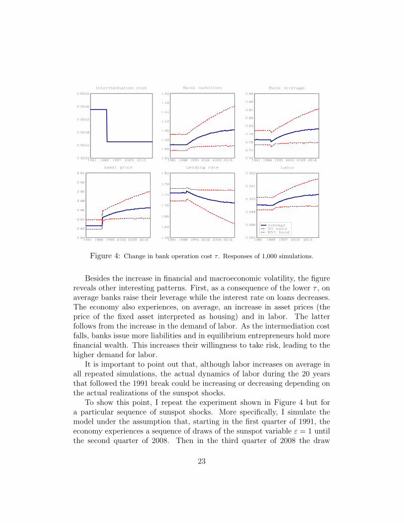
Figure 4: Change in bank operation cost τ . Responses of 1,000 simulations.

Besides the increase in financial and macroeconomic volatility, the figurereveals other interesting patterns. First, as a consequence of the lower τ , onaverage banks raise their leverage while the interest rate on loans decreases.The economy also experiences, on average, an increase in asset prices (theprice of the fixed asset interpreted as housing) and in labor. The latterfollows from the increase in the demand of labor. As the intermediation costfalls, banks issue more liabilities and in equilibrium entrepreneurs hold morefinancial wealth. This increases their willingness to take risk, leading to thehigher demand for labor.

It is important to point out that, although labor increases on average inall repeated simulations, the actual dynamics of labor during the 20 yearsthat followed the 1991 break could be increasing or decreasing depending onthe actual realizations of the sunspot shocks.

To show this point, I repeat the experiment shown in Figure 4 but fora particular sequence of sunspot shocks. More specifically, I simulate themodel under the assumption that, starting in the first quarter of 1991, theeconomy experiences a sequence of draws of the sunspot variable ε = 1 untilthe second quarter of 2008. Then in the third quarter of 2008 the draw

23

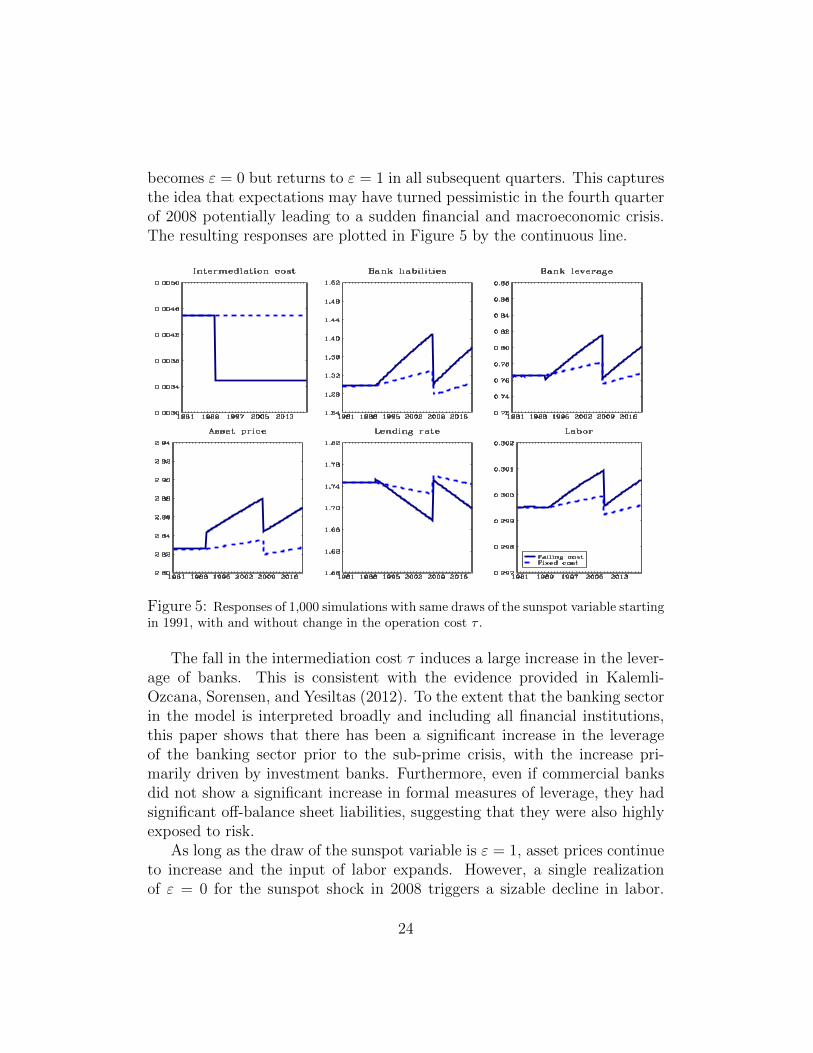
becomes ε = 0 but returns to ε = 1 in all subsequent quarters. This capturesthe idea that expectations may have turned pessimistic in the fourth quarterof 2008 potentially leading to a sudden financial and macroeconomic crisis.The resulting responses are plotted in Figure 5 by the continuous line.

Figure 5: Responses of 1,000 simulations with same draws of the sunspot variable startingin 1991, with and without change in the operation cost τ .

The fall in the intermediation cost τ induces a large increase in the lever-age of banks. This is consistent with the evidence provided in Kalemli-Ozcana, Sorensen, and Yesiltas (2012). To the extent that the banking sectorin the model is interpreted broadly and including all financial institutions,this paper shows that there has been a significant increase in the leverageof the banking sector prior to the sub-prime crisis, with the increase pri-marily driven by investment banks. Furthermore, even if commercial banksdid not show a significant increase in formal measures of leverage, they hadsignificant off-balance sheet liabilities, suggesting that they were also highlyexposed to risk.

As long as the draw of the sunspot variable is ε = 1, asset prices continueto increase and the input of labor expands. However, a single realizationof ε = 0 for the sunspot shock in 2008 triggers a sizable decline in labor.

24

Furthermore, even if the negative shock is only for one period and there areno crises afterwards, the recovery in the labor market is very slow. This isbecause the crisis generates a large decline in the financial wealth of employersand it takes a long time for them to rebuilt the lost wealth with savings.

Another way to show the importance of financial innovations for macroe-conomic stability, is to conduct the following exercise. I repeat the simulationof the model in response to the same sequence of sunspot draws but underthe assumption that τ does not change, that is, it remains at the pre-1991value after 1991. This counterfactual exercise illustrates how different the fi-nancial and macroeconomic dynamics in response to the same shocks wouldhave been in absence of financial innovations. The resulting simulation isshown in Figure 5 by the dash line.

As can be seen, without the change in τ , the same sequence of sunspotshocks would have generated a much smaller financial expansion before 2008as well as a much smaller financial and macroeconomic contraction in thethird quarter of 2008. Therefore, financial innovations could have contributedto the observed expansion of the financial sector in industrialized countriesbut it also created the conditions for greater financial and macroeconomicfragility that became evident only after the crisis materialized.

Downward wage rigidity Although the re-adjustment in financial vari-ables shown in Figure 5 is quite large, the response of labor is relatively small.The reason is because the decline in the demand for labor caused by the crisisis counterbalanced by a significant reduction in the wage rate. However, ifwages cannot fall because of downward rigidity, the response of labor couldbe much bigger. To show this, I now consider downward wage rigidities.

Suppose that wages are perfectly flexible only when the demand of laborinduces an increase in the wage or a moderate decline. More specifically, givenwt−1 the equilibrium real wage at t−1, the current wage wt must satisfy wt ≥ρwt−1. The coefficient ρ determines the degree of downward rigidity. Withρ = 1 wages never decline. With ρ = 0 wages are perfectly flexible. Although‘nominal’ wage rigidity is a more common feature of the economy, downward‘real’ rigidity should be interpreted as capturing downward nominal rigiditywhen inflation is very close to zero.

Denote by wt the wage rate that equalizes the demand and supply oflabor, that is, φt(wt)Bt =

(wtα

)ν. Equilibrium employment is always equal to

25

the demand, Ht = φt(wt)Bt, with the wage rate given by

wt =

wt, if wt ≥ ρwt−1

ρwt−1, if wt < ρwt−1

(16)

Figure 6 plots the simulation with ρ = 0.9999. As can be seen, the crisisinduces a drop in labor that is more than 7 percent (continuous line). With-out the change in τ , the drop in labor is also sizable but significantly smallerthan in the case with lower τ . Therefore, the combination of higher leveragescaused by the reduction in the intermediation cost together with downwardwage rigidities could create the conditions for more severe macroeconomiccontractions in response to a banking crisis.

Figure 6: Model with downward wage rigidity. Responses of 1,000 simulations with samedraws of the sunspot variable starting in 1991, with and without change in the operationcost τ .

4 Government debt

The analysis conducted so far shows that, due to market incompleteness andthe limited creation of financial assets, the equilibrium is inefficient. More

26

specifically, the premium over the wage that entrepreneurs require to hirelabor represents a wedge that distorts the labor market. If markets werecomplete, producers would be able to insure the idiosyncratic risk with thepurchase of state contingent claims and the wedge would be zero. But in theenvironment presented in this paper the only way for producers to achieveconsumption smoothing (by insuring the risk) is by holding financial assetsthat cannot be contingent on the idiosyncratic risk. Since the supply of theseassets is limited, the equilibrium is inefficient.

Given the limited ability of the financial sector to create financial assets,it is natural to ask whether the government could obviate this limitation byissuing public debt. In principle this could provide additional financial assetsheld by producers and could reduce the labor wedge. In this section I willshow that the ability of public debt to improve the equilibrium depends onhow the burden of the debt is financed.6

4.1 Public debt and taxation

After issuing public debt, the government has to pay the interests that matureon the debt with taxes. It becomes then important what type of taxes areused to fund the burden of debt. I will consider four types of taxes:

1. Lump-sum taxes on entrepreneurs.

2. Lump-sum taxes on workers.

3. Profit taxes on entrepreneurs.

4. Wage taxes on workers.

As we will see, public debt would unambiguously improve real allocationsonly if the burden of public debt is financed with lump-sum taxes on workers.

6There are other mechanisms that could generate financial assets held for insurancepurposes. Money, for example, could also play this role as in Brunnermeier and Sannikov(2016). In this paper money is a bubble that agents are willing to hold because of theinsurance it provides. More generally, bubbles like those considered in Miao and Wang(2011) could also play this role. In my framework, however, the reason entrepreneurswould hold bubbles is not because they relax the borrowing constraints (as in Miao andWang (2011)) but because they provide insurance.

27

Lump-sum taxes on entrepreneurs: The following proposition estab-lishes that with lump-sum taxes paid by entrepreneurs, public debt is irrele-vant for real sector of the economy (Ricardian equivalence).

Proposition 4.1 If the government uses lump-sum taxes charged only toentrepreneurs, then public debt does not affect real allocations.

To illustrate this result, consider first the government budget constraint,

Tt = Dt −Dt+1

Rbt

,

where Tt denotes the lump-sum taxes charged to entrepreneurs and Dt is thegovernment debt due at time t and Dt+1 is the new debt due at t + 1. Forsimplicity I am abstracting from the possibility that banks could default sothat in equilibrium the interest rate on government bonds must be equal tothe interest rate on bank liabilities, Rb

t . This implies that for entrepreneursbank liabilities are equivalent to government liabilities.

Let’s consider now the budget constraint for entrepreneurs,

cit +bit+1

Rbt

+dit+1

Rbt

+ Tt = (zit − wt)hit + bit + dt,

where dit is the individual debt held by entrepreneur i. Eliminating Tt usingthe government budget constraint, the budget constraint for an individualentrepreneur i can be rewritten as

cit +bit+1

Rbt

= (zit − wt)hit + bit,

where bit = bit + dit −Dt.The resulting budget constraint has the same structure as the budget

constraint without government debt. The only difference is that bit has beenreplaced with bit. Therefore, the solution is still given by Lemma 2.1 andtakes the form

hit = φ(wt)bit.

Again, the only difference is that now we have bit instead of bit. Using theindividual demands for labor, we can then derive the aggregate demand

Ht = φ(wt)

∫bit = φ(wt)

∫ (bit + dit −Dt

)= φ(wt)Bt.

28

The last equality derives from the fact that the sum of the public debt held byall entrepreneurs is equal to the aggregate public debt. Thus, the aggregatedemand for labor is unaffected by the issuance of public debt but dependsonly on the liabilities issued by the financial intermediation sector, Bt.

This result has a simple intuition. Even though the public debt will beheld by entrepreneurs and it represents a financial asset for them, this istotally offset by the tax liabilities that they have to pay. As a result, sincetheir net wealth (net of the tax liabilities) does not change, their economicdecisions are unaffected (Ricardian equivalence).

Lump-sum taxes on households: If the government finances the burdenof public debt with lump-sum taxes on households, then effectively the gov-ernment borrows on behalf of households (Azzimonti and Quadrini (2014)).In this case public debt improves allocations as stated by the following propo-sition.

Proposition 4.2 If the government uses lump-sum taxes charged only tohouseholds, then higher public debt is associated with higher average employ-ment and output and lower macroeconomic volatility.

The intuitive proof follows the same steps of the proof provided abovestarting with the budget constraint of entrepreneurs

cit +bit+1

Rbt

+dit+1

Rbt

= (zit − wt)hit + bit + dt.

The only difference is that now entrepreneurs do not pay taxes Tt. We canagain rewrite the budget constraint as

cit +bit+1

Rbt

= (zit − wt)hit + bit,

where now bit = bit + dit (there is not Dt).The resulting budget constraint has the same structure as the budget

constraint without government debt and the solution is still given by Lemma2.1. In particular, the demand for labor is given by

hit = φ(wt)bit.

29

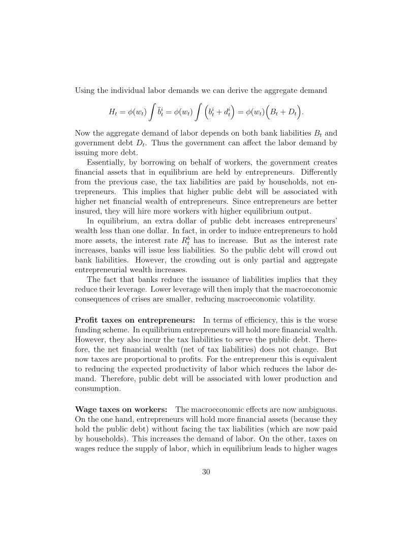
Using the individual labor demands we can derive the aggregate demand

Ht = φ(wt)

∫bit = φ(wt)

∫ (bit + dit

)= φ(wt)

(Bt +Dt

).

Now the aggregate demand of labor depends on both bank liabilities Bt andgovernment debt Dt. Thus the government can affect the labor demand byissuing more debt.

Essentially, by borrowing on behalf of workers, the government createsfinancial assets that in equilibrium are held by entrepreneurs. Differentlyfrom the previous case, the tax liabilities are paid by households, not en-trepreneurs. This implies that higher public debt will be associated withhigher net financial wealth of entrepreneurs. Since entrepreneurs are betterinsured, they will hire more workers with higher equilibrium output.

In equilibrium, an extra dollar of public debt increases entrepreneurs’wealth less than one dollar. In fact, in order to induce entrepreneurs to holdmore assets, the interest rate Rb

t has to increase. But as the interest rateincreases, banks will issue less liabilities. So the public debt will crowd outbank liabilities. However, the crowding out is only partial and aggregateentrepreneurial wealth increases.

The fact that banks reduce the issuance of liabilities implies that theyreduce their leverage. Lower leverage will then imply that the macroeconomicconsequences of crises are smaller, reducing macroeconomic volatility.

Profit taxes on entrepreneurs: In terms of efficiency, this is the worsefunding scheme. In equilibrium entrepreneurs will hold more financial wealth.However, they also incur the tax liabilities to serve the public debt. There-fore, the net financial wealth (net of tax liabilities) does not change. Butnow taxes are proportional to profits. For the entrepreneur this is equivalentto reducing the expected productivity of labor which reduces the labor de-mand. Therefore, public debt will be associated with lower production andconsumption.

Wage taxes on workers: The macroeconomic effects are now ambiguous.On the one hand, entrepreneurs will hold more financial assets (because theyhold the public debt) without facing the tax liabilities (which are now paidby households). This increases the demand of labor. On the other, taxes onwages reduce the supply of labor, which in equilibrium leads to higher wages

30

and lower employment. Which of the two effects dominate depends on theelasticity of the labor supply. If the supply of labor is sufficiently elastic, thesecond effect dominates and the equilibrium will be characterized by loweremployment and output. However, aggregate volatility may be lower. This isbecause the higher supply of bonds increases the interest rate which in turnwill be associated with lover bank leverage.

4.2 Discussion

The above analysis suggests that, provided that the government uses the‘right’ taxes to fund the debt burden, public debt could be welfare improving.This conclusion, however, ignores political feasibility. First, lump-sum taxesare difficult to use in practice because households earn different incomes.So, only proportional or progressive taxes are feasible. But then, whichproportional taxes, the optimality of debt is no longer guaranteed.

The second consideration is time consistency. It may be possible that is-suing debt and later taxing households is ex-ante optimal. But once the debthas been issued and households have to pay it, they may have an incentiveto lobby the government to default on the debt. Default can take differentforms, not necessarily outright repudiation. One less direct form of defaultis to shift the taxation burden from households to entrepreneurs. Providedthat households have sufficient political power, this is likely to happen. So weend up again in a situation in which the net financial wealth of entrepreneurs(public debt minus the tax liabilities) does not change. This is likely to beanticipated when the government issues the debt in the first place, whichneutralizes the positive effects of issuing public debt.

To conclude, public debt could improve the equilibrium allocation if as-sociated with the proper taxation scheme. In practise, the ‘proper’ taxationscheme may not be feasible or credible. This limits the role of public debt asa way to complete the market and improve real allocations.

5 Conclusion

The traditional role of banks is to facilitate the transfer of resources fromagents in excess of funds to agents in need of funds. This paper emphasizesa second important role played by banks: the issuance of liabilities that canbe held by the nonfinancial sector for insurance purposes. This is similarto the role of banks in creating liabilities that can be used for transaction

31

as in Williamson (2012). The difference is that in the current paper bankliabilities are valued not for their use as a mean of exchange but as an insur-ance instrument. When the stock of bank liabilities or their value are low,agents are less willing to engage in risky economic activities and this causesa macroeconomic downturn.

The paper also shows that booms and busts in financial intermediationcan be driven by self-fulfilling expectations about the liquidity of banks.When the economy expects the banking sector to be liquid, banks have anincentive to leverage and this generates a macroeconomic boom. But asthe leverage increases, the banking sector becomes vulnerable to pessimisticexpectations that could generate self-fulfilling liquidity crises.

The model has been used to study the impact of financial innovations onfinancial and macroeconomic stability. Financial innovations can generatea macroeconomic expansion but could also increase the potential instabilityof the macro-economy. As long as expectations remain optimistic, coun-tries experience a macroeconomic boom. However, when expectations turnpessimistic, the economy experiences deeper macroeconomic contractions.

Can the issuance of government debt improve the allocation of resourcesand reduce the probability and/or the macroeconomic consequences of crises?The paper has shown that the issuance of pubic debt could play a role inthis regard but only if associated to a specific taxation scheme. The ‘right’taxation scheme, however, may not be politically feasible or credible.

32

Appendix

A Proof of Lemma 2.1

The optimization problem of an entrepreneur can be written recursively as

Vt(bt) = maxht

EtVt(at) (17)

subject to

at = bt + (zt − wt)ht

Vt(at) = maxbt+1

{ln(ct) + βEtVt+1(bt+1)

}(18)

subject to

ct = at −bt+1

Rt

Since the information set changes from the beginning of the period to theend of the period, the optimization problem has been separated according to theavailable information. In sub-problem (17) the entrepreneur chooses the input oflabor without knowing the productivity zt. In sub-problem (18) the entrepreneurallocates the end of period wealth in consumption and savings after observing zt.

The first order condition for sub-problem (17) is

Et∂Vt∂at

(zt − wt) = 0.

The envelope condition from sub-problem (18) gives

∂Vt∂at

=1

ct.

Substituting in the first order condition we obtain

Et(zt − wtct

)= 0. (19)

At this point we proceed by guessing and verifying the optimal policies foremployment and savings. The guessed policies take the form:

ht = φtbt (20)

ct = (1− β)at (21)

33

Since at = bt + (zt − wt)ht and the employment policy is ht = φtbt, the endof period wealth can be written as at = [1 + (zt − wt)φt]bt. Substituting in theguessed consumption policy we obtain

ct = (1− β)[1 + (zt − wt)φt

]bt. (22)

This expression is used to replace ct in the first order condition (19) to obtain

Et[

zt − wt1 + (zt − wt)φt

]= 0, (23)

which is the condition stated in Lemma 2.1.To complete the proof, we need to show that the guessed policies (20) and (21)

satisfy the optimality condition for the choice of consumption and saving. This ischaracterized by the first order condition of sub-problem (18), which is equal to

− 1

ctRt+ βEt

∂Vt+1

∂bt+1= 0.

From sub-problem (17) we derive the envelope condition ∂Vt/∂bt = 1/ct which canbe used in the first order condition to obtain

1

ct= βRtEt

1

ct+1.

We have to verify that the guessed policies satisfy this condition. Using theguessed policy (21) and equation (22) updated one period, the first order conditioncan be rewritten as

1

at= βRtEt

1

[1 + (zt+1 − wt+1)φt+1]bt+1.

Using the guessed policy (21) we have that bt+1 = βRtat. Substituting andrearranging we obtain

1 = Et[

1

1 + (zt+1 − wt+1)φt+1

]. (24)

The final step is to show that, if condition (23) is satisfied, then condition(24) is also satisfied. Let’s start with condition (23), updated by one period.Multiplying both sides by φt+1 and then subtracting 1 in both sides we obtain

Et+1

[(zt+1 − wt+1)φt+1

1 + (zt+1 − wt+1)φt+1− 1

]= −1.

Multiplying both sides by -1 and taking expectations at time t we obtain (24).

34

B Proof of Proposition 2.1

As shown in Lemma 2.1, the optimal saving of entrepreneurs takes the formbit+1/R

bt = βait, where ait is the end-of-period wealth ait = bit + (zit − wt)h

it.

Since hit = φ(wt)bit (see Lemma 2.1), the end-of-period wealth can be rewritten

as ait = [1 + (zit − wt)φ(wt)]bit. Substituting into the optimal saving and aggregat-

ing over all entrepreneurs we obtain

Bt+1 = βRbt

[1 + (z − wt)φ(wt)

]Bt. (25)

This equation defines the aggregate demand for bonds as a function of theinterest rate Rbt , the wage rate wt, and the beginning-of-period aggregate wealthof entrepreneurs Bt. Notice that the term in square brackets is bigger than 1.Therefore, in a steady state equilibrium where Bt+1 = Bt, the condition βR < 1must be satisfied.

Using the equilibrium condition in the labor market, I can express the wage rateas a function of Bt. In particular, equalizing the demand for labor, HD

t = φ(wt)Bt,to the supply from households, HS

t = (wt/α)ν , the wage wt can be expressed asa function of only Bt. We can then use this function to replace wt in (25) andexpress the demand for bank liabilities as a function of only Bt and Rbt as follows

Bt+1 = s(Bt)Rbt . (26)

The function s(Bt) is strictly increasing in the wealth of entrepreneurs, Bt.Consider now the supply of bonds from households. For simplicity I assume

that η = 0 in the borrowing constraint (2). Therefore, this constraint takes theform lt+1 ≤ κ. Using this limit together with the first order condition (4), we havethat, either the interest rate satisfies 1 = βRbt or households are financially con-strained, that is, Bt+1 = κ. When the interest rate is equal to the inter-temporaldiscount rate (first case), we can see from (25) that Bt+1 > Bt. So eventually, theborrowing constraint of households becomes binding, that is, Bt+1 = κ (secondcase). When the borrowing constraint is binding, the multiplier µt is positive andcondition (4) implies that the interest rate is smaller than the inter-temporal dis-count rate. So the economy has reached a steady state. The steady state interestrate is determined by condition (26) after setting Bt = Bt+1 = κ. This is the onlysteady state equilibrium.

When η > 0 in the borrowing constraint (2), the proof is more involved butthe economy also reaches a steady state with βR < 1.

35

C First order conditions for households

The optimization problem of a household can be written recursively as

Vt(lt, kt) = maxht,lt+1,kt+1

ct − α h1+ 1

νt

1 + 1ν

+ βVt+1(lt+1, kt+1)

subject to

ct = wtht + χkt +lt+1

Rlt− lt − (kt+1 − kt)pt

η ≥ lt+1.

Given βµt the lagrange multiplier associated with the borrowing constraint,the first order conditions with respect to ht, lt+1, kt+1 are, respectively,

−αh1νt + wt = 0,

1

Rlt+ β

∂Vt+1(lt+1, kt+1

∂lt+1− βµt = 0,

−pt + β∂Vt+1(lt+1, kt+1

∂kt+1+ ηβµtEtpt+1 = 0.

The envelope conditions are

∂Vt(lt+1, kt+1

∂lt+1= −1,

∂Vt(lt+1, kt+1

∂kt+1= χ+ pt.

Updating by one period and substituting in the first order conditions we obtain(3), (4), (5).

D First order conditions for problem (9)

The probability of renegotiation, denoted by θt+1, is defined as

θt+1 =

0, if ωt+1 < ξ

λ, if ξ ≤ ωt+1 ≤ 1

1, if ωt+1 > 1

36

Define β(1−θt+1)γt the Lagrange multiplier associated to the constraint bt+1 ≤lt+1. The first order conditions for problem (9) with respect to bt+1 and lt+1 are

1− ϕtRbt

Et∂bt+1

∂bt+1− ∂ϕt∂bt+1

Etbt+1

Rbt

− βEt∂bt+1

∂bt+1− β(1− θt+1)γt = 0, (27)

− 1

Rlt+

1− ϕtRbt

Et∂bt+1

∂lt+1− ∂ϕt∂lt+1

Etbt+1

Rbt

+ βEt

(1− ∂bt+1

∂lt+1

)+ β(1− θt+1)γt = 0.

(28)

I now use the definition bt+1 provided in (6) to derive the following terms

∂ϕt∂bt+1

= ϕ′t+1

1

lt+1,

∂ϕt∂lt+1

= −ϕ′t+1ωt+11

lt+1,

Et∂bt+1

∂bt+1= 1− θt+1,

Et∂bt+1

∂lt+1= θt+1ξ,

Etbt+1 = (1− θt+1)bt+1 + χt+1ξlt+1.

Substituting in (27) and (28) and re-arranging we obtain

1

Rbt

= β

[1 +

ϕt+1 + ϕ′t+1ωt+1 + γt

1− ϕt+1 − ϕ′t+1ωt+1

], (29)

1

Rlt= β

[1 +

ϕ′t+1ω2t+1(1− θt+1)(1 + γt)

1− ϕt+1 − ϕ′t+1ωt+1+(

1− θt+1 + θt+1ξ)γt

], (30)

where ωt+1 = ωt+1 +θt+1ξ

1−θt+1.

The multiplier γt is zero if ωt+1 < 1 and positive if ωt+1 = 1. Therefore, thefirst order conditions can be written as

1

Rbt

= β

[1 +

ϕt+1 + ϕ′t+1ωt+1

1− ϕt+1 − ϕ′t+1ωt+1

],

1

Rlt= β

[1 +

ϕ′t+1ω2t+1(1− θt+1)

1− ϕt+1 − ϕ′t+1ωt+1

],

which are satisfied with the inequality sign if γt > 0. Since they are all functionsof ωt+1, the first order conditions can be written as in (10) and (11).

37

E Proof of Lemma 2.2

Let’s consider the first order conditions (29) and (30) when ωt+1 < 1. In this casethe lagrange multiplier γt is zero. Since At+1 > 0 and ϕt+1 and ϕ′t+1 are both

positive for ωt+1 > ξ, conditions (29) and (30) imply that Rbt and Rlt are smaller

than 1/β.The next step is to derive the return spread from (29) and (30) to obtain

Rlt

Rbt

=1

1− ϕt+1 − ϕ′t+1At+1[1− (1− θt+1)At+1]. (31)

Given the properties of the cost function (Assumption 1), to show that thespread is bigger than 1 I only need to show that (1 − θt+1)At+1 < 1. Using

At+1 = ωt+1 +θt+1ξ

1−θt+1and taking into account that ωt+1 < 1 and θt+1 < 1, we can

verify that (1− θt+1)At+1 < 1. Therefore, the spread is bigger than 1.To show that the spread is increasing in the leverage, I differentiate (31) with

respect to ωt+1 to obtain

Rlt

Rbt

=(ϕ′′t+1At+1 + 2ϕ′t+1)[1− (1− θt+1)At+1][

1− ϕt+1 − ϕ′t+1At+1(1− (1− θt+1)At+1

]2Given the properties of the cost function (Assumption 1), the derivative is zero

for ωt+1 ≤ ξ. To prove that the derivative is positive for ωt+1 > ξ, I only need toshow that (1 − θt+1)At+1 < 1, which has already been shown above. Therefore,the return spread is strictly increasing for ωt+1 > ξ.

F Proof of Proposition 2.2

Banks make decisions at two different stages. At the beginning of the period theychoose whether to renegotiate the debt and at the end of the period they choose thefunding and lending policies. Given the initial states, bt and lt, the renegotiationdecision boils down to a take-it or leave-it offer made by each bank to its creditorsfor the repayment of the debt. Denote by bt = f(bt, lt, ξ

et ) the offered repayment.

This depends on the individual liabilities bt, individual assets lt, and the expectedliquidation price of assets ξet . The superscript e is to make clear that the bankdecision depends on the expected price in the eventuality of liquidation. Obviously,the best repayment offer made by the bank is

f(bt, lt, ξet ) =

bt, if bt ≤ ξet lt

ξet lt, if bt > ξet lt

, (32)

38

which is accepted by creditors whenever the actual liquidation price is bigger thanthe expected price ξet .

After the renegotiation stage, banks choose the funding and lending policies,

bt+1 and lt+1. These policies depend on the two interest rates, Rbt and Rl, and

on the probability distribution of the next period liquidation price ξt+1. Since wecould have multiple equilibria, the next period price could be stochastic. Supposethat the price could take two values, ξ and 1, with the probability of the low valuedefined as

θ(ωt+1) =

0, if ωt+1 < ξ

λ, if ξ ≤ ωt+1 ≤ 1

1, if ωt+1 > 1.

The variable ωt+1 = bt+1/lt+1 represents the leverage of all banks in a sym-metric equilibrium, that is, they all choose the same leverage. For the moment thesymmetry of the equilibrium is an assumption. I will then show below that in factbanks do not have incentives to deviate from the leverage chosen by other banks.

Given the above assumption about the probability distribution of the liqui-dation price, the funding and lending policies of the bank are characterized in

Lemma 2.2 and depend on Rbt and Rlt. In short, if R

bt/(1 − τ) = Rlt, then the

optimal policy of the bank is to choose a leverage ωt+1 ≤ ξ. If Rbt/(1 − τ) < Rlt,

the optimal leverage is ωt+1 > ξ.Given the assumption that the equilibrium is symmetric (all banks choose the

same leverage ωt+1), multiple equilibria arise if the chosen leverage is ωt+1 ∈ {ξ, 1}.In fact, once we move to the next period, if the market expects ξet+1 = ξ, all banksare illiquid and they choose to renege on their liabilities (given the renegotiationpolicy (32)). As a result, there will not be any bank that can buy the liquidatedassets of other banks. Then the only possible price that is consistent with theexpected price is ξt+1 = ξ. On the other hand, if the market expects ξet+1 = 1,banks are liquid and, if one bank reneges, creditors can sell the liquidated assetsto other banks at the price ξt+1 = 1. Therefore, it is optimal for banks not torenegotiate consistently with the renegotiation policy (32).

The above proof, however, assumes that the equilibrium is symmetric, that is,all banks choose the same leverage. To complete the proof, we have to show thatthere is no incentive for an individual bank to deviate from the leverage chosen byother banks. In particular, I need to show that, in the anticipation that the nextperiod liquidation price could be ξt+1 = ξ, a bank do not find convenient to chosea lower leverage so that, in the eventuality that the next period price is ξt+1 = ξ,the bank could purchase the liquidated asset at a price lower than 1 and make aprofit (since the unit value for the bank of the liquidated assets is 1.

39

If the price at t+ 1 is ξt+1 = ξ, a liquid bank could offer a price ξ + ε, where εis a small but positive number. Since the repayment offered by a defaulting bankis ξlt+1, creditors prefer to sell the assets rather than accepting the repaymentoffered by the defaulting bank. However, if this happens, the expectation of theliquidation price ξe = ξ turns out to be incorrect ex-post. Therefore, the presenceof a single bank with liquidity will raise the expected liquidation price to ξ + ε.But even with this new expectation, a bank with liquidity can make a profit byoffering ξ + 2ε. Again, this implies that the expectation turns out to be incorrectex-post. This mechanism will continue to raise the expected price to ξet+1 = 1.At this point the liquid bank will not offer a price bigger than 1 and the ex-postliquidation price is correctly predicted to be 1. Therefore, as long as there is asingle bank with liquidity, the expected liquidation price must be 1. But then abank cannot make a profit in period t+ 1 by choosing a lower leverage in period twith the goal of remaining liquid in the next period. This proves that there is noincentive to deviate from the policy chosen by other banks.

Finally, the fact that multiple equilibria cannot arise when ωt < ξ is obvious.Even if the price is ξ, banks remain liquid.

G Proof of Proposition 2.3

Given a fixed interest rate Rb, the aggregate demand for bank liabilities, equation(13), has a converging fix point B∗(Rb). The fixed point is increasing in Rb andconverges to infinity as Rb converges to 1/β. This implies that, if τ = 0, thenthe leverage of banks is always bigger than ξ. To show this, suppose that bankschoose a leverage of ω < ξ. According to conditions (10) and (11), we have that

Rb = Rl = 1/β. But when Rb = 1/β the demand of bank liabilities is unboundedin the limit. This implies that to reach a stable equilibrium without renegotiation(that is, ω < ξ), Rb must be smaller than 1/β. This requires τ to be sufficiently

big. In fact, when τ > 0 and ω < ξ, we have Rb/(1 − τ) = Rl = 1/β. Since the

demand for bank liabilities is increasing in Rb, there must be some τ > 0 suchthat, for τ > τ , the equilibrium is characterized by ω < ξ. This implies thatthe economy is not subject to crises and converges to a steady state. For τ < τ ,instead, the equilibrium is characterized by ω > ξ. In this case the economy issubject to self-fulfilling crises and, therefore, it does not converge to a steady state.

H Numerical solution

I describe first the numerical procedure without the structural break. I will thendescribe the numerical procedure when τ changes inducing a transition dynamics.

40

H.1 Stationary equilibrium without structural break

The states of the economy are given by the bank liabilities Bt, the bank loansLt and the realization of the sunspot shock εt. These three variables are impor-tant in determining the renegotiation liabilities Bt. However, once we know therenegotiated liabilities Bt, this becomes the sufficient state for solving the model.Therefore, in the computation I will solve for the recursive equilibrium using Btas a state variable.

I will use the following equilibrium conditions:

Ht = φ(wt)Bt, (33)

Bt+1

Rbt= βAt, (34)

At = Bt + (1− wt)Ht (35)

αH1νt = wt, (36)

1 = βRlt(1 + µt), (37)

pt = βEt[χ+ (1 + ηµt)pt+1

], (38)

Lt+1 = ηEtpt+1, (39)

1

Rbt

= β

[1 +

ϕt+1 + ϕ′t+1ωt+1

1− ϕt+1 − ϕ′t+1ωt+1

], (40)

1

Rlt= β

[1 +

ϕ′t+1ω2t+1(1− θt+1)

1− ϕt+1 − ϕ′t+1ωt+1

], (41)

Rbt =

[1− θ(ωt+1) + θ(ωt+1)

(ξ

ωt+1

)]Rbt , (42)

ωt+1 =Bt+1

Lt+1(43)

Equations (33)-(35) come from the aggregation of the optimal policies of en-trepreneurs (labor demand, savings and end of periods wealth). Equations (36)-(39) come from the optimization problem of households (labor supply, optimalborrowing, optimal holding of the fixed asset, and borrowing constraint). Noticethat the borrowing constraint of households (equation (39) is not always bind-ing. However, when it is not binding and the multiplier is µt = 0, households’borrowing is not determined. Therefore, without loss of generality I assume thatin this case households borrow up to the limit. This explains why the borrowingconstraint is always satisfied with equality. Equations (40)-(41) are the first order

41

conditions of banks. These conditions are satisfied with equality if ωt+1 < 1 andwith inequality if ωt+1 = 1. Equation (42) defines the expected return on bankliabilities given the price of these liabilities, that is, the inverse of Rbt . The finalequation (43) simply defines leverage.

One complication in solving this system of equations is that the expectation ofthe next period price of the fixed asset, Etpt+1, is unknown. All we know is thatthe next period price is a function of Bt+1, that is, pt+1 = P (Bt+1). If I knewthe function P (Bt+1), for any given state Bt, the above conditions would be a

system of 11 equations in 11 variables: Ht, At, µt, wt, pt, Rbt , R

lt, R

bt , Bt+1, Lt+1,

ωt+1. Notice that Bt+1 is a known function of Bt+1, Lt+1 and the realization ofthe sunspot shock ε. Therefore, I can compute the expectation of the next periodprice pt+1 if I know the function P (Bt+1). We can then solve the 11 equations forthe 11 variables and this would provide a solution for any given state Bt.

The problem is that I do not know the function P (Bt+1). Therefore, theprocedure will be based on a parametrization of an approximation of this function.In particular, I approximate P (Bt+1) with a piece-wise linear function over a gridfor the state variable Bt. I then solve the above system of equations at each gridpoint for Bt. As part of the solution I obtain the current price pt. I then use thesolution for the current price to update the approximated function P (Bt+1) at thegrid point. I repeat the iteration until convergence, that is, the values guessed forP (Bt+1) at each grid point must be equal (up to a small rounding number) to thevalues of pt obtained by solving the model (given the guess for P (Bt+1)).

H.2 Equilibrium with structural break

When the intermediation cost τ changes, the economy transits from a stochas-tic equilibrium to a new stochastic equilibrium. This requires to solve for thetransition and the solution method is based on the following steps.

1. I first compute the stochastic equilibrium under the regime that proceedsthe structural break (the operation cost of banks is constant at the initiallevel).

2. I then compute the stochastic equilibrium under the terminal regime (theoperation cost of banks remains constant at the new level).

3. At this point I solve the model backward at any time t starting at the termi-nal period when the operation cost remain constant at the new level. At eacht I solve the system (33)-(43) using the approximated function Pt+1(Bt+1)found at time t + 1. In the first backward step (last period of the transi-tion), Pt+1(Bt+1) is the approximated price function found in the stochasticstationary equilibrium after the break (see previous computational step).

42

References

Adrian, T., Colla, P., & Shin, H. S. (2013). Which Financial Frictions?Parsing the Evidence from the Financial Crisis of 2007-9. In Acemoglu,D., Parker, J., & Woodford, M. (Eds.), NBER Macroeconomics Annual2012, pp. 159 – 214. MIT Press, Cambridge, Massachusetts.

Arellano, C., Bai, Y., & Kehoe, P. (2011). Financial Markets and Fluc-tuations in Uncertainty. Research Department Staff Report, FederalReserve Bank of Minneapolis.

Bernanke, B., & Gertler, M. (1989). Agency Costs, Net Worth, and BusinessFluctuations. American Economic Review, 79 (1), 14–31.

Boissay, F., Collard, F., & Smets, F. (2010). Booms and Systemic BankingCrises. Unpublished manuscript, European Central Bank.

Brunnermeier, M., & Sannikov, Y. (2014). A Macroeconomic Model with aFinancial Sector. American Economic Review, 104 (2), 379–421.

Brunnermeier, M., & Sannikov, Y. (2016). On the Optimal Inflation Rate.Unpublished manuscript, Princeton University.

Cole, H. L., & Kehoe, T. J. (2000). Self-Fulfilling Debt Crises. Review ofEconomic Studies, 67 (1), 91–116.

Corbae, D., & D’Erasmo, P. (2012). A Quantitative Model of Banking In-dustry DYnamics. Unpublished manuscript, University of Wisconsinand University of Maryland.

De Fiore, F., & Uhlig, H. (2011). Bank Finance versus Bond Finance. Journalof Money Credit and Banking, 43 (7), 1399–1421.

Eisfeldt, A., & Muir, T. (2012). Aggregate Issuance and Savings Waves.Unpublished manuscript, Anderson School of Management, UCLA.

Gertler, M., & Kiyotaki, N. (2010). Financial Intermediation and CreditPolicy in Business Cycle Analysis. In Friedman, B. M., & Woodford,M. (Eds.), Handbook of Monetary Economics, Vol. 3, chap. 11, pp.1341–96. Elsevier, Amsterdam: Elsevier Science.

43

Gertler, M., & Karadi, P. (2011). A Model of Unconventional MonetaryPolicy. Journal of Monetary Economics, 58 (1), 17–34.

Holmstrom, B., & Tirole, J. (1997). Financial Intermediation, LoanableFunds, and the Real Sector. Quarterly Journal of Economics, 112 (3),663–91.

Kalemli-Ozcana, S., Sorensen, B., & Yesiltas, S. (2012). Leverage AcrossFirms, Banks, and Countries. Journal of International Economics,88 (2), 284–298.

Kiyotaki, N., & Moore, J. H. (1997). Credit Cycles. Journal of PoliticalEconomy, 105 (2), 211–48.

Meh, C. A., & Moran, K. (2010). The Role of Bank Capital in the Propa-gation of Shocks. Journal of Economic Dynamics and Control, 34 (3),555–76.

Mendoza, E., & Quadrini, V. (2010). Financial Globalization, FinancialCrises and Contagion. Journal of Monetary Economics, 57 (1), 24–39.

Miao, J., & Wang, P. (2011). Bubbles and Credit Constraints. Unpublishedmanuscript, Boston University and Hong Kong University of Scienceand Technology.

Perri, F., & Quadrini, V. (2011). International Recessions. NBER WorkingPaper No. 17201.

Rampini, A., & Viswanathan, S. (2012). Financial Intermediary Capital.Unpublished manuscript, Duke University.

Shourideh, A., & Zetlin-Jones, A. (2012). External Financing and the Role ofFinancial Frictions over the Business Cycle: Measurement and Theory.Unpublished manuscript, Wharton School.

Van den Heuvel, S. J. (2008). The Welfare Cost of Bank Capital Require-ments. Journal of Monetary Economics, 55 (2), 298–320.

Williamson, S. D. (2012). Liquidity, Monetary Policy, and the Financial Cri-sis: A New Monetarist Approach. American Economic Review, 102 (6),2570–2605.

44