WP-2017-005

Center for Advanced Economic Study

Fukuoka University

(CAES)

8-19-1 Nanakuma, Jonan-ku, Fukuoka,

JAPAN 814-0180

Faculty of Economics

Fukuoka University

Bandwagon Effects and Local Monopoly Pricing

In Professional Team Sports Market.

J M Kang, Y. J. Ryu, Peng Liu

CAES Working Paper Series

1

Bandwagon Effects and Local Monopoly Pricing

in Professional Team Sports Market.

J. Moonwon Kang

Professor, Faculty of Economics, Fukuoka University, Japan.

Young Jin Ryu

Assistant Professor, Kitakyusyu City University, Japan

Peng Liu

Assistant Professor, Guangdong Ocean University, China.

Abstract:

This study establishes a case that bandwagon effects impart upward sloping segments to

market demand curves. As an example of such cases, we analyze a professional team

sports market characterized by local monopoly supply and demand induced by

bandwagon effects. Assuming consumers’ choice of attending the game is indivisible

and there exist systematic differences in loyalty to the local team among potential

attendants, we build a positive relation between ticket price and the number of entrants

to stadiums. We derive theoretical results that size of stadium does not affect the

optimum ticket pricing of monopoly team, and the strong of bandwagon effects is

associated with lower ticket prices. Further, we show that enlargements of stadium size

do not increase teams’ investments to team quality. A look at the evidence suggests our

theoretical results are largely consistent with real world observation in Japan and

Europe.

* This study is supported by the program for scientific research start-up funds of

Guangdong Ocean University.

2

Introduction

In his 1991 paper, Gary Becker suggested that, when individual demand is positively

related to the market demand, i.e., when there exist bandwagon effects in market

demand, the demand curve for the good is positively sloped for a wide range, and this

upward sloping demand curve could explain the well-observed and perpetuating

phenomenon of excess demand(queues to attend the successful sporting events) or

excess supply(vacancies in the stadium) in sports product markets. Becker suggested

that, if the pleasure from attending the game is greater when many people want to attend

the same event, the demand curve first rises and then falls, and combined with the fixed

supply(given number of seats in the stadium), the upward sloping demand curve would

be a source of excess demand or supply. This view, however, has been criticized by

Gisser et. al.(2009) who assert that Becker`s hypothesis of upward rising demand curve

is valid only when bandwagon effect is preposterously large, and is inconsistent with

standard empirical observations.

Both Becker’s hypothesis and criticism by Gisser et. al. and others(1) remain

unsatisfactory because these studies do not make clear the corresponding

utility-maximization and profit-maximization problems while discussing the possible

relations among bandwagon effect, demand curve and market outcome. The purpose of

the present study is to establish a sensible case wherein Becker’s hypothesis is valid,

and to examine its implications in sports product market.

The model we present here is based on the following basic assumptions: one, we

describe individual’s choice of attending a professional sport game and assume this

choice is indivisible(attend or not), two, loyalties to local sport team differ among

potential attendants to the game, and strong loyalty to the team yields higher utility from

the game, three, there exists bandwagon effect, which produces positive relation

between the number of attendants and pleasures obtained from attending the game, four,

the sport team under our investigation is a local monopoly and, in the short-run, the cost

of providing the game is constant regardless of the number of attendants.

This study is organized as follows: Section 2 describes the basic model and establishes

a case in which the demand for the sports game is positively related to ticket prices for a

wide range. In Section 3, we explain how local monopoly pricing of match day ticket is

affected by bandwagon effects in demand sides. We will derive a theoretical view that

3

the stadium size would have no influence to the optimum ticket pricing, which seems

largely consistent with real world observations in England Premier League and Japan

J-1 League. Section 4 extends the basic analysis to examine how changes in the strength

of bandwagon effect affect the ticket pricing and derives a result that strong bandwagon

effects will lower the monopoly price. We suggest a view that regional differences in

bandwagon effects could explain the wide discrepancies in match day ticket prices

observed among top leagues in European football. In Section 4, we further analyze the

possible relations among bandwagon effects, stadium sizes and investments in team’s

quality. We found that investments in team quality are not strongly related with stadium

sizes. Concluding remarks is given in Section 5.

Basic Framework

We assume the net surplus of the ith attendant to the game is(see L. Pepall and J.

Reiff(2016) among others for similar specification of utility function)

(1) {Ui = θiυ(nd) − λp

= 0

if attend the gameif not

where p is the ticket price, nd is the number of fans who want to attend the game with

the given ticket price p, and λ is the marginal utility of income which is assumed to be

identical to every individual. The parameter θi ∈ [0 1] ranks orders of population by

the intensity of their preference of the game(which would be related to their loyalty to

the team). We assume population is uniformly distributed on the line θ ∈ [0 1]. Thus,

normalizing total population n0 = 1 , the number of population whose preference

parameter θi is larger than θ̂ will be simply (1 − θ̂) (see Figure 1). It is important to

note that the utility associated with the game is defines as a function of nd, which is

not necessarily equal to actual number of attendants in our model as we will show

below(see footnote). We assume υ is a twice differentiable function and

υ′ =∂υ(nd)

∂nd> 0, ∙ υ′′ =

∂2υ(nd)

∂(nd)2< 0

4

FIGURE 1

Bandwagon effect, originally defined by Leibenstein(1950) as “the desire to join the

crowd, be ‘one of the boys`, etc. – phenomena of mob motivations and mass psychology

either in their grosser or more delicate aspects”, is captured in this model by the

assumption of υ′ > 0.

Define θi∗ as in (2),

(2) θi∗υ(nd) − λp = 0

then, it would be apparent that, for given ticket price p, those fans whose preference for

the game θi is larger than θi∗ will want to attend the game, and the following relation

holds,

(3) nd = 1 − θi∗.

From (2) and (3), we obtain

(4) nd = 1 −λP

υ(nd) or P =

1

λ(1 − nd)υ(nd)

The equation (4) represents the demand schedule in the proposed model showing the

relation between P and nd(2). The demand curve implied in (4) can be upward sloping

for a wide range. This possibility can be shown as follows: Total differentiating (4)

yields the equation,

dnd = −λ

υ(nd)dP + P

υ′

[υ(nd)]2dnd

Substituting (4) into the above equation and rearranging, we have

5

(5) ∂P

∂nd= β[(1 − nd)υ′ − υ] , β =

1

λ

Which is positive when nd is sufficiently small and the bandwagon effect υ′ is

sufficiently large (υ′ >υ

1−nd). Put differently, differentiating (2) with respect to nd, it

follows that,

∂P

∂nd= β {

∂θi

∂nd υ(nd) + θiυ

′(nd)}

The first term ∂θi

∂nd υ(nd) is negative, which implies that the marginal attendant’s

enthusiasm to the game is falling as the number of attendants increases(which we want

to call loyalty weakening effect), and the second term is positive when there exist

bandwagon effects. When the number of attendants, nd, is small, it is probable that the

bandwagon effect dominates loyalty weakening effect, and ∂P

∂nd > 0. In general case of

consumer demands, an individual adjusts quantity consumed to equate the marginal

utility of consumption and the utility evaluation of the given price. In the model we

investigate here, however, an individual can’t adjust her level of consumption because

the relevant choice is either 1(to attend the game) or 0(or not). In the specific model this

study presents here, we have positive bandwagon effects and the negative loyalty

weakening effect instead of the usual income and substitution effects. Both Bandwagon

effect and loyalty weakening effect changes systematically according to the changes in

the number of possible attendants as our analysis below will show.

To make our argument simple and clear, we will denote nd by n, and we will specify

the utility function υ as

(6) υ(n) = Anα, A > 0, 0 < α < 1

We could call α as the strength of bandwagon effect. We will think in a way that A

means team quality which is assumed to be fixed here. We will discuss the problems

related with monopoly investments in team quality in Section 4. The demand relation

(4), then, will be rewrote as,

6

(7) n = 1 −λP

Anα

Or P = βAnα(1 − n). From (7), we can calculate,

(8) ∂n

∂P=

1

βAnα−1[α − (1 + α)n]

Which is positive when n <α

1+α. The demand curve is upward sloping when n <

α

1+α

reaches the maximum at n̂ =α

1+α , then decreasing thereafter as Figure 2 shows. The

maximum reservation price denoted by Pmax in Figure 2 can be calculated from (7) as,

(9) Pmax = βAαα

(1 + α)(1+α)

FIGURE 2

If we assume the marginal utility of income λ decreases as the income level rises, then,

other things being equal, an increase in income level of potential attendants shifts the

7

demand curve upwards and Pmax becomes higher as the above Figure shows. As we

will show in the next section, Pmax is the profit-maximizing ticket prices in most cases,

and Figure 2 can explain historical trends of rising ticket prices associated with rising

household income.

Local Monopoly Pricing in Sports Product Market

We assume the team under our investigation is local monopoly and there is only one

team in the region. Further, we assume the local monopoly team maximizes the

short-run profit. Ignoring revenues from the media, sponsors, and other sources, for

simplicity of exposition, we define the profit obtained by the local monopoly team from

the game as in (10) for the case that the given size of stadium(denoted by n̅ ) is smaller

than n̂ .

(10) π = Pn − C

Where C represents the total cost which is assumed to be fixed and not varied by the

changes in the number of attendants. Here, firstly we explain the local monopoly team’s

profit maximization problem using the specific utility function (6), and then generalize

the results obtained. Note that, by the chain rule,

∂π

∂P= (

∂π

∂n) ∙ (

∂n

∂P)

If utility function is as given in (6), it follows from (7) and (8),

(11) ∂π

∂P= βAnα[(1 + α) − (2 + α)n] (

∂n

∂P)

When n < n̂(i.e., when ∂π

∂P> 0), if (1 + α) − (2 + α)n > 0(i.e., if

1+α

2+α> 𝑛), then

∂π

∂P> 0. Both

α

1+αand

1+α

2+αare monotonic increasing in α (0 < 𝛼 < 1), and 0 <

α

1+α<

1

2,

1

2<

1+α

2+α<

2

3, and thus,

α

1+α<

1+α

2+α. Therefore, in the case of n < n̂ (<

1+α

2+α),

∂π

∂P> 0

8

without further conditions. Accordingly, if n̅ <1+α

2+α, then the profit maximizing pricing

will be Pmax as ∂π

∂P> 0 is positive within the relevant region.

This result can be generalized easily as follows. From (4), (10),

∂π

∂n= β[n(1 − n)υ′ + (1 − 2n) υ]

And

∂π

∂P= [n(1 − n)υ′ + (1 − 2n) υ] {

1

(1 − n)υ′ − υ}

In the case of ∂n

∂P=

1

(1−n)υ′−υ> 0, if n(1 − n)υ′ + (1 − 2n)υ > 0 then

∂π

∂P> 0.

Note that, when n <1

2, n(1 − n)υ′ + (1 − 2n) υ is positive. Thus, if we assume n̅ <

n̂ <1

2 which is reasonably the case, Pmax is a unique profit maximizing price.

Figure 3 explains the above arguments. When the given stadium size is n̅, the local

monopoly pricing will be Pmax and there exists an excess demands for the game of

n̂ − n̅(3).

9

FIGURE 3

When the given stadium size n̅ is larger than n̂, we redefine the expected profit from

the game as in (12). Suppose that profit from the game is maximized at the point “a” in

Figure 3 where the number of attendants is n0 and the corresponding ticket price is P0

if there is a way to implement the point “a” , excluding the other possible outcome of

“b”. In the present model, however, there is no way to implement “a” and there arises a

problem of indeterminacy if n̅ > n̂. So, if the team is risk neutral, expected profit from

the game will be defined as follows,

(12) π =1

2(Pn′ + Pn) − C

where n̅ > n̂ and n′ is defined as in Figure 3. From (12),

(13) ∂π

∂P=

1

2[(n′ + n) + P (

∂n′

∂P+

∂n

∂P)]

Thus, we know that ∂π

∂P> 0 when n̅ > n̂ if

∂n

∂P is sufficiently small, i.e., if the price

10

elasticity of demand is sufficiently small. From (7), the price elasticity of demand(εp)

can be calculated as,

(14) εp =1 − n

α − (1 − α)n

which is decreasing in α. Accordingly, if bandwagon effect is sufficiently strong(which

we assume as the case under our investigation), ∂π

∂P is positive when n̅ > n̂.

FIGURE 4(a)

FIGURE 4(b)

Even if the stadium size becomes larger to n̅′, the local monopoly pricing remains

unchanged and we can observe the vacancies as many as n̅′ − n̂. An important and

interesting observation can be made here that the level of monopoly pricing is not

affected by the stadium size. It seems that this theoretical result is largely consistent

11

with some empirical observations. Figure 4(a) shows the relations between the stadium

sizes and match day highest and lowest ticket prices in England Premier League,

2016-17, and Figure 4(b) is the relation between the average ticket price and stadium

sizes in J1 League(1st division of professional football league in Japan) in 2016 season.

Figure 4 seem to support the above theoretical result(4).

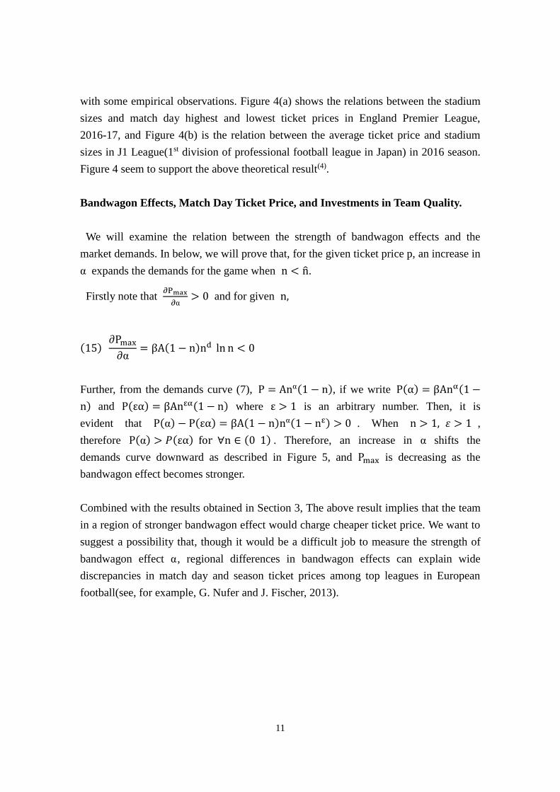
Bandwagon Effects, Match Day Ticket Price, and Investments in Team Quality.

We will examine the relation between the strength of bandwagon effects and the

market demands. In below, we will prove that, for the given ticket price p, an increase in

α expands the demands for the game when n < n̂.

Firstly note that ∂Pmax

∂α> 0 and for given n,

(15) ∂Pmax

∂α= βA(1 − n)nd ln n < 0

Further, from the demands curve (7), P = Anα(1 − n), if we write P(α) = βAnα(1 −

n) and P(εα) = βAnεα(1 − n) where ε > 1 is an arbitrary number. Then, it is

evident that P(α) − P(εα) = βA(1 − n)nα(1 − nε) > 0 . When n > 1, 𝜀 > 1 ,

therefore P(α) > 𝑃(εα) for ∀n ∈ (0 1) . Therefore, an increase in α shifts the

demands curve downward as described in Figure 5, and Pmax is decreasing as the

bandwagon effect becomes stronger.

Combined with the results obtained in Section 3, The above result implies that the team

in a region of stronger bandwagon effect would charge cheaper ticket price. We want to

suggest a possibility that, though it would be a difficult job to measure the strength of

bandwagon effect α, regional differences in bandwagon effects can explain wide

discrepancies in match day and season ticket prices among top leagues in European

football(see, for example, G. Nufer and J. Fischer, 2013).

12

FIGURE 5

Next, we will investigate the relation between the bandwagon effect and monopoly’s

investment to team quality.

When n̅ < n̂, we redefine the profit from the game as

(16) π = Pmax ∙ n̅ − (c + ωq)

= hA(q)n̅ − (c + ωq)

Where h = β (αα

(1+α)1+α) , and q means the total number of talents that the team

possesses, ω is the unit cost of talents, c is the other fixed costs(see, for example, S.

Kesenne, 2007). From above, it follows that,

∂π

∂q= hA′(q)n̅ − ω

∂2π

∂q2 = hA′′(q)n̅ < 0.

13

If we define q∗ by A′(q∗) =ω

hn̅, it follows

(17) ∂q∗

∂ω=

1

A′′hn̅< 0

(18) ∂q∗

∂n̅= −

A′

A′′n̅> 0

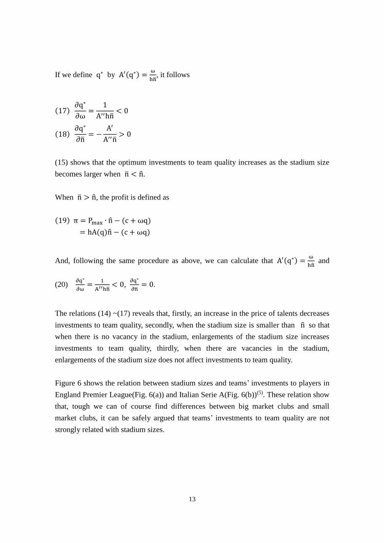
(15) shows that the optimum investments to team quality increases as the stadium size

becomes larger when n̅ < n̂.

When n̅ > n̂, the profit is defined as

(19) π = Pmax ∙ n̂ − (c + ωq)

= hA(q)n̂ − (c + ωq)

And, following the same procedure as above, we can calculate that A′(q∗) =ω

hn̂ and

(20) ∂q∗

∂ω=

1

A′′hn̂< 0,

∂q∗

∂n̅= 0.

The relations (14) ~(17) reveals that, firstly, an increase in the price of talents decreases

investments to team quality, secondly, when the stadium size is smaller than n̂ so that

when there is no vacancy in the stadium, enlargements of the stadium size increases

investments to team quality, thirdly, when there are vacancies in the stadium,

enlargements of the stadium size does not affect investments to team quality.

Figure 6 shows the relation between stadium sizes and teams’ investments to players in

England Premier League(Fig. 6(a)) and Italian Serie A(Fig. 6(b))(5). These relation show

that, tough we can of course find differences between big market clubs and small

market clubs, it can be safely argued that teams’ investments to team quality are not

strongly related with stadium sizes.

14

FIGURE 6(a)

FIGURE 6(b)

Concluding Remarks

Recent years have witnessed a boom of researches exploring the possible relations

between social relations and market demands, and this study can be viewed as one of

these researches. We elaborate Becker’s inferences(1991) that bandwagon effects could

bring an upward sloping demand curves, and examine how bandwagon effects would

affects local monopoly pricing in sports product market. We establish a case wherein

Becker’s inferences are valid and make explicit what has been implicit in Becker’s

arguments. We can derive further implications of the upward demanding curve

combined with local monopoly by specifying the strength of bandwagon effects. We

15

explain the excess demand and supply, often observed in professional team sports

worldwide, as equilibrium phenomena wherein both consumers’ utilities and producer’s

profit are maximized. We provide a view that this seemingly awkward “equilibrium” is

ascribed to bandwagon effects associated with upward demand curves and market

structure of local monopoly.

Upward sloping demand curves would yield several new insights in studies about

competitive balance, revenue sharing, players’ labor markets and other important

research areas of professional team sports markets. We think the model we propose in

this study could be extended and applied in these directions. However, an important

question remains unanswered in this study, that is, the very basic question how we can

measure the bandwagon effect from the empirical data. We think this measurement

problem is related with our understanding or interpretation of social and psychological

forces underlying bandwagon-like behaviors. For example, it might be that bandwagon

effects are the results of identity confirming behaviors of consumers. If identity

confirming behavior enhances consumers’ utilities and identity confirming is made by

mimicking the behaviors of others(of same social identity group) as postulated by

Akerlof and Kranton(2000), then bandwagon effects in this study could be explained as

behaviors of regional identity confirmation. Under this situation, the strength of

bandwagon effects would be partly determined by the historical process under which

local professional sports club has been related to local identity of the region.

16

Footnotes.

(1) Becker’s postulation is analyzed in a game theory framework by Karni and

Levin(1994), for which Plott and Smith(1999) indicate behavioral inconsistencies of

basic assumptions they adopted.

(2) The demand curve in Figure 2 shows the relation between the market demand and

the reservation price of the marginal attendant, which is somewhat different from the

ordinary demand curves representing the sum of individual demands for given

prices. We think this raises some confusion among the researchers. For example,

Gisser et.al.(2009) wrote, “ if the zigzagged curve that Becker(1991) labeled “d”

shown in Figure 1 is not really a demand curve then the question becomes: What is

it?”.

(3) In this study, we explain the excess demand and excess supply as phenomena

observed under “market equilibrium” – equilibrium in the sense that producer’s

profit and consumers’ utilities are maximized.

(4) The data for England Premier League is from BBC SPORT football(2016) and the

data for J1 League is from Football GEIST(2016).

(5) The data for Italian Serie A is from “Serie A Transfer and Wage Budgets”,

REALSPORT(Nov. 11, 2016) and the for stadium sizes are from BBC SPORT

football(2016) and “List of English Football Stadiums by Capacity(Wikipedia)”.

17

References.

Akerlof, G. A. and Kranton, R.E.(2000). Economics and Identity. Quarterly Journal of

Economics, 115, 715-753.

Becker, Gary(1991). A Note on Restaurant Pricing and Other Examples of Social

Influences on Price. Journal of Political Economy, 99, 1109-1116.

Gisser, M., J. McClure, G. Okten, and G. Santoni(2009). Some Anomalies Arising from

Bandwagons that Impart Upward Sloping Segments to Market Demand. Economics

Journals Watch, 6. 21-33.

Karni, Edi and Dan Levin(1994). Social Attitudes and Strategic Equlibrium:A

Restaurant Pricing Game, Journal of Political Economy, 102, 822-840.

Kesenne, Stefan(2007). The Economic Theory of Professional Team Sports, Edward

Elgar Publishing

Leibenstein, H(1950). Bandwagon, Snob and Veblen Effects in the Theory of

Consumers’ Demand, Quarterly Journal of Economics, 64, 183-207.

Nuffer Gerd and Jan Fischer(2013). Ticket Pricing in European Football- Analysis and

Implications. Sports and Arts, 1. 49-60.

Pepall, Lynne and Joseph Reiff(2016). The “Vebeln” Effect, Targeted Advertising and

Consumer Welfare. Economics Department Working Paper, Tufts University.

Plott, Charles R. and Jared Smith(1999). Instability of Equilibria in Experimental

Markets: Upward-sloping Demand Externalities. Southern Economic Journal,

65.405-426.