Embed Size (px)
Citation preview

GRAPHICAL MODELS WITH STRUCTUREDFACTORS, NEURAL FACTORS, ANDAPPROXIMATION-AWARE TRAINING
byMatthew R. Gormley
A dissertation submitted to Johns Hopkins University in conformitywith the requirements for the degree of Doctor of Philosophy
Baltimore, MDOctober 2015
c⃝2015 Matthew R. GormleyAll Rights Reserved

Abstract
This thesis broadens the space of rich yet practical models for structured prediction. We
introduce a general framework for modeling with four ingredients: (1) latent variables,
(2) structural constraints, (3) learned (neural) feature representations of the inputs, and
(4) training that takes the approximations made during inference into account. The thesis
builds up to this framework through an empirical study of three NLP tasks: semantic role
labeling, relation extraction, and dependency parsing—obtaining state-of-the-art results on
the former two. We apply the resulting graphical models with structured and neural fac-
tors, and approximation-aware learning to jointly model part-of-speech tags, a syntactic
dependency parse, and semantic roles in a low-resource setting where the syntax is unob-
served. We present an alternative view of these models as neural networks with a topology
inspired by inference on graphical models that encode our intuitions about the data.
Keywords: Machine learning, natural language processing, structured prediction, graph-
ical models, approximate inference, semantic role labeling, relation extraction, dependency
parsing.
Thesis Committee: (†advisors)
†Jason Eisner (Professor, Computer Science, Johns Hopkins University)
†Mark Dredze (Assistant Research Professor, Computer Science, Johns Hopkins University)
Benjamin Van Durme (Assistant Research Professor, Computer Science, Johns Hopkins University)
Slav Petrov (Staff Research Scientist, Google)
ii

Acknowledgements
First, I thank my co-advisors, Jason Eisner and Mark Dredze, who always managed to
align their advice exactly when it mattered and challenge me through their opposition on
everything else. Jason exemplified for me how to think like a visionary and to broaden my
sights as a researcher, even as we continually delved deeper into our work. Mark taught me
to take a step back from my research and ambitions. He showed me how to be an empiricist,
a pragmatist, and a scientist. Together, Mark and Jason demonstrated all the best qualities
of advisors, teachers, and mentors. I hope that some of it rubbed off on me.
Thanks to my committee members, Benjamin Van Durme and Slav Petrov, alongside
Jason Eisner and Mark Dredze. Ben frequently took on the role of both publisher and critic
for my work: he advertised the real-world applications of my research and challenged me to
consider the linguistic underpinnings. At every step along the way, Slav’s forward-looking
questions were predictive of the details that would require the most attention.
Many faculty at Johns Hopkins impacted me through teaching, conversations, and men-
toring. In particular, I would like to thank those who made my experience at the Center for
Language and Speech Processing (CLSP) and the Human Language Technology Center of
Excellence (HLTCOE) so rich: Sanjeev Khudanpur, Matt Post, Adam Lopez, Jim Mayfield,
Mary Harper, David Yarowsky, Chris Callison-Burch, and Suchi Saria. Working with other
researchers taught me a lot: thanks to Spence Green, Dan Bikel, Jakob Uszkoreit, Ashish
Venugopal, and Percy Liang. Emails exchanges with Jason Naradowsky, Andre Martins,
Alexander Rush, and Valentin Spitkovsky were key for replicating prior work. Thanks to
iii

David Smith, Zhifei Li, and Veselin Stoyanov, who did work that was so complementary
that we couldn’t resist putting it all together.
The staff at the CLSP, the HLTCOE, and the CS Department made everything a breeze,
from high performance computing to finding a classroom at the last minute—special thanks
to Max Thomas and Craig Harman because good code drives research.
My fellow students and postdocs made this thesis possible. My collaborations with Mo
Yu and Meg Mitchell deserve particular note. Mo taught me how to use every trick in the
book, and then invent three more. Meg put up with and encouraged my incessant over-
engineering that eventually led to Pacaya. To my lab mates, I can’t say thank you enough:
Nick Andrews, Tim Vieira, Frank Ferraro, Travis Wolfe, Jason Smith, Adam Teichart,
Dingquan Wang, Veselin Stoyanov, Sharon Li, Justin Snyder, Rebecca Knowles, Nathanial
Wes Filardo, Michael Paul, Nanyun Peng, Markus Dreyer, Carolina Parada, Ann Irvine,
Courtney Napoles, Darcey Riley, Ryan Cotterell, Tongfei Chen, Xuchen Yao, Pushpendre
Rastogi, Brian Kjersten, and Ehsan Variani.
I am indebted to my friends in Baltimore. Thanks to: Andrew for listening to my
research ramblings over lunch; Alan and Nick for much needed sports for the sake of rest;
the Bettles, the Kuks, and the Lofti for mealshare and more; everyone who babysat; Merv
and the New Song Men’s Bible Study for giving me perspective.
Thanks to nutat and nunan for teaching me to seek first Jesus in all that I do. Thanks to
my anabixel, baluk, and ch’utin mial for introducing me to K’iche’ and giving me a second
home in Guatemala. Esther, thanks—you were all the motivation I needed to finish.
To my wife, Candice Gormley: you deserve the most thanks of all. You got us through
every success and failure of my Ph.D. Most importantly, you showed me how to act justly,
love mercy, and walk humbly with our God.
iv

Contents
Abstract ii
Acknowledgements iii
Contents x
List of Tables xii
List of Figures xiv
1 Introduction 1
1.1 Motivation and Prior Work . . . . . . . . . . . . . . . . . . . . . . . . . . 2
1.1.1 Why do we want to build rich (joint) models? . . . . . . . . . . . . 2
1.1.2 Inference with Structural Constraints . . . . . . . . . . . . . . . . 4
1.1.3 Learning under approximations . . . . . . . . . . . . . . . . . . . 5
1.1.4 What about Neural Networks? . . . . . . . . . . . . . . . . . . . . 6
1.2 Proposed Solution . . . . . . . . . . . . . . . . . . . . . . . . . . . . . . . 7
1.3 Contributions and Thesis Statement . . . . . . . . . . . . . . . . . . . . . 8
1.4 Organization of This Dissertation . . . . . . . . . . . . . . . . . . . . . . . 11
1.5 Preface and Other Publications . . . . . . . . . . . . . . . . . . . . . . . . 12
2 Background 14
2.1 Preliminaries . . . . . . . . . . . . . . . . . . . . . . . . . . . . . . . . . 14
v

CONTENTS
2.1.1 A Simple Recipe for Machine Learning . . . . . . . . . . . . . . . 14
2.2 Neural Networks and Backpropagation . . . . . . . . . . . . . . . . . . . . 16
2.2.1 Topologies . . . . . . . . . . . . . . . . . . . . . . . . . . . . . . 16
2.2.2 Backpropagation . . . . . . . . . . . . . . . . . . . . . . . . . . . 18
2.2.3 Numerical Differentiation . . . . . . . . . . . . . . . . . . . . . . 20
2.3 Graphical Models . . . . . . . . . . . . . . . . . . . . . . . . . . . . . . . 21
2.3.1 Factor Graphs . . . . . . . . . . . . . . . . . . . . . . . . . . . . . 21
2.3.2 Minimum Bayes Risk Decoding . . . . . . . . . . . . . . . . . . . 23
2.3.3 Approximate Inference . . . . . . . . . . . . . . . . . . . . . . . . 24
2.3.3.1 Belief Propagation . . . . . . . . . . . . . . . . . . . . . 25
2.3.3.2 Loopy Belief Propagation . . . . . . . . . . . . . . . . . 27
2.3.3.3 Bethe Free Energy . . . . . . . . . . . . . . . . . . . . . 28
2.3.3.4 Structured Belief Propagation . . . . . . . . . . . . . . . 29
2.3.4 Training Objectives . . . . . . . . . . . . . . . . . . . . . . . . . . 32
2.3.4.1 Conditional Log-likelihood . . . . . . . . . . . . . . . . 32
2.3.4.2 CLL with Latent Variables . . . . . . . . . . . . . . . . 34
2.3.4.3 Empirical Risk Minimization . . . . . . . . . . . . . . . 35
2.3.4.4 Empirical Risk Minimization Under Approximations . . 36
2.4 Continuous Optimization . . . . . . . . . . . . . . . . . . . . . . . . . . . 36
2.4.1 Online Learning and Regularized Regret . . . . . . . . . . . . . . . 38
2.4.2 Online Learning Algorithms . . . . . . . . . . . . . . . . . . . . . 39
2.4.2.1 Stochastic Gradient Descent . . . . . . . . . . . . . . . . 40
2.4.2.2 Mirror Descent . . . . . . . . . . . . . . . . . . . . . . . 40
2.4.2.3 Composite Objective Mirror Descent . . . . . . . . . . . 41
2.4.2.4 AdaGrad . . . . . . . . . . . . . . . . . . . . . . . . . . 41
2.4.2.5 Parallelization over Mini-batches . . . . . . . . . . . . . 43
vi

CONTENTS
3 Latent Variables and Structured Factors 45
3.1 Introduction . . . . . . . . . . . . . . . . . . . . . . . . . . . . . . . . . . 46
3.2 Approaches . . . . . . . . . . . . . . . . . . . . . . . . . . . . . . . . . . 49
3.2.1 Pipeline Model with Unsupervised Syntax . . . . . . . . . . . . . . 49
3.2.1.1 Brown Clusters . . . . . . . . . . . . . . . . . . . . . . 50
3.2.1.2 Unsupervised Grammar Induction . . . . . . . . . . . . 50
3.2.1.3 Semantic Dependency Model . . . . . . . . . . . . . . . 51
3.2.2 Pipeline Model with Distantly-Supervised Syntax . . . . . . . . . . 52
3.2.2.1 Constrained Grammar Induction . . . . . . . . . . . . . 54
3.2.3 Joint Syntactic and Semantic Parsing Model . . . . . . . . . . . . . 54
3.2.4 Pipeline Model with Supervised Syntax (Skyline) . . . . . . . . . . 56
3.2.5 Features for CRF Models . . . . . . . . . . . . . . . . . . . . . . . 57
3.2.5.1 Template Creation from Properties of Ordered Positions . 57
3.2.5.2 Additional Features . . . . . . . . . . . . . . . . . . . . 62
3.2.6 Feature Selection . . . . . . . . . . . . . . . . . . . . . . . . . . . 62
3.3 Related Work . . . . . . . . . . . . . . . . . . . . . . . . . . . . . . . . . 63
3.4 Experimental Setup . . . . . . . . . . . . . . . . . . . . . . . . . . . . . . 66
3.4.1 Data . . . . . . . . . . . . . . . . . . . . . . . . . . . . . . . . . . 66
3.4.2 Feature Template Sets . . . . . . . . . . . . . . . . . . . . . . . . 67
3.5 Results . . . . . . . . . . . . . . . . . . . . . . . . . . . . . . . . . . . . . 68
3.5.1 CoNLL-2009: High-resource SRL . . . . . . . . . . . . . . . . . . 68
3.5.2 CoNLL-2009: Low-Resource SRL . . . . . . . . . . . . . . . . . . 70
3.5.3 CoNLL-2008, -2005 without a Treebank . . . . . . . . . . . . . . 73
3.5.4 Analysis of Grammar Induction . . . . . . . . . . . . . . . . . . . 75
3.6 Summary . . . . . . . . . . . . . . . . . . . . . . . . . . . . . . . . . . . 76
4 Neural and Log-linear Factors 78
4.1 Introduction . . . . . . . . . . . . . . . . . . . . . . . . . . . . . . . . . . 79
vii

CONTENTS
4.2 Relation Extraction . . . . . . . . . . . . . . . . . . . . . . . . . . . . . . 82
4.3 Background: Compositional Embedding Model . . . . . . . . . . . . . . . 84
4.3.1 Combining Features with Embeddings . . . . . . . . . . . . . . . . 84
4.3.2 The Log-Bilinear Model . . . . . . . . . . . . . . . . . . . . . . . 86
4.3.3 Discussion of the Compositional Model . . . . . . . . . . . . . . . 87
4.4 A Log-linear Model . . . . . . . . . . . . . . . . . . . . . . . . . . . . . . 88
4.5 Hybrid Model . . . . . . . . . . . . . . . . . . . . . . . . . . . . . . . . . 89
4.6 Main Experiments . . . . . . . . . . . . . . . . . . . . . . . . . . . . . . . 91
4.6.1 Experimental Settings . . . . . . . . . . . . . . . . . . . . . . . . 91
4.6.2 Results . . . . . . . . . . . . . . . . . . . . . . . . . . . . . . . . 95
4.7 Additional ACE 2005 Experiments . . . . . . . . . . . . . . . . . . . . . . 99
4.7.1 Experimental Settings . . . . . . . . . . . . . . . . . . . . . . . . 99
4.7.2 Results . . . . . . . . . . . . . . . . . . . . . . . . . . . . . . . . 100
4.8 Related Work . . . . . . . . . . . . . . . . . . . . . . . . . . . . . . . . . 101
4.9 Summary . . . . . . . . . . . . . . . . . . . . . . . . . . . . . . . . . . . 103
5 Approximation-aware Learning for Structured Belief Propagation 105
5.1 Introduction . . . . . . . . . . . . . . . . . . . . . . . . . . . . . . . . . . 106
5.2 Dependency Parsing by Belief Propagation . . . . . . . . . . . . . . . . . 108
5.3 Approximation-aware Learning . . . . . . . . . . . . . . . . . . . . . . . . 112
5.4 Differentiable Objective Functions . . . . . . . . . . . . . . . . . . . . . . 116
5.4.1 Annealed Risk . . . . . . . . . . . . . . . . . . . . . . . . . . . . 116
5.4.2 L2 Distance . . . . . . . . . . . . . . . . . . . . . . . . . . . . . . 117
5.4.3 Layer-wise Training . . . . . . . . . . . . . . . . . . . . . . . . . 118
5.4.4 Bethe Likelihood . . . . . . . . . . . . . . . . . . . . . . . . . . . 118
5.5 Gradients by Backpropagation . . . . . . . . . . . . . . . . . . . . . . . . 118
5.5.1 Backpropagation of Decoder / Loss . . . . . . . . . . . . . . . . . 119
5.5.2 Backpropagation through Structured BP . . . . . . . . . . . . . . . 119
viii

CONTENTS
5.5.3 BP and Backpropagation with PTREE . . . . . . . . . . . . . . . . 120
5.5.4 Backprop of Hypergraph Inside-Outside . . . . . . . . . . . . . . . 122
5.6 Other Learning Settings . . . . . . . . . . . . . . . . . . . . . . . . . . . . 124
5.7 Experiments . . . . . . . . . . . . . . . . . . . . . . . . . . . . . . . . . . 125
5.7.1 Setup . . . . . . . . . . . . . . . . . . . . . . . . . . . . . . . . . 125
5.7.2 Results . . . . . . . . . . . . . . . . . . . . . . . . . . . . . . . . 128
5.8 Discussion . . . . . . . . . . . . . . . . . . . . . . . . . . . . . . . . . . . 131
5.9 Summary . . . . . . . . . . . . . . . . . . . . . . . . . . . . . . . . . . . 133
6 Graphical Models with Structured and Neural Factors and Approximation-
aware Learning 134
6.1 Introduction . . . . . . . . . . . . . . . . . . . . . . . . . . . . . . . . . . 135
6.2 Model . . . . . . . . . . . . . . . . . . . . . . . . . . . . . . . . . . . . . 137
6.3 Inference . . . . . . . . . . . . . . . . . . . . . . . . . . . . . . . . . . . 139
6.4 Decoding . . . . . . . . . . . . . . . . . . . . . . . . . . . . . . . . . . . 141
6.5 Learning . . . . . . . . . . . . . . . . . . . . . . . . . . . . . . . . . . . . 142
6.5.1 Approximation-Unaware Training . . . . . . . . . . . . . . . . . . 142
6.5.2 Approximation-Aware Training . . . . . . . . . . . . . . . . . . . 143
6.6 Experiments . . . . . . . . . . . . . . . . . . . . . . . . . . . . . . . . . . 144
6.6.1 Experimental Setup . . . . . . . . . . . . . . . . . . . . . . . . . . 144
6.6.2 Results . . . . . . . . . . . . . . . . . . . . . . . . . . . . . . . . 146
6.6.3 Error Analysis . . . . . . . . . . . . . . . . . . . . . . . . . . . . 150
6.7 Summary . . . . . . . . . . . . . . . . . . . . . . . . . . . . . . . . . . . 154
7 Conclusions 155
7.1 Summary of the Thesis . . . . . . . . . . . . . . . . . . . . . . . . . . . . 155
7.2 Future Work . . . . . . . . . . . . . . . . . . . . . . . . . . . . . . . . . . 156
7.2.1 Other Structured Factors and Applications . . . . . . . . . . . . . . 156
ix
CONTENTS
7.2.2 Pruning-aware Learning . . . . . . . . . . . . . . . . . . . . . . . 157
7.2.3 Hyperparameters: Optimizing or Avoiding . . . . . . . . . . . . . 158
7.2.4 Multi-task Learning for Domain Adaptation . . . . . . . . . . . . . 159
A Pacaya: A General Toolkit for Graphical Models, Hypergraphs, and Neural
Networks 161
A.1 Code Layout . . . . . . . . . . . . . . . . . . . . . . . . . . . . . . . . . . 161
A.2 Feature Sets from Prior Work . . . . . . . . . . . . . . . . . . . . . . . . . 163
A.3 Design . . . . . . . . . . . . . . . . . . . . . . . . . . . . . . . . . . . . . 164
A.3.1 Differences from Existing Libraries . . . . . . . . . . . . . . . . . 164
A.3.2 Numerical Stability and Efficient Semirings in Java . . . . . . . . . 165
A.3.3 Comments on Engineering the System . . . . . . . . . . . . . . . . 166
A.3.3.1 Experiment 1: Inside-Outside Algorithm . . . . . . . . . 167
A.3.3.2 Experiment 2: Parallel Belief Propagation . . . . . . . . 169
B Bethe Likelihood 171
Bibliography 197
Vita 198
x
List of Tables
2.1 Brief Summary of Notation . . . . . . . . . . . . . . . . . . . . . . . . . . 15
3.1 Feature templates for semantic role labeling . . . . . . . . . . . . . . . . . 58
3.2 Feature templates selected by information gain for SRL. . . . . . . . . . . 64
3.3 Test F1 of supervised SRL and sense disambiguation with gold (oracle)
syntax averaged over the CoNLL-2009 languages. See Table 3.6(a) for
per-language results. . . . . . . . . . . . . . . . . . . . . . . . . . . . . . 69
3.4 Test F1 of supervised SRL and sense disambiguation with supervised syn-
tax, averaged over CoNLL-2009 languages. See Table 3.6(b) for per-language
results. . . . . . . . . . . . . . . . . . . . . . . . . . . . . . . . . . . . . . 70
3.5 Test F1 of supervised SRL and sense disambiguation with no supervision
for syntax, averaged over CoNLL-2009 languages. See Table 3.6(c) for
per-language results. . . . . . . . . . . . . . . . . . . . . . . . . . . . . . 71
3.6 Performance of joint and pipelined models for semantic role labeling in
high-resource and low-resource settings on CoNLL-2009. . . . . . . . . . . 72
3.7 Performance of semantic role labelers with descreasing annotated resources. 73
3.8 Performance of semantic role labelers in matched and mismatched train/test
settings on CoNLL 2005/2008. . . . . . . . . . . . . . . . . . . . . . . . . 74
3.9 Performance of grammar induction on CoNLL-2009. . . . . . . . . . . . . 76
3.10 Performance of grammar induction on the Penn Treebank. . . . . . . . . . 77
xi

LIST OF TABLES
4.1 Example relations from ACE 2005. . . . . . . . . . . . . . . . . . . . . . . 79
4.2 Feature sets used in FCM. . . . . . . . . . . . . . . . . . . . . . . . . . . . 92
4.3 Named entity tags for ACE 2005 and SemEval 2010. . . . . . . . . . . . . 95
4.4 Performance of relation extractors on ACE 2005 out-of-domain test sets. . . 96
4.5 Performance of relation extractors on SemEval 2010 Task 8. . . . . . . . . 98
4.6 Performance of relation extractors on ACE 2005 out-of-domain test sets for
the low-resource setting. . . . . . . . . . . . . . . . . . . . . . . . . . . . 101
5.1 Belief propagation unrolled through time. . . . . . . . . . . . . . . . . . . 121
5.2 Impact of exact vs. approximate inference on a dependency parser. . . . . . 130
5.3 Full performance results of dependency parser on 19 languages from CoNLL-
2006/2007. . . . . . . . . . . . . . . . . . . . . . . . . . . . . . . . . . . 132
6.1 Additive experiment for five languages from CoNLL-2009. . . . . . . . . . 147
6.2 Performance of approximation-aware learning on semantic role labeling. . . 148
6.3 SRL performance on four models for error analysis. . . . . . . . . . . . . . 151
6.4 Performance of SRL across role labels. . . . . . . . . . . . . . . . . . . . . 154
7.1 Example sentences from newswire and Twitter domains. . . . . . . . . . . 158
A.1 Speed comparison of inside algorithm implementations . . . . . . . . . . . 168
A.2 Speed comparison of BP implementations . . . . . . . . . . . . . . . . . . 169
xii

List of Figures
2.1 Feed-forward topology of a 2-layer neural network. . . . . . . . . . . . . . 17
2.2 Example factor graphs. . . . . . . . . . . . . . . . . . . . . . . . . . . . . 22
2.3 Feed-forward topology of inference, decoding, and loss according to ERMA. 37
3.1 Diagram of the pipeline approach to semantic role labeling. . . . . . . . . . 49
3.2 Example semantic roles for sentence and the corresponding variable as-
signment of the factor graph for the semantic dependency model. . . . . . . 52
3.3 Example of a pruned parse chart for constrained grammar induction. . . . . 53
3.4 Factor graph for the joint syntactic/semantic dependency parsing model. . . 55
3.5 Performance of semantic role labelers with varying numbers of of training
examples. . . . . . . . . . . . . . . . . . . . . . . . . . . . . . . . . . . . 74
4.1 Example construction of FCM substructure embeddings. . . . . . . . . . . . 84
4.2 Factor graph of the hybrid log-linear and neural network model. . . . . . . 90
5.1 Factor graph for dependency parsing model. . . . . . . . . . . . . . . . . . 108
5.2 Feed-forward topology of inference, decoding, and loss. . . . . . . . . . . 115
5.3 Speed/accuracy tradeoff of the dependency parser on the Penn Treebank. . . 127
5.4 Performance of four different dependency parsers with and without approximation-
aware training on the Penn Treebank. . . . . . . . . . . . . . . . . . . . . . 128
5.5 Performance improvement given by using approximation-aware training on
19 languages from CoNLL-2006/2007. . . . . . . . . . . . . . . . . . . . . 131
xiii

LIST OF FIGURES
6.1 Factor graph for joint semantic and syntactic dependency parsing and syn-
tactic tagging. . . . . . . . . . . . . . . . . . . . . . . . . . . . . . . . . . 140
6.2 Performance of low-resource SRL on English CoNLL-2009. . . . . . . . . 149
6.3 Performance of SRL for predicate-argument distance. . . . . . . . . . . . . 152
6.4 Performance of SRL across nominal and verbal predicates. . . . . . . . . . 153
xiv

Chapter 1
Introduction
A common tension in machine learning is the tradeoff between designing models which
are practical to use and those which capture our intuitions about the underlying data. This
tension is particularly salient in natural language processing (NLP). To be useful, an NLP
tool must (often) process text faster than it can be spoken or written. Linguistics pro-
vides explanations of generative processes which govern that data. Yet designing models
that mirror these linguistic processes would quickly lead to intractability for inference and
learning. This is not just a grievance for NLP researchers: for many machine learning prob-
lems there is real-world knowledge of the data that could inform model design but practical
considerations rein in our ambitions. A key goal of machine learning is to enable this use
of richer models.
This thesis broadens the space of rich yet practical probabilistic models for structured
prediction. We introduce a general framework for modeling with four ingredients: (1) la-
tent variables, (2) structural constraints, (3) learned (neural) feature representations of the
inputs, and (4) training that takes the approximations made during inference into account.
The thesis builds up to this framework through an empirical study of three NLP tasks:
semantic role labeling, relation extraction, and dependency parsing—obtaining state-of-
the-art results on the former two. We apply the resulting graphical models with structured
1

1.1. MOTIVATION AND PRIOR WORK
and neural factors, and approximation-aware learning to jointly model syntactic depen-
dency parsing and semantic role labeling in a low-resource setting where the syntax is
unobserved. We also present an alternative view of these models as neural networks with
a topology inspired by inference on graphical models that encode our intuitions about the
data.
In order to situate our contributions in the literature, we next discuss related approaches
and highlight prior work that acts as critical building blocks for this thesis (Section 1.1).
After stating our proposed solution (Section 1.2), we provide a succinct statement of the
contributions (Section 1.3) and organization (Section 1.4) of this dissertation.
1.1 Motivation and Prior Work
In this section, we discuss the reasons behind the design of the modeling framework pre-
sented in this thesis. By considering a simple example, that is representative of many ap-
plication areas in machine learning, we hope to elicit the need for latent variable modeling,
structured prediction, learning with inexact inference, and neural networks. Our focus here
is on the solved and open problems in these areas, leaving detailed discussions of related
work to later chapters.
1.1.1 Why do we want to build rich (joint) models?
One of the major limitations to machine learning is data collection. It is expensive to
obtain and just when we think we have enough, a new domain for our task—or a new
task altogether—comes up. Without annotated data, one might naturally gravitate to un-
supervised learning. For example, in NLP, syntactic treebanks are difficult to build, so re-
searchers (including this one) have looked to grammar induction (the unsupervised learning
of syntactic parsers) for a solution (Smith (2006) and Spitkovsky (2013) represent observ-
able progress). Yet fully unsupervised learning has two problems:
2

1.1. MOTIVATION AND PRIOR WORK
1. It’s not tuned for any downstream task. Thus, the resulting predictions may or may
not be useful.
2. Usually, if you have even a very small number of training examples, you can outper-
form the best fully unsupervised system easily. (Often even a few handwritten rules
can do better, for the case of grammar induction (Haghighi and Klein, 2006; Naseem
et al., 2010; Søgaard, 2012).)
So, the question remains: how can we design high-performing models that are less
reliant on hand annotated data? The solution proposed by this thesis has two related facets:
First, do not throw away the idea of learning latent structure (a la grammar induction);
instead build it into a larger joint model. Second, do not discard data if you have it; build a
joint model that can use whatever informative data you have. Let’s take an example.
Example: Suppose you want to do relation extraction on weblogs. You al-
ready have data for (a) relations on weblogs, (b) syntax on newswire, and (c)
named entities on broadcast news. Certainly it would be foolish to throw away
datasets (b) and (c) altogether. The usual NLP approach is to train a pipeline
of systems: (a) relation extractor, (b) parser, and (c) named entity recognizer,
with features of the latter two providing information to the relation extractor.
However, we don’t actually believe that a parser trained on newswire knows
exactly what the trees on weblogs look like. But without a joint model of rela-
tions, parses, and named entities there’s no opportunity for feedback between
the components of the pipeline. A joint model recognizes that there are latent
trees and named entities on the weblogs; and we should use the equivalent an-
notations on newswire and broadcast news to influence what we believe them
to be.
Should we use this fancy rich model when we have lots of supervision? The jury is still
out on that one; but there are plenty of examples that suggest the gains from joint modeling
3

1.1. MOTIVATION AND PRIOR WORK
may be minimal if you have lots of data (cf. Gesmundo et al. (2009), Hajic et al. (2009),
and Lluıs et al. (2013)). The key tradeoff is that incorporating increasingly global features
leads to better models of the data, but it also makes inference more challenging. However,
whether we should use a joint model when supervision is scarce is an open question, and
this thesis begins to address it.
1.1.2 Inference with Structural Constraints
As alluded to above, increasingly rich models often lead to more expensive inference. If
exact inference is too hard, can’t we just rely on approximate inference? That depends
on what sort of models we actually want to build, and just how fast inference needs to
be. Going back to our example, if we assume that we’ll be modeling syntax or semantics
as latent, we’ll need to encode some real-world knowledge about how they behave in the
form of declarative constraints. In the language of graphical models, these constraints
correspond to structured factors that express an opinion about many variables at once. The
basic variants of inference for graphical models don’t know how to account for these sorts
of factors. But there are variants that do.
Graphical models provide a concise way of describing a probability distribution over
a structured output space described by a set of variables. Recent advances in approximate
inference have enabled us to consider declarative constraints over the variables. For MAP
inference (finding the variable assignment with maximum score), the proposed methods use
loopy belief propagation (Duchi et al., 2006), integer linear programming (ILP) (Riedel and
Clarke, 2006; Martins et al., 2009), dual decomposition (Koo et al., 2010), or the alternating
directions methods of multipliers (Martins et al., 2011b). For marginal inference (summing
over variable assignments), loopy belief propagation has been employed (Smith and Eisner,
2008). Common to all but the ILP approaches is the embedding of dynamic programming
algorithms (e.g. bipartite matching, forward-backward, inside-outside) within a broader
coordinating framework. Even the ILP algorithms reflect the structure of the dynamic
4

1.1. MOTIVATION AND PRIOR WORK
programming algorithms.
At this point, we must make a decision about what sort of inference we want to do:
• Maximization over the latent variables (MAP inference) sounds good if you believe
that your model will have high confidence and little uncertainty about the values of
those variables. But this directly contradicts the original purpose for which we set
out to use the joint model: we want it to capture the aspects of the data that we’re
uncertain about (because we didn’t have enough data to train a confident model in
the first place).
• Marginalization fits the bill for our setting: we are unsure about a particular assign-
ment to the variables, so each variable can sum out the uncertainty of the others. In
this way, we can quantify our uncertainty about each part of the model, and allow
confidence to propagate through different parts of the model. Choosing structured
belief propagation (BP) (Smith and Eisner, 2008) will ensure we can do so efficiently.
Having chosen marginal inference, we turn to learning.
1.1.3 Learning under approximations
This seems like a promising direction, but there’s one big problem: all of the traditional
learning algorithms assume that inference is exact. The richer we make our model, the
less easy exact inference will be. In practice, we often use approximate inference in place
of exact inference and find the traditional learning algorithms to be effective. However,
the gradients in this setting only approximate and we no longer have guarantees about the
resulting learned model. Not to worry: there are some (lesser used) learning algorithms
that solve exactly this problem.
• For approximate MAP inference there exists a generalization of Collins (2002)’s
structured perceptron to inexact search (e.g. greedy or beam-search algorithms) (Huang
et al., 2012) and its extension to hypergraphs/cube-pruning (Zhang et al., 2013).
5

1.1. MOTIVATION AND PRIOR WORK
• For marginal inference by belief propagation, there have been several approaches that
compute the true gradient of an approximate model either by perturbation (Domke,
2010) or automatic-differentiation (Stoyanov et al., 2011; Domke, 2011).
At first glance, it appears as though we have all the ingredients we need: a rich model that
benefits from the data we have, efficient approximate marginal inference, and learning that
can handle inexact inference. Unfortunately, none of the existing approximation-aware
learning algorithms work with dual decomposition (Koo et al., 2010) or structured BP
(Smith and Eisner, 2008). (Recall that beam search, like dual decomposition, would lose
us the ability to marginalize.) So we’ll have to invent our own. In doing so, we will answer
the question of how one does learning with an approximate marginal inference algorithm
that relies on embedded dynamic programming algorithms.
1.1.4 What about Neural Networks?
If you’ve been following recent trends in machine learning, you might wonder why we’re
considering graphical models at all. During the current re-resurgence of neural networks,
they seem to work very well on a wide variety of applications. As it turns out, we’ll be able
to use neural networks in our framework as well. They will be just another type of factor
in our graphical models. If this hybrid approach to graphical models and neural networks
sounds familiar, that’s because it’s been around for quite a while.
The earliest examples emphasized hybrids of hidden Markov models (HMM) and neu-
ral networks (Bengio et al., 1990; Bengio et al., 1992; Haffner, 1993; Bengio and Frasconi,
1995; Bengio et al., 1995; Bourlard et al., 1995)—recent work has emphasized their com-
bination with energy-based models (Ning et al., 2005; Tompson et al., 2014) and with
probabilistic language models (Morin and Bengio, 2005). Recent work has also explored
the idea of neural factors within graphical models (Do and Artieres, 2010; Srikumar and
Manning, 2014). Notably absent from this line of work are the declarative structural con-
straints mentioned above.
6

1.2. PROPOSED SOLUTION
Neural networks have become very popular in NLP, but are often catered to a single
task. To consider a specific example: the use of neural networks for syntactic parsing has
grown increasingly prominent (Collobert, 2011; Socher et al., 2013a; Vinyals et al., 2015;
Dyer et al., 2015). These models provide a salient example of the use of learned features for
structured prediction, particularly in those cases where the neural network feeds forward
into a standard parsing architecture (Chen and Manning, 2014; Durrett and Klein, 2015;
Pei et al., 2015; Weiss et al., 2015). However, their applicability to the broader space
of structured prediction problems—beyond parsing—is limited. Again returning to our
example, we are interested, by contrast, in modeling multiple linguistic strata jointly.
1.2 Proposed Solution
The far-reaching goal of this thesis is to better enable joint modeling of multi-faceted
datasets with disjointed annotation of corpora. Our canonical example comes from NLP
where we have many linguistic annotations (part-of-speech tags, syntactic parses, semantic
roles, relations, etc.) spread across a variety of different corpora, but rarely all on the same
sentences. A rich joint model of such seemingly disparate data sources would capture all
the linguistic strata at once, taking our uncertainty in account over those not observed at
training time. Thus we require the following:
1. Model representation that supports latent variables and declarative constraints
2. Efficient (assuredly approximate) inference
3. Learning that accounts for the approximations
4. Effective features (optionally learned) that capture the data
Our proposed solution to these problems finds its basis in several key ideas from prior
work. Most notably: (1) factor graphs (Frey et al., 1997; Kschischang et al., 2001) to
represent our model with latent variables and declarative constraints (Naradowsky et al.,
7

1.3. CONTRIBUTIONS AND THESIS STATEMENT
2012a), (3) structured belief propagation (BP) (Smith and Eisner, 2008) for approximate
inference, (4) empirical risk minimization (ERMA) (Stoyanov et al., 2011) and truncated
message passing (Domke, 2011) for learning, and (5) either handcrafted or learned (neural
network-based) features (Bengio et al., 1990). While each of these addresses one or more
of our desiderata above, none of them fully satisfy our requirements. Yet, our framework,
which builds on their combination, does exactly that.
In our framework, our model is defined by a factor graph. Factors express local or
global opinions over subsets of the variables. These opinions can be soft, taking the form
of a log-linear model for example, or can be hard, taking the form of a declarative con-
straint. The factor graph may contain cycles causing exact inference to be intractable in the
general case. Accordingly, we perform approximate marginal inference by structured be-
lief propagation, optionally embedding dynamic programming algorithms inside to handle
the declarative constraint factors or otherwise unwieldy factors. We learn by maximizing
an objective that is computed directly as a function of the marginals output by inference.
The gradient is computed by backpropagation such that the approximations of our entire
system may be taken into account.
The icing on the cake is that neural networks can be easily dropped into this framework
as another type of factor. Notice that inference changes very little with a neural network
as a factor: we simply “feed forward” the inputs through the network to get the scores of
the factor. The neural network acts as an alternative differentiable scoring function for the
factors, replacing the usual log-linear function. Learning is still done by backpropagation,
where we conveniently already know how to backprop through the neural factor.
1.3 Contributions and Thesis Statement
Experimental:
1. We empirically study the merits of latent-variable modeling in pipelined vs.
8

1.3. CONTRIBUTIONS AND THESIS STATEMENT
joint training. Prior work has introduced standalone methods for grammar induc-
tion and methods of jointly inferring a latent grammar with a downstream task. We
fill a gap in the literature by comparing these two approaches empirically. We further
present a new application of unsupervised grammar induction: low-resource seman-
tic role labeling. distantly-supervised, and joint training settings.
2. We provide additional evidence that hand-crafted and learned features are com-
plementary. For the task of relation extraction, we obtain state-of-the-art results
using this combination—further suggesting that both tactics (learning vs. designing
features) have merits.
Modeling:
3. We introduce a new variety of hybrid graphical models and neural networks.
The novel combination of ingredients we propose includes latent variables, structured
factors, and neural factors. When inference is exact, our class of models specifies a
valid probability distribution over the output space. When inference is approximate,
the class of models can be viewed as a form of deep neural network inspired by the
inference algorithms (see Learning below).
4. We present new models for grammar induction, semantic role labeling, relation
extraction, and syntactic dependency parsing. The models we develop include
various combinations of the ingredients mentioned above.
Inference:
5. We unify three forms of inference: loopy belief propagation for graphical mod-
els, dynamic programming in hypergraphs, and feed-forward computation in neural
networks. Taken together, we can view all three as the feed-forward computation of
a very deep neural network whose topology is given by a particular choice of ap-
proximate probabilistic inference algorithm. Alternatively, we can understand this
9
1.3. CONTRIBUTIONS AND THESIS STATEMENT
as a very simple extension of traditional approximate inference in graphical mod-
els with potential functions specified as declarative constraints, neural networks, and
traditional exponential family functions.
Learning:
6. We propose approximation-aware training for structured belief propagation
with neural factors. Treating our favorite algorithms as computational circuits (aka.
deep networks) and running automatic differentiation (aka. backpropagation) to do
end-to-end training is certainly an idea that’s been around for a while (e.g. Bengio
et al. (1995)). We apply this idea to models with structured and neural factors and
demonstrate its effectiveness over a strong baseline. This extends prior work which
focused on message passing algorithms for approximate inference with standard fac-
tors (Stoyanov et al., 2011; Domke, 2011).
7. We introduce new training objectives for graphical models motivated by neural
networks. Viewing graphical models as a form of deep neural network naturally
leads us to explore objective functions that (albeit common to neural networks) are
novel to training of graphical models.
Thesis Statement We claim that the accuracy of graphical models can be improved by
incorporating methods that are typically reserved for approaches considered to be distinct.
First, we aim to validate that joint modeling with latent variables is effective at improving
accuracy over standalone grammar induction. Second, we claim that incorporating neural
networks alongside handcrafted features provides gains for graphical models. Third, taking
the approximations of an entire system into account provides additional gains and can be
done even with factors of many variables when they exhibit some special structure. Fi-
nally, we argue that the sum of these parts will provide new effective models for structured
prediction.
10

1.4. ORGANIZATION OF THIS DISSERTATION
1.4 Organization of This Dissertation
This primary contributions of this thesis are four content chapters: Chapters 3, 4, and
5 each explore a single extension to traditional graphical models (each with a different
natural language application) and Chapter 6 combines these three extensions to show their
complementarity.
• Chapter 2: Background. The first section places two distinct modeling approaches
side-by-side: graphical models and neural networks. The similarities between the
two are highlighted and a common notation is established. We briefly introduce the
types of natural language structures that will form the basis of our application areas
(deferring further application details to later chapters). Using the language of hyper-
graphs, we review dynamic programming algorithms catered to these structures. We
emphasize the material that is essential for understanding the subsequent chapters
and for differentiating our contributions.
• Chapter 3: Latent Variables and Structured Factors (Semantic Role Labeling). This
chapter motivates our approach by providing an empirical contrast of three approaches
to grammar induction with the aim of improving semantic role labeling. Experiments
are presented on 6 languages.
• Chapter 4: Neural and Log-linear Factors (Relation Extraction). We present new
approaches for relation extraction that combine the benefits of traditional feature-
based log-linear models and neural networks (i.e. compositional embedding models).
This combination is done at two levels: (1) by combining exponential family and
neural factors and (2) through the use of the Feature-rich Compositional Embedding
Model (FCM), which uses handcrafted features alongside word embeddings. State-
of-the-art results are achieved on two relation extraction benchmarks.
• Chapter 5: Approximation-aware Learning (Dependency Parsing). We introduce
11

1.5. PREFACE AND OTHER PUBLICATIONS
a new learning approach for graphical models with structured factors. This method
views Structured BP as defining a deep neural network and trains by backpropaga-
tion. Our approach compares favorably to conditional log-likelihood training on the
task of syntactic dependency parsing—results on 19 languages are given.
• Chapter 6: Graphical Models with Structured and Neural Factors. This chapter
combines all the ideas from the previous chapters to introduce graphical models with
latent variables, structured factors, neural factors, and approximation-aware training.
We introduce a new model for semantic role labeling and apply it in the same low-
resource setting as Chapter 3.
• Chapter 7: Conclusions. This section summarizes our contributions and proposes
directions for future work.
• Appendix A: Engineering the System. This appendix discusses Pacaya, an open
source software framework for hybrid graphical models and neural networks of the
sort introduced in Chapter 6.
1.5 Preface and Other Publications
This dissertation focuses on addressing new methods for broadening the types of graphical
models for which learning and inference are practical and effective. In order to ensure that
this dissertation maintains this cohesive focus, we omit some of the other research areas
explored throughout the doctoral studies. Closest in relation is our work on nonconvex
global optimization for latent variable models (Gormley and Eisner, 2013). This work
showed that the Viterbi EM problem could be cast as a quadratic mathematical program
with integer and nonlinear constraints, a relaxation of which could be solved and repeatedly
tightened by the Reformulation Linearization Technique (RLT).
Other work focused on the preparation of datasets. For relation extraction, we designed
12

1.5. PREFACE AND OTHER PUBLICATIONS
a semi-automatic means of annotation: first a noisy system generates tens of thousands of
pairs of entities in their sentential context that might exhibit a relation. Non-experts then
make the simple binary decision of whether or not each annotation is correct (Gormley
et al., 2010). As well, we produced one of the largest publicly available pipeline-annotated
datasets in the world (Napoles et al., 2012; Ferraro et al., 2014). We also created a pipeline
for automatic annotation of Chinese (Peng et al., 2015).
We also explored other NLP tasks. We introduced the task of cross-language corefer-
ence resolution (Green et al., 2012). As well we developed hierarchical Bayesian struc-
tured priors for topic modeling (Gormley et al., 2012), applied them to selectional prefer-
ence (Gormley et al., 2011), and developed a new framework for topic model visualization
(Snyder et al., 2013).
The Feature-rich Compositional Embedding Model (FCM) discussed in Chapter 4 was
introduced jointly with with Mo Yu in our prior work (Gormley et al., 2015b)—as such,
we do not regard the FCM as an independent contribution of this thesis. Also excluded
is our additional related work on the FCM (Yu et al., 2014; Yu et al., 2015). Rather,
the contribution of Chapter 4 is the demonstration of the complementarity of handcrafted
features with a state-of-the-art neural network on two relation extraction tasks. For further
study of the FCM and other compositional embedding models, we direct the reader to Mo
Yu’s thesis (Yu, 2015).
Finally, note that the goal of this thesis was to provide a thorough examination of the
topics at hand. The reader may also be interested in our tutorial covering much of the
necessary background material (Gormley and Eisner, 2014; Gormley and Eisner, 2015).
Further, we release a software library with support for graphical models with structured
factors, neural factors, and approximation-aware training (Gormley, 2015).
13

Chapter 2
Background
The goal of this section is to provide the necessary background for understanding the details
of the models, inference, and learning algorithms used throughout the rest of this thesis.
Since later chapters refer back to these background sections, the well-prepared reader may
skim this chapter or skip it entirely in favor of the novel work presented in subsequent
chapters.
2.1 Preliminaries
2.1.1 A Simple Recipe for Machine Learning
Here we consider a recipe for machine learning. Variants of this generic approach will
be used throughout this thesis for semantic role labeling (Chapter 3), relation extraction
(Chapter 4), dependency parsing (Chapter 5), and joint modeling (Chapter 6).
Suppose we are given training data {x(d),y(d)}Dd=1, where each x(d) is an observed
vector and each y(d) is a predicted vector. We can encode a wide variety of data in this
form such as pairs (x,y) consisting of an observed sentence and a predicted parse—or an
observed image and a predicted caption. Further, suppose we are given a smaller number
Ddev < D of held out development instances {x(d),y(d)}Ddevd=1 .
14
2.1. PRELIMINARIES
x The input (observation)y The output (prediction)
{x(d),y(d)}Dd=1 Training instancesθ Model parameters
f(y,x) Feature vectorYi, Yj, Yk Variables in a factor graphα, β, γ Factors in a factor graph
ψα, ψβ, ψγ Potential functions for the corresponding factorsmi→α(yi),mα→i(yi) Message from variable to factor / factor to variable
bi(yi) Variable beliefbα(yα) Factor beliefhθ(x) Decision functiony Prediction of a decision function
ℓ(y,y) Loss function
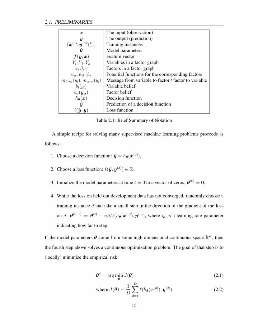
Table 2.1: Brief Summary of Notation
A simple recipe for solving many supervised machine learning problems proceeds as
follows:
1. Choose a decision function: y = hθ(x(d)).
2. Choose a loss function: ℓ(y,y(d)) ∈ R.
3. Initialize the model parameters at time t = 0 to a vector of zeros: θ(0) = 0.
4. While the loss on held out development data has not converged, randomly choose a
training instance d and take a small step in the direction of the gradient of the loss
on d: θ(t+1) = θ(t) − ηt∇ℓ(hθ(x(d)),y(d)), where ηt is a learning rate parameter
indicating how far to step.
If the model parameters θ come from some high dimensional continuous space RK , then
the fourth step above solves a continuous optimization problem. The goal of that step is to
(locally) minimize the empirical risk:
θ∗ = argminθJ(θ) (2.1)
where J(θ) =1
D
D∑
d=1
ℓ(hθ(x(d)),y(d)) (2.2)
15

2.2. NEURAL NETWORKS AND BACKPROPAGATION
Depending on the choice of decision function h and loss function ℓ, the optimization prob-
lem may or may not be convex and piecewise constant. Regardless, we can locally opti-
mize it using stochastic gradient descent, the simple first-order optimization method given
in steps 3-4, which takes many small steps in the direction of the gradient for a single
randomly chosen training example.
Road Map for this Section Throughout this section, we will discuss various forms for
the decision function h (Section 2.2 and Section 2.3), the loss function ℓ, details about
stochastic optimization and regularization (Section 2.4), other objective functions (Sec-
tion 2.3.4), and how to compute gradients efficiently (Section 2.2.2). We will give special
attention to graphical models (Section 2.3) in which θ are the parameters of a probabilistic
model.
2.2 Neural Networks and Backpropagation
This section describes neural networks, considering both their topology (Section 2.2.1) and
how to compute derivatives of the functions they define (Section 2.2.2 and Section 2.2.3).
While other more thorough treatments of neural networks can be found in the literature, we
go into some detail here in order to facilitate connections with backpropagation through in-
ference algorithms for graphical models—considered later in this chapter (Section 2.3.4.4).
The material presented here acts as a supplement to later uses of backpropagation such
as in Chapter 4 for training of a hybrid graphical model / neural network, and in Chapter 5
and Chapter 6 for approximation-aware training.
2.2.1 Topologies
A feed-forward neural network (Rumelhart et al., 1986) defines a decision function y =
hθ(x) where x is termed the input layer and y the output layer. A feed-forward neural
16

2.2. NEURAL NETWORKS AND BACKPROPAGATION
(F) LossJ = 1
2(y − y(d))2
(E) Output (sigmoid)y = 1
1+exp(−b)
(D) Output (linear)b =
∑Dj=0 βjzj
(C) Hidden (sigmoid)zj =
11+exp(−aj) , ∀j
(B) Hidden (linear)aj =
∑Mi=0 αjixi, ∀j
(A) InputGiven xi, ∀i
Figure 2.1: Feed-forward topology of a 2-layer neural network.
network has a statically defined topology. Figure 2.1 shows a simple 2-layer neural network
consisting of an input layer x, a hidden layer z, and an output layer y. In this example, the
output layer is of length 1 (i.e. just a single scalar y). The model parameters of the neural
network are a matrix α and a vector β.
The feed-forward computation proceeds as follows: we are given x as input (Fig. 2.1
(A)). Next, we compute an intermediate vector a, each entry of which is a linear combi-
nations of the input (Fig. 2.1 (B)). We then apply the sigmoid function σ(a) = 11+exp(a)
element-wise to obtain z (Fig. 2.1 (C)). The output layer is computed in a similar fashion,
first taking a linear combination of the hidden layer to compute b (Fig. 2.1 (D)) then apply-
ing the sigmoid function to obtain the output y (Fig. 2.1 (E)). Finally we compute the loss
J (Fig. 2.1 (F)) as the squared distance to the true value y(d) from the training data.
We refer to this topology as an arithmetic circuit. It defines both a function mapping
x to J , but also a manner of carrying out that computation in terms of the intermediate
17

2.2. NEURAL NETWORKS AND BACKPROPAGATION
quantities a, z, b, y. Which intermediate quantities to use is a design decision. In this
way, the arithmetic circuit diagram of Figure 2.1 is differentiated from the standard neural
network diagram in two ways. A standard diagram for a neural network does not show this
choice of intermediate quantities nor the form of the computations.
The topologies presented in this section are very simple. However, we will later (Chap-
ter 5) how an entire algorithm can define an arithmetic circuit.
2.2.2 Backpropagation
The backpropagation algorithm (Rumelhart et al., 1986) is a general method for computing
the gradient of a neural network. Here we generalize the concept of a neural network to
include any arithmetic circuit. Applying the backpropagation algorithm on these circuits
amounts to repeated application of the chain rule. This general algorithm goes under many
other names: automatic differentiation (AD) in the reverse mode (Automatic Differentiation
of Algorithms: Theory, Implementation, and Application 1991), analytic differentiation,
module-based AD, autodiff, etc. Below we define a forward pass, which computes the
output bottom-up, and a backward pass, which computes the derivatives of all intermediate
quantities top-down.
Chain Rule At the core of the backpropagation algorithm is the chain rule. The chain
rule allows us to differentiate a function f defined as the composition of two functions g
and h such that f = (g ◦h). If the inputs and outputs of g and h are vector-valued variables
then f is as well: h : RK → RJ and g : RJ → RI ⇒ f : RK → RI . Given an input
vector x = {x1, x2, . . . , xK}, we compute the output y = {y1, y2, . . . , yI}, in terms of an
intermediate vector u = {u1, u2, . . . , uJ}. That is, the computation y = f(x) = g(h(x))
can be described in a feed-forward manner: y = g(u) and u = h(x). Then the chain rule
18

2.2. NEURAL NETWORKS AND BACKPROPAGATION
must sum over all the intermediate quantities.
dyidxk
=J∑
j=1
dyiduj
dujdxk
, ∀i, k (2.3)
If the inputs and outputs of f , g, and h are all scalars, then we obtain the familiar form
of the chain rule:
dy
dx=dy
du
du
dx(2.4)
Binary Logistic Regression Binary logistic regression can be interpreted as a arithmetic
circuit. To compute the derivative of some loss function (below we use cross-entropy) with
respect to the model parameters θ, we can repeatedly apply the chain rule (i.e. backprop-
agation). Note that the output q below is the probability that the output label takes on the
value 1. y∗ is the true output label. The forward pass computes the following:
J = y∗ log q + (1− y∗) log(1− q) (2.5)
where q = Pθ(Yi = 1|x) = 1
1 + exp(−∑Dj=0 θjxj)
(2.6)
The backward pass computes dJdθj
∀j.
Forward Backward
J = y∗ log q + (1− y∗) log(1− q)dJ
dq=y∗
q+
(1− y∗)
q − 1
q =1
1 + exp(−a)dJ
da=dJ
dq
dq
da,dq
da=
exp(−a)(exp(−a) + 1)2
a =D∑
j=0
θjxjdJ
dθj=dJ
da
da
dθj,da
dθj= xj
dJ
dxj=dJ
da
da
dxj,da
dxj= θj
19

2.2. NEURAL NETWORKS AND BACKPROPAGATION
2-Layer Neural Network Backpropagation for a 2-layer neural network looks very simi-
lar to the logistic regression example above. We have added a hidden layer z corresponding
to the latent features of the neural network. Note that our model parameters θ are defined
as the concatenation of the vector β (parameters for the output layer) with the vectorized
matrix α (parameters for the hidden layer).
Forward Backward
J = y∗ log q + (1− y∗) log(1− q)dJ
dq=y∗
q+
(1− y∗)
q − 1
q =1
1 + exp(−b)dJ
db=dJ
dy
dy
db,dy
db=
exp(−b)(exp(−b) + 1)2
b =D∑
j=0
βjzjdJ
dβj=dJ
db
db
dβj,db
dβj= zj
dJ
dzj=dJ
db
db
dzj,db
dzj= βj
zj =1
1 + exp(−aj)dJ
daj=dJ
dzj
dzjdaj
,dzjdaj
=exp(−aj)
(exp(−aj) + 1)2
aj =M∑
i=0
αjixidJ
dαji=dJ
daj
dajdαji
,dajdαji
= xi
dJ
dxi=dJ
daj
dajdxi
,dajdxi
=D∑
j=0
αji
Notice that this application of backpropagation computes both the derivatives with respect
to each model parameter dJdαji
and dJdβj
, but also the partial derivatives with respect to each
intermediate quantity dJdaj, dJdzj, dJdb, dJdy
and the input dJdxi
.
2.2.3 Numerical Differentiation
Numerical differentiation provides a convenient method for testing gradients computed by
backpropagation. The centered finite difference approximation is:
∂
∂θiJ(θ) ≈ (J(θ + ϵ · di)− J(θ − ϵ · di))
2ϵ(2.7)
20

2.3. GRAPHICAL MODELS
where di is a 1-hot vector consisting of all zeros except for the ith entry of di, which has
value 1. Unfortunately, in practice, it suffers from issues of floating point precision. There-
fore, it is typically only appropriate to use this on small examples with an appropriately
chosen ϵ.
2.3 Graphical Models
This section describes some of the key aspects of graphical models that will be used
throughout this thesis. This section contains many details about model representation,
approximate inference, and training that form the basis for the SRL models we consider
in Chapter 3. Further, these methods are considered the baseline against which we will
compare our approximation-aware training in Chapter 5 and Chapter 6. The level of detail
presented here is intended to address the interests of a practitioner who is hoping to explore
these methods in their own research.
2.3.1 Factor Graphs
A graphical model defines a probability distribution pθ over a set of V predicted variables
{Y1, Y2, . . . , YV } conditioned on a set of observed variables {X1, X2, . . . , }. We will con-
sider distributions of the form:
p(y | x) = 1
Z(x)
∏
α∈Fψα(yα,x) (2.8)
Each α ∈ F defines the indices of a subset of the variables α ⊂ {1, . . . , V }. For each α,
there is a corresponding potential function ψα, which gives a non-negative score to the
variable assignments yα = {yα1 , yα2 , . . . yα|α|}. The partition function Z(x) is defined
21
2.3. GRAPHICAL MODELS
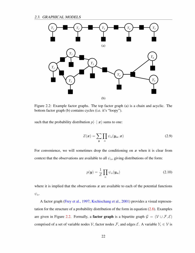
Y1 ψ2 Y2 ψ4 Y3 ψ6 Y4 ψ8 Y5
ψ1 ψ3 ψ5 ψ7 ψ9
(a)
Y1
ψ1
ψ2
Y2
ψ3
ψ4
Y3
ψ5
ψ6
Y4
ψ7
ψ8
Y5
ψ9
Y6
ψ10
Y7
ψ12
ψ11 ψ11
(b)
Figure 2.2: Example factor graphs. The top factor graph (a) is a chain and acyclic. Thebottom factor graph (b) contains cycles (i.e. it’s “loopy”).
such that the probability distribution p(· | x) sums to one:
Z(x) =∑
y
∏
α
ψα(yα,x) (2.9)
For convenience, we will sometimes drop the conditioning on x when it is clear from
context that the observations are available to all ψα, giving distributions of the form:
p(y) =1
Z
∏
α
ψα(yα) (2.10)
where it is implied that the observations x are available to each of the potential functions
ψα.
A factor graph (Frey et al., 1997; Kschischang et al., 2001) provides a visual represen-
tation for the structure of a probability distribution of the form in equation (2.8). Examples
are given in Figure 2.2. Formally, a factor graph is a bipartite graph G = (V ∪ F , E)
comprised of a set of variable nodes V , factor nodes F , and edges E . A variable Yi ∈ V is
22

2.3. GRAPHICAL MODELS
said to have neighbors N (Yi) = {α ∈ F : i ∈ α}, each of which is a factor α. Here we
have overloaded α to denote both the factor node, and also the index set of its neighboring
variables N (α) ⊂ V . The graph defines a particular factorization of the distribution pθ
over variables Y . The name factor graph highlights an important consideration throughout
this thesis: how a probability distribution factorizes into potential functions will determine
greatly the extent to which we can apply our machine learning toolbox to learn its parame-
ters and make predictions with it.
The model form in equation (2.10) described above is sufficiently general to capture
Markov random fields (MRF) (undirected graphical models), and Bayesian networks (di-
rected graphical models)—though for the latter the potential functions ψα must be con-
strained to sum-to-one. Trained discriminatively, without such a constraint, the distribution
in equation (2.8) corresponds to a conditional random field (CRF) (Lafferty et al., 2001).
2.3.2 Minimum Bayes Risk Decoding
From our earlier example, we noted that it is sometimes desirable to define a decision func-
tion hθ(x), which takes an observation x and predicts a single y. However, the graphical
models we describe in this section instead define a probability distribution pθ(y | x) over
the space of possible values y. So how should we best select a single one?
Given a probability distribution pθ and a loss function ℓ(y,y), a minimum Bayes risk
(MBR) decoder returns the variable assignment y with minimum expected loss under the
model’s distribution (Bickel and Doksum, 1977; Goodman, 1996).
hθ(x) = argminy
Ey∼pθ(·|x)[ℓ(y,y)] (2.11)
= argminy
∑
y
pθ(y | x)ℓ(y,y) (2.12)
Consider an example MBR decoder. Let ℓ be the 0-1 loss function: ℓ(y,y) = 1− I(y,y),
where I is the indicator function. That is, ℓ returns loss of 0 if y = y and loss of 1 otherwise.
23

2.3. GRAPHICAL MODELS
Regardless of the form of the probability distribution, equation (2.12) reduces to:
hθ(x) = argminy
∑
y
pθ(y | x)(1− I(y,y)) (2.13)
= argmaxy
pθ(y | x) (2.14)
That is, the MBR decoder hθ(x) will return the most probable variable assignment accord-
ing to the distribution. Equation (2.14) corresponds exactly to the MAP inference problem
of equation (2.18).
For other choices of the loss function ℓ, we obtain different decoders. Let our loss
function be Hamming loss, ℓ(y,y) =∑V
i=1(1 − I(yi, yi)). For each variable the MBR
decoder returns the value with highest marginal probability:
yi = hθ(x)i = argmaxyi
pθ(yi | x) (2.15)
where pθ(yi | x) is the variable marginal given in equation (2.16).
2.3.3 Approximate Inference
Given a probability distribution defined by a graphical model, there are three common
inference tasks:
Marginal Inference The first task of marginal inference computes the marginals of
the variables:
pθ(yi | x) =∑
y′:y′i=yi
pθ(y′ | x) (2.16)
24

2.3. GRAPHICAL MODELS
and the marginals of the factors
pθ(yα | x) =∑
y′:y′α=yα
pθ(y′ | x) (2.17)
Partition Function The second task is that of computing the partition function Z(x)
given by equation (2.9). Though the computation is defined as the sum over all
possible assignments to the variables Y , it can also be computed as a function of
the variable (2.16) and factor marginals (2.17) as we will see in Section 2.3.3.3.
MAP Inference The third task computes the variable assignment y with highest prob-
ability. This is also called the maximum a posteriori (MAP) assignment.
y = argmaxy
pθ(y | x) (2.18)
2.3.3.1 Belief Propagation
The belief propagation (BP) (Pearl, 1988) algorithm can be used to compute variable
marginals pθ(yi | x) and factor marginals pθ(yα | x) when the factor graph correspond-
ing to pθ is acyclic. BP is a message passing algorithm and defines the following update
equations for messages from variables to factors (i → α) and from factors to variables
(α → i):
mi→α(yi) =1
κi→α
∏
β∈N (i)\αmβ→i(yi) (2.19)
mα→i(yi) =1
κα→i
∑
yα∼yiψα(yα)
∏
j∈N (α)\imj→α(yi) (2.20)
where N (i) and N (α) denote the neighbors of yi and α respectively, and where yα ∼ yi
is standard notation to indicate that yα ranges over all assignments to the variables partic-
ipating in the factor α for which the ith variable has value yi. Above, κi→α and κα→i are
25

2.3. GRAPHICAL MODELS
normalization constants ensuring that the vectors mi→α and mα→i sum to one. BP also
defines update equations for beliefs at the variables and factors:
bi(yi) =1
κi
∏
α∈N (i)
m(tmax)α→i (yi) (2.21)
bα(yα) =1
καψα(yα)
∏
i∈N (α)
m(tmax)i→α (yi) (2.22)
where κi and κα ensure the belief vectors bi and bα are properly normalized.
There are several aspects of the form of these update equations to notice: (1) The mes-
sages are cavity products. That is, they compute the product of all but one of the incoming
messages to a variable or factor node. This is in contrast to the beliefs, which include
a product of all incoming messages. (2) The message vectors mi→α and mα→i always
define a distribution over a variable yi regardless of whether they are sent to or from the
variable yi. (3) The update equations must be executed in some order, a topic we take up
below.
There are two basic strategies for executing BP:
1. An asynchronous (serial) update order picks the next edge e ∈ E , where e may be
a variable-to-factor or factor-to-variable edge. It then executes the message update
equations (2.19) and (2.20) for that edge so that the corresponding message vector is
updated based on the current values of all the other messages.
2. By contrast, a synchronous (parallel) update strategy runs all the update equations at
once ((2.19) and (2.20)) caching the results in temporary storage. Once the message
vectors for all edges e ∈ E have been stored, it sets the current values of the messages
to be the ones just computed. That is, all the messages at time t are computed from
those at time t− 1.
An update of every message constitutes an iteration of BP. In practice, the asynchronous
approach tends to converge faster than the synchronous approach. Further, for an asyn-
26
2.3. GRAPHICAL MODELS
chronous order, there are a variety of methods for choosing which message to send next
(e.g. (Elidan et al., 2006)) that can greatly speed up convergence.
The messages are said to have converged when they stop changing. When the factor
graph is acyclic, the algorithm is guaranteed to converge after a finite number of iterations
(assuming every message is sent at each iteration).
The BP algorithm described above is properly called the sum-product BP algorithm
and performs marginal inference. Next we consider a variant for MAP inference.
Max-product BP The max-product BP algorithm computes the MAP assignment ((2.18))
for acyclic factor graphs. It requires only a slight change to the BP update equations given
above. Specifically we replace equation (2.20) with the following:
mα→i(yi) =1
κα→i
maxyα∼yi
ψα(yα)∏
j∈N (α)\imj→α(yi) (2.23)
Notice that the new equation ((2.23)) is identical to sum-product version ((2.20)) except
that the summation∑
yα∼yi was replaced with a maximization maxyα∼yi . Upon conver-
gence, the beliefs computed by this algorithm are max-marginals. That is, bi(yi) is the
(unnormalized) probability of the MAP assignment under the constraint Yi = yi. From the
max-marginals the MAP assignment is given by:
y∗i = argmaxyi
bi(yi), ∀i (2.24)
2.3.3.2 Loopy Belief Propagation
Loopy belief propagation (BP) (Murphy et al., 1999) is an approximate inference algorithm
for factors with cycles (i.e. “loopy” factor graphs as shown in Figure 2.2). The form of the
algorithm is identical to that of Pearl (1988)’s belief propagation algorithm described in
Section 2.3.3.1 except that we ignore the cycles in the factor graph. Notice that BP is
fundamentally a local message passing algorithm: each message and belief is computed
27

2.3. GRAPHICAL MODELS
only as a product of (optionally) a potential function and messages that are local (i.e. being
sent to) to a single variable or factor. The update equations know nothing about the cyclicity
(or lack thereof) of the factor graph.
Accordingly, loopy BP runs the message update equations ((2.19) and (2.20)) using one
of the update orders described in Section 2.3.3.1. The algorithm may or may not converge,
accordingly it is typically run to convergence or for a maximum number of iterations, tmax.
Upon termination of the algorithm, the beliefs are computed with the same belief update
equations ((2.21) and (2.22)). Upon termination, the beliefs are empirically a good estimate
of the true marginals—and are often used in place of true marginals in high-treewidth factor
graphs for which exact inference is intractable. Hereafter, since it recovers the algorithm
of Section 2.3.3.1 as a special case, we will use “BP” to refer to this more general loopy
sum-product BP algorithm.
2.3.3.3 Bethe Free Energy
Loopy BP is also an algorithm for locally optimizing a constrained optimization problem
(Yedidia et al., 2000):
min FBethe(b) (2.25)
s.t. bi(yi) =∑
yα∼yibα(yα) (2.26)
where the objective function is the Bethe free energy and is defined as a function of the
beliefs:
FBethe(b) =∑
α
∑
yα
bα(yα) log
[bα(yα)
ψα(yα)
]
−∑
i
(ni − 1)∑
yi
bi(yi) log bi(yi)
28

2.3. GRAPHICAL MODELS
where ni is the number of neighbors of variable Yi in the factor graph. For cyclic graphs,
if loopy BP converges, the beliefs correspond to stationary points of FBethe(b) (Yedidia
et al., 2000). For acyclic graphs, when BP converges, the Bethe free energy recovers the
negative log partition function: FBethe(b) = − logZ. This provides an effective method of
computing the partition function exactly for acyclic graphs. However, in the cyclic case,
the Bethe free energy also provides an (empirically) good approximation to − logZ.
2.3.3.4 Structured Belief Propagation
This section describes the efficient version of belief propagation described by Smith and
Eisner (2008).
The term constraint factor describes factors α for which some value of the potential
function ψα(yα) is 0—such a factor constrains the variables to avoid that configuration of
yα without regard to the assignment of the other variables. Notice that constraint factors
are special in this regard: any potential function that returns strictly positive values could
always be “outvoted” by another potential function that strongly disagrees by multiplying
in a very large or very small value.
Some factor graphs include structured factors. These are factors whose potential func-
tion ψα exhibits some interesting structure. In this section, we will consider two such fac-
tors:
1. The Exactly1 factor (Smith and Eisner, 2008) (also termed the XOR factor in Martins
et al. (2010b)) constrains exactly one of its binary variables to have value 1, and all
the rest to have value 0.
2. The PTree factor (Smith and Eisner, 2008) is defined over a set of O(n2) binary
variables that form a dependency tree over an n word sentence.
This section is about efficiently sending messages from structured factors to variables. That
is, we will consider cases where a factor α has a very large number of neighbors |N (α)|. In
29

2.3. GRAPHICAL MODELS
these cases, the naive computation of mα→i(yi) according to equation (2.20) would be pro-
hibitively expensive (i.e. exponential in the number of neighboring variables). Smith and
Eisner (2008) show how to make these computations efficient by the use of dynamic pro-
gramming. This variant of efficient loopy BP with structured factors is called structured
BP.
Smith and Eisner (2008) give two key observations that assist in these efficient compu-
tations: First, a factor has a belief about each of its variables:
bα(yi) =∑
yα∼yibα(yα) (2.27)
This is simply another variable belief computed from the factor marginal (not to be con-
fused with bi(yi) in equation (2.21) which has a different subscript). Second, an outgoing
message from a factor is the factor’s belief with the incoming message divided out:
mα→i(yi) =bα(yi)
mi→α(yi)(2.28)
This follows directly from the definition of the factor belief and the messages. Notice then
that we need only compute the factor’s beliefs about its variables bα(yi) and then we can
efficiently compute the outgoing messages.
Exactly1 Factor The potential function for the Exactly1 factor is defined as:
ψExactly1(yα) =
⎧⎪⎪⎨⎪⎪⎩
1, if ∃ exactly one j s.t. yj = ON and yk = OFF, ∀k = j
0, otherwise(2.29)
where each binary variable Yi has domain {ON, OFF}. We can compute the Exactly1 fac-
tor’s beliefs about each of its variables efficiently. Each of the parenthesized terms below
30

2.3. GRAPHICAL MODELS
needs to be computed only once for all the variables in N (α).
bα(Yi = ON) =
⎛⎝ ∏
j∈N (α)
mj→α(OFF)
⎞⎠ mi→α(ON)
mi→α(OFF)(2.30)
bα(Yi = OFF) =
⎛⎝ ∑
j∈N (α)
bα(Yj = ON)
⎞⎠− bα(Yi = ON) (2.31)
PTREE Factor The potential function for the PTREE factor is defined as:
ψα(yα) =
⎧⎪⎪⎨⎪⎪⎩
1, if yα define a valid projective dependency tree
0, otherwise(2.32)
In order to compute the factor’s variable belief efficiently, the first step is to utilize the fact
that ψ(yα) ∈ {0, 1}.
⇒ bα(yi) =∑
yα∼yi,ψ(yα)=1
∏
j∈N (α)
mj→α(yα[j]) (2.33)
(2.34)
where yα[j] is the value of variable Yj according to yα. Next given that Yi ∈ {ON, OFF}, ∀Yi ∈
N (α), we have:
⇒ bα(Yi = ON) =
⎛⎝ ∏
j∈N (α)
mj→α(OFF)
⎞⎠ ∑
yα∼yi,ψ(yα)=1
∏
j∈N (α):yα[j]=ON
mj→α(ON)
mj→α(OFF)(2.35)
and ⇒ bα(Yi = OFF) =
⎛⎝∑
yα
b(yα)
⎞⎠− bα(Yi = ON) (2.36)
The form of (2.35) exposes how an efficient dynamic programming algorithm can carry
out this computation. The initial parenthetical is simply a constant that can be multiplied
in at the end. The key is that the equation contains a sum over assignments y, which all
31

2.3. GRAPHICAL MODELS
correspond to projective dependency trees∑
yα∼yi,ψ(yα)=1
. The summands are each a product of
scores, one for each edge that is included in the tree,∏
j∈N (α):yα[j]=ON
. This sum over exponen-
tially many trees has a known polynomial time solution however.
Accordingly, Smith and Eisner (2008) first run the inside-outside algorithm where the
edge weights are given by the ratios of the messages to PTREE: m(t)i→α(ON)
m(t)i→α(OFF)
. Then they
multiply each resulting edge marginal given by inside-outside by the product of all the OFF
messages π =∏
im(t)i→α(OFF) to get the marginal factor belief bα(Yi = ON). The sum
of the weights of all the trees computed by the inside algorithm can be multiplied by π to
obtain the partition function∑
yαb(yα) which is used to compute bα(Yi = OFF) by (2.36).
Finally they divide the belief by the incoming message m(t)i→α(ON) to get the corresponding
outgoing message m(t+1)α→i (ON).
2.3.4 Training Objectives
In this section, we describe several training objectives: conditional log-likelihood (Lafferty
et al., 2001), empirical risk, and empirical risk minimization under approximations (Stoy-
anov et al., 2011). Except where it is relevant to introduce appropriate terminology, we
defer any discussion of regularization until Section 2.4.1.
2.3.4.1 Conditional Log-likelihood
When we have labeled examples Dl = {(x(d),y(d))}Dd=1, we can discriminatively train
to maximize the likelihood of the latent variables, y, conditioned on the observations, x.
This discriminative training approach is also called conditional log-likelihood (CLL) max-
imization and corresponds to the CRF training of Lafferty et al. (2001). The conditional
log-likelihood is given by:
L(θ) =D∑
d=1
log pθ(y(d) | x(d)) (2.37)
32

2.3. GRAPHICAL MODELS
where the probability is given by equation (2.8) to have the form p(y | x) = 1Z(x)
∏α∈F ψα(yα,x).
In this section, we consider a special case of models described in Section 2.3.1, where all
of the potential functions are defined so they come from the exponential family:
ψα(yα) = exp(θ · fα(yα,x)), ∀α (2.38)
where fα is a vector-valued feature function, usually of high dimension but sparse. For
factor graphs with this restriction, the CLL is:
L(θ) =D∑
d=1
(θ · f(y,x)− log
∑
y
exp(θ · f(y,x)))
(2.39)
where f(y,x) =∑
α fα(yα,x)). The derivative of the log-likelihood takes on the familiar
form from CRF training,
∂L(θ)∂θ
=D∑
d=1
(fj(y
(d),x(d))− Ey∼pθ(·|x(d))[fj(y,x(d))]
)(2.40)
=D∑
d=1
∑
α
(fα,j(y
(d),x(d))−∑
yα
pθ(yα | x(d))fα,j(yα,x(d))
)(2.41)
The first form of the derivative (2.40) shows its form to be the difference of the observed
feature counts minus the expected feature counts. The second form (2.41) shows that it can
be computed easily given the factor marginals from equation (2.17).
In practice, the exact marginals needed to compute this derivative can be replaced with
an approximation, such as the beliefs from loopy BP (Section 2.3.3.2). This gives the
gradient of a different objective function, termed the surrogate log-likelihood (Wainwright,
2006). We discuss this setting in greater detail in Chapter 5.
33

2.3. GRAPHICAL MODELS
2.3.4.2 CLL with Latent Variables
Suppose instead we want to maximize the likelihood of a subset of the variables, treating
the others as latent. In this case, we have a probability distribution of the form:
pθ(y) =∑
z
pθ(y, z) =∑
z
1
Z
∏
α
ψα(yα, zα) (2.42)
where y are values of the predicted variables, z are values of the latent variables, and the
dependence on x is not shown. This distribution can be rewritten in terms of two partition
functions:
pθ(y) =Z(y)
Z(2.43)
where
Z(y) =∑
z
∏
α
ψα(yα, zα) (2.44)
(2.45)
The derivative of the conditional log-likelihood in this case reduces to the following differ-
ence of expectations:
∂L(θ)∂θ
=D∑
d=1
(Ez∼pθ(·|y(d))[fj(y
(d), z)]− Ey,z∼pθ(·,·)[fj(y, z)])
(2.46)
=D∑
d=1
∑
α
(∑
zα
pθ(zα | y(d))fα,j(y(d)α , zα)−
∑
yα,zα
pθ(yα, zα)fα,j(yα, zα)
)
(2.47)
where p(zβ|y) is the marginal distribution over zβ conditioned on a fixed assignment to
the variables y. In practice, this marginal is computed by making a copy of the original
factor graph and clamping the values of y, then running inference to obtain the marginals
34

2.3. GRAPHICAL MODELS
of zβ . The other marginal pθ(yα, zα) gives the distribution of the joint assignment to yα
and zα. See Sutton and McCallum (2007) for additional details about this latent variable
case.
2.3.4.3 Empirical Risk Minimization
The choice to minimize empirical risk in our simple recipe from Section 2.1.1 is a well
motivated one. In fact, we usually aim to find parameters θ∗ that minimize expected loss
on the true data distribution over sentence/parse pairs (X, Y ):
θ∗ = argminθ
E[ℓ(hθ(X), Y )] (2.48)
Since the true data distribution is unknown in practice, we estimate the objective by the
expected loss over the training sample, {(x(d),y(d))}Dd=1. This estimate is called the em-
pirical risk:
θ∗ = argminθ
1
D
D∑
d=1
ℓ(hθ(x(d)),y(d)) (2.49)
There are two problems associated with this objective function. First, the optimization itself
can be difficult depending on the choice of loss function ℓ. The risk could be nonconvex
and piecewise constant—properties which cause problems for most typical first- or second-
order optimization algorithms, such as the ones we will discuss in Section 2.4. Second, if
we do successfully minimize it, the model may overfit the training data. For this reason,
we usually minimize the regularized empirical risk.
θ∗ = argminθ
1
D
(r(θ) +
D∑
d=1
ℓ(hθ(x(d)),y(d))
)(2.50)
35

2.4. CONTINUOUS OPTIMIZATION
where r(θ) is a regularization function that discourages large (absolute values) or non-zero
values in θ. Examples are given in Section 2.4.1.
2.3.4.4 Empirical Risk Minimization Under Approximations
When inference is exact and the decoder and loss function are differentiable, it is possible to
do empirical risk minimization (2.49) and regularized empirical risk minimization (2.50).
Sometimes the derivatives are simple enough to be computed by hand—for neural networks
they are computed by backpropagation.
Stoyanov et al. (2011) and Stoyanov and Eisner (2012) introduce empirical risk min-
imization under approximations (ERMA), which treats the entire system including ap-
proximate inference, decoding, and loss as if it were an arithmetic circuit. That arithmetic
circuit (up to but not including loss) defines some decision function hθ(x) and its deriva-
tive can be computed by backpropagation. Figure 2.3 depicts such an arithmetic circuit.
For a differentiable loss, Stoyanov et al. (2011) train the system to minimize empirical
risk—taking the approximations into account.
We defer a more detailed discussion of this method until Chapter 5.
2.4 Continuous Optimization
Recent advances in stochastic optimization and online learning have been critical to the
recent success of large-scale machine learning. The approaches considered in this thesis
have similarly benefitted from these advances. Only on very rare occasions is it advisable
to treat optimization as a black box that takes a function and returns a local optimum—on
the contrary, one should open the black box to know what’s inside before using it blindly.
To choose an effective optimization method, we consider three desiderata: (1) efficient
use of first-order gradient computations, (2) sparse updates with regularization, and (3)
low bounds on regularized regret. In this section, we discuss stochastic gradient descent
36

2.4. CONTINUOUS OPTIMIZATION
(E) Decode and LossJ(θ;x,y∗) = . . .
(D) Beliefsbi(yi) = . . ., bα(yα) = . . .
(C) Messages at time tmax
m(tmax)i→α (yi) = . . .,
m(tmax)α→i (yi) = . . .
· · ·
(C) Messages at time tm
(t)i→α(yi) = . . .,
m(t)α→i(yi) = . . .
· · ·
(C) Messages at time t = 1
m(1)i→α(yi) = . . .,
m(1)α→i(yi) = . . .
(A) Compute Potentialsψα(yα) = exp(θ · f(yα,x))
(B) Initial Messagesm
(0)i→α(yi) = 1
m(0)α→i(yi) = 1
Figure 2.3: Feed-forward topology of inference, decoding, and loss according to ERMA(Stoyanov et al., 2011).
(SGD), mirror descent (MD) (Nemirovsky and Yudin, 1983; Beck and Teboulle, 2003),
Composite Mirror Descent (COMID) (Duchi et al., 2010a), and AdaGrad (Duchi et al.,
2010b; Duchi et al., 2011). Our treatment of these algorithms is very brief and primarily
aims to explain how our desiderata are met by AdaGrad with Composite Mirror Descent
and ℓ22-regularization via lazy updates.
The methods are presented in a tutorial style. The success of this thesis certainly de-
pends on effective algorithms for continuous optimization. However, the main contribu-
tions can certainly be understood without the details discussed here. AdaGrad will be put
37

2.4. CONTINUOUS OPTIMIZATION
to use repeatedly for supervised and semi-supervised learning in Chapter 3, Chapter 4,
Chapter 5, and Chapter 6.
2.4.1 Online Learning and Regularized Regret
Here we highlight an important connection between regularized loss minimization (the
setting of the optimization problems solved in this thesis) and online learning.
Regularized Loss Minimization Throughout this thesis, our focus is generally on the
problem of regularized loss minimization for some loss function fd(θ), which is defined
in terms of the training example pair (x(d),y(d)). This gives us an optimization problem
based on the regularized loss R(θ).
θ∗ = argminθ∈Θ
R(θ) where R(θ) =1
D
D∑
d=1
Jd(θ) + r(θ) (2.51)
where θ ∈ Rd are the model parameters, Jd : Θ → R is a loss function, and r : Θ → R is
a regularization function. Θ is a convex set of possible parameters. Jd is differentiable and
convex. r is convex. Example regularizers include
• ℓ1-regularization, r(θ) = λ||θ||1
• ℓ22-regularization, r(θ) = λ2||θ||22. This is equivalent to a spherical Gaussian prior
on the parameters where λ is the inverse variance. We also informally refer to this
regularizer as ℓ2 in order to better coincide with the NLP literature.
The hyperparameter λ trades off between the regularizer and loss and is typically tuned on
held out data. Example loss functions include conditional log-likelihood (Section 2.3.4.1)
or empirical risk (Section 2.3.4.3).
Online Learning In the online learning setting, we choose a sequence of parameters
θ(t) for time steps t = 1, 2, 3, . . .. At each time step t, an adversary gives us another loss
38

2.4. CONTINUOUS OPTIMIZATION
function Jt and we receive the loss Jt(θ(t)). The goal is then to ensure that the total loss
up to each time step T ,∑T
t=1 Jt(θ(t)), is not much worse (larger) than minθ
∑Tt=1 Jt(θ),
which is the smallest total loss of any fixed set of parameters θ chosen retrospectively. This
is the regret:
RT :=T∑
t=1
Jt(θ(t))−min
θ
T∑
t=1
Jt(θ) (2.52)
The regularized regret simply incorporates the regularizer r.
RT :=T∑
t=1
(Jt(θ(t)) + r(θ(t)))−min
θ
T∑
t=1
(Jt(θ)− r(θ)) (2.53)
The goal is then to choose an optimization algorithm that bounds this (regularized) regret.
Connection Consider an online learning setting where at time step t we randomly select
a training example d, defining the loss function Jt = Jd to be the loss function for that train-
ing example. If our optimization algorithm bounds the regularized regret (equation (2.53)),
intuitively it will also be attempting to minimize the regularized loss (equation (2.51)).
Cesa-Bianchi et al. (2004) make an even stronger claim: given a bound on equation (2.53)
we can obtain convergence rate and generalization bounds for equation (2.51). More to
the point, if optimization algorithm has a tight bound on the regularized regret, we will
converge to (local) optimum faster.
2.4.2 Online Learning Algorithms
Next we consider a sequence of four online learning algorithms—each of which extends
the previous—with the goal of providing a clearer understanding of the development of the
AdaGrad-COMID algorithm.
39

2.4. CONTINUOUS OPTIMIZATION
2.4.2.1 Stochastic Gradient Descent
Stochastic gradient descent (SGD) defines a simple update for each iteration.
θ(t+1) = θ(t) − ηt(J′t(θ
(t)) + r′(θ(t))) (2.54)
where J ′t(θ) is the gradient of Jt or one of its subgradients at point θ, and r′(θ) is equiva-
lently a gradient or subgradient of r(θ). Note that we have departed from the notation of
∇Jt(θ) for gradients, used elsewhere in this thesis, for clarity in the introduction of subse-
quent optimization algorithms. Intuitively, SGD takes a small step in the direction of the
gradient of the regularized loss. Typically, to ensure convergence, the learning rate ηt is
chosen to decay over time.
2.4.2.2 Mirror Descent
Let ϕt = Jt+r denote the sum of the loss function and regularizer at time t. Intuitively, the
Mirror Descent algorithm (Nemirovsky and Yudin, 1983; Beck and Teboulle, 2003) update
given below minimizes a linear approximation of the function ϕt at the current parameters
θ(t) while ensuring that the next θ(t+1) is close to θ(t). Hereafter, for vectors a and b, we
use ⟨a, b⟩ to denote their dot product. The update for Mirror Descent is:
θ(t+1) = argminθ∈Θ
η⟨ϕ′t(θ
(t)),θ − θ(t)⟩+Bψ(θ,θ
(t)) (2.55)
= argminθ∈Θ
η⟨J ′t(θ
(t)) + r′(θ(t)),θ − θ(t)⟩+Bψ(θ,θ
(t)) (2.56)
where η is a learning rate parameter, ϕ′t is a (sub)gradient of ϕt, Bψ is a Bregman di-
vergence, and ψ is a carefully chosen function (more discussion below). The Bregman
divergence for ψ is defined as:
Bψ(w,v) = ψ(w)− ψ(v)− ⟨ψ′(v),w − v⟩ (2.57)
40

2.4. CONTINUOUS OPTIMIZATION
where ψ′ is the gradient of ψ. Duchi et al. (2010a) require that ψ have two properties: (a)
continuously differentiable, and (b) α-strongly convex with respect to a norm ||·|| on the set
of possible model parameters Θ. An example of such a function would be ψ(w) = 12||w||22.
2.4.2.3 Composite Objective Mirror Descent
Composite objective mirror descent (COMID) (Duchi et al., 2010a) uses the following
update.
θ(t+1) = argminθ∈Θ
η⟨J ′t(θ
(t)),θ − θ(t)⟩+ ηr(θ) +Bψ(θ,θ
(t)) (2.58)
This update is identical to that of Mirror Descent in equation (2.56), except that r(θ) is not
linearized, but instead included directly in the minimization. Duchi et al. (2010a) give a
O(√T ) bound for the regret in the general case, and a O(log T ) bound when Jt(θ) + r(θ)
is strongly convex. Note that we have not yet specified exactly how one would compute the
argmin above. For many choices of r(θ) and ψ(w), this update has a closed form. We will
give such a derived algorithm for AdaGrad-COMID below.
2.4.2.4 AdaGrad
The AdaGrad family of algorithms (Duchi et al., 2010b; Duchi et al., 2011) is defined in
two forms. The first is based on Composite Objective Mirror Descent, and is our focus
in this section. The second is derived similarly from Regularized Dual Averaging (Xiao,
2009), though we do not describe it here. The updates for both cases are defined for a
very careful choice of ψ, which is adapted over time such that it is sensitive to the data.
AdaGrad-COMID starts with the update from equation (2.58). The first change is that it
defines a different ψ for each time step t. That is we replace ψ in equation (2.58) with ψt.
The key contribution of AdaGrad is defining the proximal functions ψt to be the squared
41

2.4. CONTINUOUS OPTIMIZATION
Mahalanobis norm:
ψt(θ) =1
2⟨θ, Htθ⟩ (2.59)
where Ht is a diagonal matrix defined such that each Ht,i,i = δ +√∑t
s=1(f′s(θ)i)
2 is a
smoothed version of the square root of the sum of the squares of the ith element of the
gradient over all time steps up to t. With this definition of ψt, the update in equation (2.58)
can then be simplified to:
θ(t+1) = argminθ∈Θ
⟨ηJ ′
t(θ(t))−Htθ
(t),θ⟩+ ηr(θ) +
1
2⟨θ, Htθ⟩ (2.60)
Intuitively, large partial derivatives along dimension i will lead to smaller (more conserva-
tive) steps in that dimension.
Derived Algorithms for AdaGrad-COMID Finally, the derived algorithms for AdaGrad-
COMID for the regularizers from Section 2.4.1, can be given as closed form updates to the
parameters. For the ℓ1-regularizer, r(θ) = λ||θ||1, we have the following update.
θ(t+1)i = sign
(θ(t)i − η
Ht,i,i
gt,i
)[⏐⏐⏐⏐θ(t)i − η
Ht,i,i
gt,i
⏐⏐⏐⏐−λη
Ht,i,i
]
+
(2.61)
where [x]+ = max(0, x), sign(x) is the sign of x, and gt,i is shorthand for the ith element
of f ′t(θ).
For the ℓ22-regularizer, r(θ) = λ2||θ||22, we have the following update.
θ(t+1)i =
Ht,i,iθ(t)i − ηgt,i
ηλδ +Ht,i,i
(2.62)
where the hyperparameter δ helps deal with the initially noisy values in Ht,i,i and typically
takes a small positive value ≤ 1.
42

2.4. CONTINUOUS OPTIMIZATION
Regret Bound The same O(√T ) and O(log T ) bounds apply to AdaGrad-COMID be-
cause it is just a special case of the COMID algorithm. However, Duchi et al. (2011) further
prove that the bound on the regret they obtain is as good as the best possible choice for ψ
in hindsight.
AdaGrad-COMID with Lazy Updates Of importance to this work is the fact that these
algorithms can be modified to support lazy updates of the model parameters (Duchi et
al., 2010b; Duchi et al., 2011). This is important since the gradients we compute J ′t(θ) are
based on a single training example d and are therefore very sparse (e.g. only a few thousand
parameters out of tens of millions). However, due to the regularizer every parameter θi
would be updated at each time step.
In the lazy-updates version of AdaGrad-COMID (Duchi et al., 2010b; Duchi et al.,
2011), the update is only applied in equation (2.62) to those parameters θi where the ith
value in J ′t(θ) is non-zero. For all the other parameters the update θ(t+1)
i = θ(t)i is used. For
model parameter θi, let t0 denote the last time step at which the ith value of the gradient
J ′t0(θ) was non-zero. Then we can lazily compute θ(t)i from θ
(t0)i as below:
θ(t)i = θ
(t0)i
(Ht,i,i
ηλδ +Ht0,i,i
)(t−t0)(2.63)
2.4.2.5 Parallelization over Mini-batches
Above, we assumed that Jt(θ) = Jd(θ) for a single randomly chosen example d from our
training dataset. Alternatively, we can let Jt to be the average over a randomly chosen
mini-batch of examples, {d1, d2, . . . , dK}: Jt(θ) = 1K
∑Kk=1 Jdk(θ). If we view the train-
ing example d and the minibatch {d1, d2, . . . , dK} as random variables, then the expected
values of either gradient is that of the full batch gradient:
E[Jd(θ)] = E
[1
K
K∑
k=1
Jdk(θ)
]=
1
D
D∑
d=1
Jd(θ) (2.64)
43

2.4. CONTINUOUS OPTIMIZATION
Often, it is preferable to use mini-batches because the gradients are a lower variance esti-
mate of the full batch gradient. In this thesis, we prefer the mini-batch approach because
it allows for a trivial method of parallelization during training: each gradient Jdk(θ) can
be computed independently on a separate thread with shared-memory access to the model
parameters. Whenever the gradient computation dominates the computation time, this can
be a very effective method of parallelization. This is the case in the models we consider
for which feature extraction and inference are typically more computationally expensive
than the other non-parallelized SGD computations. In practice, we typically choose the
mini-batch size K to be 2-3 times the number of threads available.
44

Chapter 3
Latent Variables and Structured Factors
The primary goal of this chapter1—within the broader context of the thesis—is to motivate
the use of joint modeling in low-resource settings. Our focus is the interface of syntax and
semantics. To that end, we choose a specific task, semantic role labeling (SRL), for which
there is strong evidence that additional structure, in the form of syntactic dependencies, is
highly informative.
A possible criticism of this choice is that SRL does not represent an end-task. Ideally,
to establish the dominance of joint modeling in the low-resource setting, we would pick
a field such as computer vision, and jointly model all the tasks that field believes to be
important and relevant—or at least as many as the field has data for. Here we only aim to
motivate such a framework for joint modeling. We choose the task of low-resource SRL
for several reasons:
1. A wealth of prior work has been invested into building state-of-the-art models with-
out fancy new machinery (e.g. neural nets). Later in this thesis will explore such
techniques (Chapter 4 and Chapter 6), but here we restrict to simple log-linear mod-
els.
2. SRL permits us to define a joint model of syntax/semantics for which exact inference
1A previous version of this work was presented in Gormley et al. (2014).
45

3.1. INTRODUCTION
is possible. Though we later address the issue of learning with approximate inference
(Chapter 5), we can focus here on the simpler case of maximum likelihood estimation
with exact inference.
3. Third, the question of whether joint modeling is beneficial for the high-resource set-
ting has already been studied. Specifically, the results from the CoNLL-2009 shared
task (Hajic et al., 2009) and some subsequent work (Lluıs et al., 2013) demonstrated
that the tradeoff of a richer model with more challenging inference vs. the rich fea-
tures of a pipeline but with easy inference remains unclear. We do not seek to clarify
this tradeoff for the high-resource setting, but instead aim to demonstrate that the
benefits of joint modeling in the low-resource SRL setting are much clearer.
Note that the low-resource setting is one that has been explored before (Boxwell et al.,
2011; Naradowsky et al., 2012a). However, the empirical studies to date leave our question
unanswered: is joint modeling worth it? This is because prior work did not include a
controlled comparison of joint and pipelined systems in the low-resource setting.
We begin to address this question by exploring the extent to which high-resource man-
ual annotations such as treebanks are necessary for the task of semantic role labeling (SRL).
We examine how performance changes without syntactic supervision, comparing both joint
and pipelined methods to induce latent syntax. This work highlights a new application of
unsupervised grammar induction and demonstrates several approaches to SRL in the ab-
sence of supervised syntax. Our best models obtain competitive results in the high-resource
setting and state-of-the-art results in the low-resource setting, reaching 72.48% F1 averaged
across languages.
3.1 Introduction
The goal of semantic role labeling (SRL) is to identify predicates and arguments and label
their semantic contribution in a sentence. Such labeling defines who did what to whom,
46

3.1. INTRODUCTION
when, where and how. For example, in the sentence “The kids ran the marathon”, ran
assigns a role to kids to denote that they are the runners; and a distinct role to marathon
since it denotes the type of event in which they are participating. By contrast, the sentence
“The kids ran the horse around the track” assigns a different semantic role to kids even
though it remains in the syntactic subject position.
Models for SRL have increasingly come to rely on an array of NLP tools (e.g., parsers,
lemmatizers) in order to obtain state-of-the-art results (Bjorkelund et al., 2009; Zhao et
al., 2009). Each tool is typically trained on hand-annotated data, thus placing SRL at the
end of a very high-resource NLP pipeline. However, richly annotated data such as that
provided in parsing treebanks is expensive to produce, and may be tied to specific domains
(e.g., newswire). Many languages do not have such supervised resources (low-resource
languages), which makes exploring SRL cross-linguistically difficult.
In this work, we explore models that minimize the need for high-resource supervision.
We examine approaches in a joint setting where we marginalize over latent syntax to find
the optimal semantic role assignment and a pipeline setting where we first induce an un-
supervised grammar. We find that the joint approach is a viable alternative for making
reasonable semantic role predictions, outperforming the pipeline models. These models
can be effectively trained with access to only SRL annotations, and mark a state-of-the-art
contribution for low-resource SRL.
To better understand the effect of the low-resource grammars and features used in these
models, we further include comparisons with (1) models that use higher-resource versions
of the same features; (2) state-of-the-art high resource models; and (3) previous work on
low-resource grammar induction. This chapter makes several experimental and modeling
contributions, summarized below.
Experimental contributions:
• Comparison of pipeline and joint models for SRL.
47

3.1. INTRODUCTION
• Subtractive experiments that consider the removal of supervised data.
• Analysis of the induced grammars in unsupervised, distantly-supervised, and joint
training settings.
Modeling contributions:
• Simpler joint CRF for syntactic and semantic dependency parsing than previously
reported.
• New application of unsupervised grammar induction: low-resource SRL.
• Constrained grammar induction using SRL for distant-supervision.
• Use of Brown clusters in place of POS tags for low-resource SRL.
The pipeline models are introduced in Sections 3.2.1 and 3.2.2 and jointly-trained mod-
els for syntactic and semantic dependencies (similar in form to Naradowsky et al. (2012a))
are introduced in Section 3.2.3. In the pipeline models, we develop a novel approach to un-
supervised grammar induction and explore performance using SRL as distant supervision.
The joint models use a non-loopy conditional random field (CRF) with a global factor con-
straining latent syntactic edge variables to form a tree. Efficient exact marginal inference
is possible by embedding a dynamic programming algorithm within belief propagation as
in Smith and Eisner (2008).
The joint model can not efficiently incorporate the full rich feature set used by the
pipeline model. Despite this shortcoming, the joint models best pipeline-trained models for
state-of-the-art performance in the low-resource setting (Section 3.5.2). When the models
have access to observed syntactic trees, they achieve near state-of-the-art accuracy in the
high-resource setting on some languages (Section 3.5.1).
Examining the learning curve of the joint and pipeline models in two languages demon-
strates that a small number of labeled SRL examples may be essential for good end-task
48
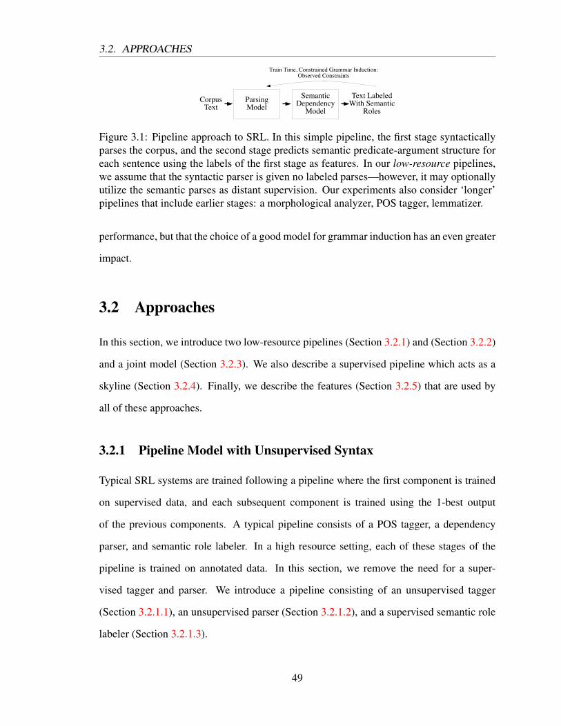
3.2. APPROACHES
ParsingModel
SemanticDependency
Model
CorpusText
Text LabeledWith Semantic
Roles
Train Time, Constrained Grammar Induction:Observed Constraints
Figure 3.1: Pipeline approach to SRL. In this simple pipeline, the first stage syntacticallyparses the corpus, and the second stage predicts semantic predicate-argument structure foreach sentence using the labels of the first stage as features. In our low-resource pipelines,we assume that the syntactic parser is given no labeled parses—however, it may optionallyutilize the semantic parses as distant supervision. Our experiments also consider ‘longer’pipelines that include earlier stages: a morphological analyzer, POS tagger, lemmatizer.
performance, but that the choice of a good model for grammar induction has an even greater
impact.
3.2 Approaches
In this section, we introduce two low-resource pipelines (Section 3.2.1) and (Section 3.2.2)
and a joint model (Section 3.2.3). We also describe a supervised pipeline which acts as a
skyline (Section 3.2.4). Finally, we describe the features (Section 3.2.5) that are used by
all of these approaches.
3.2.1 Pipeline Model with Unsupervised Syntax
Typical SRL systems are trained following a pipeline where the first component is trained
on supervised data, and each subsequent component is trained using the 1-best output
of the previous components. A typical pipeline consists of a POS tagger, a dependency
parser, and semantic role labeler. In a high resource setting, each of these stages of the
pipeline is trained on annotated data. In this section, we remove the need for a super-
vised tagger and parser. We introduce a pipeline consisting of an unsupervised tagger
(Section 3.2.1.1), an unsupervised parser (Section 3.2.1.2), and a supervised semantic role
labeler (Section 3.2.1.3).
49

3.2. APPROACHES
3.2.1.1 Brown Clusters
The first stage of our pipeline is an unsupervised tagger. Specifically, we use fully unsuper-
vised Brown clusters (Brown et al., 1992) in place of POS tags. Brown clusters have been
used to good effect for various NLP tasks such as named entity recognition (Miller et al.,
2004) and dependency parsing (Koo et al., 2008; Spitkovsky et al., 2011).
The clusters are formed by a greedy hierarchical clustering algorithm that finds an as-
signment of words to classes by maximizing the likelihood of the training data under a
latent-class bigram model. Each word type is assigned to a fine-grained cluster at a leaf of
the hierarchy of clusters. Each cluster can be uniquely identified by the path from the root
cluster to that leaf. Representing this path as a bit-string (with 1 indicating a left and 0 indi-
cating a right child) allows a simple coarsening of the clusters by truncating the bit-strings.
We train 1000 Brown clusters for each of the CoNLL-2009 languages on Wikipedia text.2
We restrict the vocabulary for each language to the 300,000 most common unigrams. The
open source implementation of Liang (2005) is used for training.
3.2.1.2 Unsupervised Grammar Induction
The second stage of the pipeline is an unsupervised syntactic parser. Here we perform
grammar induction by fully unsupervised Viterbi EM training of the Dependency Model
with Valence (DMV) (Klein and Manning, 2004), with uniform initialization of the model
parameters. We define the DMV such that it generates sequences of word classes: either
POS tags or Brown clusters as in Spitkovsky et al. (2011). The DMV is a simple generative
model for projective dependency trees. Children are generated recursively for each node.
Conditioned on the parent class, the direction (right or left), and the current valence (first
child or not), a coin is flipped to decide whether to generate another child; the distribution
over child classes is conditioned on only the parent class and direction. Spitkovsky et al.
2The Wikipedia text was tokenized for Polyglot (Al-Rfou’ et al., 2013): http://bit.ly/embeddings
50

3.2. APPROACHES
(2010a) show that Viterbi (hard) EM training of the DMV with simple uniform initialization
of the model parameters yields higher accuracy models than standard soft-EM training. In
Viterbi EM, the E-step finds the maximum likelihood corpus parse given the current model
parameters. The M-step then finds the maximum likelihood parameters given the corpus
parse. We utilize this approach to produce unsupervised syntactic features for the SRL task.
We follow Spitkovsky et al. (2010a) by starting with an E-step where the model pa-
rameters are uniformly initialized. Concurrently, Cohen and Smith (2010) observed that
starting with an M-step where the trees are chosen uniformly at random is also effective.
For the approach we take, ties must be broken randomly in the M-step parser. Otherwise,
undesirable bias may creep in during the first M-step.3 Again following Spitkovsky et al.
(2010a), we break ties within each chart cell. While this does not perfectly sample from the
set of maximum likelihood trees, we found it to be empirically effective and much simpler
than the algorithm required for breaking ties by sampling uniformly among trees.
3.2.1.3 Semantic Dependency Model
The third stage of the pipeline is a supervised SRL system that uses the 1-best output of
the previous two unsupervised stages (Brown clusters and DMV) as input. Semantic role
labeling can be cast as a structured prediction problem where the structure is a labeled
semantic dependency graph. We define a conditional random field (CRF) (Lafferty et al.,
2001) for this task. We describe the model here as a factor graph, as discussed in Sec-
tion 2.3.1. Because each word in a sentence may be in a semantic relationship with any
other word (including itself), a sentence of length n has n2 possible edges. We define a
single L+1-ary variable for each edge, whose value can be any of L semantic labels or a
special label indicating there is no predicate-argument relationship between the two words.
In this way, we jointly perform identification (determining whether a semantic relationship
exists) and classification (determining the semantic label). We include one unary factor for
3This was observed experimentally and resolved via personal correspondence with the first author ofSpitkovsky et al. (2010a).
51

3.2. APPROACHES
2 1 3 4
Ag.
Th.
Hl.
Juan_Carlos su abdica reino
Agent! Theme!Holder!
Figure 3.2: Example semantic roles for sentence and the corresponding variable assignmentof the factor graph for the semantic dependency model. A parse chart is overlaid to providea visual analogy with the parse chart in Figure 3.3. Each possible semantic edge has asingle L+1-ary variable. The variable corresponding to the edge from “abdica” to “reino”has value “Theme” (abbr. Th.) corresponding to the assigned semantic role shown belowthe sentence. The two variables with value “Agent” (abbr. Ag.) and “Holder” (abbr. HL)indicate that “Juan Carlos” fills two semantic roles for “abdica” and “reino” respectively.All other variables have value ∅ to indicate that they assign no semantic role.
each variable.
We optionally include additional variables that perform word sense disambiguation for
each predicate. Each has a unary factor and is completely disconnected from the semantic
edge (similar to Naradowsky et al. (2012a)). These variables range over all the predicate
senses observed in the training data for the lemma of that predicate. This effectively treats
the predicate sense prediction problem as a separate task. Including it allows us to compare
with prior work on the standard CoNLL-2009 benchmark.
3.2.2 Pipeline Model with Distantly-Supervised Syntax
Our second pipeline model is identical in form to the one presented in Section 3.2.1 ex-
cept that we replace the second stage: instead of unsupervised grammar induction as in
Section 3.2.1.2, we train the parser using the semantic roles as distant supervision.
52

3.2. APPROACHES
Juan_Carlos su abdica reino $
A0 A1 A0
Figure 3.3: Example of a pruned parse chart for constrained grammar induction. Thepruned edges are determined by the given semantic role labeling of the sentence. Eachchart cell (a square) contains two possible syntactic edges: a right edge (top triangle) anda left edge (bottom triangle). For example, the yellow edge would indicate that “abdica” isthe head of “reino”, whereas the black edge below it indicates that “reino” heads “abdica”.Only tokens filling at least one semantic role have edges to the possible parents pruned(black filled triangles). The chart cells with the word “reino” as a child correspond to theright diagonal of the chart (outlined in yellow)—all parents except for “abdica” have beenpruned since it is the only available semantic parent. The token “Juan Carlos” is the headof four edges (outlined in red), yet only two possible semantic parents—thus only the twocorresponding syntactic edges are not pruned. The English gloss is “Juan Carlos abdicateshis throne”, where $ indicates the special root node of the dependency parse. As usual, alledges with $ as a child are disallowed—along the left diagonal of the chart.
53
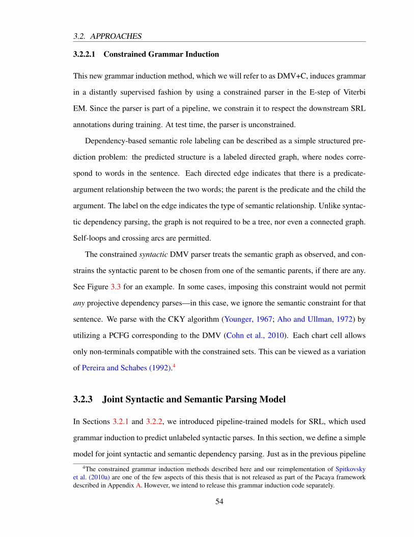
3.2. APPROACHES
3.2.2.1 Constrained Grammar Induction
This new grammar induction method, which we will refer to as DMV+C, induces grammar
in a distantly supervised fashion by using a constrained parser in the E-step of Viterbi
EM. Since the parser is part of a pipeline, we constrain it to respect the downstream SRL
annotations during training. At test time, the parser is unconstrained.
Dependency-based semantic role labeling can be described as a simple structured pre-
diction problem: the predicted structure is a labeled directed graph, where nodes corre-
spond to words in the sentence. Each directed edge indicates that there is a predicate-
argument relationship between the two words; the parent is the predicate and the child the
argument. The label on the edge indicates the type of semantic relationship. Unlike syntac-
tic dependency parsing, the graph is not required to be a tree, nor even a connected graph.
Self-loops and crossing arcs are permitted.
The constrained syntactic DMV parser treats the semantic graph as observed, and con-
strains the syntactic parent to be chosen from one of the semantic parents, if there are any.
See Figure 3.3 for an example. In some cases, imposing this constraint would not permit
any projective dependency parses—in this case, we ignore the semantic constraint for that
sentence. We parse with the CKY algorithm (Younger, 1967; Aho and Ullman, 1972) by
utilizing a PCFG corresponding to the DMV (Cohn et al., 2010). Each chart cell allows
only non-terminals compatible with the constrained sets. This can be viewed as a variation
of Pereira and Schabes (1992).4
3.2.3 Joint Syntactic and Semantic Parsing Model
In Sections 3.2.1 and 3.2.2, we introduced pipeline-trained models for SRL, which used
grammar induction to predict unlabeled syntactic parses. In this section, we define a simple
model for joint syntactic and semantic dependency parsing. Just as in the previous pipeline
4The constrained grammar induction methods described here and our reimplementation of Spitkovskyet al. (2010a) are one of the few aspects of this thesis that is not released as part of the Pacaya frameworkdescribed in Appendix A. However, we intend to release this grammar induction code separately.
54

3.2. APPROACHES
0 2 1 3 4 Juan_Carlos su abdica reino $
Y2,1
Z2,1
Y1,2
Z1,2
Y3,2
Z3,2
Y2,3
Z2,3 Y3,1
Z3,1
Y1,3
Z1,3
Y4,3
Z4,3
Y3,4
Z3,4 Y4,2
Z4,2
Y2,4
Z2,4 Y4,1
Z4,1
Y1,4
Z1,4
Z0,1
Z0,3
Z0,4
Z0,2
Figure 3.4: Factor graph for the joint syntactic/semantic dependency parsing model. Foreach of the O(n2) possible semantic edges between words i and j, there is a L+1-arysemantic role variable Yi,j (yellow). Each possible syntactic edge has a correspondingbinary variable Zi,j (blue). Variable pairs are connected by factors (black). The structuredPTREE factor (red) connects to the binary syntactic dependency variables and enforces thatthey form a projective tree. As in Figure 3.2, the special node $ is the syntactic root. Forthe possible syntactic edges from i → j and j → i, left/right within a chart cell of thisfigure corresponds to top/bottom in Figure 3.3.
methods, we use Brown clusters in place of POS tags (Section 3.2.1.1).
This model extends the CRF model in Section 3.2.1.3 to include the projective syntactic
dependency parse for a sentence. This is done by including an additional n2 binary vari-
ables that indicate whether or not a directed syntactic dependency edge exists between a
pair of words in the sentence. Unlike the semantic dependencies, these syntactic variables
must be coupled so that they produce a projective dependency parse; this requires an addi-
tional global constraint factor to ensure that this is the case (Smith and Eisner, 2008). The
constraint factor touches all n2 syntactic-edge variables, and multiplies in 1.0 if they form
a projective dependency parse, and 0.0 otherwise. We couple each syntactic edge variable
55

3.2. APPROACHES
to its semantic edge variable with a binary factor. Figure 3.4 shows the factor graph for this
joint model.
Note that our factor graph does not contain any loops, thereby permitting efficient
exact marginal inference. This is an instance of structured belief propagation (cf. Sec-
tion 2.3.3.4). We train our CRF models by maximizing conditional log-likelihood (cf.
Section 2.3.4.1) using stochastic gradient descent with an adaptive learning rate (AdaGrad)
(Duchi et al., 2011) over mini-batches of size 14 (cf. Section 2.4.2.4).
The unary and binary factors are defined with exponential family potentials. In the
next section, we consider binary features of the observations (the sentence and labels from
previous pipeline stages) which are conjoined with the state of the variables in the factor.
Discussion The factor graph we have presented here is almost identical to that of Narad-
owsky et al. (2012a). Our use of an L+1-ary semantic edge variable is in contrast to the
model of Naradowsky et al. (2012a), which used a more complex set of binary variables
and required a constraint factor permitting AT-MOST-ONE. Note that while these two ways
of defining the variables and factors are different, they encode the same model. Practically,
they differ in how we perform inference: in the Naradowsky et al. (2012a) model the fac-
tor graph has cycles and BP must be run to convergence. By contrast, our model requires
only a single iteration of BP with messages passed from leaves to root and back from root
to leaves (where the root is arbitrarily chosen). Both models thus permit efficient exact
inference.
3.2.4 Pipeline Model with Supervised Syntax (Skyline)
Though the focus of this chapter is on low-resource SRL, we also consider a high-resource
pipeline model in order to study the effectiveness of our models and features (described
below) in varying levels of supervision. For this supervised pipeline, we assume that we
are given either hand-annotated (i.e. gold) or automatically predicted lemmas, morphology,
56

3.2. APPROACHES
POS tags, and dependency parses. Given these annotations, we define features for the SRL-
only model described in Section 3.2.1.3.
3.2.5 Features for CRF Models
Our feature design stems from two key ideas. First, for SRL, it has been observed that
feature bigrams (the concatenation of simple features such as a predicate’s POS tag and
an argument’s word) are important for state-of-the-art performance (Zhao et al., 2009;
Bjorkelund et al., 2009). Second, for syntactic dependency parsing, combining Brown
cluster features with word forms or POS tags yields high accuracy even with little training
data (Koo et al., 2008).
We create binary indicator features for each model using feature templates. Our feature
template definitions combine those used by the top performing systems in the CoNLL-2009
Shared Task, Zhao et al. (2009) and Bjorkelund et al. (2009), and from features in syntactic
dependency parsing (McDonald et al., 2005; Koo et al., 2008). Though each base feature
comes from prior work, some of the feature combinations we construct are novel.
As is common in CRFs, we define our features as a conjunction of an indicator function
I for a fixed variable assignment yα with some observation function gα,k(x) of the input
sentence: fα,yα,k(yα,x) = I(yα = yα)gα,k(x). In the following subsections, we describe
the form of the observation functions gα,k that we consider in terms of a feature template
language.
3.2.5.1 Template Creation from Properties of Ordered Positions
The feature templates are defined using a simple template language comprised of three
types of functions:
1. Properties The property functions map a token position in a sentence to a string.
For example, given the position i, the function pos(i) returns the part-of-speech
(POS) tag for token i. We also allow these properties to be applied to a list of
57

3.2. APPROACHES
Property Possible values1 word(i) word form all word forms2 lc(i) lower case word form all lower-case forms3 chpre5(i) 5-char word form prefixes all 5-char form prefixes4 cap(i) capitalization True, False5 word800(i) top-800 word form top-800 word forms6 bc(i) brown cluster 000, 1100, 010110001, ...7 bc5(i) brown cluster, length 5 length 5 prefixes of bc8 lemma(i) lemma all word lemmas9 pos(i) POS tag NNP, CD, JJ, DT, ...10 m1(i), m2(i), . . . morphological features Gender, Case, Number, ...
(different across languages)11 deprel(i) dependency label SBJ, NMOD, LOC, ...12 dir(i) edge direction Up, Down
(a) Word and edge properties in SRL feature templates. For each property (left column) weshow examples of its possible values or a brief description of those values (right column).
τ(i) ρ(p, c)i, i-1, i+1 noFarChildren(i) linePath(p, c)
parent(i) rightNearSib(i) depPath(p, c)
allChildren(i) leftNearSib(i) depPath(p, lca(p, c))
rightNearChild(i) firstVSupp(i) depPath(c, lca(p, c))
rightFarChild(i) lastVSupp(i) depPath(lca(p, c), $)
leftNearChild(i) firstNSupp(i)
leftFarChild(i) lastNSupp(i)
(b) Word positions used in SRL feature templates. Based on current word posi-tion (i), positions related to current word i, possible parent, child (p, c), lowestcommon ancestor between parent/child (lca(p, c)), and syntactic root ($).
Template Possible valuesrelative-position before, after, ondistance Z+
continuity Z+
binned-distance > 2, 5, 10, 20, 30, or 40geneological-relationship parent, child, ancestor,
descendantpath-grams the NN went
(c) Additional standalone feature templates for SRL.
Table 3.1: Feature templates for semantic role labeling
58

3.2. APPROACHES
positions: pos([4, 8, 3]) returns a list of strings comprised of the POS tags of
words 4, 8, and 3 such as [VBN, NNP, NNP].
2. Position-modifiers The position modifier functions come in three forms. The first
form maps a single token position in a sentence to a new position: for example
parent(i) returns the syntactic head of token i. The second form maps a single
token to a list of positions: allChildren(i) returns the positions of all syntactic
dependents of token i. The third form maps a pair of positions to a list of positions:
depPath(p, c) returns the positions along the dependency path of between token
p and token c.
3. Orders We may wish to canonicalize a list of strings returned by a property applied
to a list of positions. For example pos(allChildren(i)) returns the list of POS
tags for the syntactic children of token i. The order function bag(l) returns the
concatenation of the sorted list of unique strings in list l. For example bag([VBN,
NNP, NNP]) = NNP VBN. In this way, we can obtain a canonically ordered set of
unique POS tags found among the syntactic children of token i using the feature
template bag(pos(allChildren(i))).
By composing these types of functions in different ways, we can obtain a wide variety of
templates.5 In the following paragraphs, we detail the properties (also listed in Table 3.1a),
positions and position-modifiers (also listed in Table 3.1b), and orders. We also consider a
few additional feature templates that do not fit within the property/position/order structure
above: these extra features are listed in Table 3.1c and described at the end of this sec-
tion. Note that this subsection only considers the base feature set. In the next subsection
(Section 3.2.6), we consider how these features can be composed by concatenating multi-
ple feature templates together—and more importantly how to select among the numerous
5Appendix A.2 describes the feature template language used in Pacaya which closely mirrors our featuredescriptions in this section.
59

3.2. APPROACHES
possibilities that result. Next, we consider how to define the observation function gα,k from
the feature templates we will define.
Observation Functions from Feature Templates Each feature template defines a map-
ping from a given sentence and position (or positions) to a string. From our example above,
bag(pos(allChildren(i))) returns a concatenation of POS tags. We assign an integer
index to each such string we observe during training. Suppose the integer k corresponds
to the string “NNP VBN”, then we would define g such that gα,k(x) = 1 if the template
bag(pos(allChildren(i))) returns “NNP VBN” and gα,k(x) = 0 otherwise. We define
g likewise for each integer k and its corresponding string / template. Note that each factor
α in the factor graph may use different observation functions. In practice, we use the same
observation-functions for each type of factor: e.g. all the unary factors for the role variables
have the same templates and separately all the unary factors for the sense variables have
the same templates.
The input positions to the feature templates are given by the variables that neighbor the
factor. See Figure 3.4 for an example factor graph. Each role variable Yp,c is defined for a
specific semantic dependency edge corresponding to a predicate token p and an argument
token c. Likewise, a link variable Zp,c has a (p, c) pair corresponding to the positions of the
parent and child for the syntactic edge. Each sense variable Sp defines a single position p
corresponding to the predicate.
Property Functions The properties include word form (word), lemma (lemma), POS
tag (pos), coarse (bc5) and fine-grained (bc) Brown cluster, and morphological features
(m1, m2, . . . ). We also include the lower-cased word (lc), the 5-character prefix if the word
is more than 5 characters (chpre5), whether the word is capitalized (cap), and the word
form only if it appears in the top 800 most frequent types (word800). Given a dependency
path, properties include the dependency relation of each word (deprel), and the direction
of the syntactic edge (dir). See Table 3.1a for example values that these properties can
60

3.2. APPROACHES
take.
Positions and Position-Modifier Functions Properties are extracted from word posi-
tions within the sentence. We define a set of unary operators τ(i) that generate positions
for a single word i which could be either the parent or child, and a set of binary operators
ρ(p, c). The position operators can return either a single position or a set of positions. Word
position operators are shown in Table 3.1b.
Single positions for a word i include the word to its left (i − 1) and right (i + 1),
its syntactic parent (parent), its leftmost farthest child (leftFarChild), its rightmost
nearest sibling (rightNearSib), etc. We also include the notion of verb and noun supports
(Zhao et al., 2009). A verb support (VSupp) position for i is a position above i in the
syntactic tree that has a verb POS, while a noun support (NSupp) has a noun POS.6 We
include two types of supports, corresponding to the support positions closest to i (first)
and closest to the root (last) respectively in the syntactic tree.
Sets of positions for a word i include children and the children (allChildren) without
the leftmost and rightmost included (noFarChildren). For a pair of positions (p, c),
we include the list of positions in their linear path (linePath) from left to right. Also
following previous work, we utilize four shortest dependency paths (Zhao et al., 2009)
with binary operator depPath: from parent to child, from parent to lca(p, c), from child
to lca(p, c), and from lca(p, c) to root—where lca(p, c) is the least-common-ancestor of
p and c in the syntactic parse.
Order Functions Following Zhao et al. (2009), properties from a set of positions can be
put together in three possible orders: as the given sequence (seq), as a sorted list of unique
strings (bag), and removing all duplicated neighbored strings (noDup).
6These features are informative only in our models that use POS tags.
61

3.2. APPROACHES
3.2.5.2 Additional Features
Additional templates we include are the relative position (relative-position) (Bjorkelund
et al., 2009), geneological relationship (geneological-relationship), distance (distance)
(Zhao et al., 2009), and binned distance (binned-distance) (Koo et al., 2008) be-
tween two words in the path. From Lluıs et al. (2013), we use 1, 2, 3-gram path features
of words/POS tags (path-grams), and the number of non-consecutive token pairs in a
predicate-argument path (continuity). Possible values these features can take are shown
in Table 3.1c.
3.2.6 Feature Selection
Constructing all feature templates (herein called template unigrams) and pairs of templates
(template bigrams) would yield an unwieldy number of features. We therefore include all
template unigrams, but only a subset of template bigrams. These are chosen to be the top
N template bigrams for a dataset and factor α according to an information gain measure
(Martins et al., 2011a):
IGα,m =∑
f∈Tm
∑
yα
p(f,yα) log2p(f,yα)
p(f)p(yα)(3.1)
where Tm is the mth feature template, f is a particular instantiation of that template, and
yα is an assignment to the variables in factor α. The probabilities are empirical estimates
computed from the training data. This is simply the mutual information of the feature
template instantiation with the variable assignment.
This filtering approach was treated as a simple baseline in Martins et al. (2011a) to
contrast with increasingly popular gradient-based regularization approaches. Unlike the
gradient-based approaches, this filtering approach easily scales to many features since we
can decompose the memory usage over feature templates.
As an additional speedup, we reduce the dimensionality of our feature space to 1 million
62

3.3. RELATED WORK
for each clique using a common trick referred to as feature hashing (Weinberger et al.,
2009): we map each feature instantiation to an integer using a hash function7 modulo the
desired dimensionality.
Example feature templates Table 3.2 shows the bigram feature templates that were se-
lected according to the information gain criterion on the English CoNLL-2009 data. The
selected templates highlight a key shortcoming of the approach: because the information
gain computation is independent for each feature, there is nothing to encourage diversity
among the selected features. As such, the top features are highly redundant. For exam-
ple, the first four templates conjoin word800(c) with either the word, lower-cased word,
5-character prefix of the word, or its lemma.
3.3 Related Work
Our work builds upon research in both semantic role labeling and unsupervised gram-
mar induction (Klein and Manning, 2004; Spitkovsky et al., 2010a). Previous related
approaches to semantic role labeling include joint classification of semantic arguments
(Toutanova et al., 2005; Johansson and Nugues, 2008), latent syntax induction (Boxwell
et al., 2011; Naradowsky et al., 2012a), and feature engineering for SRL (Zhao et al., 2009;
Bjorkelund et al., 2009).
High-resource SRL As discussed in the introduction, semantic role labeling is tradition-
ally approached by first identifying syntactic features of the sentence and then predicting
predicates and their arguments. These often use a pipeline of classifiers for predicate disam-
biguation, argument identification, and argument classification (Gildea and Jurafsky, 2000;
Gildea and Jurafsky, 2002; Surdeanu et al., 2008). Such pipeline approaches rely heavily
on the accuracy of the syntactic parser (Gildea and Palmer, 2002; Punyakanok et al., 2005).
7To reduce hash collisions, we use MurmurHash v3 https://code.google.com/p/smhasher.
63

3.3. RELATED WORK
Bigram Template IGa,m
word800(c) + word(p) 2.841077word800(c) + lc(p) 2.840362word800(c) + chpre5(p) 2.822854word800(c) + lemma(p) 2.815270word(c) + word(p) 2.738279lemma(c) + word(p) 2.735499word(c) + lc(p) 2.735469lc(c) + lc(p) 2.735363chpre5(c) + lc(p) 2.733696chpre5(c) + word(p) 2.733115lemma(c) + lc(p) 2.732447lc(c) + word(p) 2.731534bc(c) + lc(p) 2.726672bc(c) + word(p) 2.725611word(c) + chpre5(p) 2.725222lemma(c) + chpre5(p) 2.720818lc(c) + chpre5(p) 2.719960word(c) + lemma(p) 2.719056chpre5(c) + chpre5(p) 2.716669chpre5(c) + lemma(p) 2.713464lc(c) + lemma(p) 2.712567lemma(c) + lemma(p) 2.711402bc(c) + chpre5(p) 2.709945word800(c) + word800(p) 2.707732seq(pos(linePath(p, c))) + word(p) 2.704583seq(pos(linePath(p, c))) + lemma(p) 2.702469seq(pos(linePath(p, c))) + lc(p) 2.701657bc(c) + lemma(p) 2.695978word800(c) + bc(p) 2.695099seq(pos(linePath(p, c))) + chpre5(p) 2.689965seq(deprel(linePath(p, c))) + word(p) 2.685279seq(deprel(linePath(p, c))) + lc(p) 2.683995
Table 3.2: Top 32 bigram feature templates ranked by information gain (IGa,m) on seman-tic argument classification the first 1000 sentences of the English CoNLL-2009 data. +indicates the conjoining of two templates. See Section 3.2.5 for a description of the featuretemplate language used here. p is the position of the predicate and c the position of theargument.
64

3.3. RELATED WORK
This decomposition prohibits the parser from utilizing the labels from the end task.
Toutanova et al. (2005) introduced one of the first joint approaches for SRL and demon-
strated that a model that scores the full predicate-argument structure of a parse tree could
lead to significant error reduction over independent classifiers for each predicate-argument
relation.
Johansson and Nugues (2008) and Lluıs et al. (2013) extend this idea by coupling pre-
dictions of a dependency parser with predictions from a semantic role labeler. In the model
from Johansson and Nugues (2008), the outputs from an SRL pipeline are reranked based
on the full predicate-argument structure that they form. The candidate set of syntactic-
semantic structures is reranked using the probability of the syntactic tree and semantic
structure. Lluıs et al. (2013) use a joint arc-factored model that predicts full syntactic paths
along with predicate-argument structures via dual decomposition.
Low-resource SRL Boxwell et al. (2011) and Naradowsky et al. (2012a) observe that
syntax may be treated as latent when a treebank is not available. Boxwell et al. (2011)
describe a method for training a semantic role labeler by extracting features from a packed
CCG parse chart, where the parse weights are given by a simple ruleset. Naradowsky et al.
(2012a) marginalize over latent syntactic dependency parses.
Both Boxwell et al. (2011) and Naradowsky et al. (2012a) suggest methods for SRL
without supervised syntax, however, their features come largely from supervised resources.
Even in their lowest resource setting, Boxwell et al. (2011) require an oracle CCG tag
dictionary extracted from a treebank. Naradowsky et al. (2012a) limit their exploration to a
small set of basic features, and included high-resource supervision in the form of lemmas,
POS tags, and morphology available from the CoNLL 2009 data.
There has not yet been a comparison of techniques for SRL that do not rely on a syn-
tactic treebank, and no exploration of probabilistic models for unsupervised grammar in-
duction within an SRL pipeline that we have been able to find.
65

3.4. EXPERIMENTAL SETUP
Grammar Induction Related work for the unsupervised learning of dependency struc-
tures separately from semantic roles primarily comes from Klein and Manning (2004), who
introduced the Dependency Model with Valence (DMV). This is a robust generative model
that uses a head-outward process over word classes, where heads generate arguments.
Grammar induction work has further demonstrated that distant supervision in the form
of ACE-style relations (Naseem and Barzilay, 2011) or HTML markup (Spitkovsky et al.,
2010b) can lead to considerable gains. Recent work in fully unsupervised dependency
parsing has supplanted these methods with even higher accuracies (Spitkovsky et al., 2013)
by arranging optimizers into networks that suggest informed restarts based on previously
identified local optima. We do not reimplement these approaches within the SRL pipeline
here, but provide comparison of these methods against our grammar induction approach in
isolation in Section 3.5.4.
Feature Templates for SRL In both pipeline and joint models, we use features adapted
from state-of-the-art approaches to SRL (Section 3.2.5). This includes Zhao et al. (2009)
features, who use feature templates from combinations of word properties, syntactic posi-
tions including head and children, and semantic properties; and features from Bjorkelund et
al. (2009), who utilize features on syntactic siblings and the dependency path concatenated
with the direction of each edge.
3.4 Experimental Setup
3.4.1 Data
The CoNLL-2009 Shared Task (Hajic et al., 2009) dataset contains POS tags, lemmas,
morphological features, syntactic dependencies, predicate senses, and semantic roles an-
notations for 7 languages: Catalan, Chinese, Czech, English, German, Japanese,8 Spanish.
8We do not report results on Japanese as that data was only made freely available to researchers thatcompeted in CoNLL 2009.
66

3.4. EXPERIMENTAL SETUP
The CoNLL-2005 and -2008 Shared Task datasets provide English SRL annotation, and
for cross-dataset comparability we consider only verbal predicates. To compare with prior
approaches that use semantic supervision for grammar induction, we utilize Section 23 of
the WSJ portion of the Penn Treebank (Marcus et al., 1993).
The CoNLL-2005, CoNLL-2008, and English CoNLL-2009 datasets share the same
underlying sentences from the Penn Treebank. However, the exact set of sentences included
in the respective shared tasks differ slightly. The argument annotations in CoNLL-2005
are over spans, whereas the heads of arguments are annotated in CoNLL-2008 and -2009.
These details are further described in Section 3.5.2.
The standard evaluation for CoNLL-2009 includes sense prediction as well as argument
identification and classification. While we view sense prediction as somewhat tangential to
our discussion of SRL, we include it in some of the evaluation metrics in order to compare
to prior work.
3.4.2 Feature Template Sets
We consider two sets of features based on the information gain feature selection criterion.
Our primary feature set, IGC , consists of 127 template unigrams. Note that this is not every
possible feature template describable by our feature template language, but rather a subset
that emphasizes coarse word properties (i.e., properties 7, 9, and 11 in Table 3.1a). We also
explore the 31 template unigrams9 described by Bjorkelund et al. (2009), here referred to
as IGB. Each of IGC and IGB also include 32 template bigrams selected by information
gain on 1000 sentences—we select a different set of template bigrams for each dataset.
We compare against the language-specific feature sets detailed in the literature on high-
resource top-performing SRL systems: From Bjorkelund et al. (2009), these are feature
sets for German, English, Spanish and Chinese, obtained by weeks of forward selection
9Because we do not include a binary factor between predicate sense and semantic role, we do not includesense as a feature for argument prediction.
67

3.5. RESULTS
(Bde,en,es,zh); and from Zhao et al. (2009), these are features for Catalan Zca.10
3.5 Results
We are interested in the effects of varied supervision using pipeline and joint training for
SRL. To compare to prior work (i.e., submissions to the CoNLL-2009 Shared Task), we
also consider the joint task of semantic role labeling and predicate sense disambiguation.
Our experiments are subtractive, beginning with all supervision available and then succes-
sively removing (a) dependency syntax, (b) morphological features, (c) POS tags, and (d)
lemmas. Dependency syntax is the most expensive and difficult to obtain of these various
forms of supervision. We explore the importance of both the labels and structure, and what
quantity of supervision is useful.
3.5.1 CoNLL-2009: High-resource SRL
We first compare our models trained as a pipeline, using all available supervision (syntax,
morphology, POS tags, lemmas) from the CoNLL-2009 data.
Gold Syntax Table 3.3 shows the results of our model with gold syntax and a richer fea-
ture set than that of Naradowsky et al. (2012a), which only looked at whether a syntactic
dependency edge was present. Table 3.6(a) contains the full per-language results for the av-
erages shown in Table 3.3 as well as additional feature template settings (Zca, Bde,en,es,zh).
Recall an important advantage of the pipeline trained model: the features can consider any
part of the syntax (e.g., arbitrary subtrees), whereas the joint model is limited to those fea-
tures over which it can efficiently marginalize (e.g., short dependency paths). This holds
true even in the pipeline setting where no syntactic supervision is available. The contrast
of our pipeline with rich features on gold syntax (84.98 Avg. F1) vs. Naradowsky et al.
10This covers all CoNLL languages but Czech, where feature sets were not made publicly available ineither work. In Czech, we disallowed template bigrams involving path-grams.
68

3.5. RESULTS
SRL Approach Feature Set Avg. F1Pipeline IGC 84.98Pipeline IGB 84.74Naradowsky et al. (2012a) 72.73
Table 3.3: Test F1 of supervised SRL and sense disambiguation with gold (oracle) syntaxaveraged over the CoNLL-2009 languages. See Table 3.6(a) for per-language results.
(2012a) which uses a limited feature set on gold syntax (72.73 Avg. F1) demonstrates the
importance of rich features in the high-resource setting: without such features performance
suffers (a 12.25 drop in Avg. F1). Including such features in a joint model requires approx-
imate inference such as BP or dual decomposition (cf. Lluıs et al. (2013)). In this chapter,
we have restricted our attention to joint models for which exact inference is possible (i.e.
without rich features), yet we will observe that even with a limited feature set, the joint
model can outperform a feature-rich model in the low-resource setting.
Supervised Syntax Table 3.4 uses predicted (not gold) syntax and contrasts our high-
resource results for the task of SRL and sense disambiguation with the top systems in the
CoNLL-2009 Shared Task, giving further insight into the performance of the simple infor-
mation gain feature selection technique. With supervised syntax, the simple information
gain feature selection technique (Section 3.2.6) applied to a large set of 127 template un-
igrams IGC performs admirably (78.03 Avg. F1), but still lags behind the state-of-the-art
from Bjorkelund et al. (2009) (81.55 Avg. F1). Using only a reduced set of 32 template
unigrams IGB for feature selection, we see a drop in performance (75.68 Avg. F1).
Table 3.6(b) presents the per-language results corresponding to the averages in Table 3.4
as well as results with language-specific feature sets from prior work (Zca, Bde,en,es,zh).
Here we can contrast two feature selection techniques: The original Bjorkelund features
(Bde,en,es,zh) were selected by a computationally intensive search through possible template
bigrams: each bigram was added to the model and kept only if the F1 score of the high-
resource model improved on development data. Our feature set IGB began with the same
set of template unigrams, but selected the template bigrams by a (comparatively simple)
69
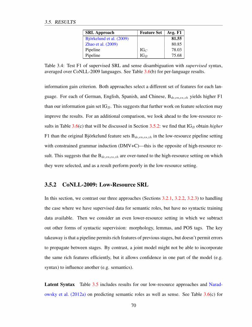
3.5. RESULTS
SRL Approach Feature Set Avg. F1Bjorkelund et al. (2009) 81.55Zhao et al. (2009) 80.85Pipeline IGC 78.03Pipeline IGB 75.68
Table 3.4: Test F1 of supervised SRL and sense disambiguation with supervised syntax,averaged over CoNLL-2009 languages. See Table 3.6(b) for per-language results.
information gain criterion. Both approaches select a different set of features for each lan-
guage. For each of German, English, Spanish, and Chinese, Bde,en,es,zh yields higher F1
than our information gain set IGB. This suggests that further work on feature selection may
improve the results. For an additional comparison, we look ahead to the low-resource re-
sults in Table 3.6(c) that will be discussed in Section 3.5.2: we find that IGB obtain higher
F1 than the original Bjorkelund feature sets Bde,en,es,zh in the low-resource pipeline setting
with constrained grammar induction (DMV+C)—this is the opposite of high-resource re-
sult. This suggests that the Bde,en,es,zh are over-tuned to the high-resource setting on which
they were selected, and as a result perform poorly in the low-resource setting.
3.5.2 CoNLL-2009: Low-Resource SRL
In this section, we contrast our three approaches (Sections 3.2.1, 3.2.2, 3.2.3) to handling
the case where we have supervised data for semantic roles, but have no syntactic training
data available. Then we consider an even lower-resource setting in which we subtract
out other forms of syntactic supervision: morphology, lemmas, and POS tags. The key
takeaway is that a pipeline permits rich features of previous stages, but doesn’t permit errors
to propagate between stages. By contrast, a joint model might not be able to incorporate
the same rich features efficiently, but it allows confidence in one part of the model (e.g.
syntax) to influence another (e.g. semantics).
Latent Syntax Table 3.5 includes results for our low-resource approaches and Narad-
owsky et al. (2012a) on predicting semantic roles as well as sense. See Table 3.6(c) for
70

3.5. RESULTS
SRL Approach Feature Set Dep. Parser Avg. F1Joint IGC Marginalized 72.48Joint IGB Marginalized 72.40Naradowsky et al. (2012a) Marginalized 71.27Pipeline IGC DMV+C (bc) 70.08Pipeline IGC DMV (bc) 69.26Pipeline IGB DMV (bc) 66.81Pipeline IGB DMV+C (bc) 65.61
Table 3.5: Test F1 of supervised SRL and sense disambiguation with no supervision forsyntax, averaged over CoNLL-2009 languages. See Table 3.6(c) for per-language results.
per-language results and additional features not shown in Table 3.5. In the low-resource
setting of the CoNLL-2009 Shared task without syntactic supervision, our joint model
(Joint) with marginalized syntax obtains state-of-the-art results with features IGC described
in Section 3.4.2. This model outperforms prior work (Naradowsky et al., 2012a) and our
pipeline model (Pipeline) with constrained (DMV+C) and unconstrained grammar induc-
tion (DMV) trained on brown clusters (bc).
These results begin to answer a key research question in this work: The joint models
outperform the pipeline models in the low-resource setting. This holds even when using the
same feature selection process. Further, the best-performing low-resource features found
in this work are those based on coarse feature templates and selected by information gain.
Templates for these features generalize well to the high-resource setting. However, analysis
of the induced grammars in the pipeline setting suggests that the book is not closed on the
issue. We return to this in Section 3.5.4.
Training and decoding times for the pipeline and joint methods are similar as computa-
tion time tends to be dominated by feature extraction.
Subtractive Study In our subsequent experiments, we study the effectiveness of our
models as the available supervision is decreased. We incrementally remove dependency
syntax, morphological features, POS tags, then lemmas. For these experiments, we utilize
the coarse-grained feature set (IGC), which includes Brown clusters.
71

3.5. RESULTS
(a)
(b)
(c)
SRL
App
roac
hFe
atur
eSe
tD
ep.P
arse
rAv
g.ca
csde
enes
zhPi
pelin
eIG
CG
old
84.9
884
.97
87.6
579
.14
86.5
484
.22
87.3
5Pi
pelin
eZca
Gol
d*8
6.49
86.4
9—
——
——
Pipe
line
IGB
Gol
d84
.74
85.1
586
.64
79.5
085
.77
84.4
086
.95
Pipe
line
Bde,en,es,zh
Gol
d*8
3.80
——
77.0
685
.62
85.4
987
.03
Nar
adow
sky
etal
.(20
12a)
Gol
d72
.73
69.5
974
.84
66.4
978
.55
68.9
377
.97
Bjo
rkel
und
etal
.(20
09)
Supe
rvis
ed81
.55
80.0
185
.41
79.7
185
.63
79.9
178
.60
Zha
oet
al.(
2009
)Su
perv
ised
80.8
580
.32
85.1
975
.99
85.4
480
.46
77.7
2Pi
pelin
eIG
CSu
perv
ised
78.0
376
.24
83.3
474
.19
81.9
676
.12
76.3
5Pi
pelin
eZca
Supe
rvis
ed*7
7.62
77.6
2—
——
——
Pipe
line
Bde,en,es,zh
Supe
rvis
ed*7
6.49
——
72.1
781
.15
76.6
575
.99
Pipe
line
IGB
Supe
rvis
ed75
.68
74.5
981
.61
69.0
878
.86
74.5
175
.44
Join
tIG
CM
argi
naliz
ed72
.48
71.3
581
.03
65.1
576
.16
71.0
370
.14
Join
tIG
BM
argi
naliz
ed72
.40
71.5
580
.04
64.8
075
.57
71.2
171
.21
Nar
adow
sky
etal
.(20
12a)
Mar
gina
lized
71.2
767
.99
73.1
667
.26
76.1
266
.74
76.3
2Jo
int
Zca
Mar
gina
lized
*70.
9870
.98
——
——
—Pi
pelin
eIG
CD
MV
+C(b
c)70
.08
68.2
179
.63
62.2
573
.81
68.7
367
.86
Pipe
line
Zca
DM
V+C
(bc)
*69.
6769
.67
——
——
—Pi
pelin
eIG
CD
MV
(bc)
69.2
668
.04
79.5
858
.47
74.7
868
.36
66.3
5Pi
pelin
eIG
BD
MV
(bc)
66.8
163
.31
77.3
859
.91
72.0
265
.96
62.2
8Jo
int
Bde,en,es,zh
Mar
gina
lized
*65.
63—
—60
.05
71.0
665
.34
66.0
7Pi
pelin
eIG
BD
MV
+C(b
c)65
.61
61.8
977
.48
58.9
769
.11
63.3
162
.92
Pipe
line
Bde,en,es,zh
DM
V+C
(bc)
*63.
06—
—57
.75
68.3
263
.70
62.4
5
Tabl
e3.
6:Te
stF1
for
SRL
and
sens
edi
sam
bigu
atio
non
CoN
LL’
09in
high
-res
ourc
ean
dlo
w-r
esou
rce
setti
ngs:
we
stud
y(a
)go
ldsy
ntax
,(b)
supe
rvis
edsy
ntax
,and
(c)
unsu
perv
ised
synt
ax.
Res
ults
are
rank
edby
F1w
ithbo
ldnu
mbe
rsin
dica
ting
the
best
F1fo
ra
lang
uage
and
leve
lofs
uper
visi
on.
*Ind
icat
espa
rtia
lave
rage
sfo
rthe
lang
uage
-spe
cific
feat
ure
sets
(Zca
and
Bde,en,es,zh
),fo
rwhi
chw
esh
owre
sults
only
onth
ela
ngua
ges
forw
hich
the
sets
wer
epu
blic
lyav
aila
ble.
72

3.5. RESULTS
Rem #FT ca de es
– 127+32 74.46 72.62 74.23Dep 40+32 67.43 64.24 67.18Mor 30+32 67.84 59.78 66.94POS 23+32 64.40 54.68 62.71Lem 21+32 64.85 54.89 63.80
Table 3.7: Subtractive experiments. Each row contains the F1 for SRL only (without sensedisambiguation) where the supervision type of that row and all above it have been removed.Removed supervision types (Rem) are: syntactic dependencies (Dep), morphology (Mor),POS tags (POS), and lemmas (Lem). #FT indicates the number of feature templates used(unigrams+bigrams).
Across languages, we find the largest drop in F1 when we remove POS tags; and we
find a gain in F1 when we remove lemmas. This indicates that lemmas, which are a high-
resource annotation, may not provide a significant benefit for this task. The effect of remov-
ing morphological features is different across languages, with little change in performance
for Catalan and Spanish, but a drop in performance for German. This may reflect a dif-
ference between the languages, or may reflect the difference between the annotation of the
languages: both the Catalan and Spanish data originated from the Ancora project,11 while
the German data came from another source.
Figure 3.5 contains the learning curve for SRL supervision in our lowest resource set-
ting for two example languages, Catalan and German. This shows how F1 of SRL changes
as we adjust the number of training examples. We find that the joint training approach to
grammar induction yields consistently higher SRL performance than its distantly super-
vised counterpart.
3.5.3 CoNLL-2008, -2005 without a Treebank
In this section, we return to the “no syntax” setting of the previous section. We do so in
order to contrast our dependency-based SRL models with that of a state-of-the-art span-
based SRL model. This provides the first such comparison in the low-resource setting.11http://clic.ub.edu/corpus/ancora
73

3.5. RESULTS
20
30
40
50
60
70
0 20000 40000 60000Number of Training Sentences
Labe
led
F1Language / Dependency Parser
Catalan / MarginalizedCatalan / DMV+CGerman / MarginalizedGerman / DMV+C
Figure 3.5: Learning curve for semantic dependency supervision in Catalan and German.F1 of SRL only (without sense disambiguation) shown as the number of training sentencesis increased.
traintest 2008
heads2005spans
2005spans
(oracletree)
✓□ PRY’08
2005
span
s 84.32 79.44□ B’11 (tdc) — 71.5□ B’11 (td) — 65.0✓□ JN’08
2008
head
s 85.93 79.90□ Joint, IGC 72.9 35.0 72.0□ Joint, IGB 67.3 37.8 67.1
Table 3.8: F1 for SRL approaches (without sense disambiguation) in matched and mis-matched train/test settings for CoNLL 2005 span and 2008 head supervision. We contrastlow-resource (□) and high-resource settings (✓□), where the latter uses a treebank. SeeSection 3.5.2 for caveats to this comparison.
We contrast our approach with that of Boxwell et al. (2011), who evaluate on semantic
argument identification and classification in isolation—that is, they do not include predicate
sense disambiguation, as is done in the CoNLL-2009 Shared Task benchmark. They report
results on Prop-CCGbank (Boxwell and White, 2008), which uses the same training/testing
splits as the CoNLL-2005 Shared Task. Their results are therefore loosely12 comparable to
results on the CoNLL-2005 dataset.12The comparison is imperfect for two reasons: first, the CCGBank contains only 99.44% of the original
PTB sentences (Hockenmaier and Steedman, 2007); second, because PropBank was annotated over CFGs,after converting to CCG only 99.977% of the argument spans were exact matches (Boxwell and White, 2008).However, this comparison was adopted by Boxwell et al. (2011), so we use it here.
74

3.5. RESULTS
There is an additional complication in comparing SRL approaches directly: The CoNLL-
2005 dataset defines arguments as spans instead of heads, which runs counter to our head-
based syntactic representation. This creates a mismatched train/test scenario: we must
train our model to predict argument heads, but then test on our model’s ability to predict
argument spans.13 We therefore train our models on the CoNLL-2008 argument heads,14
and post-process and convert from heads to spans using the conversion algorithm available
from Johansson and Nugues (2008).15 The heads are either from an MBR tree or an oracle
tree. This gives Boxwell et al. (2011) the advantage, since our syntactic dependency parses
are optimized to pick out semantic argument heads, not spans.
Table 3.8 presents our results. Boxwell et al. (2011) (B’11) uses additional supervision
in the form of a CCG tag dictionary derived from supervised data with (tdc) and without
(tc) a cutoff. Our model does very poorly on the ’05 span-based evaluation because the
constituent bracketing of the marginalized trees are inaccurate. This is elucidated by instead
evaluating on the oracle spans, where our F1 scores are higher than Boxwell et al. (2011).
We also contrast with relevant high-resource methods with span/head conversions from
Johansson and Nugues (2008): Punyakanok et al. (2008) (PRY’08) and Johansson and
Nugues (2008) (JN’08).
3.5.4 Analysis of Grammar Induction
Table 3.9 shows grammar induction accuracy in low-resource settings. We find that the
gap between the supervised parser and the unsupervised methods is quite large, despite the
reasonable accuracy both methods achieve for the SRL end task. This suggests that refining
the low-resource grammar induction methods may lead to gains in SRL.
13We were unable to obtain the system output of Boxwell et al. (2011) in order to convert their spans todependencies and evaluate the other mismatched train/test setting.
14CoNLL-2005, -2008, and -2009 were derived from PropBank and share the same source text; -2008 and-2009 use argument heads.
15Specifically, we use their Algorithm 2, which produces the span dominated by each argument, with spe-cial handling of the case when the argument head dominates that of the predicate. Also following Johanssonand Nugues (2008), we recover the ’05 sentences missing from the ’08 evaluation set.
75

3.6. SUMMARY
Dependency Parser Avg. ca cs de en es zhSupervised* 87.1 89.4 85.3 89.6 88.4 89.2 80.7DMV (pos) 30.2 45.3 22.7 20.9 32.9 41.9 17.2DMV (bc) 22.1 18.8 32.8 19.6 22.4 20.5 18.6DMV+C (pos) 37.5 50.2 34.9 21.5 36.9 49.8 32.0DMV+C (bc) 40.2 46.3 37.5 28.7 40.6 50.4 37.5Marginal, IGC 43.8 50.3 45.8 27.2 44.2 46.3 48.5Marginal, IGB 50.2 52.4 43.4 41.3 52.6 55.2 56.2
Table 3.9: Unlabeled directed dependency accuracy on CoNLL’09 test set in low-resourcesettings. DMV models are trained on either POS tags (pos) or Brown clusters (bc). *Indicatesthe supervised parser outputs provided by the CoNLL’09 Shared Task.
The marginalized grammars best the DMV grammar induction method; however, this
difference is less pronounced when the DMV is constrained using SRL labels as distant
supervision. This could indicate that a better model for grammar induction would result
in better performance for SRL. We therefore turn to an analysis of other approaches to
grammar induction in Table 3.10, evaluated on the Penn Treebank. We contrast with meth-
ods using distant supervision (Naseem and Barzilay, 2011; Spitkovsky et al., 2010b) and
fully unsupervised dependency parsing (Spitkovsky et al., 2013). Following prior work, we
exclude punctuation from evaluation and convert the constituency trees to dependencies.16
The approach from Spitkovsky et al. (2013) (SAJ’13) outperforms all other approaches,
including our marginalized settings. We therefore may be able to achieve further gains in
the pipeline model by considering better models of latent syntax, or better search techniques
that break out of local optima. Similarly, improving the nonconvex optimization of our
latent-variable CRF (Marginalized) may offer further gains.
3.6 Summary
We have compared various approaches for low-resource semantic role labeling at the state-
of-the-art level. We find that we can outperform prior work in the low-resource setting by
16Naseem and Barzilay (2011) and our results use the Penn converter (Pierre and Heiki-Jaan, 2007).Spitkovsky et al. (2010; 2013) use Collins (1999) head percolation rules.
76

3.6. SUMMARY
WSJ∞ DistantSupervision
SAJM’10 44.8 noneSAJ’13 64.4 noneSJA’10 50.4 HTMLNB’11 59.4 ACE05DMV (bc) 24.8 noneDMV+C (bc) 44.8 SRLMarginalized, IGC 48.8 SRLMarginalized, IGB 58.9 SRL
Table 3.10: Comparison of grammar induction approaches on the Penn Treebank. Wecontrast the DMV trained with Viterbi EM+uniform initialization (DMV), our constrainedDMV (DMV+C), and our model’s MBR decoding of latent syntax (Marginalized) withother recent work: Spitkovsky et al. (2010a) (SAJM’10), Spitkovsky et al. (2010b)(SJA’10), Naseem and Barzilay (2011) (NB’11), and the CS model of Spitkovsky et al.(2013) (SAJ’13).
coupling the selection of feature templates based on information gain with a joint model
that marginalizes over latent syntax.
We utilize unlabeled data in both generative and discriminative models for dependency
syntax and in generative word clustering. Our discriminative joint models treat latent syn-
tax as a structured-feature to be optimized for the end-task of SRL, while our other gram-
mar induction techniques optimize for unlabeled data likelihood—optionally with distant
supervision. We observe that careful use of these unlabeled data resources can improve
performance on the end task.
Our subtractive experiments suggest that lemma annotations, a high-resource annota-
tion, may not provide a large benefit for SRL. Our grammar induction analysis indicates
that relatively low accuracy can still result in reasonable SRL predictions; still, the models
do not perform at the level of those that use supervised syntax. In future work, we hope to
explore how well the pipeline models in particular improve when we apply higher accuracy
unsupervised grammar induction techniques.
77

Chapter 4
Neural and Log-linear Factors
Over a decade of research has been spent carefully crafting features by hand for the task
of relation extraction (Zelenko et al., 2003; Culotta and Sorensen, 2004; Bunescu and
Mooney, 2005; Jiang and Zhai, 2007; Sun et al., 2011; Plank and Moschitti, 2013; Nguyen
and Grishman, 2014). Yet, there has been much recent effort in attempting to show that
these sorts of features can be learned automatically with neural networks. One of the con-
veniences of the proposed framework of this thesis is that these neural networks can easily
be incorporated. However, for areas in which decades of research have been spent care-
fully crafting features by hand, does the application-blind machinery of neural networks
still have something to offer?
In this chapter,1 we pose this question and study it experimentally. We augment a
baseline relation extraction system consisting of handcrafted features with a state-of-the-
art neural network architecture—this hybrid model is the focus of this chapter. Our goal
is to demonstrate the complementarity of the two submodels. There have been increas-
ingly many results that suggest handcrafted features are complementary to those learned
by (current) neural networks; see for example Socher et al. (2012). Similar results in rela-
tion extraction (Hashimoto et al., 2015; Liu et al., 2015) and constituency parsing (Durrett
and Klein, 2015) appeared while this thesis was in preparation. However, we believe that1A previous version of this work was presented in Gormley et al. (2015b).
78

4.1. INTRODUCTION
Class Sentence Snippet(a) ART(M1,M2) [M1 A man ] driving what appeared to be [M2 a taxicab ](b) PART-WHOLE(M1,M2) direction of [M1 the southern suburbs ] of [M2 Baghdad ](c) PHYSICAL(M2,M1) in [M1 the united states ], [M2 284 people ] died
Table 4.1: Examples from ACE 2005. In (a), the word “driving” is a strong indicator of therelation ART between M1 and M2. A feature that depends on the embedding for this con-text word could generalize to other lexical indicators of the same relation (e.g. “operating”)that don’t appear with ART during training. But lexical information alone is insufficient;relation extraction requires the identification of lexical roles: where a word appears struc-turally in the sentence. In (b), the word “of” between “suburbs” and “Baghdad” suggeststhat the first entity is part of the second, yet the earlier occurrence after “direction” is ofno significance to the relation. Even finer information can be expressed by a word’s roleon the dependency path between entities. In (c), we can distinguish the word “died” fromother irrelevant words that don’t appear between the entities.
ours is a particularly salient testing ground for the question at hand since we start with a
neural network which itself is infused with carefully constructed real-world knowledge of
the domain.
This chapter serves a secondary goal: to demonstrate the ease with which neural net-
works fit into our framework. Our full hybrid model provides for one of the simplest
examples of training in our framework—in the case where inference (as in the previous
chapter) makes no approximations. We reserve the case of approximate inference for the
final two chapters.
4.1 Introduction
Two common NLP feature types are lexical properties of words and unlexicalized linguis-
tic/structural interactions between words. Prior work on relation extraction has extensively
studied how to design such features by combining discrete lexical properties (e.g. the iden-
tity of a word, its lemma, its morphological features) with aspects of a word’s linguistic
context (e.g. whether it lies between two entities or on a dependency path between them).
While these help learning, they make generalization to unseen words difficult. An alter-
79

4.1. INTRODUCTION
native approach to capturing lexical information relies on continuous word embeddings.2
Embedding features have improved many tasks, including NER, chunking, dependency
parsing, semantic role labeling, and relation extraction (Miller et al., 2004; Turian et al.,
2010; Koo et al., 2008; Roth and Woodsend, 2014; Sun et al., 2011; Plank and Moschitti,
2013; Nguyen and Grishman, 2014). Embeddings can capture lexical information, but
alone they are insufficient: in state-of-the-art systems, they are used alongside features of
the broader linguistic context.
In this chapter, we introduce a hybrid log-linear and neural network model for relation
extraction, a task in which contextual feature construction plays a major role in generalizing
to unseen data. Our baseline log-linear model directly uses handcrafted lexicalized features.
The compositional model combines unlexicalized linguistic context and word embeddings.
We also show that this hybrid model is a (very simple) factor graph comprised of a single
variable and two factors: one factor has the standard exponential family form (i.e. the
log-linear model) and the other is a less-traditional factor (i.e. the neural network model).
The compositional model is called the Feature-rich Compositional Embedding Model
(FCM) and was introduced in Gormley et al. (2015b). FCM allows for the composition of
embeddings with arbitrary linguistic structure, as expressed by hand crafted features. In
the following sections, we describe the model starting with a precise construction of com-
positional embeddings using word embeddings in conjunction with unlexicalized features.
Various feature sets used in prior work (Turian et al., 2010; Nguyen and Grishman, 2014;
Hermann et al., 2014; Roth and Woodsend, 2014) are captured as special cases of this con-
struction. Adding these compositional embeddings directly to a standard log-linear model
yields a special case of the full FCM model. Treating the word embeddings as parameters
gives rise to the powerful, efficient, and easy-to-implement log-bilinear model. The model
capitalizes on arbitrary types of linguistic annotations by better utilizing features associated
2Such embeddings have a long history in NLP, including term-document frequency matrices and theirlow-dimensional counterparts obtained by linear algebra tools (LSA, PCA, CCA, NNMF), Brown clusters,random projections and vector space models. Recently, neural networks / deep learning have provided severalpopular methods for obtaining such embeddings.
80

4.1. INTRODUCTION
with substructures of those annotations, including global information. Features are chosen
to promote different properties and to distinguish different functions of the input words.
Our full hybrid model involves four stages. First, it decomposes the sentence and its
annotations (e.g. POS tags, dependency parse) into substructures, a word and its associated
annotations. Second, it extracts features for each substructure (word), and combines them
with the word’s embedding to form a substructure embedding. Third, we sum over sub-
structure embeddings to form a composed annotated sentence embedding, which is used
by a final softmax layer to predict the output label (relation). Fourth, it multiplies in the
score of each label according to the standard feature-based log-linear model.
The result is a state-of-the-art relation extractor for unseen domains from ACE 2005
(Walker et al., 2006) and the relation classification dataset from SemEval-2010 Task 8
(Hendrickx et al., 2010).
Contributions This chapter makes several contributions, including:
1. We introduce a new hybrid model for relation extraction that combines a log-linear
model and the FCM, a compositional embedding model.
2. We obtain the best reported results on ACE-2005 for coarse-grained relation extrac-
tion in the cross-domain setting with this model.
3. We obtain results on SemEval-2010 Task 8 competitive with the best reported results.
Note that other work has already been published that builds on the FCM, such as Hashimoto
et al. (2015), Nguyen and Grishman (2015), Santos et al. (2015), Yu and Dredze (2015)
and Yu et al. (2015). Additionally, the FCM has been extended to incorporate a low-rank
embedding of the features (Yu et al., 2015), with a focus on fine-grained relation extraction
for ACE and ERE. Here, we obtain better results than the low-rank extension on ACE
coarse-grained relation extraction.
81

4.2. RELATION EXTRACTION
4.2 Relation Extraction
In relation extraction we are given a sentence as input with the goal of identifying, for all
pairs of entity mentions, what relation exists between them, if any. For each pair of entity
mentions in a sentence S, we construct an instance (y,x), where x = (M1,M2, S, A).
S = (w1, w2, ..., wn) is a sentence of length n that expresses a relation of type y between
two entity mentions M1 and M2, where M1 and M2 are spans of words in S. A is the
associated annotations of sentence S, such as part-of-speech tags, a dependency parse, and
named entities. We consider directed relations: for a relation type Rel, y=Rel(M1,M2)
and y′=Rel(M2,M1) are different relations. Table 4.1 shows ACE 2005 relations, and
has a strong label bias towards negative examples. We also consider the task of relation
classification (SemEval), where the number of negative examples is artificially reduced.
Contrast with Semantic Role Labeling Both relation extraction and relation classifica-
tion are similar in form to semantic role labeling (SRL), which was the focus of the previous
chapter (Chapter 3). As structured prediction tasks, the two tasks look quite similar: in both
cases, the goal is to label the relations that hold between a pair of words or a pair of spans.
The key difference between them is best explained by an example. Consider the sentence
below:
The president was born in Hawaii.
Relation extraction directly identifies the born-in relation between “president” and “Hawaii”,
without explicitly identifying the invoking predicate “born”. By contrast, semantic role la-
beling would explicitly identify the predicate “born” and then label its arguments as the
person being born and the location of birth. In this way, SRL identifies the trigger of a
relation, whereas relation extraction does not.
Embedding Models Word embeddings and compositional embedding models have been
successfully applied to a range of NLP tasks; however, the applications of these embedding
82

4.2. RELATION EXTRACTION
models to relation extraction are still limited. Prior work on relation classification (e.g. Se-
mEval 2010 Task 8) has focused on short sentences with at most one relation per sentence
(Socher et al., 2012; Zeng et al., 2014). For relation extraction, where negative examples
abound, prior work has assumed that only the named entity boundaries and not their types
were available (Plank and Moschitti, 2013; Nguyen et al., 2015). Other work has assumed
that the order of two entities in a relation is given while the relation type itself is unknown
(Nguyen and Grishman, 2014; Nguyen and Grishman, 2015). The standard relation extrac-
tion task, as adopted by ACE 2005 (Walker et al., 2006), uses long sentences containing
multiple named entities with known types3 and unknown relation directions. The FCM was
the first application of neural language model embeddings to this task.
Motivation and Examples Whether a word is indicative of a relation depends on multi-
ple properties, which may relate to its context within the sentence. For example, whether
the word is in-between the entities, on the dependency path between them, or to their left or
right may provide additional complementary information. Illustrative examples are given
in Table 4.1 and provide the motivation for our model. In the next section, we will show
how the FCM develops informative representations capturing both the semantic informa-
tion in word embeddings and the contextual information expressing a word’s role relative
to the entity mentions. The FCM was the first model to incorporate all of this information
at once. The closest work is that of Nguyen and Grishman (2014), who use a log-linear
model for relation extraction with embeddings as features for only the entity heads. Such
embedding features are insensitive to the broader contextual information and, as we show,
are not sufficient to elicit the word’s role in a relation.3Since the focus of this chapter is relation extraction, we adopt the evaluation setting of prior work, which
uses gold named entities to better facilitate comparison.
83

4.3. BACKGROUND: COMPOSITIONAL EMBEDDING MODEL
054055056057058059060061062063064065066067068069070071072073074075076077078079080081082083084085086087088089090091092093094095096097098099100101102103104105106107
Based on above ideas, we achieve a general model and can easily apply to model to an NLP taskwithout the need for designing model structures or selecting features from scratch. Specifically, ifwe denote a instance as (y, S), where S is an arbitrary language structure and y is the label forthe structure. Then we decompose the structure to some factors following S = {f}. For eachfactor f , there is a list of m associated features g = g1, g2, ..., gm, and a list of t associated wordswf,1, wf,2, ..., wf,t 2 f . Here we suppose that each factor has the same number of words, and thereis a transformation from the words in a factor to a hidden layer as follows:
hf = ��⇥
ewf,1: ewf,2
: ... : ewf,t
⇤· W
�, (1)
where ewiis the word embedding for word wi. Suppose the word embeddings have de dimensions
and the hidden layer has dh dimensions. Here W = [W1W2...Wt], each Wj is a de ⇥ dh matrix,is a transformation from the concatenation of word embeddings to the inputs of the hidden layer.Then the sigmoid transformation � will be used to get the values of hidden layer from its inputs.
�� ��
������
������������������������������
Dev MRR Test MRRModel Fine-tuning supervison 1,000 10,000 100,000 1,000 10,000 100,000
SUM- - 46.95 35.29 30.69 52.63 41.19 37.32Y PPDB 50.81 36.81 32.92 57.23 45.01 41.23
RNN (d=50) Y PPDB 45.67 30.86 27.05 54.84 39.25 35.49RNN (d=200) Y PPDB 48.97 33.50 31.13 53.59 40.50 38.57
FCTN PPDB 47.53 35.58 31.31 54.33 41.96 39.10Y PPDB 51.22 36.76 33.59 61.11 46.99 44.31
FCT- LM 49.43 37.46 32.22 53.56 42.63 39.44Y LM + PPDB 53.82 37.48 34.43 65.47 49.44 45.65
joint LM + PPDB 56.53 41.41 36.45 68.52 51.65 46.53
Table 9: Performance on the semantic similarity task with PPDB data.
@`
@T=
nX
i=1
@`
@R⌦ fwi ⌦ ewi , (13)
@`
@ew=
nX
i=1
I [wi = w] T � @`
@R� fwi (14)
T :
nX
i=1
fi ⌦ ewi � representation (15)
T ��
nX
i=1
fi ⌦ ewi
�(16)
T ��
nX
i=1
fi ⌦ ewi
�=
nX
i=1
T � fi� �� � �ewi
Mi
nX
i=1
fi ⌦ ewi
� �� �(17)
���� (18)
+ (19)
(wi, fi = f (wi, S)) (20)
wi 2 S (21)
T � (⌦fwi ⌦ ewi) , (22)
⇥ (23)
⇥2,0 � 0 (24)
⇥2,1,⇥2,2,⇥2,3 � 0 (25)
054055056057058059060061062063064065066067068069070071072073074075076077078079080081082083084085086087088089090091092093094095096097098099100101102103104105106107
Based on above ideas, we achieve a general model and can easily apply to model to an NLP taskwithout the need for designing model structures or selecting features from scratch. Specifically, ifwe denote a instance as (y, S), where S is an arbitrary language structure and y is the label forthe structure. Then we decompose the structure to some factors following S = {f}. For eachfactor f , there is a list of m associated features g = g1, g2, ..., gm, and a list of t associated wordswf,1, wf,2, ..., wf,t 2 f . Here we suppose that each factor has the same number of words, and thereis a transformation from the words in a factor to a hidden layer as follows:
hf = ��⇥
ewf,1: ewf,2
: ... : ewf,t
⇤· W
�, (1)
where ewiis the word embedding for word wi. Suppose the word embeddings have de dimensions
and the hidden layer has dh dimensions. Here W = [W1W2...Wt], each Wj is a de ⇥ dh matrix,is a transformation from the concatenation of word embeddings to the inputs of the hidden layer.Then the sigmoid transformation � will be used to get the values of hidden layer from its inputs.
Figure 1: Tensor representation of the FCT model. (a) Representation of an input sentence. (b)Representation for the parameter space.
Based on above notations, we can represent each factor as the outer product between the featurevector and the hidden layer of transformed embedding gf ⌦hf . The we use a tensor T = L⌦E⌦Fas in Figrure 1(b) to transform this input matrix to the labels. Here L is the set of labels, E refers toall dimensions of hidden layer (|E| = 200) and F is the set of features.
In order to predict the conditional probability of a label y given the structure S, we have
P (y|S; T ) =exp{s(y, S; T )}P
y02L exp{s(y0, S; T )} , (2)
where s(y, S; T ) is the score of label y computed with our model. Since we decompose the struc-ture S to factors, each factor fi 2 S will contribute to the score based on the model parameters.Specifically, each label y corresponds to a slice of the tensor Ty , which is a matrix ⇥(y, ·, ·). Theneach factor fi will contribute a score
s(y, fi) = Ty � gf � hf , (3)
where � correspond to tensor product, while in the case of Eq.(3), it has the equivalent form:
Ty � gf � hf = Ty � (gf ⌦ hf ) = (⇥(y, ·, ·) · gf )T
hf .
In this way, the target score of label y given an instance S and parameter tensor T can be written as:
s(y, S; T ) =
nX
i=1
s(y, fi; T ) =
nX
i=1
Ty � gfi� hfi
. (4)
The FCM model only performs linear transformations on each view of the tensor, making the modelefficient and easy to implement.
Learning In order to train the parameters we optimize the following cross-entropy objective:
`(D; T, W ) =X
(y,S)2D
log P (y|S; T, W )
where D is the set of all training data. We used AdaGrad [9] to optimize aboveobjective. Therefore we are performing stochastic training; and for each in-stance (y, S) the loss function ` = `(y, S; T, W ) = log P (y|S; T, W ). Then
2
162163164165166167168169170171172173174175176177178179180181182183184185186187188189190191192193194195196197198199200201202203204205206207208209210211212213214215
Classifier Features F1SVM [] POS, prefixes, morphological, WordNet, dependency parse, 82.2(Best in SemEval2010) Levin classed, ProBank, FrameNet, NomLex-Plus,
Google n-gram, paraphrases, TextRunner
RNN word embeddings, syntactic parse 74.8word embeddings, syntactic parse, POS, NER, WordNet 77.6
MVRNN word embeddings, syntactic parse 79.1word embedding, syntactic parse, POS, NER, WordNet 82.4
FCM (fixed-embedding) word embeddings, dependency parse, WordNet 82.0FCM (fine-tuning) word embeddings, dependency parse, WordNet 82.3FCM + linear word embeddings, dependency parse, WordNet
Table 2: Feature sets used in FCM.
References[1] Yoshua Bengio, Holger Schwenk, Jean-Sebastien Senecal, Frederic Morin, and Jean-Luc Gauvain. Neural
probabilistic language models. In Innovations in Machine Learning, pages 137–186. Springer, 2006.
[2] Ronan Collobert and Jason Weston. A unified architecture for natural language processing: Deep neuralnetworks with multitask learning. In International conference on Machine learning, pages 160–167.ACM, 2008.
[3] Tomas Mikolov, Ilya Sutskever, Kai Chen, Greg Corrado, and Jeffrey Dean. Distributed representationsof words and phrases and their compositionality. arXiv preprint arXiv:1310.4546, 2013.
[4] Joseph Turian, Lev Ratinov, and Yoshua Bengio. Word representations: a simple and general method forsemi-supervised learning. In Association for Computational Linguistics, pages 384–394, 2010.
[5] Ronan Collobert. Deep learning for efficient discriminative parsing. In International Conference onArtificial Intelligence and Statistics, 2011.
[6] Eric H Huang, Richard Socher, Christopher D Manning, and Andrew Y Ng. Improving word represen-tations via global context and multiple word prototypes. In Association for Computational Linguistics,pages 873–882, 2012.
[7] Richard Socher, Alex Perelygin, Jean Wu, Jason Chuang, Christopher D. Manning, Andrew Ng, andChristopher Potts. Recursive deep models for semantic compositionality over a sentiment treebank. InEmpirical Methods in Natural Language Processing, pages 1631–1642, 2013.
[8] Karl Moritz Hermann, Dipanjan Das, Jason Weston, and Kuzman Ganchev. Semantic frame identificationwith distributed word representations. In Proceedings of ACL. Association for Computational Linguistics,June 2014.
[9] John Duchi, Elad Hazan, and Yoram Singer. Adaptive subgradient methods for online learning andstochastic optimization. The Journal of Machine Learning Research, 12:2121–2159, 2011.
[10] Iris Hendrickx, Su Nam Kim, Zornitsa Kozareva, Preslav Nakov, Diarmuid O Seaghdha, Sebastian Pado,Marco Pennacchiotti, Lorenza Romano, and Stan Szpakowicz. Semeval-2010 task 8: Multi-way clas-sification of semantic relations between pairs of nominals. In Proceedings of the SemEval-2 Workshop,Uppsala, Sweden, 2010.
[11] Richard Socher, Brody Huval, Christopher D. Manning, and Andrew Y. Ng. Semantic compositionalitythrough recursive matrix-vector spaces. In Proceedings of the 2012 Joint Conference on Empirical Meth-ods in Natural Language Processing and Computational Natural Language Learning, pages 1201–1211,Jeju Island, Korea, July 2012. Association for Computational Linguistics.
[12] Robert Parker, David Graff, Junbo Kong, Ke Chen, and Kazuaki Maeda. English gigaword fifth edition,june. Linguistic Data Consortium, LDC2011T07, 2011.
ewf,1
ewf,2
...
ewf,t
(9)
4
����
Figure 1: Tensor representation of the FCT model. (a) Representation of an input structure. (b)Representation for the parameter space.
Based on above notations, we can represent each factor as the outer product between the featurevector and the hidden layer of transformed embedding gf ⌦hf . The we use a tensor T = L⌦E⌦Fas in Figrure 1(b) to transform this input matrix to the labels. Here L is the set of labels, E refers toall dimensions of hidden layer (|E| = 200) and F is the set of features.
In order to predict the conditional probability of a label y given the structure S, we have
P (y|S; T ) =exp{s(y, S; T )}P
y02L exp{s(y0, S; T )} , (2)
where s(y, S; T ) is the score of label y computed with our model. Since we decompose the struc-ture S to factors, each factor fi 2 S will contribute to the score based on the model parameters.Specifically, each label y corresponds to a slice of the tensor Ty , which is a matrix ⇥(y, ·, ·). Theneach factor fi will contribute a score
s(y, fi) = Ty � gf � hf , (3)
where � correspond to tensor product, while in the case of Eq.(3), it has the equivalent form:
Ty � gf � hf = Ty � (gf ⌦ hf ) = (⇥(y, ·, ·) · gf )T
hf .
In this way, the target score of label y given an instance S and parameter tensor T can be written as:
s(y, S; T ) =nX
i=1
s(y, fi; T ) =nX
i=1
Ty � gfi� hfi
. (4)
The FCM model only performs linear transformations on each view of the tensor, making the modelefficient and easy to implement.
Learning In order to train the parameters we optimize the following cross-entropy objective:
`(D; T, W ) =X
(y,S)2D
log P (y|S; T, W )
where D is the set of all training data. We used AdaGrad [9] to optimize aboveobjective. Therefore we are performing stochastic training; and for each in-stance (y, S) the loss function ` = `(y, S; T, W ) = log P (y|S; T, W ). Then
2
bc cts wlModel P R F1 P R F1 P R F1HeadEmbCNN (wsize=1) + local featuresCNN (wsize=3) + local featuresFCT local onlyFCT global 60.69 42.39 49.92 56.41 34.45 42.78 41.95 31.77 36.16FCT global (Brown) 63.15 39.58 48.66 62.45 36.47 46.05 54.95 29.93 38.75FCT global (WordNet) 59.00 44.79 50.92 60.20 39.60 47.77 50.95 34.18 40.92PET (Plank and Moschitti, 2013) 51.2 40.6 45.3 51.0 37.8 43.4 35.4 32.8 34.0BOW (Plank and Moschitti, 2013) 57.2 37.1 45.0 57.5 31.8 41.0 41.1 27.2 32.7Best (Plank and Moschitti, 2013) 55.3 43.1 48.5 54.1 38.1 44.7 39.9 35.8 37.8
Table 7: Performance on ACE2005 test sets. The first part of the table shows the performance of different models ondifferent sources of entity types, where ”G” means that the gold types are used and ”P” means that we are using thepredicted types. The second part of the table shows the results under the low-resource setting, where the entity typesare unknown.
Dev MRR Test MRRModel Fine-tuning 1,000 10,000 100,000 1,000 10,000 100,000SUM - 46.95 35.29 30.69 52.63 41.19 37.32SUM Y 50.81 36.81 32.92 57.23 45.01 41.23Best Recursive NN (d=50) Y 45.67 30.86 27.05 54.84 39.25 35.49Best Recursive NN (d=200) Y 48.97 33.50 31.13 53.59 40.50 38.57FCT N 47.53 35.58 31.31 54.33 41.96 39.10FCT Y 51.22 36.76 33.59 61.11 46.99 44.31FCT + LM - 49.43 37.46 32.22 53.56 42.63 39.44FCT + LM +supervised Y 53.82 37.48 34.43 65.47 49.44 45.65
joint 56.53 41.41 36.45 68.52 51.65 46.53
Table 8: Performance on the semantic similarity task with PPDB data.
Appendix 1: Features Used in FCT
7.1 Overall performances on ACE 2005
SUM(AB) 6= SUM(BA) (7)
2n2 |V |n (8)
A A0 of B0 B (9)
A B A0 of B0 (10)
T � f � e ) Relations (11)
f ⌦ e [f : e]FCT CNN
@`
@R
@`
@T=
@`
@R
@R
@T
L1, L2
@L
@R=
@L1
@R+
@L2
@R
s(l, e1, e2, S; T ) =nX
i=1
s(l, ewi , fwi)
=nX
i=1
Tl � fwi � ewi (12)
@`
@T=
nX
i=1
@`
@R⌦ fwi ⌦ ewi , (13)
-.5 .3 .8 .70 0 0 0
-.5 .3 .8 .70 0 0 00 0 0 0
-.5 .3 .8 .7-.5 .3 .8 .7
-.5 .3 .8 .7
101001
~✓ ⇡ 0 ~� (�2 � 0)
-.5 .3 .8 .7 1 0 1 0 0 1
-.5 .3 .8 .70 0 0 0
-.5 .3 .8 .70 0 0 00 0 0 0
-.5 .3 .8 .7-.5 .3 .8 .7
-.5 .3 .8 .7
101001
~✓ ⇡ 0 ~� (�2 � 0)
-.5 .3 .8 .7 1 0 1 0 0 1
bc cts wlModel P R F1 P R F1 P R F1HeadEmbCNN (wsize=1) + local featuresCNN (wsize=3) + local featuresFCT local onlyFCT global 60.69 42.39 49.92 56.41 34.45 42.78 41.95 31.77 36.16FCT global (Brown) 63.15 39.58 48.66 62.45 36.47 46.05 54.95 29.93 38.75FCT global (WordNet) 59.00 44.79 50.92 60.20 39.60 47.77 50.95 34.18 40.92PET (Plank and Moschitti, 2013) 51.2 40.6 45.3 51.0 37.8 43.4 35.4 32.8 34.0BOW (Plank and Moschitti, 2013) 57.2 37.1 45.0 57.5 31.8 41.0 41.1 27.2 32.7Best (Plank and Moschitti, 2013) 55.3 43.1 48.5 54.1 38.1 44.7 39.9 35.8 37.8
Table 7: Performance on ACE2005 test sets. The first part of the table shows the performance of different models ondifferent sources of entity types, where ”G” means that the gold types are used and ”P” means that we are using thepredicted types. The second part of the table shows the results under the low-resource setting, where the entity typesare unknown.
Dev MRR Test MRRModel Fine-tuning 1,000 10,000 100,000 1,000 10,000 100,000SUM - 46.95 35.29 30.69 52.63 41.19 37.32SUM Y 50.81 36.81 32.92 57.23 45.01 41.23Best Recursive NN (d=50) Y 45.67 30.86 27.05 54.84 39.25 35.49Best Recursive NN (d=200) Y 48.97 33.50 31.13 53.59 40.50 38.57FCT N 47.53 35.58 31.31 54.33 41.96 39.10FCT Y 51.22 36.76 33.59 61.11 46.99 44.31FCT + LM - 49.43 37.46 32.22 53.56 42.63 39.44FCT + LM +supervised Y 53.82 37.48 34.43 65.47 49.44 45.65
joint 56.53 41.41 36.45 68.52 51.65 46.53
Table 8: Performance on the semantic similarity task with PPDB data.
Appendix 1: Features Used in FCT
7.1 Overall performances on ACE 2005
SUM(AB) 6= SUM(BA) (7)
2n2 |V |n (8)
A A0 of B0 B (9)
A B A0 of B0 (10)
T � f � e ) Relations (11)
f ⌦ e [f : e]FCT CNN
@`
@R
@`
@T=
@`
@R
@R
@T
L1, L2
@L
@R=
@L1
@R+
@L2
@R
s(l, e1, e2, S; T ) =nX
i=1
s(l, ewi , fwi)
=nX
i=1
Tl � fwi � ewi (12)
@`
@T=
nX
i=1
@`
@R⌦ fwi ⌦ ewi , (13)
w 1,w 2,…
,w n
ew
fw
fwi ewi
ewi
fwi
(wi=“driving”)
(wi is on path?)
…
y M1=man M2=taxicab
w1=“A” wi=“driving”
A …
fwi fw1
[A man]M1 driving what appeared to be [a taxicab]M2
Figure 4.1: Example construction of FCM substructure embeddings. Each substructure is aword wi in S, augmented by the target entity information and related information from an-notation A (e.g. a dependency tree). The diagram shows the factorization of the annotatedsentence into substructures (left), the concatenation of the substructure embeddings for thesentence (middle), and a single substructure embedding from that concatenation (right).The annotated sentence embedding (not shown) would be the sum of the substructure em-beddings, as opposed to their concatenation.
4.3 Background: Compositional Embedding Model
In this section, we review a general framework to construct an embedding of a sentence
with annotations on its component words (Gormley et al., 2015b). While we focus on the
relation extraction task, the framework applies to any task that benefits from both embed-
dings and typical hand-engineered lexical features. We hope to assure the reader of its
suitability for the task, just as our results should demonstrate its strong performance in
isolation.
4.3.1 Combining Features with Embeddings
We begin by describing a precise method for constructing substructure embeddings and
annotated sentence embeddings from existing (usually unlexicalized) features and em-
beddings. Note that these embeddings can be included directly in a log-linear model as
features—doing so results in a special case of the full FCM model presented in the next
subsection.
An annotated sentence is first decomposed into substructures. The type of substruc-
84
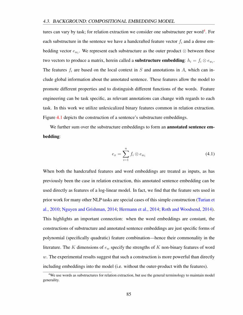
4.3. BACKGROUND: COMPOSITIONAL EMBEDDING MODEL
tures can vary by task; for relation extraction we consider one substructure per word4. For
each substructure in the sentence we have a handcrafted feature vector fi and a dense em-
bedding vector ewi. We represent each substructure as the outer product ⊗ between these
two vectors to produce a matrix, herein called a substructure embedding: hi = fi ⊗ ewi.
The features fi are based on the local context in S and annotations in A, which can in-
clude global information about the annotated sentence. These features allow the model to
promote different properties and to distinguish different functions of the words. Feature
engineering can be task specific, as relevant annotations can change with regards to each
task. In this work we utilize unlexicalized binary features common in relation extraction.
Figure 4.1 depicts the construction of a sentence’s substructure embeddings.
We further sum over the substructure embeddings to form an annotated sentence em-
bedding:
ex =n∑
i=1
fi ⊗ ewi(4.1)
When both the handcrafted features and word embeddings are treated as inputs, as has
previously been the case in relation extraction, this annotated sentence embedding can be
used directly as features of a log-linear model. In fact, we find that the feature sets used in
prior work for many other NLP tasks are special cases of this simple construction (Turian et
al., 2010; Nguyen and Grishman, 2014; Hermann et al., 2014; Roth and Woodsend, 2014).
This highlights an important connection: when the word embeddings are constant, the
constructions of substructure and annotated sentence embeddings are just specific forms of
polynomial (specifically quadratic) feature combination—hence their commonality in the
literature. The K dimensions of ew specify the strengths of K non-binary features of word
w. The experimental results suggest that such a construction is more powerful than directly
including embeddings into the model (i.e. without the outer-product with the features).
4We use words as substructures for relation extraction, but use the general terminology to maintain modelgenerality.
85
4.3. BACKGROUND: COMPOSITIONAL EMBEDDING MODEL
4.3.2 The Log-Bilinear Model
The full log-bilinear model first forms the substructure and annotated sentence embeddings
from the previous subsection. The model uses its parameters to score the annotated sen-
tence embedding and uses a softmax to produce an output label. We call the entire model
the Feature-rich Compositional Embedding Model (FCM).
Our task is to determine the label y (relation) given the instance x = (M1,M2, S, A).
We formulate this as a probability.
pFCM(y|x;T, e) =exp
(∑ni=1 ⟨Ty, fwi
⊗ ewi⟩F)
Z(x)(4.2)
where ⟨·, ·⟩F is the ‘matrix dot product’ or Frobenius inner product of the two matrices.
The normalizing constant which sums over all possible output labels y′ ∈ L is given by
Z(x) =∑
y′∈L exp(∑n
i=1 ⟨Ty′ , fwi⊗ ewi
⟩F). The parameters of the model are the word
embeddings e for each word type and a list of weight matrices T = [Ty]y∈L which is used
to score each label y. The model is log-bilinear (i.e. log-quadratic) since we recover a
log-linear model by fixing either e or T . This chapter studies both the full log-bilinear and
the log-linear model obtained by treating the word embeddings as constant rather than as
parameters of the model.
Other popular log-bilinear models are the log-bilinear language models (Mnih and Hin-
ton, 2007; Mikolov et al., 2013). The Log-Bilinear Language Model (LBLM) of Mnih and
Hinton (2007) provides a model p(wn|w1, w2, . . . , wn−1) where w1, w2, . . . , wn−1 are the
context words and wn is the predicted word. In the LBLM, the bilinear interaction is be-
tween the word embeddings of the context words and the embedding vector of the predicted
word. By contrast, the bilinear interaction in our FCM model is between the word embed-
dings ewiand the parameter tensor Ty as described above.
86

4.3. BACKGROUND: COMPOSITIONAL EMBEDDING MODEL
4.3.3 Discussion of the Compositional Model
Substructure Embeddings Similar words (i.e. those with similar embeddings) with sim-
ilar functions in the sentence (i.e. those with similar features) will have similar matrix rep-
resentations. To understand the selection of the outer product, consider the example in Fig.
4.1. The word “driving” can indicate the ART relation if it appears on the dependency path
between M1 and M2. Suppose the third feature in fwiindicates this on-path feature.
The FCM can now learn parameters that give the third row a high weight for the ART la-
bel. Other words with embeddings similar to “driving” that appear on the dependency path
between the mentions will similarly receive high weight for the ART label. On the other
hand, if the embedding is similar but is not on the dependency path, it will have 0 weight.
Thus, the model generalizes its model parameters across words with similar embeddings
only when they share similar functions in the sentence.
Smoothed Lexical Features Another intuition about the selection of outer product is
that it is actually a smoothed version of traditional lexical features used in classical NLP
systems. Consider a lexical feature f = u∧w, which is a conjunction (logic-and) between
non-lexical property u and lexical part (word)w. If we representw as a one-hot vector, then
the outer product exactly recovers the original feature f . Then if we replace the one-hot
representation with its word embedding, we get the current form of the FCM. Therefore, the
model can be viewed as a smoothed version of lexical features, which keeps the expressive
strength, and uses embeddings to generalize to low frequency features.
Time Complexity Inference in FCM is much faster than both CNNs (Collobert et al.,
2011b) and RNNs (Socher et al., 2013b; Bordes et al., 2012). FCM requires O(nds)
products on average, where n is the length of the sentence, d is the dimension of word
embedding, and s is the average number of per-word non-zero feature values. That is,
s = 1n
∑ni=1
∑j fi,j where fi in our models is a sparse binary feature vector. In contrast,
87

4.4. A LOG-LINEAR MODEL
CNNs and RNNs usually have complexity O(C · nd2), where C is a model dependent
constant.
4.4 A Log-linear Model
Our log-linear model uses a rich binary feature set from Sun et al. (2011) (Baseline)—this
consists of all the baseline features of Zhou et al. (2005) plus several additional carefully-
chosen features that have been highly tuned for ACE-style relation extraction over years of
research. We exclude the Country gazetteer and WordNet features from Zhou et al. (2005).
For a detailed description of the features, we direct the reader to Zhou et al. (2005) and Sun
et al. (2011). Here, we provide a summary of the types of context considered by them:
• The words of each mention, their head words, and combinations of these
• Words in between the mentions plus indicators of the number of words intervening
• Words appearing immediately before or after the mentions
• Entity types and phrase types of the mentions
• Counts of the number of intervening mentions
• Indicators for whether the mentions overlap and their direction
• Features based on the heads of the chunks intervening between the mentions, before
or after the mentions
• Combinations of labels of the chunks between the mentions
• Features combining information from a dependency tree (e.g. head of mention, de-
pendent of mention) with entity type information
• Features combining information from a constituency tree (e.g. is head contained
within an NP) with entity type information
88

4.5. HYBRID MODEL
• Labels along shortest path through constituency tree
• Bigrams of the words in between the mentions
• The full sequence of words in between the mentions
• Labels of a high cut through the constituency tree
• Parts-of-speech, words, or labels of the shortest dependency tree path between the
mentions
The features incorporate information from entity types, mention types, parts-of-speech, a
dependency tree, constituency tree, and chunking of the sentence. These features differ
from those used for SRL in Section 3.2.5. The reason for the difference is that we selected
the features from the prior state-of-the-art methods for each task; as discussed in Sec-
tion 4.2, the two tasks have qualitative differences and the literature has typically treated
the two tasks as distinct.
The log-linear model has the usual form:
ploglin(y|x) ∝ exp(θ · f(x, y)) (4.3)
where θ are the model parameters and f(x, y) is a vector of features.
4.5 Hybrid Model
We present a product-of-experts model (Hinton, 2002), which combines the FCM (Sec-
tion 4.3.2) with an existing log-linear model (Section 4.4). We do so by defining a new
model:
pFCM+loglin(y|x;T, e,θ) =1
ZpFCM(y|x;T, e) ploglin(y|x;θ) (4.4)
89

4.5. HYBRID MODEL
Yi,j
�
��
✕�fwn�
P(y|x)�
fw1� ew1�
hw1� hwn�
ex�
!!!�
ewn�
!!!�
!!!� !!!�
!!!�!!!�
Figure 4.2: Factor graph of the hybrid model. The variable Yi,j ranges over possible rela-tions for the ith and jth entity mentions in the sentence. The top factor (blue) multiplies inthe score according to a log-linear model. The bottom factor (red) multiplies in the scoreof the FCM, a compositional embedding model—depicted here as a neural network.
The integration treats each model as providing a score which we multiply together. The
constant Z ensures a normalized distribution. In this hybrid model, we assume that the
features for pFCM and ploglin are different, with the latter generally using a much richer feature
set. If the two submodels use the same features, then the hybrid model reduces to an FCM
with ew having an additional dimension that always takes value 1. We can view this as a
very simple factor graph (Section 2.3.1) consisting of just one variable and two factors—
corresponding to the two submodels. This representation of our hybrid model is shown in
Figure 4.2. In this chapter, we do not make use of this factor graph representation, except
as a pedagogical tool for understanding the model. However, in a subsequent chapter,
(Chapter 6), we will consider more complicated hybrid models for which approximate
inference will be run over the factor graph.
To train we optimize a conditional log-likelihood objective (Section 2.3.4.1):
ℓ(D;T, e,θ) =∑
(x,y)∈Dlog p(y|x;T, e,θ)
where D is the set of all training data, e is the set of word embeddings, T is the FCM
tensor parameters, and θ are the parameters of the log-linear model. To optimize the
objective, for each instance (y,x) we perform stochastic training on the loss function
90
4.6. MAIN EXPERIMENTS
ℓ = ℓ(y,x;T, e,θ) = log p(y|x;T, e,θ).
The gradients of the model parameters are obtained by backpropagation (Section 2.2.2)
(i.e. repeated application of the chain rule). For the hybrid model, this is easily computed
since each sub-model has separate parameters. When we treat the word embeddings as
parameters (i.e. the log-bilinear FCM), we also fine-tune the word embeddings with the
FCM model. As is common in deep learning, we initialize these embeddings from a neural
language model and then fine-tune them for our supervised task.
4.6 Main Experiments
Our primary experiments consider two settings: relation extraction on ACE 2005 and rela-
tion classification on SemEval-2010 Task 8.
4.6.1 Experimental Settings
Features Our FCM features (Table 4.2) use a feature vector fwiover the word wi, the two
target entities M1,M2, and their dependency path. Here h1, h2 are the indices of the two
head words of M1,M2, × refers to the Cartesian product between two sets, th1 and th2 are
entity types (named entity tags for ACE 2005 or WordNet supertags for SemEval 2010—
see Table 4.3 for example tags) of the head words of two entities, and ϕ stands for the
empty feature. ⊕ refers to the conjunction of two elements. The In-between features
indicate whether a word wi is in between two target entities, and the On-path features
indicate whether the word is on the dependency path, on which there is a set of words P ,
between the two entities.
We also use the target entity type as a feature. Combining this with the basic features
results in more powerful compound features, which can help us better distinguish the func-
tions of word embeddings for predicting certain relations. For example, if we have a person
and a vehicle, we know it will be more likely that they have an ART relation. For the ART
91

4.6. MAIN EXPERIMENTS
Set TemplateHeadEmb {I[i = h1], I[i = h2]}
(wi is head of M1/M2) ×{ϕ, th1 , th2 , th1 ⊕ th2}Context I[i = h1 ± 1] (left/right token of wh1)
I[i = h2 ± 1] (left/right token of wh2)In-between I[i > h1]&I[i < h2] (in between )
×{ϕ, th1 , th2 , th1 ⊕ th2}On-path I[wi ∈ P ] (on path)
×{ϕ, th1 , th2 , th1 ⊕ th2}
Table 4.2: Feature sets used in FCM.
relation, we introduce a corresponding weight vector, which is closer to lexical embeddings
similar to the embedding of “drive”.
All linguistic annotations needed for features (POS, chunks5, parses) are from Stan-
ford CoreNLP (Manning et al., 2014). Since SemEval does not have gold entity types we
obtained WordNet and named entity tags using Ciaramita and Altun (2006). For all exper-
iments we use 200-d word embeddings trained on the NYT portion of the Gigaword 5.0
corpus (Parker et al., 2011). The embeddings are trained with word2vec6 using the CBOW
model with negative sampling (15 negative words) (Mikolov et al., 2013). We set a window
size c=5, and remove types occurring less than 5 times.
Models We consider several methods. The first three methods (A, B, C) are examples of
either the FCM alone or a standard log-linear model. The two remaining methods (D, E) are
hybrid models that integrate FCM as a submodel within the hybrid model (Section 4.5)—we
consider two such combinations.
(A) FCM (Section 4.3) in isolation without fine-tuning. We use the complete feature
set given in Table 4.2.
(B) FCM (Section 4.3.2) in isolation with fine-tuning (i.e. trained as a log-bilinear
model), using the same feature set as in (A).
5Obtained from the constituency parse using the CONLL 2000 chunking converter (Perl script).6https://code.google.com/p/word2vec/
92

4.6. MAIN EXPERIMENTS
(C) The log-linear model alone (Section 4.4).
(D) A hybrid model combines a restricted form of the FCM with the log-linear model
from (C) above. For the FCM, we restrict to the feature set of Nguyen and Gr-
ishman (2014) obtained by using the embeddings of heads of two entity mentions
(+HeadOnly).
(E) Our full hybrid model which combines the FCM from (A) with the log-linear
model from (C) above.
All models use L2 regularization tuned on dev data.
Datasets and Evaluation
ACE 2005 We evaluate our relation extraction system on the English portion of the ACE
2005 corpus (Walker et al., 2006).7 There are 6 domains: Newswire (nw), Broadcast Con-
versation (bc), Broadcast News (bn), Telephone Speech (cts), Usenet Newsgroups (un),
and Weblogs (wl). Following prior work we focus on the domain adaptation setting, where
we train on one set (the union of the news domains (bn+nw), tune hyperparameters8 on
a dev domain (half of bc) and evaluate on the remainder (cts, wl, and the remainder of
bc) (Plank and Moschitti, 2013; Nguyen and Grishman, 2014). The LDC release of the
ACE data contains four distinct annotations: fp1, fp2, adj, timex2norm. Following Plank
and Moschitti (2013), we use the adjudicated fileset (adj) – these are files which were an-
notated twice and for which discrepancies were resolved.
We assume that gold entity spans and types are available for train and test. We use all
7Many relation extraction systems evaluate on the ACE 2004 corpus (Mitchell et al., 2005). Unfortunately,the most common convention is to use 5-fold cross validation, treating the entirety of the dataset as bothtrain and evaluation data. Rather than continuing to overfit this data by perpetuating the cross-validationconvention, we instead focus on ACE 2005.
8For each ACE 2005 model, we performed a grid-search over hyperparameters and selected the modelwhich obtained the highest F1 on the development set. There were four hyperparameters tuned by the gridsearch: (1) the variance of the L2 regularizer σ2 ∈ {40000, 400000}, (2) a constant γ ∈ {0.1, 1, 10} usedto scale the initial embeddings after they were renormalized to sum-to-one, (3) the AdaGrad learning rateη ∈ {0.01, 0.1}, and (4) AdaGrad’s initial value for the sum of the squares δ ∈ {0.1, 1}.
93

4.6. MAIN EXPERIMENTS
pairs of entity mentions to yield 43,497 total relations in the training set, of which 3,658
are non-nil. One curious aspect of the ACE data is that some relations are self-referential.
That is, the pair of entities is some entity and itself. We also included these self-referential
relations so that the number of non-nil relations would be identical to that reported in the
original ACE dataset. We did not include any negative examples of self-referential rela-
tions. We followed Table 6 of the ACE 2005 annotation guidelines to determine which of
the relations should be treated as symmetric (METONYMY, PER-SOC, and PHYS) and
asymmetric (ART, GEN-AFF, ORG-AFF, and PART-WHOLE). The nil relation is treated
as symmetric. Thus, the total output space for our models would be 12 labels, but the
METONYMY relation never appears in any explicit relation mentions in the ACE dataset.
So the total number of observed labels in the training data is only 11. We report precision,
recall, and micro F1 for relation extraction. While it is not our focus, for completeness
we include results with unknown entity types following Plank and Moschitti (2013) (Sec-
tion 4.7).
SemEval 2010 Task 8 We evaluate on the SemEval 2010 Task 8 dataset9 (Hendrickx et
al., 2010) to compare with other compositional models and highlight the advantages of our
models. This task is to determine the relation type (or no relation) between two entities in
a sentence. We adopt the setting of Socher et al. (2012). We use 10-fold cross validation
on the training data to select hyperparameters and do regularization by early stopping. The
learning rates for FCM with/without fine-tuning are 5e-3 and 5e-2 respectively. We report
macro-F1 and compare to previously published results.
As noted earlier, we distinguish between two tasks: ACE 2005 relation extraction and
SemEval 2010 Task 8 relation classification. The key distinction between them is the pro-
portion of entity pairs that are labeled as having no relation. In the ACE 2005 training set,
only 10.1% of training instances are non-nil relations, the rest are nil. In the SemEval data,
82.6% of the instances are labeled with one of the 9 standard relations and 17.4% relations9http://docs.google.com/View?docid=dfvxd49s_36c28v9pmw
94

4.6. MAIN EXPERIMENTS
Tag Type # Tags Example Tags
AC
E20
05
Types 7 FAC, GPE, LOC, ORG, PER, VEH, WEA
Subtypes 43 FAC:Airport, FAC:Building-Grounds,FAC:Path, FAC:Plant, FAC:Subarea-Facility, GPE:Continent, GPE:County-or-District, GPE:GPE-Cluster, GPE:Nation,GPE:Population-Center, . . .
Sem
Eva
l201
0Ta
sk8
NER 50 E ANIMAL, E DISEASE,E EVENT OTHER, E FAC DESC AIRPORT,E FAC DESC BRIDGE,E FAC DESC BUILDING,E FAC DESC HIGHWAY STREET,E FAC DESC OTHER, E GAME,E GPE CITY, . . .
WordNet 46 adj.all, adj.pert, adj.ppl, adv.all, noun.Tops,noun.act, noun.animal, noun.artifact,noun.attribute, noun.body, . . .
Table 4.3: Named entity tags for ACE 2005 and SemEval 2010 Task 8. The ACE 2005subtypes are only shown for reference: all of our features referred to the types only.
are labeled as Other (a category which could include nil relations).
4.6.2 Results
ACE 2005 Despite FCM’s (A) simple feature set (see Table 4.2), it is competitive with
the log-linear baseline (C) on out-of-domain test sets (Table 4.4). In the typical gold entity
spans and types setting, both Plank and Moschitti (2013) and Nguyen and Grishman (2014)
found that they were unable to obtain improvements by adding embeddings to baseline
feature sets. By contrast, we find that on all domains the combination baseline + FCM (E)
obtains the highest F1 and significantly outperforms the other baselines, yielding the best
reported results for this task. We found that fine-tuning of embeddings (B) did not yield
improvements on our out-of-domain development set, in contrast to our results below for
SemEval. We suspect this is because fine-tuning allows the model to overfit the training
domain, which then hurts performance on the unseen ACE test domains. Accordingly,
95

4.6. MAIN EXPERIMENTS
bcct
sw
lAv
g.M
odel
PR
F1P
RF1
PR
F1F1
(A)
FC
M-o
nly
(ST
)66
.56
57.8
661
.90
65.6
244
.35
52.9
357
.80
44.6
250
.36
55.0
6(C
)B
asel
ine
(ST
)74
.89
48.5
458
.90
74.3
240
.26
52.2
363
.41
43.2
051
.39
54.1
7(D
)+
Hea
dOnl
y(S
T)
70.8
750
.76
59.1
671
.16
43.2
153
.77
57.7
142
.92
49.2
354
.05
(E)
+F
CM
(ST
)74
.39
55.3
563
.48
74.5
345
.01
56.1
265
.63
47.5
955
.17
58.2
6
Tabl
e4.
4:C
ompa
riso
nof
mod
els
onA
CE
2005
out-
of-d
omai
nte
stse
ts.
Bas
elin
e+
Hea
dOnl
yis
our
reim
plem
enta
tion
ofth
efe
atur
esof
Ngu
yen
and
Gri
shm
an(2
014)
.
96

4.6. MAIN EXPERIMENTS
Table 4.4 shows only the log-linear model.
Finally, we highlight an important contrast between FCM (A) and the log-linear model
(C): the latter uses over 50 feature templates based on a POS tagger, dependency parser,
chunker, and constituency parser. The resulting model has about 6.5 million parameters.
FCM uses only a dependency parse and about 0.5 million parameters (not including the
embeddings, which are held constant) but still obtains better results (Avg. F1).
SemEval 2010 Task 8 Table 4.5 compares our models to the best reported results from
the SemEval-2010 Task 8 shared task and several other compositional models.
For the FCM we considered two feature sets. We found that using NE tags instead
of WordNet tags helps with fine-tuning but hurts without. This may be because the set
of WordNet tags is larger making the model more expressive, but also introduces more
parameters. When the embeddings are fixed, they can help to better distinguish different
functions of embeddings. But when fine-tuning, it becomes easier to over-fit. Alleviating
over-fitting is a subject for future work (Section 4.9).
With either WordNet or NER features, FCM achieves better performance than the RNN
and MVRNN. With NER features and fine-tuning, it outperforms a CNN (Zeng et al.,
2014) and also the combination of an embedding model and a traditional log-linear model
(RNN/MVRNN + linear) (Socher et al., 2012). As with ACE, FCM uses less linguistic
resources than many close competitors (Rink and Harabagiu, 2010).
We also compared to concurrent work on enhancing the compositional models with
task-specific information for relation classification, including Hashimoto et al. (2015) (RelEmb),
which trained task-specific word embeddings, and Santos et al. (2015) (CR-CNN), which
proposed a task-specific ranking-based loss function. Our Hybrid methods (FCM + linear)
get comparable results to theirs. Note that their base compositional model results without
any task-specific enhancements, i.e. RelEmb with word2vec embeddings and CR-CNN
with log-loss, are still lower than the best FCM result. Our main finding is that the hybrid
97

4.6. MAIN EXPERIMENTS
Cla
ssifi
erFe
atur
esF1
SVM
(Rin
kan
dH
arab
agiu
,201
0)PO
S,pr
efixe
s,m
orph
olog
ical
,Wor
dNet
,dep
ende
ncy
pars
e,82
.2(B
esti
nSe
mE
val2
010)
Lev
incl
asse
d,Pr
oBan
k,Fr
ameN
et,N
omL
ex-P
lus,
Goo
gle
n-gr
am,p
arap
hras
es,T
extR
unne
rR
NN
wor
dem
bedd
ing,
synt
actic
pars
e74
.8R
NN
+lin
ear
wor
dem
bedd
ing,
synt
actic
pars
e,PO
S,N
ER
,Wor
dNet
77.6
MV
RN
Nw
ord
embe
ddin
g,sy
ntac
ticpa
rse
79.1
MV
RN
N+
linea
rw
ord
embe
ddin
g,sy
ntac
ticpa
rse,
POS,
NE
R,W
ordN
et82
.4C
NN
(Zen
get
al.,
2014
)w
ord
embe
ddin
g,W
ordN
et82
.7C
R-C
NN
(log
-los
s)w
ord
embe
ddin
g82
.7C
R-C
NN
(ran
king
-los
s)w
ord
embe
ddin
g84
.1R
elE
mb
(wor
d2ve
cem
bedd
ing)
wor
dem
bedd
ing
81.8
Rel
Em
b(t
ask-
spec
embe
ddin
g)w
ord
embe
ddin
g82
.8R
elE
mb
(tas
k-sp
ecem
bedd
ing)
+lin
ear
wor
dem
bedd
ing,
depe
nden
cypa
ths,
Wor
dNet
,NE
83.5
Dep
NN
wor
dem
bedd
ing,
depe
nden
cypa
ths
82.8
Dep
NN
+lin
ear
wor
dem
bedd
ing,
depe
nden
cypa
ths,
Wor
dNet
,NE
R83
.6
(A)
FC
M(l
og-l
inea
r)w
ord
embe
ddin
g,de
pend
ency
pars
e,W
ordN
et82
.0w
ord
embe
ddin
g,de
pend
ency
pars
e,N
ER
81.4
(B)
FC
M(l
og-b
iline
ar)
wor
dem
bedd
ing,
depe
nden
cypa
rse,
Wor
dNet
82.5
wor
dem
bedd
ing,
depe
nden
cypa
rse,
NE
R83
.0
(E)
FC
M(l
og-l
inea
r)+
linea
r(H
ybri
d)w
ord
embe
ddin
g,de
pend
ency
pars
e,W
ordN
et83
.1w
ord
embe
ddin
g,de
pend
ency
pars
e,N
ER
83.4
Tabl
e4.
5:C
ompa
riso
nof
ourm
odel
sw
ithpr
evio
usly
publ
ishe
dre
sults
forS
emE
val2
010
Task
8.
98

4.7. ADDITIONAL ACE 2005 EXPERIMENTS
model again performs better than either of its submodels alone.
Finally, a concurrent work (Liu et al., 2015) proposes DepNN, which builds representa-
tions for the dependency path (and its attached subtrees) between two entities by applying
recursive and convolutional neural networks successively. Compared to their model, the
FCM achieves comparable results. Of note, the FCM and the RelEmb are also the most effi-
cient models among all above compositional models since they have linear time complexity
with respect to the dimension of embeddings.
4.7 Additional ACE 2005 Experiments
Next we present results in a distinct setting for ACE 2005 in which the gold entity types are
not available. This allows for additional comparison with prior work (Plank and Moschitti,
2013).
4.7.1 Experimental Settings
Data For comparison with Plank and Moschitti (2013), we (1) generate relation instances
from all pairs of entities within each sentence with three or fewer intervening entity mentions—
labeling those pairs with no relation as negative instances, (2) use gold entity spans (but not
types) at train and test time, and (3) evaluate on the 7 coarse relation types, ignoring the
subtypes. In the training set, 34,669 total relations are annotated of which only 3,658 are
non-nil relations. We did not match the number of tokens they reported in the cts and wl
domains. Therefore, in this section we only report the results on the test set of bc domain.
Models and Features We run the same models as in Section 4.6.2 on this task. Here
the FCM does not use entity type features. Plank and Moschitti (2013) also use Brown
clusters and word vectors learned by latent-semantic analysis (LSA). In order to make a fair
comparison with their method, we also report the FCM result using Brown clusters (prefixes
99

4.7. ADDITIONAL ACE 2005 EXPERIMENTS
of length 5) of entity heads as entity types. Furthermore, we report non-comparable settings
using WordNet super-sense tags of entity heads as types. The WordNet features were also
used in their paper but not as substitution of entity types. We use the same toolkit to get the
WordNet tags as in Section 4.6.1. The Brown clusters are from (Koo et al., 2008)10.
4.7.2 Results
Table 4.6 shows the results under the low-resource setting. When no entity types are avail-
able, the performance of the FCM-only model greatly decreases to 48.15%, which is con-
sistent with our observation in the ablation tests. The baseline model also relies heavily
on the entity types: without entity type information the performance of our baseline model
drop to 40.62%, even lower than the reduced FCM only model.
The combination of baseline model and head embeddings (Baseline + HeadOnly) greatly
improve the results. This is consistent with the observation in Nguyen and Grishman (2014)
that when the gold entity types are unknown, information of the entity heads provided by
their embeddings will play a more important role. Combination of the baseline and FCM
(Baseline + FCM) also achieves improvement but not significantly better than Baseline +
HeadOnly. A possible explanation is that FCM becomes less efficient on using context
word embeddings when the entity type information is unavailable. In this situation the
head embeddings provided by FCM become the dominating contribution to the baseline
model, making the model have similar behavior as the Baseline + HeadOnly method.
Finally, we find Brown clusters can help FCM when entity types are unknown. Although
the performance is still not significantly better than Baseline + HeadOnly, it outperforms
all the results in Plank and Moschitti (2013) as a single model, and with the same source
of features. WordNet super-sense tags further improve FCM, and achieves the best reported
results on this low-resource setting. These results are encouraging since it shows FCM may
be more useful under the end-to-end setting where predictions of both entity mentions and
10http://people.csail.mit.edu/maestro/papers/bllip-clusters.gz
100

4.8. RELATED WORK
bcModel P R F1PM’13 (Brown) 54.4 43.4 48.3PM’13 (LSA) 53.9 45.2 49.2PM’13 (Combination) 55.3 43.1 48.5(A) FCM only 53.7 43.7 48.2(C) Baseline 59.4 30.9 40.6(E) + HeadOnly 64.9 41.3 50.5(E) + FCM 65.5 41.5 50.8(A) FCM only w/ Brown 64.6 40.2 49.6(A) FCM only w/WordNet 64.0 43.2 51.6Linear+Emb 46.5 49.3 47.8Tree-kernel+Emb (Single) 57.6 46.6 51.5Tree-kernel+Emb (Combination) 58.5 47.3 52.3
Table 4.6: Comparison of models on ACE 2005 out-of-domain test sets for the low-resourcesetting, where the gold entity spans are known but entity types are unknown. PM’13 is theresults reported in Plank and Moschitti (2013). “Linear+Emb” is the implementation of ourmethod (4) in (Nguyen et al., 2015). The “Tree-kernel+Emb” methods are the enrichmentsof tree-kernels with embeddings proposed by Nguyen et al. (2015).
relation mentions are required in place of predicting relation based on gold tags (Li and Ji,
2014).
Recently Nguyen et al. (2015) proposed a novel way of applying embeddings to tree-
kernels. From the results, our best single model achieves comparable result with their best
single system, while their combination method is slightly better than ours. This suggests
that we may benefit more from combining the usages of multiple word representations; and
we will investigate it in future work.
4.8 Related Work
Compositional Models for Sentences In order to build a representation (embedding)
for a sentence based on its component word embeddings and structural information, recent
work on compositional models (stemming from the deep learning community) has designed
model structures that mimic the structure of the input. For example, these models could
101

4.8. RELATED WORK
take into account the order of the words (as in Convolutional Neural Networks (CNNs))
(Collobert et al., 2011b) or build off of an input tree (as in Recursive Neural Networks
(RNNs) or the Semantic Matching Energy Function) (Socher et al., 2013b; Bordes et al.,
2012).
While these models work well on sentence-level representations, the nature of their
designs also limits them to fixed types of substructures from the annotated sentence, such as
chains for CNNs and trees for RNNs. Such models cannot capture arbitrary combinations
of linguistic annotations available for a given task, such as word order, dependency tree,
and named entities used for relation extraction. Moreover, these approaches ignore the
differences in functions between words appearing in different roles. This does not suit more
general substructure labeling tasks in NLP, e.g. these models cannot be directly applied
to relation extraction since they will output the same result for any pair of entities in a
same sentence. By contrast, the FCM annotates the sentence with the entity pair before
embedding it, so that the embedding is of the entire annotated sentence.
Compositional Models with Annotation Features To tackle the problem of traditional
compositional models, Socher et al. (2012) made the RNN model specific to relation extrac-
tion tasks by working on the minimal subtree that spans the two target entities. However,
these specializations to relation extraction do not generalize easily to other tasks in NLP.
There are two ways to achieve such specialization in a more general fashion:
1. Enhancing Compositional Models with Features. A recent trend enhances composi-
tional models with annotation features. Such an approach has been shown to significantly
improve over pure compositional models. For example, Hermann et al. (2014) and Nguyen
and Grishman (2014) gave different weights to words with different syntactic context types
or to entity head words with different argument IDs. Zeng et al. (2014) use concatenations
of embeddings as features in a CNN model, according to their positions relative to the target
entity mentions. Belinkov et al. (2014) enrich embeddings with linguistic features before
102
4.9. SUMMARY
feeding them forward to a RNN model. Socher et al. (2013a) and Hermann and Blunsom
(2013) enhanced RNN models by refining the transformation matrices with phrase types
and CCG super tags.
2. Engineering of Embedding Features. A different approach to combining traditional
linguistic features and embeddings is hand-engineering features with word embeddings and
adding them to log-linear models. Such approaches have achieved state-of-the-art results
in many tasks including NER, chunking, dependency parsing, semantic role labeling, and
relation extraction (Miller et al., 2004; Turian et al., 2010; Koo et al., 2008; Roth and
Woodsend, 2014; Sun et al., 2011; Plank and Moschitti, 2013). Roth and Woodsend (2014)
considered features similar to ours for semantic role labeling.
However, in prior work both of above approaches are only able to utilize limited infor-
mation, usually one property for each word. Yet there may be different useful properties
of a word that can contribute to the performances of the task. By contrast, our model can
easily utilize these features without changing the model structures.
Task-Specific Enhancements for Relation Classification An orthogonal direction of
improving compositional models for relation classification is to enhance the models with
task-specific information. For example, Hashimoto et al. (2015) trained task-specific word
embeddings, and Santos et al. (2015) proposed a ranking-based loss function for relation
classification.
4.9 Summary
We have presented a new hybrid model for combining a log-linear model with the FCM, a
compositional model for deriving sentence-level and substructure embeddings from word
embeddings. Compared to existing compositional models, our hybrid model can easily
handle arbitrary types of input and handle global information for composition, while re-
maining easy to implement. We have demonstrated that the compositional model FCM
103

4.9. SUMMARY
alone attains near state-of-the-art performances on several relation extraction tasks, and in
combination with traditional feature based log-linear models it obtains state-of-the-art re-
sults. On an cross-domain setting for ACE 2005, the FCM obtains 55.06 Avg. F1 and the
hybrid gets 58.26 Avg. F1. On SemEval 2010 Task 8, the FCM gets 83.0 F1 and the hybrid
model obtains 83.4 F1.
104

Chapter 5
Approximation-aware Learning for
Structured Belief Propagation
Having motivated the use of latent variables, structured factors, and neural factors, we turn
to the remaining problem: learning with inexact inference. Of course, it is possible to
build effective models without resorting to inexact inference—the previous two chapters
exemplified this fact. However, joint modeling is fundamentally about enabling factors that
express opinions about wider contexts of variables. Doing so is what leads to the sort of
high treewidth models that require approximate inference.
This chapter1 develops a learning framework that will cope with inexact marginal in-
ference in the types of structured models that we care about. Viewed under a different lens,
this chapter is about defining new models that resemble neural networks whose topology is
inspired by structured belief propagation run on a graphical model. Though joint modeling
is our end goal, we currently consider a simpler class of models for which approximate
inference is fast, but for which we also have efficient exact inference algorithms. This
allows us to better study the behavior of our new learning algorithm for structured belief
propagation.
1A previous version of this work was presented in Gormley et al. (2015a).
105

5.1. INTRODUCTION
We show how to train the fast dependency parser of Smith and Eisner (2008) for im-
proved accuracy. This parser can consider higher-order interactions among edges while re-
taining O(n3) runtime. It outputs the parse with maximum expected recall—but for speed,
this expectation is taken under a posterior distribution that is constructed only approxi-
mately, using loopy belief propagation through structured factors. We show how to adjust
the model parameters to compensate for the errors introduced by this approximation, by
following the gradient of the actual loss on training data. We find this gradient by back-
propagation. That is, we treat the entire parser (approximations and all) as a differentiable
circuit, as others have done for loopy CRFs (Domke, 2010; Stoyanov et al., 2011; Domke,
2011; Stoyanov and Eisner, 2012). The resulting parser obtains higher accuracy with fewer
iterations of belief propagation than one trained by conditional log-likelihood.
5.1 Introduction
Recent improvements to dependency parsing accuracy have been driven by higher-order
features. Such a feature can look beyond just the parent and child words connected by a
single edge to also consider siblings, grandparents, etc. By including increasingly global
information, these features provide more information for the parser—but they also com-
plicate inference. The resulting higher-order parsers depend on approximate inference and
decoding procedures, which may prevent them from predicting the best parse.
For example, consider the dependency parser we will train in this chapter, which is
based on the work of Smith and Eisner (2008). Ostensibly, this parser finds the minimum
Bayes risk (MBR) parse under a probability distribution defined by a higher-order depen-
dency parsing model. In reality, it achieves O(n3tmax) runtime by relying on three approx-
imations during inference: (1) variational inference by loopy belief propagation (BP) on
a factor graph, (2) truncating inference after tmax iterations prior to convergence, and (3)
a first-order pruning model to limit the number of edges considered in the higher-order
106
5.1. INTRODUCTION
model. Such parsers are traditionally trained as if the inference had been exact.2
In contrast, we train the parser such that the approximate system performs well on the
final evaluation function. We treat the entire parsing computation as a differentiable circuit,
and backpropagate the evaluation function through our approximate inference and decoding
methods to improve its parameters by gradient descent. The system also learns to cope
with model misspecification, where the model couldn’t perfectly fit the distribution even
absent the approximations. For standard graphical models, Stoyanov and Eisner (2012)
call this approach ERMA, for “empirical risk minimization under approximations.” For
objectives besides empirical risk, Domke (2011) refers to it as “learning with truncated
message passing.”3
Our primary contribution is the application of this approximation-aware learning method
in the parsing setting, for which the graphical model involves a global constraint. Smith
and Eisner (2008) previously showed how to run BP in this setting (by calling the inside-
outside algorithm as a subroutine). We must backpropagate the downstream objective func-
tion through their algorithm so that we can follow its gradient. We carefully define an em-
pirical risk objective function (a la ERMA) to be smooth and differentiable, yet equivalent
to accuracy of the minimum Bayes risk (MBR) parse in the limit. Finding this difficult to
optimize, we introduce a new simpler objective function based on the L2 distance between
the approximate marginals and the “true” marginals from the gold data.
The goal of this work is to account for the approximations made by a system rooted
in structured belief propagation. Taking such approximations into account during training
enables us to improve the speed and accuracy of inference at test time. We compare our
training method with the standard approach of conditional log-likelihood (CLL) training.
2For perceptron training, utilizing inexact inference as a drop-in replacement for exact inference can badlymislead the learner (Kulesza and Pereira, 2008; Huang et al., 2012).
3A related approach that we do not explore here are the BP Inference Machines (BPIM) of Ross et al.(2011). Unlike ERMA (Stoyanov et al., 2011) and truncated message passing (Domke, 2011), BPIMs dis-pense with the standard message passing equations and instead train a sequence of logistic regressors to outputaccurate messages directly. Like our work, BPIMs define a differentiable computation and the approximatesystem can be trained end-to-end with backpropagation.
107

5.2. DEPENDENCY PARSING BY BELIEF PROPAGATION
0 2 1 3 4 Juan su abdica reino $
Y2,1 Y1,2 Y3,2 Y2,3
Y3,1 Y1,3
Y4,3 Y3,4
Y4,2 Y2,4
Y4,1 Y1,4
Y0,1
Y0,3
Y0,4
Y0,2
Figure 5.1: Factor graph for dependency parsing of a 4-word sentence; $ is the root ofthe dependency graph. The boolean variable Yh,m encodes whether the edge from parenth to child m is present. The unary factor (black) connected to this variable scores theedge in isolation (given the sentence). The PTREE factor (red) coordinates all variables toensure that the edges form a tree. The drawing shows a few higher-order factors (purple forgrandparents, green for arbitrary siblings); these are responsible for the graph being cyclic(“loopy”).
We evaluate our parser on 19 languages from the CoNLL-2006 (Buchholz and Marsi, 2006)
and CoNLL-2007 (Nivre et al., 2007) Shared Tasks as well as the English Penn Treebank
(Marcus et al., 1993). On English, the resulting parser obtains higher accuracy with fewer
iterations of BP than CLL. On the CoNLL languages, we find that on average it yields
higher accuracy parsers than CLL, particularly when limited to few BP iterations.
5.2 Dependency Parsing by Belief Propagation
This section describes the parser that we will train.
Model A factor graph (Frey et al., 1997; Kschischang et al., 2001) (as described in Sec-
tion 2.3.1) defines the factorization of a probability distribution over a set of variables
108

5.2. DEPENDENCY PARSING BY BELIEF PROPAGATION
{Y1, Y2, . . .}. It is a bipartite graph between variables Yi and factors α. Edges connect
each factor α to a subset of the variables {Yα1 , Yα2 , . . .}, called its neighbors. Each fac-
tor defines a potential function ψα, which assigns a nonnegative score to each configura-
tion of its neighbors yα = {yα1 , yα2 , . . .}. We define the probability of a given assign-
ment y = {y1, y2, . . .} to be proportional to the product of all factors’ potential functions:
p(y) = 1Z
∏α ψα(yα).
Smith and Eisner (2008) define a factor graph for dependency parsing of a given n-word
sentence: n2 binary variables indicate which of the directed arcs are included (yi = ON)
or excluded (yi = OFF) in the dependency parse. One of the factors plays the role of a hard
global constraint: ψPTREE(y) is 1 or 0 according to whether the assignment encodes a pro-
jective dependency tree. Another n2 factors (one per variable) evaluate the individual arcs
given the sentence, so that p(y) describes a first-order dependency parser. A higher-order
parsing model is achieved by also including higher-order factors, each scoring configu-
rations of two or more arcs, such as grandparent and sibling configurations. Higher-order
factors tend to create cycles in the factor graph. See Figure 5.1 for an example factor graph.
We define each potential function to have a log-linear form: ψα(yα) = exp(θ·fα(yα,x)).
Here x is the assignment to the observed variables such as the sentence and its POS tags;
fα extracts a vector of features; and θ is our vector of model parameters. We write the
resulting probability distribution over parses as pθ(y | x), to indicate that it depends on θ.
Loss For dependency parsing, our loss function is the number of missing edges in the
predicted parse y, relative to the reference (or “gold”) parse y∗:
ℓ(y,y∗) =∑
i: yi=OFF I(y∗i = ON) (5.1)
I is the indicator function. Because y and y∗ each specify exactly one parent per word
token, ℓ(y,y∗) equals the directed dependency error: the number of word tokens whose
parent is predicted incorrectly.
109

5.2. DEPENDENCY PARSING BY BELIEF PROPAGATION
Decoder To obtain a single parse as output, we use a minimum Bayes risk (MBR) de-
coder (Section 2.3.2 contained a more general discussion of MBR decoding), which returns
the tree with minimum expected loss under the model’s distribution (Bickel and Doksum,
1977; Goodman, 1996). Our ℓ gives the decision rule:
hθ(x) = argminy
Ey∼pθ(·|x)[ℓ(y,y)] (5.2)
= argmaxy
∑
i: yi=ON
pθ(yi = ON | x) (5.3)
Here y ranges over well-formed parses. Thus, our parser seeks a well-formed parse hθ(x)
whose individual edges have a high probability of being correct according to pθ (since it
lacks knowledge y∗ of which edges are truly correct). MBR is the principled way to take a
loss function into account under a probabilistic model. By contrast, maximum a posteriori
(MAP) decoding does not consider the loss function. It would return the single highest-
probability parse even if that parse, and its individual edges, were unlikely to be correct.4
All systems in this chapter use MBR decoding to consider the loss function at test
time. This implies that the ideal training procedure would be to find the true pθ so that its
marginals can be used in (5.3). Our baseline system attempts this. Yet in practice, we will
not be able to find the true pθ (model misspecification) nor exactly compute the marginals
of pθ (computational intractability). Thus, this chapter proposes a training procedure that
compensates for the system’s approximations, adjusting θ to reduce the actual loss of hθ(x)
as measured at training time.
To find the MBR parse, we first run inference to compute the marginal probability
pθ(yi = ON | x) for each edge. Then we maximize (5.3) by running a first-order depen-
dency parser with edge scores equal to those probabilities.5 When our inference algorithm
is approximate, we replace the exact marginal with its approximation—the belief from BP,
4If we used a simple 0-1 loss function within (5.2), then MBR decoding would reduce to MAP decoding.5Prior work (Smith and Eisner, 2008; Bansal et al., 2014) used the log-odds ratio log pθ(yi=ON)
pθ(yi=OFF) as theedge scores for decoding, but this yields a parse different from the MBR parse.
110
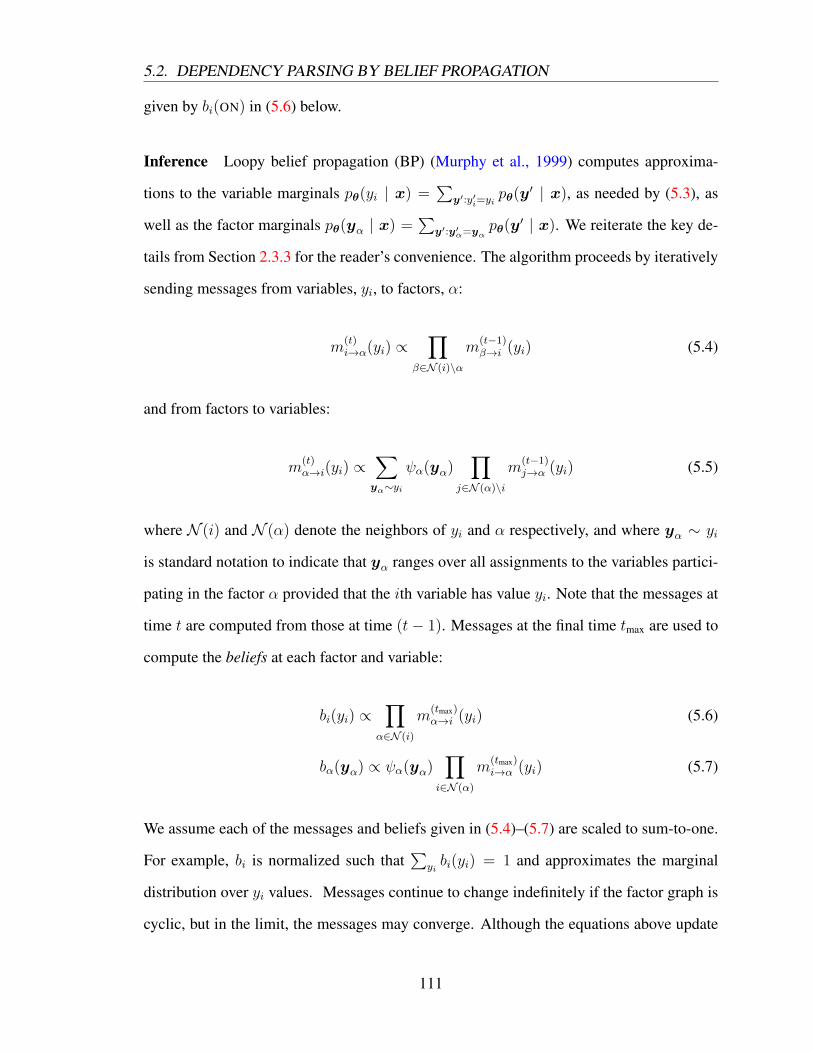
5.2. DEPENDENCY PARSING BY BELIEF PROPAGATION
given by bi(ON) in (5.6) below.
Inference Loopy belief propagation (BP) (Murphy et al., 1999) computes approxima-
tions to the variable marginals pθ(yi | x) =∑
y′:y′i=yipθ(y
′ | x), as needed by (5.3), as
well as the factor marginals pθ(yα | x) = ∑y′:y′α=yα
pθ(y′ | x). We reiterate the key de-
tails from Section 2.3.3 for the reader’s convenience. The algorithm proceeds by iteratively
sending messages from variables, yi, to factors, α:
m(t)i→α(yi) ∝
∏
β∈N (i)\αm
(t−1)β→i (yi) (5.4)
and from factors to variables:
m(t)α→i(yi) ∝
∑
yα∼yiψα(yα)
∏
j∈N (α)\im
(t−1)j→α (yi) (5.5)
where N (i) and N (α) denote the neighbors of yi and α respectively, and where yα ∼ yi
is standard notation to indicate that yα ranges over all assignments to the variables partici-
pating in the factor α provided that the ith variable has value yi. Note that the messages at
time t are computed from those at time (t− 1). Messages at the final time tmax are used to
compute the beliefs at each factor and variable:
bi(yi) ∝∏
α∈N (i)
m(tmax)α→i (yi) (5.6)
bα(yα) ∝ ψα(yα)∏
i∈N (α)
m(tmax)i→α (yi) (5.7)
We assume each of the messages and beliefs given in (5.4)–(5.7) are scaled to sum-to-one.
For example, bi is normalized such that∑
yibi(yi) = 1 and approximates the marginal
distribution over yi values. Messages continue to change indefinitely if the factor graph is
cyclic, but in the limit, the messages may converge. Although the equations above update
111

5.3. APPROXIMATION-AWARE LEARNING
all messages in parallel, convergence is much faster if only one message is updated per
timestep, in some well-chosen serial order.6
For the PTREE factor, the summation over variable assignments required for m(t)α→i(yi)
in Eq. (5.5) equates to a summation over exponentially many projective parse trees. How-
ever, we can use an inside-outside variant of Eisner (1996)’s algorithm to compute this in
polynomial time (we describe this as hypergraph parsing in Section 5.3). The resulting
“structured BP” inference procedure—detailed by Smith and Eisner (2008) and described
in Section 2.3.3.4—is exact for first-order dependency parsing. When higher-order fac-
tors are incorporated, it is approximate but remains fast, whereas exact inference would be
slow.7
5.3 Approximation-aware Learning
We aim to find the parameters θ∗ that minimize a regularized objective function over the
training sample of (sentence, parse) pairs {(x(d),y(d))}Dd=1.
θ∗ = argminθ
1
D
(( D∑
d=1
J(θ;x(d),y(d)))+λ
2||θ||22
)(5.8)
where λ > 0 is the regularization coefficient and J(θ;x,y∗) is a given differentiable func-
tion, possibly nonconvex. We locally minimize this objective using ℓ2-regularized Ada-
Grad with Composite Mirror Descent (Duchi et al., 2011)—a variant of stochastic gradient
descent that uses mini-batches, an adaptive learning rate per dimension, and sparse lazy
6Following Dreyer and Eisner (2009) footnote 22, we choose an arbitrary directed spanning tree of thefactor graph rooted at the PTREE factor. We visit the nodes in topologically sorted order (from leaves to root)and update any message from the node being visited to a node that is later in the order. We then reverse thisorder and repeat, so that every message has been passed once. This constitutes one iteration of BP.
7How slow is exact inference for dependency parsing? For certain choices of higher-order factors, poly-nomial time is possible via dynamic programming (McDonald et al., 2005; Carreras, 2007; Koo and Collins,2010). However, BP will typically be asymptotically faster (for a fixed number of iterations) and faster inpractice. In some other settings, exact inference is NP-hard. In particular, non-projective parsing becomesNP-hard with even second-order factors (McDonald and Pereira, 2006). BP can handle this case in polyno-mial time by replacing the PTREE factor with a TREE factor that allows edges to cross.
112

5.3. APPROXIMATION-AWARE LEARNING
updates from the regularizer.8
Objective Functions The standard choice for J is the negative conditional log-likelihood
(Section 5.6). However, as in Stoyanov et al. (2011), our aim is to minimize expected loss
on the true data distribution over sentence/parse pairs (X, Y ):
θ∗ = argminθ E[ℓ(hθ(X), Y )] (5.9)
Since the true data distribution is unknown, we substitute the expected loss over the training
sample, and regularize our objective in order to reduce sampling variance. Specifically, we
aim to minimize the regularized empirical risk, given by (5.8) with J(θ;x(d),y(d)) set to
ℓ(hθ(x(d)),y(d)). Note that this loss function would not be differentiable—a key issue we
will take up below. This is the “ERMA” method of Stoyanov and Eisner (2012). We will
also consider simpler choices of J—akin to the loss functions used by Domke (2011).
Gradient Computation To compute the gradient ∇θJ(θ;x,y∗) of the loss on a single
sentence (x,y∗) = (x(d),y(d)), we apply automatic differentiation (AD) in the reverse
mode (Automatic Differentiation of Algorithms: Theory, Implementation, and Application
1991). This yields the same type of “back-propagation” algorithm that has long been used
for training neural networks (Rumelhart et al., 1986). It is important to note that the re-
sulting gradient computation algorithm is exact up to floating-point error, and has the same
asymptotic complexity as the original decoding algorithm, requiring only about twice the
computation. The AD method applies provided that the original function is indeed differ-
entiable with respect to θ. In principle, it is possible to compute the gradient with minimal
additional coding. There exists AD software (some listed at autodiff.org) that could
be used to derive the necessary code automatically. Another option would be to use the per-
turbation method of Domke (2010). However, we implemented the gradient computation
8θ is initialized to 0 when not otherwise specified.
113

5.3. APPROXIMATION-AWARE LEARNING
directly, and we describe it here.
Inference, Decoding, and Loss as a Feedforward Circuit The backpropagation algo-
rithm is often applied to neural networks, where the topology of a feedforward circuit is
statically specified and can be applied to any input. Our BP algorithm, decoder, and loss
function similarly define a feedforward circuit that computes our function J . The circuit’s
depth depends on the number of BP timesteps, tmax. Its topology is defined dynamically
(per sentence x(d)) by “unrolling” the computation into a graph.
Figure 5.2 shows this topology. The high level modules consist of (A) computing
potential functions, (B) initializing messages, (C) sending messages, (D) computing be-
liefs, and (E) decoding and computing the loss. We zoom in on two submodules: the first
computes messages from the PTREE factor efficiently (C.1–C.3); the second computes a
softened version of our loss function (E.1–E.3). Both of these submodules are made effi-
cient by the inside-outside algorithm.
The next two sections describe in greater detail how we define the function J (the for-
ward pass) and how we compute its gradient (the backward pass). Backpropagation through
the circuit from Figure 5.2 poses several challenges. Eaton and Ghahramani (2009), Stoy-
anov et al. (2011), and Domke (2011) showed how to backpropagate through the basic BP
algorithm, and we reiterate the key details below (Section 5.5.2). The remaining challenges
form the primary technical contribution of this chapter:
1. Our true loss function ℓ(hθ(x),y∗) by way of the decoder hθ contains an argmax
(5.3) over trees and is therefore not differentiable. We show how to soften this de-
coder (by substituting a softmax), making it differentiable (Section 5.4.1).
2. Empirically, we find the above objective difficult to optimize. To address this, we
substitute a simpler L2 loss function (commonly used in neural networks). This is
easier to optimize and yields our best parsers in practice (Section 5.4.2).
114

5.3. APPROXIMATION-AWARE LEARNING
(E) Decode and Loss
J(θ;x,y∗) =(E.3) Expected Recall
(E.2) Inside-Outside
(E.1) Anneal Beliefs
(D) Beliefsbi(yi) = . . ., bα(yα) = . . .
(C) Messages at time tmax
m(tmax)i→α (yi) = . . ., m(tmax)
α→i (yi) = . . .
m(tmax)PTREE→i(yi) =
(C.3) Outgoing Messages
(C.2) Inside-Outside
(C.1) Message Ratios
· · ·
(C) Messages at time tm
(t)i→α(yi) = . . ., m(t)
α→i(yi) = . . .
m(t)PTREE→i(yi) =
(C.3) Outgoing Messages
(C.2) Inside-Outside
(C.1) Message Ratios
· · ·
(C) Messages at time t = 1
m(1)i→α(yi) = . . ., m(1)
α→i(yi) = . . .
m(1)PTREE→i(yi) =
(C.3) Outgoing Messages
(C.2) Inside-Outside
(C.1) Message Ratios
(A) Compute Potentialsψα(yα) = exp(θ · f(yα,x))
(B) Initial Messagesm
(0)i→α(yi) = 1
m(0)α→i(yi) = 1
(C.3) Outgoing Messages
(C.2) Inside-Outside
(C.1) Message Ratios
(E.3) Expected Recall
(E.2) Inside-Outside
(E.1) Anneal Beliefs
Figure 5.2: Feed-forward topology of inference, decoding, and loss. (E.1–E.3) show theannealed risk, one of the objective functions we consider.
3. We show how to run backprop through the inside-outside algorithm on a hypergraph
(Section 5.5.4) for use in two modules: the softened decoder (Section 5.5.1) and
computation of messages from the PTREE factor (Section 5.5.3). This allows us to
go beyond Stoyanov et al. (2011) and train structured BP in an approximation-aware
and loss-aware fashion.
115

5.4. DIFFERENTIABLE OBJECTIVE FUNCTIONS
5.4 Differentiable Objective Functions
5.4.1 Annealed Risk
Minimizing the test-time loss is the appropriate goal for training an approximate system
like ours. That loss is estimated by the empirical risk on a large amount of in-domain
supervised training data.
Alas, this risk is nonconvex and piecewise constant, so we turn to deterministic an-
nealing (Smith and Eisner, 2006) and clever initialization. Directed dependency error,
ℓ(hθ(x),y∗), is not differentiable due to the argmax in the decoder hθ. So we redefine
J(θ;x,y∗) to be a new differentiable loss function, the annealed risk R1/Tθ (x,y∗), which
approaches the loss ℓ(hθ(x),y∗) as the temperature T → 0. Our first step is to define a
distribution over parses, which takes the marginals pθ(yi = ON | x) as input, or in practice,
their BP approximations bi(ON):
q1/Tθ (y | x) ∝ exp
(∑i:yi=ON
pθ(yi=ON|x)T
)(5.10)
Using this distribution, we can replace our non-differentiable decoder hθ with a differen-
tiable one (at training time). Imagine that our new decoder stochastically returns a parse
y sampled from this distribution. We define the annealed risk as the expected loss of that
decoder:
R1/Tθ (x,y∗) = E
y∼q1/Tθ (·|x)[ℓ(y,y∗)] (5.11)
As T → 0 (“annealing”), the decoder almost always chooses the MBR parse,9 so our risk
approaches the loss of the actual MBR decoder that will be used at test time. However, as
a function of θ, it remains differentiable (though not convex) for any T > 0.
9Recall from (5.3) that the MBR parse is the tree y that maximizes the sum∑
i:yi=ON pθ(yi = ON | x).As T → 0, the right-hand side of (5.10) grows fastest for this y, so its probability under q1/Tθ approaches 1(or 1/k if there is a k-way tie for MBR parse).
116

5.4. DIFFERENTIABLE OBJECTIVE FUNCTIONS
To compute the annealed risk, observe that it simplifies toR1/Tθ (x,y∗) = −∑i:y∗i =ON q
1/Tθ (yi =
ON | x). This is the negated expected recall of a parse y ∼ q1/Tθ . We obtain the required
marginals q1/Tθ (yi = ON | x) from (5.10) by running inside-outside where the edge weight
for edge i is given by exp(pθ(yi = ON | x)/T ).
Whether our test-time system computes the marginals of pθ exactly or does so ap-
proximately via BP, our new training objective approaches (as T → 0) the true empirical
risk of the test-time parser that performs MBR decoding from the computed marginals.
Empirically, however, we will find that it is not the most effective training objective (Sec-
tion 5.7.2). Stoyanov et al. (2011) postulate that the nonconvexity of empirical risk may
make it a difficult function to optimize, even with annealing. Our next two objectives pro-
vide alternatives.
5.4.2 L2 Distance
We can view our inference, decoder, and loss as defining a form of deep neural network,
whose topology is inspired by our linguistic knowledge of the problem (e.g., the edge vari-
ables should define a tree). This connection to deep learning allows us to consider training
methods akin to supervised layer-wise training (Bengio et al., 2007). We temporarily re-
move the top layers of our network (i.e. the decoder and loss module, Fig. 5.2 (E)) so that
the output layer of our “deep network” consists of the variable beliefs bi(yi) from BP. We
can then define a supervised loss function directly on these beliefs. We don’t have super-
vised data for this layer of beliefs, but we can create it artificially. Use the supervised parse
y∗ to define “target beliefs” by b∗i (yi) = I(yi = y∗i ) ∈ {0, 1}. To find parameters θ that
make BP’s beliefs close to these targets, we can minimize an L2 distance loss function:
J(θ;x,y∗) =∑
i
∑
yi
(bi(yi)− b∗i (yi))2 (5.12)
117

5.5. GRADIENTS BY BACKPROPAGATION
We can use this L2 distance objective function for training, adding the MBR decoder and
loss evaluation back in only at test time.
5.4.3 Layer-wise Training
Just as in layer-wise training of neural networks, we can take a two-stage approach to
training. First, we train to minimize the L2 distance. Then, we use the resulting θ as ini-
tialization to optimize the annealed risk, which does consider the decoder and loss function
(i.e. the top layers of Fig. 5.2). Stoyanov et al. (2011) found mean squared error (MSE)
to give a smoother training objective, though still nonconvex, and used it to initialize em-
pirical risk. Though their variant of the L2 objective did not completely dispense with the
decoder as ours does, it is a similar approach to our proposed layer-wise training.
5.4.4 Bethe Likelihood
A key focus of this work is differentiating our method from traditional CLL training. How-
ever, it is also possible to define an objective which obtains CLL training as a special case
when inference is exact. We call this objective the Bethe likelihood since we obtain it by
replacing the true value of the log-partition function with its approximation given by the
Bethe free energy. Since we do not consider this objective function in our experiments, we
defer details about it to the appendix (Appendix B).
5.5 Gradients by Backpropagation
Backpropagation computes the derivative of any given function specified by an arbitrary
circuit consisting of elementary differentiable operations (e.g. +,−,×,÷, log, exp). This
is accomplished by repeated application of the chain rule. Backpropagating through an al-
gorithm proceeds by similar application of the chain rule, where the intermediate quantities
are determined by the topology of the circuit—just as in Figure 5.2. Running backwards
118
5.5. GRADIENTS BY BACKPROPAGATION
through the circuit, backprop computes the partial derivatives of the objective J(θ;x,y∗)
with respect to each intermediate quantity u—or more concisely the adjoint of u: ðu =
∂J(θ;x,y∗)∂u
. This section describes the adjoint computations we require. Section 2.2.2 also
showed additional examples of its use.
5.5.1 Backpropagation of Decoder / Loss
The adjoint of the objective itself ðJ(θ;x,y∗) is always 1. So the first adjoints we must
compute are those of the beliefs: ðbi(yi) and ðbα(yα). This corresponds to the backward
pass through Figure 5.2 (E). Consider the simple case where J is L2 distance from (5.12):
the variable belief adjoint is ðbi(yi) = 2(bi(yi)− b∗i (yi)) and trivially ðbα(yα) = 0. If J is
annealed risk from (5.11), we compute ðbi(yi) by applying backpropagation recursively to
our algorithm for J from Section 5.4.1. This sub-algorithm defines a sub-circuit depicted
in Figure 5.2 (E.1–E.3). The computations of the annealed beliefs and the expected recall
are easily differentiable. The main challenge is differentiating the function computed by
the inside-outside algorithm; we address this in Section 5.5.4.
5.5.2 Backpropagation through Structured BP
Given the adjoints of the beliefs, we next backpropagate through structured BP—extending
prior work which did the same for regular BP (Eaton and Ghahramani, 2009; Stoyanov et
al., 2011; Domke, 2011). Except for the messages sent from the PTREE factor, each step of
BP computes some value from earlier values using the update equations (5.4)–(5.7). Back-
propagation differentiates these elementary expressions. First, using the belief adjoints,
we compute the adjoints of the final messages (ðm(tmax)j→α (yj), ðm
(tmax)β→i (yi)) by applying the
chain rule to Eqs. (5.6) and (5.7). This is the backward pass through Fig. 5.2 (D). Recall
that the messages at time t were computed from messages at time t − 1 and the potential
functions ψα in the forward pass via Eqs. (5.4) and (5.5). Backprop works in the oppo-
site order, updating the adjoints of the messages at time t − 1 and the potential functions
119

5.5. GRADIENTS BY BACKPROPAGATION
(ðm(t−1)j→α (yj), ðm
(t−1)β→i (yi), ðψα(yα)) only after it has computed the adjoints of the mes-
sages at time t. Repeating this through timesteps {t, t− 1, . . . , 1} constitutes the backward
pass through Fig. 5.2 (C). The backward pass through Fig. 5.2 (B) does nothing, since
the messages were initialized to a constant. The final step of backprop uses ðψα(yα) to
compute ðθj—the backward pass through Fig. 5.2 (A).
For the explicit formula of these adjoints, see Table 5.1, which provides a more com-
plete illustration of the larger context of our backpropagation implementation. The equa-
tions are identical to those given in the appendix of Stoyanov et al. (2011), except that they
are slightly modified to accommodate the notation of this thesis. The next section handles
the special case of ðm(t)j→PTREE(yj).
5.5.3 BP and Backpropagation with PTREE
The PTREE factor has a special structure that we exploit for efficiency during BP. Smith
and Eisner (2008) give a more efficient way to implement Eq. (5.5), which computes the
message from a factor α to a variable yi, in the special case where α = PTREE. They
first run the inside-outside algorithm where the edge weights are given by the ratios of the
messages to PTREE: m(t)i→α(ON)
m(t)i→α(OFF)
. Then they multiply each resulting edge marginal given by
inside-outside by the product of all the OFF messages∏
im(t)i→α(OFF) to get the marginal
factor belief bα(yi). Finally they divide the belief by the incoming message m(t)i→α(ON)
to get the corresponding outgoing message m(t+1)α→i (ON). These steps are shown in Figure
5.2 (C.1–C.3), and are repeated each time we send a message from the PTree factor. (We
provide additional details in Section 2.3.3.4.)
Similarly, we exploit the structure of this algorithm to compute the adjoints ðm(t)j→PTREE(yj).
The derivatives of the message ratios and products mentioned here are simple. In the next
subsection, we explain how to backpropagate through the inside-outside algorithm. Though
we focus here on projective dependency parsing, our techniques are also applicable to non-
projective parsing and the TREE factor; we leave this to future work.
120

5.5. GRADIENTS BY BACKPROPAGATION
Cat
egor
yFo
rwar
dC
ompu
tatio
nB
ackw
ard
Com
puta
tion
Bel
ief:
Var
iabl
eb i(x
i)=
∏
α∈N
(i)
m(T
)α→i(xi)
ðm(T
)β→i(xi)=
ðbi(xi)
∏
α∈N
(i)\β
m(T
)α→i(xi)
Bel
ief:
Fact
orb α(x
α)=ψα(x
α)∏
i∈N
(α)
m(T
)i→
α(x
i)ðm
(T)
j→α(x
j)=∑
xα∼xj
ðbα(x
α)ψ
α(x
α)∏
i∈N
(α)\j
m(T
)i→
α(x
i)
ðψα(x
α)=
ðbα(x
α)∏
j∈N
(α)
m(T
)j→
α(x
j)
Mes
sage
:V
ari-
able
toFa
ctor
m(t)
i→α(x
i)=
∏
β∈N
(i)\α
m(t−1)
β→i(x
i)ðm
(t−1)
β→i(x
i)+=
ðm(t)
i→α(x
i)∏
γ∈N
(i)\{α,β}m
(t−1)
γ→i(x
i)
Mes
sage
:Fa
ctor
toV
aria
ble
m(t)
α→i(xi)=∑
xα∼xi
ψα(x
α)∏
j∈N
(α)\i
m(t−1)
j→α(x
i)ðψ
α(x
α)+=
ðm(t)
α→i(xi)
∏
j∈N
(α)\i
m(t−1)
j→α(x
j)
ðm(t−1)
j→α(x
j)+=∑
xα∼xj
ðm(t)
α→i(xi)ψα(x
α)
∏
k∈N
(α)\{i,j}m
(t−1)
k→α(x
α[k])
Nor
mal
ize
q(xi)=
q(xi)
∑xjq(xj)
ðq(x
i)=
1∑
xjq(xj)
⎛ ⎝ðq
(xi)−∑ x
j
ðq(x
j)q(x
j)⎞ ⎠
Pote
ntia
lsψα(x
α)=
exp(θ
·f(x
α))
=exp
(∑ j
θ jf j(x
α))
ðθj+=∑ α
∑ xα
ðψα(x
α)ψ
α(x
α)fj(x
α)
Initi
alM
essa
ge:
Var
iabl
eto
Fact
orm
(0)
i→α(x
i)=
1
Initi
alM
essa
ge:
Fact
orto
Var
iabl
em
(0)
α→i(xi)=
1
Tabl
e5.
1:B
elie
fpr
opag
atio
nun
rolle
dth
roug
htim
e.H
ere
we
show
the
forw
ard
com
puta
tion,
and
the
back
war
dco
mpu
tatio
nus
edto
com
pute
deriv
ativ
es.
The
seeq
uatio
nsca
nal
sobe
foun
din
the
appe
ndix
of(S
toya
nov
etal
.,20
11),
but
we
incl
ude
them
here
for
refe
renc
e.
121

5.5. GRADIENTS BY BACKPROPAGATION
5.5.4 Backprop of Hypergraph Inside-Outside
Both the annealed risk loss function (Section 5.4.1) and the computation of messages from
the PTREE factor (Section 5.5.3) use the inside-outside algorithm for dependency pars-
ing. Here we describe inside-outside and the accompanying backpropagation algorithm
over a hypergraph. This general treatment (Klein and Manning, 2001; Li and Eisner,
2009) enables our method to be applied to other tasks such as constituency parsing, HMM
forward-backward, and hierarchical machine translation. In the case of dependency pars-
ing, the structure of the hypergraph is given by the dynamic programming algorithm of
Eisner (1996).
For the forward pass of the inside-outside module, the input variables are the hyper-
edge weights we∀e and the outputs are the marginal probabilities pw(i)∀i of each node i in
the hypergraph. The latter are a function of the inside βi and outside αj probabilities. We
initialize αroot = 1.
βi =∑
e∈I(i)we
∏
j∈T (e)βj (5.13)
αj =∑
e∈O(i)
we αH(e)
∏
j∈T (e):j =iβj (5.14)
pw(i) = αiβi/βroot (5.15)
For each node i, we define the set of incoming edges I(i) and outgoing edges O(i). The
antecedents of the edge are T (e), the parent of the edge is H(e), and its weight is we.
For the backward pass of the inside-outside module, the inputs are ðpw(i)∀i and the
outputs are ðwe∀e. We also compute the adjoints of the intermediate quantities ðβj, ðαi.
We first compute ðαi bottom-up. Next ðβj are computed top-down. The adjoints ðwe are
then computed in any order.
122

5.5. GRADIENTS BY BACKPROPAGATION
ðαi = ðpw(i)∂pw(i)∂αi
+∑
e∈I(i)
∑
j∈T (e)ðαj
∂αj
∂αi(5.16)
ðβroot =∑
i =root
ðpw(i)∂pw(i)∂βroot
(5.17)
ðβj = ðpw(j)∂pw(j)∂βj
+∑
e∈O(j)
ðβH(e)∂βH(e)
∂βj
+∑
e∈O(j)
∑
k∈T (e):k =jðαk ∂αk
∂βj∀j = root (5.18)
ðwe = ðβH(e)∂βH(e)
∂we+∑
j∈T (e)ðαj
∂αj
∂we(5.19)
Below, we show the partial derivatives required for the adjoint computations in Section 5.5.4.
∂pw(i)
∂αi= βi/βroot,
∂pw(i)
∂βroot= −αiβi/(β
2root),
∂pw(i)
∂βi= αi/βroot
For some edge e, let i = H(e) be the parent of the edge and j, k ∈ T (e) be among its
antecedents.
∂βi∂βj
= we∏
k∈T (e):k =jβk,
∂βH(e)
∂we=
∏
j∈T (e)βj
∂αj∂αi
= we∏
k∈T (e):k =jβk,
∂αj∂we
= αH(e)
∏
k∈T (e):k =jβk
∂αk∂βj
= weαH(e)∏
l∈T (e):l =j,l =kβl
This backpropagation method is used for both Figure 5.2 (C.2) and (E.2).
123
5.6. OTHER LEARNING SETTINGS
5.6 Other Learning Settings
Loss-aware Training with Exact Inference Backpropagating through inference, de-
coder, and loss need not be restricted to approximate inference algorithms. Li and Eisner
(2009) optimize Bayes risk with exact inference on a hypergraph for machine translation.
Each of our differentiable loss functions (Section 5.4) can also be coupled with exact in-
ference. For a first-order parser, BP is exact. Yet, in place of modules (B), (C), and (D) in
Figure 5.2, we can use a standard dynamic programming algorithm for dependency pars-
ing, which is simply another instance of inside-outside on a hypergraph (Section 5.5.4).
The exact marginals from inside-outside (5.15) are then fed forward into the decoder/loss
module (E).
Conditional and Surrogate Log-likelihood The standard approach to training is condi-
tional log-likelihood (CLL) maximization (Smith and Eisner, 2008) without taking inexact
inference into account: J(θ;x,y∗) = − log pθ(y | x). The gradient is computed by hand
as the difference between observed and expected feature counts. When inference is ex-
act, this baseline computes the true gradient of CLL. When inference is approximate, this
baseline uses the factor beliefs bα(yα) from BP in place of the exact marginals in the gra-
dient. The literature refers to this approximation-unaware training method as surrogate
likelihood training since it returns the “wrong” parameters even under the assumption of
infinite training data drawn from the model being used (Wainwright, 2006). For BP, the
exact objective it is optimizing (i.e. antiderivative of the gradient) is not known, so one
must use an optimizer that doesn’t require the function value (e.g. SGD). Despite this, the
surrogate likelihood objective is commonly used to train CRFs. CLL and approximation-
aware training are not mutually exclusive. Training a standard factor graph with ERMA
and a log-likelihood objective recovers CLL exactly (Stoyanov et al., 2011).
124

5.7. EXPERIMENTS
5.7 Experiments
5.7.1 Setup
Features As the focus of this work is on a novel approach to training, we look to prior
work for model and feature design (Section 5.2). We add O(n3) second-order grandparent
and arbitrary-sibling factors as in Riedel and Smith (2010) and Martins et al. (2010b). We
use standard feature sets for first-order (McDonald et al., 2005) and second-order (Carreras,
2007) parsing. Following Rush and Petrov (2012), we also include a version of each part-
of-speech (POS) tag feature, with the coarse tags from Petrov et al. (2012). We use feature
hashing (Ganchev and Dredze, 2008; Weinberger et al., 2009) and restrict to at most 20
million features. We leave the incorporation of third-order features to future work.
Pruning To reduce the time spent on feature extraction, we enforce the type-specific de-
pendency length bounds from Eisner and Smith (2005) as used by Rush and Petrov (2012):
the maximum allowed dependency length for each tuple (parent tag, child tag, direction) is
given by the maximum observed length for that tuple in the training data. Following Koo
and Collins (2010), we train a first-order model with CLL and for each token prune any
parents for which the marginal probability is less than 0.0001 times the maximum parent
marginal for that token. On a per-token basis, we further restrict to the ten parents with
highest marginal probability as in Martins et al. (2009) (but we avoid pruning the fully
right-branching tree, so that some parse always exists).10 This lets us simplify the factor
graph, removing variables yi corresponding to pruned edges and specializing their factors
to assume yi = OFF. We train the full model’s parameters to work well on this pruned
graph.
10The pruning model uses a simpler feature set as in Rush and Petrov (2012). Pruning is likely the leastimpactful of our approximations: it obtains 99.46% oracle UAS for English.
125

5.7. EXPERIMENTS
Data and Evaluation We consider 19 languages from the CoNLL-2006 (Buchholz and
Marsi, 2006) and CoNLL-2007 (Nivre et al., 2007) Shared Tasks. We also convert the
English Penn Treebank (PTB) (Marcus et al., 1993) to dependencies using the head rules
from Yamada and Matsumoto (2003) (PTB-YM). We evaluate unlabeled attachment ac-
curacy (UAS) using gold POS tags for the CoNLL languages, and predicted tags from
TurboTagger (Martins et al., 2013) for the PTB. Following prior work, we exclude punc-
tuation when evaluating the English PTB data, but include punctuation for all the CoNLL
datasets. Unlike most prior work, we hold out 10% of each CoNLL training dataset as
development data for regularization by early stopping.11
Some of the CoNLL languages contain non-projective edges, but our system is built
using a probability distribution over projective trees only. ERMA can still be used with such
a badly misspecified model—one of its advantages—but no amount of training can raise
CLL’s objective above −∞, since any non-projective gold tree will always have probability
0. Thus, for CLL only, we replace each gold tree in training data with a minimum-loss
projective tree (Carreras, 2007).12 This resembles ERMA’s goal of training the system to
find a low-loss projective tree. At test time, we always evaluate the system’s projective
output trees against the possibly non-projective gold trees, as in prior work.
To test the statistical significance of our results on UAS, we use the approximate ran-
domization test (aka. paired permutation test) with 106 samples. We found the p-values
were similar (slightly more conservative) than those given by the paired bootstrap test.
Learning Settings We compare three learning settings. The first, our baseline, is con-
ditional log-likelihood training (CLL) (Section 5.6). As is common in the literature, we
conflate two distinct learning settings (conditional log-likelihood/surrogate log-likelihood)
under the single name “CLL,” allowing the inference method (exact/inexact) to differenti-
11In dev experiments, we found L2 distance to be less sensitive to the ℓ2-regularizer weight than CLL. Sowe added additional regularization by early stopping to improve CLL.
12We also ran a controlled experiment with L2 and not just CLL trained on these projectivized trees: theaverage margin of improvement for our method widened very slightly.
126
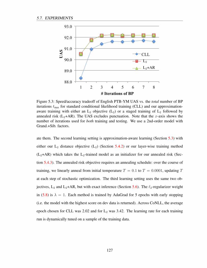
5.7. EXPERIMENTS
88.0
89.0
90.0
91.0
92.0
93.0
1 2 3 4 5 6 7 8
UA
S
# Iterations of BP
CLL
L2
L2+AR
Figure 5.3: Speed/accuracy tradeoff of English PTB-YM UAS vs. the total number of BPiterations tmax for standard conditional likelihood training (CLL) and our approximation-aware training with either an L2 objective (L2) or a staged training of L2 followed byannealed risk (L2+AR). The UAS excludes punctuation. Note that the x-axis shows thenumber of iterations used for both training and testing. We use a 2nd-order model withGrand.+Sib. factors.
ate them. The second learning setting is approximation-aware learning (Section 5.3) with
either our L2 distance objective (L2) (Section 5.4.2) or our layer-wise training method
(L2+AR) which takes the L2-trained model as an initializer for our annealed risk (Sec-
tion 5.4.3). The annealed risk objective requires an annealing schedule: over the course of
training, we linearly anneal from initial temperature T = 0.1 to T = 0.0001, updating T
at each step of stochastic optimization. The third learning setting uses the same two ob-
jectives, L2 and L2+AR, but with exact inference (Section 5.6). The ℓ2-regularizer weight
in (5.8) is λ = 1. Each method is trained by AdaGrad for 5 epochs with early stopping
(i.e. the model with the highest score on dev data is returned). Across CoNLL, the average
epoch chosen for CLL was 2.02 and for L2 was 3.42. The learning rate for each training
run is dynamically tuned on a sample of the training data.
127

5.7. EXPERIMENTS
90.5
91
91.5
92
92.5
Unary Grand. Sib. Grand.+Sib.
UA
S
CLL
L2
L2+AR
Figure 5.4: English PTB-YM UAS vs. the types of 2nd-order factors included in the modelfor approximation-aware training and standard conditional likelihood training. The UASexcludes punctuation. All models include 1st-order factors (Unary). The 2nd-order modelsinclude grandparents (Grand.), arbitrary siblings (Sib.), or both (Grand.+Sib.)—and use 4iterations of BP. For each of these models, the improvement given by training with ourmethod instead of CLL is statistically significant at the p < 0.005 level.
5.7.2 Results
Our goal is to demonstrate that our approximation-aware training method leads to im-
proved parser accuracy as compared with the standard training approach of conditional
log-likelihood (CLL) maximization (Smith and Eisner, 2008), which does not take inex-
act inference into account. The two key findings of our experiments are that our learning
approach is more robust to (1) decreasing the number of iterations of BP and (2) adding
additional cycles to the factor graph in the form of higher-order factors. In short: our
approach leads to faster inference and creates opportunities for more accurate parsers.
Speed-Accuracy Tradeoff Our first experiment is on English dependencies. For English
PTB-YM, Figure 5.3 shows accuracy as a function of the number of BP iterations for our
second-order model with both arbitrary sibling and grandparent factors on English. We find
that our training methods (L2 and L2+AR) obtain higher accuracy than standard training
(CLL), particularly when a small number of BP iterations are used and the inference is
128

5.7. EXPERIMENTS
a worse approximation. Notice that with just two iterations of BP, the parsers trained by
our approach obtain accuracy greater than or equal to those by CLL with any number of
iterations (1 to 8). Contrasting the two objectives for our approximation-aware training, we
find that our simple L2 objective performs very well. In fact, in only two cases, at 3 and 5
iterations, does risk annealing (L2+AR) further improve performance on test data. In our
development experiments, we also evaluated AR without using L2 for initialization and we
found that it performed worse than either of CLL and L2 alone. That AR performs only
slightly better than L2 (and not worse) in the case of L2+AR is likely due to early stopping
on dev data, which guards against selecting a worse model.
Increasingly Cyclic Models Figure 5.4 contrasts accuracy with the type of 2nd-order
factors (grandparent, sibling, or both) included in the model for English, for a fixed bud-
get of 4 BP iterations. Adding higher-order factors introduces more loops, making the
loopy BP approximation more problematic for standard CLL training. By contrast, under
approximation-aware training, enriching the model with more factors always helps perfor-
mance, as desired, rather than hurting it.
The UAS improvements given by our training method over CLL are significant at the
p < 0.005 level for each model we considered in Figure 5.4. The UAS for Sib. and
Grand.+Sib. with CLL training are statistically indistinguishable in Figure 5.4, despite the
noticeable drop. However, with approximation-aware training, the improvement from Sib.
to Grand.+Sib. is significant with p = 0.006.
Notice that our advantage is not restricted to the case of loopy graphs. Even when
we use a 1st-order model, for which BP inference is exact, our approach yields higher-
accuracy parsers than CLL training. We speculate that this improvement is due to our
method’s ability to better deal with model misspecification—a first-order model is quite
misspecified! Note the following subtle point: when inference is exact, the CLL estimator
is actually a special case of our approximation-aware learner—that is, CLL computes the
129

5.7. EXPERIMENTS
TRAIN INFERENCE DEV UAS TEST UASCLL Exact 91.99 91.62CLL BP 4 iters 91.37 91.25L2 Exact 91.91 91.66L2 BP 4 iters 91.83 91.63
Table 5.2: The impact of exact vs. approximate inference on a 2nd-order model withgrandparent factors only. Results are for the development (§ 22) and test (§ 23) sections ofPTB-YM.
same gradient that our training by backpropagation would if we used log-likelihood as the
objective.
Exact Inference with Grandparents Section 5.2 noted that since we always do MBR
decoding, the ideal strategy is to fit the true distribution with a good model. Consider
a “good model” that includes unary and grandparent factors. Exact inference is possible
here in O(n4) time by dynamic programming (Koo and Collins, 2010, Model 0). Table
5.2 shows that CLL training with exact inference indeed does well on test data—but that
accuracy falls if we substitute fast approximate inference (4 iterations of BP). Our pro-
posed L2 training is able to close the gap, just as intended. That is, we succesfully train
a few iterations of an approximate O(n3) algorithm to behave as well as an exact O(n4)
algorithm.
Other Languages Our final experiments train and test our parsers on 19 languages from
CoNLL-2006/2007 (Table 5.3). We find that, on average across languages, approximation-
aware training with an L2 objective obtains higher UAS than CLL training. This result holds
for both our poorest model (1st-order) and our richest one (2nd-order with grandparent and
sibling factors), using 1, 2, 4, or 8 iterations of BP. Figure 5.5 presents the results of Table
5.3 visually. Notice that the approximation-aware training doesn’t always outperform CLL
training—only in the aggregate. Again, we see the trend that our training approach yields
larger gains when BP is restricted to a small number of maximum iterations. It is possible
that larger training sets would also favor our approach, by providing a clearer signal of how
130
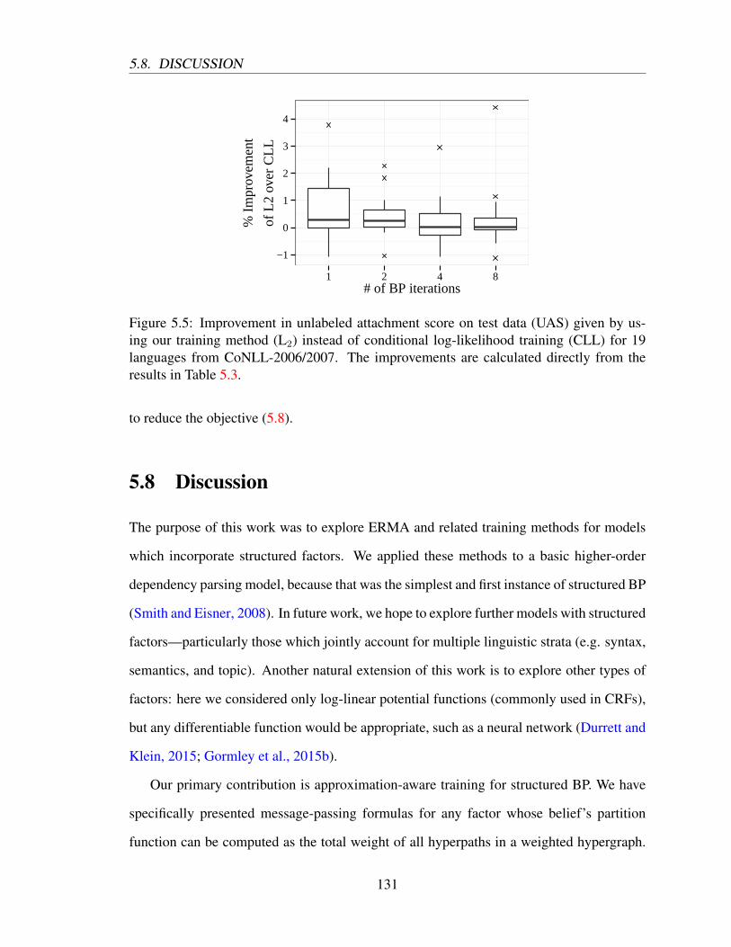
5.8. DISCUSSION
−1
0
1
2
3
4
1 2 4 8# of BP iterations
% Im
prov
emen
t
of L
2 ov
er C
LL
Figure 5.5: Improvement in unlabeled attachment score on test data (UAS) given by us-ing our training method (L2) instead of conditional log-likelihood training (CLL) for 19languages from CoNLL-2006/2007. The improvements are calculated directly from theresults in Table 5.3.
to reduce the objective (5.8).
5.8 Discussion
The purpose of this work was to explore ERMA and related training methods for models
which incorporate structured factors. We applied these methods to a basic higher-order
dependency parsing model, because that was the simplest and first instance of structured BP
(Smith and Eisner, 2008). In future work, we hope to explore further models with structured
factors—particularly those which jointly account for multiple linguistic strata (e.g. syntax,
semantics, and topic). Another natural extension of this work is to explore other types of
factors: here we considered only log-linear potential functions (commonly used in CRFs),
but any differentiable function would be appropriate, such as a neural network (Durrett and
Klein, 2015; Gormley et al., 2015b).
Our primary contribution is approximation-aware training for structured BP. We have
specifically presented message-passing formulas for any factor whose belief’s partition
function can be computed as the total weight of all hyperpaths in a weighted hypergraph.
131

5.8. DISCUSSION
1ST-
OR
DE
R2N
D-O
RD
ER
(WIT
HG
IVE
NN
UM
.B
PIT
ER
AT
ION
S)
12
48
LA
NG
UA
GE
CL
LL2−
CL
LC
LL
L2−
CL
LC
LL
L2−
CL
LC
LL
L2−
CL
LC
LL
L2−
CL
L
AR
77.6
3-0
.26
73.3
9+2
.21
77.0
5-0
.17
77.2
0+0
.02
77.1
6-0
.07
BG
90.3
8-0
.76
89.1
8-0
.45
90.4
4+0
.04
90.7
3+0
.25
90.6
3-0
.19
CA
90.4
7+0
.30
88.9
0+0
.17
90.7
9+0
.38
91.2
1+0
.78
91.4
9+0
.66
CS
84.6
9-0
.07
79.9
2+3
.78
82.0
8+2
.27
83.0
2+2
.94
81.6
0+4
.42
DA
87.1
5-0
.12
86.3
1-1
.07
87.4
1+0
.03
87.6
5-0
.11
87.6
8-0
.10
DE
88.5
5+0
.81
88.0
60.
0089
.27
+0.4
689
.85
-0.0
589
.87
-0.0
7E
L82
.43
-0.5
480
.02
+0.2
981
.97
+0.0
982
.49
-0.1
682
.66
-0.0
4E
N88
.31
+0.3
285
.53
+1.4
487
.67
+1.8
288
.63
+1.1
488
.85
+0.9
6E
S81
.49
-0.0
979
.08
-0.3
780
.73
+0.1
481
.75
-0.6
681
.52
+0.0
2E
U73
.69
+0.1
171
.45
+0.8
574
.16
+0.2
474
.92
-0.3
274
.94
-0.3
8H
U78
.79
-0.5
276
.46
+1.2
479
.10
+0.0
379
.07
+0.6
079
.28
+0.3
1IT
84.7
5+0
.32
84.1
4+0
.04
85.1
5+0
.01
85.6
6-0
.51
85.8
1-0
.59
JA93
.54
+0.1
993
.01
+0.4
493
.71
-0.1
093
.75
-0.2
693
.47
+0.0
7N
L76
.96
+0.5
374
.23
+2.0
877
.12
+0.5
378
.03
-0.2
777
.83
-0.0
9P
T86
.31
+0.3
885
.68
-0.0
187
.01
+0.2
987
.34
+0.0
887
.30
+0.1
7S
L79
.89
+0.3
078
.42
+1.5
079
.56
+1.0
280
.91
+0.0
380
.80
+0.3
4S
V87
.22
+0.6
086
.14
-0.0
287
.68
+0.7
488
.01
+0.4
187
.87
+0.3
7T
R78
.53
-0.3
077
.43
-0.6
478
.51
-1.0
478
.80
-1.0
678
.91
-1.1
3Z
H84
.93
-0.3
982
.62
+1.4
384
.27
+0.9
584
.79
+0.6
884
.77
+1.1
4A
VG
.83
.98
+0.0
482
.10
+0.6
883
.88
+0.4
184
.41
+0.1
984
.34
+0.3
1
Tabl
e5.
3:R
esul
tson
19la
ngua
ges
from
CoN
LL
-200
6/20
07.
For
lang
uage
sap
pear
ing
inbo
thda
tase
ts,
the
2006
vers
ion
was
used
,ex
cept
forC
hine
se(Z
H).
We
repo
rtab
solu
teU
AS
fort
heba
selin
e(C
LL
)and
the
impr
ovem
enti
nU
AS
forL
2ov
erC
LL
(L2−
CL
L)w
ithpo
sitiv
e/ne
gativ
edi
ffer
ence
sin
blue
/red
.The
UA
Sin
clud
espu
nctu
atio
n.T
heav
erag
eU
AS
and
aver
age
diff
eren
ceac
ross
alll
angu
ages
(AV
G.)
isgi
ven.
Diff
eren
ces
(bet
ter/
wor
se)
inbo
ldar
est
atis
tical
lysi
gnifi
cant
atth
ep<
0.05
leve
l.T
hese
resu
ltsar
efu
rthe
ran
alyz
edin
Figu
re5.
5.
132

5.9. SUMMARY
This would suffice to train the structured BP systems that have been built for projective
dependency parsing (Smith and Eisner, 2008), CNF grammar parsing (Naradowsky et al.,
2012b), TAG (Auli and Lopez, 2011), ITG-constraints for phrase extraction (Burkett and
Klein, 2012), and graphical models over strings (Dreyer and Eisner, 2009).
5.9 Summary
We introduce a new approximation-aware learning framework for belief propagation with
structured factors. We present differentiable objectives for both empirical risk minimization
(a la ERMA) and a novel objective based on L2 distance between the inferred beliefs and the
true edge indicator functions. Experiments on the English Penn Treebank and 19 languages
from CoNLL-2006/2007 shows that our estimator is able to train more accurate dependency
parsers with fewer iterations of belief propagation than standard conditional log-likelihood
training, by taking approximations into account.
133

Chapter 6
Graphical Models with Structured and
Neural Factors and
Approximation-aware Learning
The previous chapters have illustrated three key points: (1) latent variables are an effective
modeling tool that can outperform some grammar induction systems (Chapter 3), (2) both
traditional hand-crafted features and learned features can be treated as factors in a factor
graph (Chapter 4), and (3) for structured graphical models with cycles, approximation-
aware training can yield faster and more accurate systems (Chapter 5).
In this chapter, we combine the methods from the previous three chapters in order to
obtain the benefits of them all. We propose graphical models with structured factors, neural
factors, and approximation-aware training in a semi-supervised setting. Following our orig-
inal motivation, we focus here on a low-resource setting for semantic role labeling where a
joint model with latent dependency and tagging syntax improves our overall performance.
134

6.1. INTRODUCTION
6.1 Introduction
Many tasks in NLP focus on a single linguistic stratum when in fact we care about several.
The reasons for this are often practical: machine learning does not provide the tools that
allow one to readily create a joint model of multiple levels of linguistic data.
The types of models we hope to build would elegantly handle low-resource settings,
taking advantage of whatever data is available. Though fully unsupervised methods (e.g.
(Smith, 2006; Spitkovsky, 2013)) provide one option, they are not catered to a specific
task and a small amount of supervision can often outperform them (Naseem et al., 2010;
Søgaard, 2012). For the task of semantic role labeling (SRL), it is difficult to say whether
joint modeling is worth the extra effort when supervised training data abounds.1 However,
in low-resource settings, the advantages of joint modeling are clearer (Boxwell et al., 2011;
Naradowsky et al., 2012a; Gormley et al., 2014) (Chapter 3).
Because our focus is on NLP, we seek to build models that allow declarative constraints
to be specified over a set of variables. This arises in many tasks such as dependency parsing
(Riedel and Clarke, 2006; Smith and Eisner, 2008; Martins et al., 2009), constituency
parsing (Naradowsky et al., 2012b), phrase extraction (Burkett and Klein, 2012), TAG (Auli
and Lopez, 2011), and SRL (Das et al., 2012). Dual decomposition and other techniques
allow for MAP inference in these sorts of models (Duchi et al., 2006; Riedel and Clarke,
2006; Martins et al., 2009; Koo et al., 2010; Martins et al., 2011b). However, because of
our interest in low-resource settings we expect that it will be useful to marginalize over
the unobserved variables in our model—so we turn to marginal inference by structured BP
(Smith and Eisner, 2008).
These inexact inference techniques can cause problems for standard learning algorithms
(Kulesza and Pereira, 2008). For MAP inference there exist algorithms that can handle this
inexact inference (Huang et al., 2012; Zhang et al., 2013). But for marginal inference the
1The top performers in the CoNLL-2009 shared task (Gesmundo et al., 2009; Hajic et al., 2009; Lluıset al., 2013) for joint syntactic and semantic dependency parsing provide evidence of this.
135

6.1. INTRODUCTION
existing algorithms can’t handle structured factors (Stoyanov et al., 2011; Domke, 2011).
Finally, a variety of work old (Bengio et al., 1990; Bengio et al., 1992; Haffner, 1993;
Bengio and Frasconi, 1995; Bengio et al., 1995; Bourlard et al., 1995) and new (Ning et
al., 2005; Morin and Bengio, 2005; Do and Artieres, 2010; Tompson et al., 2014; Srikumar
and Manning, 2014) has explored hybrids of graphical models and neural networks for
structured prediction. Applications of these techniques have included SRL (Collobert and
Weston, 2008; Foland and Martin, 2015; FitzGerald et al., 2015). However, none of this
work handles the case of structured factors, latent variables, neural factors, and inexact
inference that we are concerned with here.
In this chapter we introduce a framework that permits (a) structural constraints over
latent variables, (b) learned features, (c) efficient approximate inference, and (d) learning
that performs well despite any approximations made by our system. We demonstrate its
effectiveness on the task of low-resource semantic role labeling. The introduction of this
framework is at the core of the contributions of this chapter:
• We introduce a new variety of hybrid graphical models and neural networks.
• We propose approximation-aware training for structured belief propagation with neu-
ral factors.
• We unify three forms of inference: BP on factor graphs, inside-outside on a hyper-
graph, and feed-forward computation in a neural network.
• We introduce a joint model of this type for semantic role labeling, syntactic depen-
dency parsing, and part-of-speech tagging.
• We study this model in a low-resource setting for SRL that treats the syntax (parse
and tags) as latent and trains in a semi-supervised fashion.
We begin by introducing a novel graphical model with structured and neural factors (Sec-
tion 6.2). Taking a probabilistic perspective of the model, we describe how to carry out
136
6.2. MODEL
approximate inference (Section 6.3), decoding (Section 6.4), and approximation-unaware
surrogate likelihood training (Section 6.5.1). Finally, we train the same system to be
approximation-aware (Section 6.5.2). Doing so leads to an alternative perspective of our
model as a deep neural network whose topology is inspired by approximate inference on
the graphical model of this section.
6.2 Model
We introduce a model for joint semantic role labeling, syntactic dependency parsing, and
part-of-speech tagging. Note however that we will use this model in a semi-supervised
setting: during training, we will observe semantic roles for each sentence, but not syntactic
dependencies or part-of-speech tags—the same low-resource setting as Chapter 3. Accord-
ingly, the syntax will be treated as latent and will only act in the service of our semantic
role labeler.
Semantic Role Labeler Our semantic role labeler is a conditional model pθ(r | x),
which is defined by marginalizing our joint model for syntax and semantics pθ(r, e, t | x).
For the conditional model, the input x is a sentence. An output assignment r encodes a
semantic role labeling of the sentence. The latent structure {e, t} consists of a syntactic de-
pendency tree e and a part-of-speech tagging t. The probability of a semantic role labeling
r for a given sentence x can thus be written in form:
pθ(r | x) =∑
e,t
pθ(r, e, t | x) (6.1)
This distribution defines the probability of the output variables R given the input variables
X , marginalizing over the latent variables {E,T }. The form of the joint model pθ(r, e, t |
x) is discussed below.
137

6.2. MODEL
Joint Model of Syntax and Semantics Our joint model pθ(r, e, t | x) defines the prob-
ability of the semantics r and latent syntax {e, t} given the sentence x. We will describe
this joint model as a factor graph (Frey et al., 1997; Kschischang et al., 2001). We fol-
low our definition of factor graphs given in Section 2.3.1. For conciseness, we abbreviate
the full set of output variables for the joint model as Y = {R,E,T }. The probability is
proportional to a product of non-negative potential functions ψα:
pθ(r, e, t | x) = pθ(y | x) = 1
Z(x)
∏
α
ψα(yαx) (6.2)
where Z(x) is the sentence-specific partition function ensuring that the distribution sums
to one. One of the main contributions of this chapter is that the potential functions (which
are in one-to-one correspondence with factors α) come in one of three forms:
Log-linear factors These constitute the standard potential function for a conditional
random field (CRF) (Lafferty et al., 2001) having the form ψα(yα) = exp(θ ·
fα(yα,x)). In our model, we define a log-linear factor for each variable. How-
ever, we also include factors over pairs of variables. These connect the depen-
dency edge variables E to the roles R, and the tag variables T to the roles R.
Neural factors Potential functions for these factors are defined by the score of an FCM
neural network from Section 4.3. While these neural factors would be appropriate
for all the variables, we only include them as unary factors on the semantic roles
R, since they are more computationally intensive during inference and learning
than the log-linear factors.
Structured factors We include only one structured factor, PTREE, which constrains
the syntactic dependency variables E to form a projective tree. See Section 2.3.3.4
for a detailed description of the form of this factor.
Figure 6.1 depicts the factor graph for a short sentence. The factor graph for our joint
138

6.3. INFERENCE
model has elements of those given earlier in this thesis: The model of syntactic/semantic
dependencies is akin to our models from Section 3.2.3 and Section 5.2. The combination
of exponential family factors and the neural network FCM factors is similar to those used
in our relation extraction model from Section 4.5.
6.3 Inference
The goal of marginal inference is to compute or approximate the variable and factor marginals
(reiterated from equation (2.16) and equation (2.17)):
pθ(yi | x) =∑
y′:y′i=yi
pθ(y′ | x) (6.3)
pθ(yα | x) =∑
y′:y′α=yα
pθ(y′ | x) (6.4)
and the partition function (reiterated from equation (2.9)):
Z(x) =∑
y
∏
α
ψα(yα,x) (6.5)
Exact inference in our model is intractable due to high treewidth of the factor graph. How-
ever, we can carry out approximate marginal inference by structured loopy belief propaga-
tion (BP) (Smith and Eisner, 2008). For a detailed discussion of this algorithm, we refer the
reader to Section 2.3.3.4, Section 5.2, and Section 5.5.3. Here, we highlight the important
characteristics of applying this algorithm to our model.
Structured BP is a message passing algorithm, where each message takes the form of
a (possibly unnormalized) distribution over a single variable in the factor graph. Messages
from structured factors (i.e. those with a large set of neighboring variables) are computed
by variants of familiar dynamic programming algorithms—for our model the PTREE factor
uses a variant of the inside-outside algorithm of Eisner (1996). The other messages are
139

6.3. INFERENCE
0 2 1 3 4 Marta the stole ball $
R2,1
E2,1
R1,2
E1,2
R3,2
E3,2
R2,3
E2,3 R3,1
E3,1
R1,3
E1,3
R4,3
E4,3
R3,4
E3,4 R4,2
E4,2
R2,4
E2,4 R4,1
E4,1
R1,4
E1,4
E0,1
E0,3
E0,4
E0,2
T1 T2 T3 T4
Figure 6.1: Factor graph for joint semantic and syntactic dependency parsing and syntactictagging of a 4-word sentence; $ is the root of the dependency graph. The semantic rolevariable Rp,a (yellow) encodes whether and what type of role holds between a predicatep and an argument a. The boolean variable Eh,m (blue) encodes whether the syntacticdependency edge from head h to modifier m is present. The tag variable Ti gives the part-of-speech tag for word i. The structured PTREE factor (red) coordinates all the syntacticdependency variables to ensure that the edges form a tree. Each unary FCM factor (green)scores a semantic role variable using a neural network. The remaining factors (black) scoreone or more variables according to a log-linear function using hand-crafted features. Thesimplest of these are unary and score each variable in isolation. The binary factors betweensemantic role and syntactic dependency variables score the syntax/semantics interface. Thebinary factors between pairs of tag variables score tag bigrams. The drawing shows a fewfactors between the semantic role variables and the tag variables. Note that the combinationof all these factors yields a cyclic (“loopy”) graph.
140

6.4. DECODING
easily computed with standard tensor operations—these include messages from our log-
linear factors and neural factors. These message computations are local in that they only
look at the incoming messages and, for messages from factors, one potential function.
On acyclic graphs (examples include our SRL and relation extraction models from
Chapter 3 and Chapter 4), this algorithm performs exact marginal inference. On cyclic
graphs (i.e. those with loops), such as our joint model (Section 6.2), the algorithm per-
forms approximate inference by ignoring the loops. It terminates either at convergence or
after a fixed number of iterations. The outputs of BP are beliefs (i.e. approximate variable
and factor marginals). The objective functions we consider for training (Section 6.5) will
rely on these beliefs.
6.4 Decoding
To facilitate comparison with prior work and to evaluate our models, we wish to obtain a
single assignment to the output variables. For the semantic role labeling task we consider in
Section 6.6, our true loss function is F1 score: the harmonic mean of precision and recall for
the semantic role variables R. A minimum Bayes risk (MBR) decoder for this task should
take this loss function into account. However, doing so is not straightforward because
the loss function doesn’t decompose over the factors—by contrast, it is coupled across
sentences. For simplicity, we instead use the MBR decoder for Hamming loss (reiterated
from equation (2.15)):
ri = hθ(x)i = argmaxri
pθ(ri | x) (6.6)
This same decoder was employed in Chapter 3 for SRL and Chapter 4 for relation extrac-
tion. In Chapter 5, we also used an MBR decoder for parsing with a constraint that the
output variables formed a tree.
141
6.5. LEARNING
6.5 Learning
The training data for SRL in the low-resource setting consist of a dataset of pairs {x(d), r(d)}Dd=1
where x(d) is a sentence, and r(d) a role labeling. We do not observe either a syntactic de-
pendency parse e or a tagging t. The goal of learning is to find model parameters θ which
yield a decision function hθ(x) whose predictions give low loss on the unobserved test
sentences. As in Section 5.3, we minimize an ℓ2-regularized objective function:
θ∗ = argminθ
1
D
(( D∑
d=1
J(θ;x(d), r(d)))+λ
2||θ||22
)(6.7)
where λ > 0 is the regularization coefficient and J(θ;x, r∗) is a given differentiable ob-
jective function. Our model parameters θ consist of all those needed for the log-linear and
neural factors in our model.
6.5.1 Approximation-Unaware Training
The standard approach to training a graphical model is conditional log-likelihood maxi-
mization. We can also apply this technique to our graphical model with structured and
neural factors. We set J(θ;x, r∗) = log pθ(r | x) in order to maximize the marginal like-
lihood in equation (6.1). This log-likelihood is computed as the difference of two partition
functions (see Section 2.3.4.1 for details). We can approximate those partition functions
using the Bethe Free Energy (see Section 2.3.3.3 for an explanation) which is a simple
function of the beliefs output by Structured BP, given in equation (2.27).
Section 2.3.4.1 describes how to compute the gradient of this marginal log-likelihood
objective when all of the factors are log-linear. This is not the case in our model, because we
include neural factors. Instead, we compute the partial derivatives of the conditional log-
likelihood pθ(r|x) with respect to the log potential functions logψα(yα). These partials
require the true factor marginals, but we replace them with the final beliefs from structured
BP. Finally, we backpropagate from these partials through the factors to the model pa-
142

6.5. LEARNING
rameters. This gives the gradient of the surrogate marginal log-likelihood, the marginal
variant of Wainwright (2006)’s surrogate likelihood. This is akin to the surrogate likeli-
hood objective we considered in Section 5.6, yet there we did not marginalize out any of
the variables.
For some of the models we will consider, structured BP computes the true marginals,
in which case we are maximizing the conditional marginal log-likelihood.
6.5.2 Approximation-Aware Training
The surrogate likelihood training described above may perform poorly when the inference
approximation is poor. Here, we instead consider training in an approximation-aware fash-
ion. Following Section 5.3 we could treat our entire system (inference, decoding, loss) as
a differentiable circuit and minimize the regularized empirical risk. We take the simpler
approach of minimizing the L2 distance objective presented in Section 5.4.2 which does
not incorporate the decoder or (true) loss function into the system during backpropagation
training. That is, we set J(θ;x, r∗) =∑
i
∑ri(bi(ri) − b∗i (ri))
2, where the L2 distance is
computed only over the semantic role labeling variables R observed during training.
In Section 6.3, we used a probabilistic definition of inference for our graphical model
(i.e. two of the three inference tasks from Section 2.3.3). By contrast, inference in a
neural network amounts to a straightforward feedforward computation (see examples in
Section 2.2) that might have no probabilistic interpretation. By training our approximation-
aware model, we have effectively defined a new deep neural network, where inference is
a feed-forward computation. Note however, that in our deep network, this feed-forward
computation incorporates several iterations of BP and any embedded dynamic program-
ming algorithms used to compute messages from structured factors. In this way, inference
could be said to have no probabilistic interpretation (we gave this up as soon as we chose
to do approximate inference by BP!). However, our inference procedure provides a unified
method of combining BP on a factor graph, dynamic programming on a hypergraph, and
143

6.6. EXPERIMENTS
the feed-forward computation of a neural network. The goal of training is therefore to tune
the parameters so that these algorithms perform well in concert with each other.
6.6 Experiments
The goal of our experiments is to explore the merits of graphical models with structured
factors, neural factors, and approximation-aware training. To that end, we consider the task
of low-resource SRL.
6.6.1 Experimental Setup
Data We consider five languages from the CoNLL-2009 Shared Task (Hajic et al., 2009):
Catalan, Czech, German, English, and Spanish. In order to simulate a low-resource setting,
for each language, we use only the first 1000 sentences from the training set and discard the
rest. We use the standard development and test sets. We also remove all the supervised or
automatically annotated data (e.g. lemmas, part-of-speech tags, morphology, dependency
trees) except for the words and the semantic roles. Note that our use of the full development
set is somewhat artificial for the low-resource setting since its size for most languages is
comparable to the training set size. However, using this dev set allows us to carefully
regularize our models by early stopping (see below)—thereby improving the stability of
our results.
Evaluation Metrics Following the standard evaluation for the shared task, we report
Precision, Recall, and F1 on the test set. Each of these can be computed for two settings:
unlabeled and labeled. The unlabeled case assesses whether the correct arguments were
identified. The labeled case further asks whether the argument was given the correct role
label (arg0, arg1, argM, etc.). Regardless of the evaluation method, we always train on the
full labeled training set. These quantities are computed by the standard evaluation script
144

6.6. EXPERIMENTS
from the shared task.
Hyperparameters The learning rate is selected automatically on a subsample of the
training data. The embeddings are rescaled so that ||e||2 = 1. The weight of the ℓ2-
regularizer is λ = 1. We also regularize by early stopping; that is we select the model with
the highest labeled F1 on the development set, checking at the end of each epoch.
Models We consider a sequence of models, starting with a baseline and additively build-
ing up to our full model.
(A) Our baseline SRL model consisting only of the semantic role labeling variables
R with unary log-linear factors. This is the SRL-only model from Section 3.2.1.3
and Gormley et al. (2014).
(B) We next add the latent syntactic dependency edge variables E and the binary
factors connecting them to the role variables R.
(C) This model additionally includes the structured factor, PTREE, which constrains
the dependency edge variables E to form a tree. This is the joint SRL model from
Section 3.2.3 and Gormley et al. (2014).
(D) Next we add the latent tag variables T and the factors connecting them to the
role variables R. This is our first cyclic (“loopy”) model. We run BP for only
4 iterations using the same message passing schedule described in footnote 6 of
Section 5.2.
(E) We then add the neural factors which score the role variables R according to a
log-linear FCM submodel.
(F) Finally, we allow for fine-tuning of the word embeddings, thereby replacing the
log-linear FCM submodel with its log-bilinear equivalent.
145

6.6. EXPERIMENTS
(D), (E), (F) For each loopy model above we also consider the variant trained with
approximation-aware learning to maximize the L2 distance objective function. (F)
constitutes our full model.
Features The feature set we use for the unary and binary log-linear factors on the role R
and parse E variables are identical to those described in Section 3.4.2 for the low-resource
setting (there they are denoted by IGC). We do the same feature selection by information
gain described in Section 3.2.6.
For the FCM factors we use a feature set that is similar to those given for relation ex-
traction in Table 4.2: In place of the heads of first and second named entity, we consider the
predicate and argument heads. In place of the named entity types, we use a brown cluster
cutoff to length 4. We consider fewer in-between features: only those up to a maximum of
4 words away from either the predicate or argument heads. Since we do not observe any
dependency trees, we do not include the on-path features.
6.6.2 Results
Additive Experiment Our main results, presented in Table 6.1, are an additive exper-
iment on five CoNLL-2009 languages. We compare labeled (Table 6.1b) and unlabeled
(Table 6.1a) F1 for 7 models from the sequence of models described in Section 6.6.1. Our
aim is to better understand the contributions of different aspects of the full model (F). We
highlight two baselines from among this sequence: The ‘SRL unary only’ baseline (A) is
the semantics-only model from Section 3.2.1.3. The row ‘+PTREE factor’ (C) corresponds
to our joint syntax-semantics model from Section 3.2.3.
Adding the latent syntax tree variables T , the PTREE factor, the FCM factor, and
approximation-aware training all improve performance. The biggest average gain (+14.82)
is given by the addition of the structured factor. Two additions to the model hurt average
F1: the addition of the latent tag variables T and the incorporation of fine-tuning. The
146

6.6. EXPERIMENTS
Unlabeled F1ca cs de en es Avg. Avg. Diff.
(A) SRL unary only 42.42 39.26 18.37 46.75 44.12 38.18 –(B) +latent tree vars 45.55 45.73 18.79 47.33 47.16 40.91 +2.73(C) +PTREE factor 65.51 56.23 31.79 59.01 66.11 55.73 +14.82(D) +latent tag vars 66.55 57.09 25.37 59.45 66.56 55.00 -0.73(E) +FCM factors 70.08 63.79 34.63 63.23 70.04 60.35 +5.35(E) +approx.-aware 70.03 61.95 39.78 63.43 72.52 61.54 +1.19(F) +fine tuning 66.95 57.90 38.13 63.20 69.69 59.17 -2.37
(a)
Labeled F1ca cs de en es Avg. Avg. Diff.
(A) SRL unary only 31.99 33.65 13.38 39.56 32.20 30.16 –(B) +latent tree vars 33.95 38.26 13.54 39.80 33.83 31.88 +1.72(C) +PTREE factor 44.89 43.04 20.95 46.70 44.30 39.98 +8.10(D) +latent tag vars 45.42 43.49 18.28 47.51 44.95 39.93 -0.05(E) +FCM factors 49.86 50.90 24.57 51.36 50.36 45.41 +5.48(E) +approx.-aware 50.38 47.72 28.37 52.94 51.86 46.25 +0.84(F) +fine tuning 47.85 43.65 27.43 50.46 49.40 43.76 -2.50
(b)
Table 6.1: Additive experiment for five languages from CoNLL-2009: Catalan (ca), Czech(cs), German (de), English (en), and Spanish (es). Results on both unlabeled (a) and labeled(b) F1 are shown. We also include the average F1 (Avg.) and the average difference in F1for each model and the one above it (Avg. Diff.). Details of the models are given inSection 6.6.1.
bulk of the drop in performance when adding the latent tags comes from the German (de)
language setting, the annotations for which are very sparse. It seems reasonable that fine
tuning would cause the model to overfit—however both the train and dev F1 go down when
adding fine tuning. Because the learning rate is automatically selected and we only run for
a fixed number of epochs, the lack of overfitting may be evidence that training did not con-
verge. On average, our best model (E) (in both labeled and unlabeled F1) is obtained by
combining all of the ingredients except for fine-tuning.
Precision and Recall on English While our discussion above focused on F1, we also
considered the performance of the same sequence of models on precision and recall. Fig-
147

6.6. EXPERIMENTS
ca de en es Avg.CLL L2 − CLL CLL L2 − CLL CLL L2 − CLL CLL L2 − CLL CLL L2 − CLL
(D) all latent 66.55 -1.77 25.37 +11.22 59.45 -1.89 66.56 -1.09 54.48 +1.62(E) +FCM factors 70.08 -0.05 34.63 +5.15 63.23 +0.20 70.04 +2.48 59.50 +1.95(F) +fine tuning 68.70 -1.75 23.64 +14.49 61.30 +1.90 68.43 +1.26 55.52 +3.98
(a) Unlabeled F1.
ca de en es Avg.CLL L2 − CLL CLL L2 − CLL CLL L2 − CLL CLL L2 − CLL CLL L2 − CLL
(D) all latent 45.42 +0.23 18.28 +5.74 47.51 -1.07 44.95 +0.24 39.93 +0.86(E) + FCM factors 49.86 +0.52 24.57 +3.80 51.36 +1.58 50.36 +1.50 60.35 +1.19(F) +fine tuning 47.62 +0.23 17.09 +10.34 49.48 +0.98 48.53 +0.87 40.68 +3.08
(b) Labeled F1.
Table 6.2: Effect of approximation-aware learning. Results are show for both unlabeled(a) and labeled (b) F1. We report absolute F1 for the surrogate likelihood baseline (CLL)and the improvement in F1 for L2 over CLL (L2 − CLL) with positive/negative differences inblue/red.
ure 6.2 shows the results for English only. Observe that any increase of more than 0.5 in F1
is always accompanied by an improvement to both precision and recall. The precision is
fairly high for all the models and only improves slightly: our baseline (A) obtains precision
80.21 and it increases only to 86.74 with our best model (E). By contrast, recall remains
low for all of our models, though the increase is larger: the baseline performance of (A) at
32.99 increases to 50.00 for our best model (E).
Effects of Approximation-aware Learning Finally, we consider the effects of approximation-
aware learning on three different models. The first is our loopy model obtained by includ-
ing both latent parsing E and tagging T variables and the accompanying factors (D). The
second additionally includes the FCM factors on the role variables R (E). The third adds
fine-tuning of the word embeddings (F). We contrast surrogate likelihood training (Sec-
tion 6.5.1) with training by backpropagation with the L2 distance objective (Section 6.5.2).
Training with the latter corresponds to the models (D), (E), and (F) described in Sec-
tion 6.6.1.
Table 6.2 presents our results on labeled and unlabeled F1. On average, L2 distance
training performs better across the four languages shown than surrogate likelihood training.
148

6.6. EXPERIMENTS
80.21 80.03 82.35 81.57 85.97 86.74 85.70
32.99 33.60
45.98 46.77 50.00 50.00 50.06
46.75 47.33
59.01 59.45 63.23 63.43 63.20
0.00
10.00
20.00
30.00
40.00
50.00
60.00
70.00
80.00
90.00
100.00
SRL unary
only
+laten
t tree
vars
+PTree fa
ctor
+laten
t tag v
ars
+FCM facto
rs
+appro
x.-aw
are
+fine t
uning
P
R
F1
Figure 6.2: Unlabeled precision (P), recall (R), and F1 for additive experiment on Englishdata from CoNLL-2009. The sequence of models and the F1 results are the same as that inTable 6.1a—the P/R results shown here are not given in the table.
149

6.6. EXPERIMENTS
However, for Catalan (ca), surrogate likelihood always performs better in unlabeled F1.
Further, for unlabeled F1, most of the gains in that average come from German (de). The
gains in labeled F1 are more stable. In all but one case, approximation-aware learning
outperforms the baseline.
6.6.3 Error Analysis
In this section, we attempt to isolate the contributions of specific model components on
English performance. Specifically, we focus on the two additions to the model that gave
the largest gains in F1 on English in our main results: the PTREE factor and the FCM
factors. We consider a set of four models:
1. New Baseline (NB): This model, trained with approximation-aware learning and
an L2-distance objective, contains the semantic and syntactic dependency vari-
ables, and their associated unary factors. It also includes binary factors connecting
each pair.
2. NB+PTREE: This model adds a PTREE factor to the New Baseline. Notice that
this new factor does not introduce any additional model parameters since it is a
purely declarative constraint over the latent syntactic variables.
3. NB+FCM: Next, we take the New Baseline and add the FCM factors. Table 6.3
shows that, unlike PTREE, the FCM factors introduce a very large number of model
parameters yielding a much higher capacity model.
4. NB+PTREE+FCM: Finally, we combine the PTREE factor and the FCM factors
into the New Baseline model.
The experiments in this section mirror the experimental setup described in Section 6.6.1,
except that we train on the first 5,000 sentences in the CoNLL-2009 English dataset. The
development and test sets remain the same. Table 6.3 presents the main results for this
150
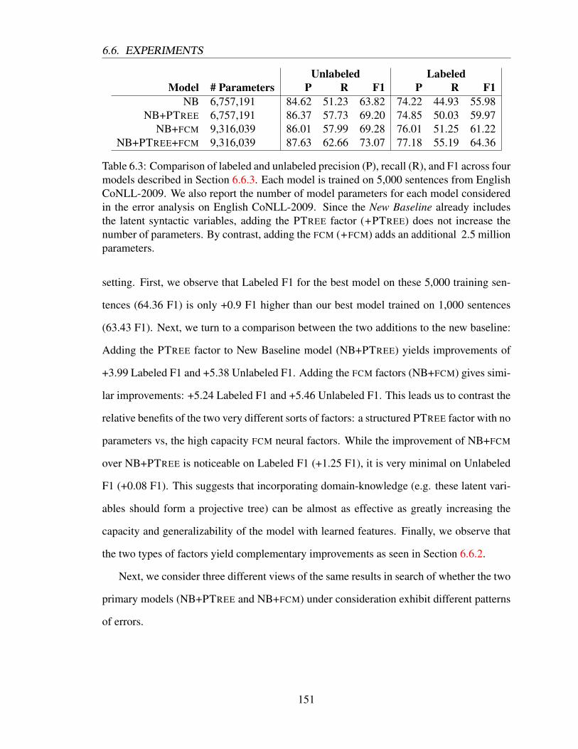
6.6. EXPERIMENTS
Unlabeled LabeledModel # Parameters P R F1 P R F1
NB 6,757,191 84.62 51.23 63.82 74.22 44.93 55.98NB+PTREE 6,757,191 86.37 57.73 69.20 74.85 50.03 59.97
NB+FCM 9,316,039 86.01 57.99 69.28 76.01 51.25 61.22NB+PTREE+FCM 9,316,039 87.63 62.66 73.07 77.18 55.19 64.36
Table 6.3: Comparison of labeled and unlabeled precision (P), recall (R), and F1 across fourmodels described in Section 6.6.3. Each model is trained on 5,000 sentences from EnglishCoNLL-2009. We also report the number of model parameters for each model consideredin the error analysis on English CoNLL-2009. Since the New Baseline already includesthe latent syntactic variables, adding the PTREE factor (+PTREE) does not increase thenumber of parameters. By contrast, adding the FCM (+FCM) adds an additional 2.5 millionparameters.
setting. First, we observe that Labeled F1 for the best model on these 5,000 training sen-
tences (64.36 F1) is only +0.9 F1 higher than our best model trained on 1,000 sentences
(63.43 F1). Next, we turn to a comparison between the two additions to the new baseline:
Adding the PTREE factor to New Baseline model (NB+PTREE) yields improvements of
+3.99 Labeled F1 and +5.38 Unlabeled F1. Adding the FCM factors (NB+FCM) gives simi-
lar improvements: +5.24 Labeled F1 and +5.46 Unlabeled F1. This leads us to contrast the
relative benefits of the two very different sorts of factors: a structured PTREE factor with no
parameters vs, the high capacity FCM neural factors. While the improvement of NB+FCM
over NB+PTREE is noticeable on Labeled F1 (+1.25 F1), it is very minimal on Unlabeled
F1 (+0.08 F1). This suggests that incorporating domain-knowledge (e.g. these latent vari-
ables should form a projective tree) can be almost as effective as greatly increasing the
capacity and generalizability of the model with learned features. Finally, we observe that
the two types of factors yield complementary improvements as seen in Section 6.6.2.
Next, we consider three different views of the same results in search of whether the two
primary models (NB+PTREE and NB+FCM) under consideration exhibit different patterns
of errors.
151

6.6. EXPERIMENTS
0.00
10.00
20.00
30.00
40.00
50.00
60.00
70.00
80.00
90.00
1 2 3-6 7-...
F1
binned # of tokens separating predicate and argument
NB
NB+PTree
NB+FCM
NB+PTree+FCM
Figure 6.3: F1 of SRL for predicate-argument distance. We divide each possible predicate-argument pair into a bin based on the number of tokens separating the two heads: 1 token,2 tokens, 3 to 6 tokens apart, or 7 or more tokens. The F1 computation is restricted to onlythe semantic edges in the respective bin for the four models in Section 6.6.3.
Predicate-Argument Distance Next, we divide all the possible predicate-argument pairs
into bins by the number of tokens separating the predicate head and argument head. For
each bin, we compute the F1 score of each model on only the corresponding subset of
predicate-argument pairs. These results are summarized in Figure 6.3. The largest relative
improvements are found on longer dependencies (e.g. 3 to 6 tokens apart, and more than
7 tokens apart) for both NB+PTREE and NB+FCM. However, these relative improvements
also correspond to the settings which, without those added factors, were performing the
worst. The distribution of the gold predicate-argument pairs between the bins was fairly
even: 38.13% separated by 1 token, 23.74% by 2 tokens, 25.05% by 3-6, and 13.08% by 7
or more.
Nominal vs. Verbal Predicates We can also divide the predicate-argument pairs by the
(gold) part-of-speech tag for the predicate head. The full set of such Penn Treebank tags
when truncated to the first two characters includes CC, CD, IN, JJ, NN, PD, RP, VB, WP,
and WR. However, 99.70% of them are accounted for by the nominal (NN, 39.47%) and
verbal (VB, 60.23%) predicates. So we focus our discussion only on these two types of
predicates. Figure 6.4 gives the F1 results for our four models binning by whether the
152

6.6. EXPERIMENTS
50.00
52.00
54.00
56.00
58.00
60.00
62.00
64.00
66.00
68.00
Nominal Verbal
F1
NB
NB+PTree
NB+FCM
NB+PTree+FCM
Figure 6.4: F1 of SRL across nominal and verbal predicates. We bin the predicate-argumentpairs based on whether the predicate is nominal (has a gold POS tag starting with NN) orverbal (POS tag starting with VB). F1 is computed separately for each bin on each of thefour models in Section 6.6.3.
predicate was nominal or verbal.
Despite there being over 1.5 times as many verbal predicate-argument training exam-
ples, each model performs respectively better on nominal predicates than verbal. We find
that relative improvement of NB+FCM over NB+PTREE is much higher on the nominal
than verbal predicates.
Semantic Role Types Finally, we ask whether there are observable differences in the
relative improvements across role labels for the two types of factors. We again bin the
pairs, this time by the label of the predicate-argument pair. These post-hoc results are
akin to what we would observe if we trained a separate model for each role. One of the
smallest differences in the relative improvement given by +PTREE and +FCM is found in
the most frequently occurring role, A1, which usually corresponds to an Patient or Theme
role. The advantage of +FCM over +PTree seems particularly pronounced by the second
most common role, A0, which is often an Agent role.
153

6.7. SUMMARY
Role Label % of Gold NB NB+PTREE NB+FCM NB+PTREE+FCM
A1 37.06% 59.21 64.05 64.75 68.44A0 25.15% 60.41 63.35 64.90 67.81AM 20.78% 45.75 50.93 52.46 55.99A2 11.31% 54.67 56.44 57.69 59.89A3 2.22% 51.84 51.83 54.02 54.55R- 2.07% 48.13 54.55 61.42 61.99C- 0.88% 48.23 56.64 54.60 57.14A4 0.50% 56.67 57.59 60.00 62.00A5 0.03% 0.00 0.00 0.00 0.00
Table 6.4: F1 of four models from Section 6.6.3 across role labels. For each row, we treatall but one label (Role Label) as corresponding to the nil label. We take only the first twocharacters of the role so that the many various roles starting with AM- are combined underthe row AM. We report the results ordered by the proportion of each role appearing in thegold data (% of Gold).
6.7 Summary
In this chapter, we present graphical models with structured factors, neural factors, and
approximation-aware training. We introduce a model for joint semantic role labeling, syn-
tactic dependency parsing, and part-of-speech tagging. By treating the syntax as latent, we
can train in a semi-supervised fashion where only the semantics are observed. We find that
structured factors, neural factors, and our training method all improve performance over
our baseline models.
154

Chapter 7
Conclusions
7.1 Summary of the Thesis
The primary contribution of this thesis was the introduction of graphical models with struc-
tured factors, neural factors, and approximation-aware training.
Chapter 3 We presented the most thorough study to date of semantic role labeling in
low-resource settings. We introduced distant semantic supervision for grammar induction
by way of a constrained E-step in Viterbi EM. Further, we presented the first empirical
study of joint vs. pipelined training of SRL with latent syntax. Our alteration of the model
from Naradowsky et al. (2012a) obtained the best results, and strong results in the fully su-
pervised setting. Our results indicate that for SRL in the low-resource setting joint models
can outperform pipelined models.
Chapter 4 We investigated the role of neural and handcrafted features on relation extrac-
tion. Our primary finding was that the two types of features are highly complementary in
relation extraction when using the FCM of Gormley et al. (2015b). We obtained state-of-
the-art results on ACE 2005 relation extraction in a domain adaptation setting. Our results
on SemEval-2010 Task 8 relation classification approach the best reported result on that
155

7.2. FUTURE WORK
benchmark.
Chapter 5 We introduce approximation-aware learning for structured belief propagation
(BP)—an extension of the ERMA method of Stoyanov et al. (2011) to structured factors.
We further introduce a new objective function based on the L2 distance between the beliefs
and the one-hot representation we want them to take on. Our results demonstrate that our
method trains parsers that are faster and more accurate than those trained by traditional
conditional log-likelihood.
Chapter 6 We present a new framework for hybrids of graphical models with structured
factors and neural networks. When the factor graph contains cycles, our method treats the
forward pass through a neural network, approximate inference, any embedded dynamic
programming algorithms, decoding, and loss as defining a deep network, which can be
trained by backpropagation. We apply this method to a new model for joint syntactic and
semantic dependency parsing.
7.2 Future Work
This section mentions a few of the possible directions for extending and building upon this
work.
7.2.1 Other Structured Factors and Applications
In Chapter 5 we only considered second order dependency parsing, however the third-order
features of Martins et al. (2013) could be adapted to our framework. Further, we could
consider neural features akin to recent work in neural networks for dependency parsing
(Chen and Manning, 2014).
While this work has focused on dependency structures, there are many other appli-
cations that we could consider. For example, most existing applications of structured
156
7.2. FUTURE WORK
BP would likely benefit from our approach. Structured BP has already been applied to
CNF grammar parsing (Naradowsky et al., 2012b), TAG parsing (Auli and Lopez, 2011),
an ITG-constraint for phrase extraction (Burkett and Klein, 2012), graphical models over
strings (Dreyer and Eisner, 2009), and taxonomy induction (Bansal et al., 2014)—among
others.
Other areas for application include computer vision tasks such as scene parsing, pose
estimation, and image captioning. In computational biology, the problems of folding, align-
ing, and modeling RNA sequences also provide a natural problem space for the types of
models proposed here.
7.2.2 Pruning-aware Learning
Multi-pass coarse-to-fine inference has proven to be a very effective method for tasks in
NLP such as constituency parsing (Petrov et al., 2006; Petrov and Klein, 2007; Pauls and
Klein, 2009) and machine translation (Petrov et al., 2008; Petrov, 2009). Traditionally,
these approaches have relied on maximum likelihood training of the coarse models. Struc-
tured prediction cascades (Weiss and Taskar, 2010) instead define an objective function
for each intermediate pruning model that encourages a high oracle pruning accuracy. Ap-
plied to MAP inference for dependency parsing (Rush and Petrov, 2012) these structured
prediction cascades lead to significant speedups with minimal loss in accuracy.
A natural extension of our work is to treat the complete sequence of pruning models
and the final decoder as a single (approximate) system. By carefully defining the pruning
decisions by a subdifferentiable step function, we could backpropagate through them just
as we would any other part of our model. The pruning would be active not just at test time,
but also during training—so that both would see efficiency gains.
157

7.2. FUTURE WORK
Newswire: President elect Mohammed Morsi leads the”Freedom Justice Party” (FJP), an emanation ofthe Muslim Brotherhood
Twitter: b/c egypt’s morsi chaired the fjp!!!
Table 7.1: Example sentences from newswire and Twitter domains.
7.2.3 Hyperparameters: Optimizing or Avoiding
A deficiency of the methods in this thesis—as with deep learning—is the need for tuning
of hyperparameters. In this work, we relied on manual tuning, grid search, and random
search (Bergstra et al., 2011; Bergstra and Bengio, 2012) for hyperparameter optimiza-
tion. Yet more sophisticated methods, such as tree-structured Parzen estimators (Bergstra
et al., 2011) or Gaussian process optimization (Snoek et al., 2012) would likely yield better
results. A particularly complementary approach would be the efficient backpropagation
method of Maclaurin et al. (2015), which treats hyperparameters as another tunable weight
in the system.
Hyperparameter optimization should not be left to guesswork. It should be treated as
an essential part of the scientific process (Bergstra et al., 2013). Our strong emphasis on
continuous optimization in Section 2.4 was (in part) because choosing the right optimiza-
tion algorithm was an important part of our process of hyperparameter optimization. Thus,
we take the position that careful work in this area is just as important as any of the other
extensions mentioned here.
Since many of the most important hyperparameters relate to the learning algorithm, an
alternative would be to consider the algorithms that have fewer (or at least less sensitive)
hyperparameters. For example, the online learning method of Martins et al. (2010b) and
Martins et al. (2010a) could possibly be adapted to the approximation-aware setting.
158

7.2. FUTURE WORK
7.2.4 Multi-task Learning for Domain Adaptation
Most natural language processing (NLP) tools are brittle: having been trained on one lan-
guage, style, and domain, the quality of their annotations erodes when transferred to a
different setting, and ad-hoc domain adaptation techniques help only slightly. Consider
transferring across writing styles from newswire to Twitter data (see Table 7.1). We would
expect that the most prominent changes will come about in spelling, where letters and
sometimes entire words are dropped. To a lesser extent we anticipate the syntax to change.
If the text emphasizes sports, we might expect that the entities and relations discussed will
change relatively little. The stability of these things is what allows us to puzzle out the
most plausible interpretation, despite many changes to orthography and relatively few to
syntax and the facts. In this sense, the correct interpretation would be overdetermined in
the correct model.
One of the primary motivations for this work was the goal of jointly modeling multiple
linguistic strata: orthography, syntax, shallow semantics, topic, and knowledge. Model pa-
rameters can then be tied across styles/genres in a hierarchical Bayesian setting. This would
allow the model to transfer only the appropriate levels of linguistic knowledge, while learn-
ing which parameters must adapt to account for variation across these settings. Critically,
our model will allow for confidence in one level to propagate to all the others. For exam-
ple, we might not know how spelling works in one setting, so we rely on a higher level
of the model to figure it out. The learned constraints on language are propagated across
two different axes inherent in the data: linguistic strata (e.g. semantics to orthography) and
domains (e.g. newswire to twitter). The value proposition is that if our model knows about
more constraints on language, it can better withstand and adapt to perturbations of the data.
Learning in this model would likely take on a semi-supervised form. Out-of-domain
annotated data will be essential to guide learning in its early stages. Yet we will decrease
its influence as we gradually build confidence on the in-domain data, marginalizing over
the levels of the model for which there is the most uncertainty. Consider a case where
159

7.2. FUTURE WORK
our target domain is weblogs, for which we have only relation annotations. Parameter
estimation would also utilize data from other domains such as a newswire treebank and
named entity annotations on broadcast news; allowing the parameters for these domains to
influence the marginalized parses and named entities on the weblogs.
160

Appendix A
Pacaya: A General Toolkit for Graphical
Models, Hypergraphs, and Neural
Networks
Graphical models, neural networks, and inference on hypergraphs are traditionally treated
as distinct. This is reflected in the numerous software frameworks that handle one of the
three in isolation. See the related work section below for examples. By contrast, Pacaya1 is
a framework for hybrids of graphical models and neural networks, which perform approxi-
mate inference with hypergraph algorithms as a subroutine. The design and engineering of
this framework was critical to the study of the new types of models discussed in this thesis.
A.1 Code Layout
The Pacaya framework is made up of four Java libraries:
Prim Prim is a Java primitives library with an emphasis on sparse representations
of vectors and matrices. Unlike C++, the Java compiler does not provide built-
1https://github.com/mgormley/pacaya
161

A.1. CODE LAYOUT
in support for templates/generics over primitives data types (e.g. int, long,
float, double). Prim instead uses a canonical definition of a class as a template
for code generation. For example, a sorted map is parameterized by the key type
(K) and the value type (V ). The canonical class is the one where (K, V ) = (long,
double). Code generation uses this canonical version to create the sorted map
classes for other pairs: (int, float), (short, int), etc.
Optimize This library provides a variety of modern algorithms for numerical opti-
mization. The primary focus of the library is on variants of SGD, which have
proven to be critical to training large-scale machine learning systems. It includes
several of the algorithms described in Section 2.4. The Optimize library easily
allows one to switch between optimizers at training time. (A separate library pro-
vides wrappers to optimization routines from other toolkits e.g. quasi-Newton
methods.)
Pacaya This library is the core of the framework. Pacaya is a Java library for hybrid
graphical models and neural networks. Just like other neural net libraries, Pacaya
implements module-based automatic differentiation (AD). The novelty in Pacaya
is that it includes modules which are a departure from the usual building blocks
of neural networks: such as modules for approximate inference by BP, inside-
outside on a hypergraph, MBR decoding – these tend to be very sparse. It also
includes some more standard NN modules that manipulate dense tensors. Unlike
most other graphical models libraries, Pacaya was designed to support arbitrary
factors (structured, neural). Such factors act as just another module (in the autod-
iff sense). In this thesis, we consider models where a neural network feeds into
approximate inference which calls out to exact inference on a hypergraph. How-
ever, the framework would permit other architectures as well, such as approximate
inference feeding forward into a neural network.
162

A.2. FEATURE SETS FROM PRIOR WORK
Pacaya NLP Applications of Pacaya to natural language processing (NLP) reside in
this library. The part-of-speech tagger (Chapter 6), dependency parser (Chap-
ter 5), semantic role labeler (Chapter 3), and relation extractor (Chapter 4) are all
included. They can be trained and tested as individual components or as a single
joint model.
A.2 Feature Sets from Prior Work
Many of the models we consider in this thesis are either identical to or inspired by prior
work. Pacaya NLP includes a number of feature sets from these models.
SRL For SRL, we include the features from Bjorkelund et al. (2009), Zhao et al.
(2009), and Naradowsky et al. (2012a). We also include most of the features from
Johansson (2009) and Lluıs et al. (2013), with missing features noted in the code.
Dependency Parsing We re-implement the syntactic dependency parsing feature sets
of McDonald et al. (2005), McDonald and Pereira (2006), Carreras (2007), and
Koo et al. (2008). We also include the first- and second- order features from Mar-
tins et al. (2013). The library does not (yet) support consecutive sibling factors.
Relation Extraction For relation extraction, we re-implement the features from Zhou
et al. (2005) and Sun et al. (2011) with the exception of the relation-specific fea-
tures requiring a country list, trigger word list, and title list.
Pacaya NLP includes a feature template language that is catered to extracting these
sorts of features. In discriminative models, it is common to distinguish between features
and properties. As noted in Sutton and McCallum (2007), features can be defined using a
function of the form: fα,yα,k(yα,x) = I(yα = yα)gk(x), where I is the indicator function,
yα is a fixed assignment to the variables, and gk extracts the kth property of the observa-
163

A.3. DESIGN
tions.2 The vector of features becomes:
f(y,x) = [fy1,1(y,x), fy1,2(y,x), fy1,3(y,x), . . . , (A.1)
fy2,1(y,x), fy2,2(y,x), fy2,3(y,x), . . . , (A.2)
fy3,1(y,x), fy3,2(y,x), fy2,3(y,x), . . .] (A.3)
where the α subscripts have been dropped for readability, and yi is the ith configuration of
the variables in factor α. Pacaya NLP provides a little language for defining the property
extractors gk(x).
The documentation for Pacaya NLP describes where to find feature sets from prior
work in the code. They are implemented declaratively in the little language, imperatively
when speed is particularly important (e.g. dependency parsing), and in some cases both
declaratively and imperatively.
A.3 Design
A.3.1 Differences from Existing Libraries
There are a variety of other excellent libraries for graphical models, neural networks, and
hypergraphs. These include but are by no means limited to the following:
• Graphical model libraries:
– Factorie (Scala) (McCallum et al., 2009)
– LibDAI (C++) (Mooij, 2010)
– OpenGM (C++) (Andres et al., 2012)
– Infer.NET (.NET) (Minka et al., 2012)2Sutton and McCallum (2007) refer to gk as an observation function.
164

A.3. DESIGN
• Neural network libraries:
– Torch7 (Lua) (Collobert et al., 2011a)
– Theano (Python) (Bergstra et al., 2010; Bastien et al., 2012)
– Caffe (C++) (Jia et al., 2014)
• Hypergraph libraries:
– Pydecode3 (Python)
– cdec4 (C++) (Dyer et al., 2010)
Many of these libraries represent the state-of-the-art for machine learning technology. They
are also built on certain restrictive assumptions that made them unsuitable for the goals of
this work. For example, the graphical models libraries are designed to support factors of
only a few variables, while we needed to support structured factors of many variables. The
neural network libraries are built to do very fast processing of dense Tensors, yet they don’t
readily support the sorts of sparse data structures needed in order to treat inference as a
feed-forward network. The hypergraph libraries are likely suitable for our needs, yet it
only represents a small portion of the overall codebase. Accordingly, we designed Pacaya
from the ground up with the overall design goal of hybrid models in mind. Of course,
Pacaya has its own restrictive assumptions, and we discuss some of these below.
A.3.2 Numerical Stability and Efficient Semirings in Java
Numerical stability is an important consideration for both the forward computation and
backpropagation of approximate inference in a factor graph. Following Li and Eisner
(2009), we rely on a semiring that represents each real number as a pair containing the
log of the absolute value of the number and a sign bit. This representation permits very
3https://github.com/srush/PyDecode4hypergraphs for machine translation decoding
165

A.3. DESIGN
small positive and negative numbers. We extend this semiring to its equivalent abstract
algebra, in order to accomodate the broader scope of elementary operations we need (add,
subtract, times, divide, exp, log, etc.).
Since these operations are often at the most deeply nested inner loops it is important
that they be inlined and compiled by the Java Virtual Machine’s (JVM) just-in-time (JIT)
compiler. We implement each abstract algebra as an object with methods for each of the
elementary operations. The data itself is always stored in a double. With careful use of
bit shifts and masking, we can carve up the 64-bits into (very primitive) data structures
such as two floats, or a log-absolute value and a sign bit. Unpacking, processing, and
repacking the bits in this way can be inlined in most modern JVM’s whenever exactly one
class implementing the abstract algebra interface is loaded – since the JVM can rule out any
other possible code paths. However, we often reuse the same data structure (e.g. a tensor
object) with two abstract algebras (e.g. log-sign and real). Thus, there may be two possible
branches that could be taken. Modern JVM’s support bimorphic inlining, which handles
exactly this case efficiently. Unfortunately, current JVM’s do not support megamorphic
inlining (i.e. inlining three or more possibilities) – so we generally avoid that setting.
A.3.3 Comments on Engineering the System
Maximizing speed, minimizing memory usage, and handling a variety of architectures
(CPU and GPU) are some of the main considerations that influence the early design choices
of any framework for graphical models, neural networks, or hypergraphs. The frameworks
mentioned above prioritize speed of certain dense matrix computations that are particu-
larly useful for deep feed-forward neural networks. Pacaya prioritizes speed of the sparse
computations for inference by belief propagation on a factor graph and inside-outside on a
hypergraph.
However, the choice of Java over other languages is a concession in speed/memory in
favor of portability, quality of tooling (IDEs, debuggers, profilers, etc.), and the flow of
166
A.3. DESIGN
an interpreted scripting language (with the Eclipse compiler). While speed comparisons
between languages are very nuanced, we present two here that give a flavor for the speed
tradeoffs that exist between Java and C++.
A.3.3.1 Experiment 1: Inside-Outside Algorithm
The purpose of this experiment was to assess the differences in speed available to the C++
and Java programmer implementing the inside algorithm for dependency parsing (Eisner,
1996). A key aspect of any parser implementation is the representation of the parse chart.
For a dependency parser this can be viewed as a four dimensional table (parent, child,
direction, complete) of size n × n × 2 × 2. We consider the effect that this has on parser
speed.
Setup In Java, all arrays must be heap allocated—stack allocation only exists for prim-
itives. However, the size of any array (even high-dimensional arrays) can be specified at
runtime. A Java 4D array permits multidimensional indexing. In C++, a 4D vector of
the type vector<vector<vector<vector<double>>>> permits multidimensional in-
dexing and can be sized at runtime. In both Java and C++, we can also use a 1D array
allocated on the heap with the indexing computed by 3 multiplications and 3 additions.5
Java was compiled with Eclipse Luna’s JDT and one round of warm-up was given to the
JIT compiler. C++ was compiled with clang v6.0 and either included debug symbols (□✓)
or did not (□). The latter case used -O3 compiler optimizations.
Results Table A.1a compares the speed of these Java and C++ parsers with a max/+
semiring and backpointers to recover the Viterbi parse. We report the average number
of tokens per second on 10,000 runs of the inside algorithm using synthetic sentences of
5We also tested a true multidimensional array in C++, which must have its dimensions specified at compiletime. The advantage of this method is that the parse chart can be allocated on the stack. However, this comeswith a disadvantage that the parser cannot parse sentences beyond a fixed length—so we do not include thoseresults here. The speedup over the 1D array was about a factor of 2 for the max/+ semiring and gave noobservable speedup for the +/log-add semiring.
167

A.3. DESIGN
Language Debug Storage Tok./Sec.C++ □✓ 4D vector 9,576C++ □ 4D vector 20,648C++ □✓ 1D array 23,997Java □✓ 4D array 54,044Java □✓ 1D array 186,567C++ □ 1D array 270,459
(a) Viterbi parser with max/+ semiring and backpointersLanguage Debug Storage Tok./Sec.C++ □✓ 4D vector 1,853Java □✓ 4D array 3,017Java □✓ 1D array 3,401C++ □ 4D vector 3,639C++ □✓ 1D array 5,039C++ □ 1D array 9,710
(b) Inside-outside algorithm with +/log-add semiring
Table A.1: Speed comparison of Java and C++ parser implementations. The tokens persecond were averaged over 10,000 trials for max/+, and over 1,000 trials for +/log-add.
length 30. Not surprisingly, the 1D array implementations give a significant speedup over
their 4D counterparts. C++ is only somewhat faster than the Java Viterbi parser.
Table A.1b repeats the same experiment running the inside-outside algorithm with a
+/log-add semiring and no backpointers. The implementation in log-add for both languages
relies on a native call to log1p.6 This operation is dramatically faster in C++ than Java and
dramatically effects the results. The parse chart representation is no longer as important as
the language choice in this case.
These results suggest that for these algorithms, if test-time performance is the end-goal,
then C++ exhibits a clear advantage over Java. However, if a balance between test-time and
debug performance is desired, Java should be preferred.
168

A.3. DESIGN
Framework Language Algorithm Total SecondsLibDAI C++ BP (DAI BP FAST=0) 25.25Pacaya Java BP (standard) 19.68Pacaya Java BP (divide-out) 11.45LibDAI C++ BP (DAI BP FAST=1) 10.38
Table A.2: Speed comparison of Pacaya (Java) and LibDAI (C++) implementations ofbelief propagation (BP) with parallel message passing.
A.3.3.2 Experiment 2: Parallel Belief Propagation
In this section, we compare two implementations of belief propagation with parallel mes-
sage passing: Pacaya (Java) and LibDAI (C++) (Mooij, 2010). The two libraries exhibit
significant differences in the implementation of the algorithm and the choice of data struc-
tures. However, Pacaya took inspiration from LibDAI in various design choices. One
notable difference is that LibDAI is optimized for pairwise MRFs and does not cache the
messages from variables to factors.
Setup LibDAI implements the inner-loops of the message passing algorithm in two ways:
one uses a tensor data structure and is very readable (DAI BP FAST=0) and the other is
highly optimized for speed (DAI BP FAST=1). Pacaya can optionally cache variable and
factor beliefs during message passing which allows messages to be computed by dividing
out a message from the beliefs. We consider two versions of Pacaya: one with the dividing
out trick (divide out) and one without (standard). Each framework performs 10 iterations
of parallel BP. The same compilers were used as in the above experiment. In order to warm-
up the JVM, both implementations were run for 3 trials and the time on the third trial was
used. We test on a single factor graph. The model is from Chapter 5 and corresponds to a
2nd-order parser with unary, grandparent, and arbitrary sibling factors. We do not include
the PTREE factor since LibDAI does not support structured factors. No pruning was used,
so each edge variable is connected to O(n) other edges by grandparent and sibling factors.
6In Pacaya, we often approximate log1pwith a lookup table for additional speed, though we don’t reportthose results here since it degrades numerical stability.
169

A.3. DESIGN
Results The results are summarized in Table A.2. The standard implementation in Pacaya
is slightly faster than the “readable” implementation in LibDAI, but 2x slower than the op-
timized version. Using the divide-out trick on this particular factor graph gives a significant
speedup, such that Pacaya is almost as fast as LibDAI.
170

Appendix B
Bethe Likelihood
In this section, we propose an objective function which has the log-likelihood as a special
case. We refer to this objective as the Bethe log-likelihood because it is identical to the log-
likelihood except that we replace the true partition function Z with its Bethe Free Energy
approximation ZBethe.
log p(y) =∑
α
logψα(yα)− logZBethe (B.1)
We define − logZBethe = FBethe(b) where FBethe(b) is the Bethe Free Energy. When in-
ference is exact, the Bethe Free Energy is equal to the negative log partition function:
FBethe(b) = − logZ, and in this case the Bethe log-likelihood recovers log-likelihood.
Backpropagating through the first term of the Bethe likelihood is simple. We add to the
adjoints of the potential function for each yα that we observe in the training data:
ðψα(yα) +=ðp(y)ψα(yα))
(B.2)
Next we consider how to do the forward and backward computations for the Bethe free
energy.
171

Bethe Free Energy with Structured Factors The Bethe Free Energy is computed as a
function of the beliefs:
FBethe(b) =∑
α
∑
yα
bα(yα) log
[bα(yα)
ψα(yα)
](B.3)
−∑
i
(Ni − 1)∑
yi
bi(yi) log bi(yi)
For most factors α, this computation is straightforward. However, for the PTREE factor,
we require a more efficient method of computing the summation over assignments yα.
This reduces to the expected log-beliefs (i.e. entropy) of the distribution over trees for that
factor. Li and Eisner (2009) show that this can be computed as a simple linear function of
the tree marginals.
Backpropagation through the Bethe Free Energy (B.3) is very simple for the variable
beliefs and those of the factors for which we can compute the expected log belief by brute
force.
ðbi(yi) += ðFBethe(b)(log bi(yi) + 1) (B.4)
ðbα(yα) += ðFBethe(b)(log bα(yα) + 1− logψα(yα)) (B.5)
ðψα(yα) += ðFBethe(b)bα(yα)
ψα(yα)(B.6)
However, we cannot simply enumerate the belief table for structured factors like PTREE.
Next we consider how to deal with this issue.
Expected Log Beliefs for PTREE To compute the term∑
yαbα(yα) log
[bα(yα)ψα(yα)
]for
α = PTREE, we first observe that we can drop the value ψα(yα) since it always has value
1.0 except when bα(yα) is also zero. We then find that these expected log beliefs are just
172

the negative entropy of the distribution over derivations for the hypergraph given by bPTREE:
−H(bα) =∑
yα:ψα(yα)=1
bα(yα) log bα(yα) (B.7)
where α = PTREE. Computing this negative entropy term requires running the inside-
outside algorithm, followed by a simple iteration over the hyperedges (Li and Eisner, 2009).
To see that this is the case, we can rewrite the negative entropy as below:
−H(bα) =∑
yα:ψα(yα)=1
qα(yα)
Zqlog
qα(yα)
Zq(B.8)
=q
Zq− logZq (B.9)
where qα(yα) =∏
i:yi=ON
m(tmax)i→α (ON)
m(tmax)i→α (OFF)
are the message ratios, Zq =∑
yα:ψα(yα)=1 qα(yα)
is the partition function computed by the inside-outside algorithm on a hypergraph, and
q =∑
yαqα(yα) log qα(yα). Notice that we have played slight of hand with the product of
all the OFF messages, which is implicitly included in Zq. Following Li and Eisner (2009)
we compute q by running the inside-outside algorithm with hyperedge weights we. Here
we use the same hypergraph structure used to compute the beliefs for PTREE and the same
hyperedge weights. Namely, a hyperedge e which corresponds to yi = ON has weight
we =m
(tmax)i→α (ON)
m(tmax)i→α (OFF)
. Any other hyperedge e has weight we = 1. Finally, we compute the
following from the the inside and outside scores, βe, αe, and the logs of the hyperedge
weights:
q =∑
e
αH(e) logwe∏
j∈T (e)βj (B.10)
to obtain the desired quantity.1
In order to backpropagate through the expected log beliefs, we assume access to the
1The alternative approach would be to run the inside algorithm with a first-order expectation semiringwhere the hyperedge weights are ⟨we, we logwe⟩ (Li and Eisner, 2009).
173
adjoint of the negative entropy ð(-H(b)). The computation then proceeds as below:
ðq += ð(-H(b))1
Zq(B.11)
ðZq += ð(-H(b))q
Z2q
− 1
Zq(B.12)
Since we can already backpropagate through the inside-outside algorithm, we only need
to define the contribution to the adjoints made by the simple computation of q in (B.10).
The values below act as the initial values of the adjoints when running the backward pass
through inside-outside.
ðαi +=∑
e∈I(i)ðq logwe
∏
j∈T (e)βj (B.13)
ðβj +=∑
e∈O(j)
ðq αH(e) logwe∏
k∈T (e):k =jβk (B.14)
ðwe += ðq αH(e)1
we
∏
j∈T (e)βj (B.15)
Recall that the input to this inside-outside computation on the forward pass were message
ratios. That is, we =m
(tmax)i→α (ON)
m(tmax)i→α (OFF)
for edge e corresponding yi = ON. Thus, the final step is
to backpropagate through this to update the adjoints of the messages. This is in contrast to
all the other objectives functions considered in this thesis which are a function only of the
beliefs.
174

Bibliography
Alfred V. Aho and Jeffrey D. Ullman (1972). The Theory of Parsing, Translation, and
Compiling. Prentice-Hall, Inc.
Bjoern Andres, Thorsten Beier, and Joerg H. Kappes (2012). “OpenGM: A C++ Library
for Discrete Graphical Models”. In: ArXiv e-prints. arXiv: 1206.0111.
Michael Auli and Adam Lopez (2011). “A Comparison of Loopy Belief Propagation and
Dual Decomposition for Integrated CCG Supertagging and Parsing”. In: Proceedings
of the Association for Computational Linguistics (ACL).
Automatic Differentiation of Algorithms: Theory, Implementation, and Application (1991).
SIAM.
Mohit Bansal, David Burkett, Gerard de Melo, and Dan Klein (2014). “Structured Learning
for Taxonomy Induction with Belief Propagation”. In: Proceedings of the Association
for Computational Linguistics (ACL).
Frederic Bastien, Pascal Lamblin, Razvan Pascanu, James Bergstra, Ian Goodfellow, Ar-
naud Bergeron, Nicolas Bouchard, David Warde-Farley, and Yoshua Bengio (2012).
“Theano: new features and speed improvements”. In: NIPS 2012 deep learning work-
shop.
Amir Beck and Marc Teboulle (2003). “Mirror descent and nonlinear projected subgradient
methods for convex optimization”. In: Operations Research Letters 31.3.
Yonatan Belinkov, Tao Lei, Regina Barzilay, and Amir Globerson (2014). “Exploring Com-
positional Architectures and Word Vector Representations for Prepositional Phrase At-
175

BIBLIOGRAPHY
tachment”. In: Transactions of the Association for Computational Linguistics (TACL)
2.
Yoshua Bengio, Regis Cardin, Renato De Mori, and Yves Normandin (1990). “A hybrid
coder for hidden Markov models using a recurrent neural networks”. In: Proceedings
of the IEEE International Conference on Acoustics, Speech, and Signal Processing
(ICASSP).
Yoshua Bengio, Renato De Mori, Giovanni Flammia, and Ralf Kompe (1992). “Global
optimization of a neural network-hidden Markov model hybrid”. In: IEEE Transactions
on Neural Networks 3.2.
Yoshua Bengio and Paolo Frasconi (1995). “An input output HMM architecture”. In: Ad-
vances in Neural Information Processing Systems (NIPS).
Yoshua Bengio, Pascal Lamblin, Dan Popovici, and Hugo Larochelle (2007). “Greedy
Layer-Wise Training of Deep Networks”. In: Advances in Neural Information Process-
ing Systems (NIPS).
Yoshua Bengio, Yann LeCun, Craig Nohl, and Chris Burges (1995). “LeRec: A NN/HMM
hybrid for on-line handwriting recognition”. In: Neural Computation 7.6.
James S. Bergstra, Remi Bardenet, Yoshua Bengio, and Balazs Kegl (2011). “Algorithms
for hyper-parameter optimization”. In: Advances in Neural Information Processing Sys-
tems (NIPS).
James Bergstra and Yoshua Bengio (2012). “Random search for hyper-parameter optimiza-
tion”. In: Journal of Machine Learning Research (JMLR) 13.
James Bergstra, Olivier Breuleux, Frederic Bastien, Pascal Lamblin, Razvan Pascanu, Guil-
laume Desjardins, Joseph Turian, David Warde-Farley, and Yoshua Bengio (2010).
“Theano: a CPU and GPU Math Expression Compiler”. In: Proceedings of the Python
for Scientific Computing Conference (SciPy). Oral Presentation.
176

BIBLIOGRAPHY
James Bergstra, Daniel Yamins, and David Cox (2013). “Making a Science of Model
Search: Hyperparameter Optimization in Hundreds of Dimensions for Vision Archi-
tectures”. In:
Peter J. Bickel and Kjell A. Doksum (1977). Mathematical Statistics: Basic Ideas and
Selected Topics. Holden-Day Inc.
Anders Bjorkelund, Love Hafdell, and Pierre Nugues (2009). “Multilingual Semantic Role
Labeling”. In: Proceedings of the Computational Natural Language Learning (CoNLL)
Shared Task.
Antoine Bordes, Xavier Glorot, Jason Weston, and Yoshua Bengio (2012). “A semantic
matching energy function for learning with multi-relational data”. In: Machine Learn-
ing.
Herve Bourlard, Yochai Konig, and Nelson Morgan (1995). “REMAP: recursive estimation
and maximization of a posteriori probabilities in connectionist speech recognition.” In:
Proceedings of the European Conference on Speech Communication and Technology
(EUROSPEECH).
Stephen Boxwell, Chris Brew, Jason Baldridge, Dennis Mehay, and Sujith Ravi (2011).
“Semantic Role Labeling Without Treebanks?” In: Proceedings of the International
Joint Conference on Natural Language Processing (IJCNLP).
Stephen Boxwell and Michael White (2008). “Projecting Propbank Roles onto the CCG-
bank”. In: Proceedings of the International Conference on Language Resources and
Evaluation (LREC).
Peter F. Brown, Peter V. Desouza, Robert L. Mercer, Vincent J. Della Pietra, and Jenifer
C. Lai (1992). “Class-based n-gram models of natural language”. In: Computational
Linguistics 18.4.
Sabine Buchholz and Erwin Marsi (2006). “CoNLL-X shared task on multilingual depen-
dency parsing”. In: Proceedings of Computational Natural Language Learning (CoNLL).
177

BIBLIOGRAPHY
Razvan C. Bunescu and Raymond J. Mooney (2005). “A shortest path dependency kernel
for relation extraction”. In: Proceedings of Empirical Methods in Natural Language
Processing (EMNLP).
David Burkett and Dan Klein (2012). “Fast Inference in Phrase Extraction Models with
Belief Propagation”. In: Proceedings of the North American Chapter of the Association
for Computational Linguistics (NAACL).
Xavier Carreras (2007). “Experiments with a Higher-Order Projective Dependency Parser”.
In: Proceedings of the Computational Natural Language Learning (CoNLL) Shared
Task.
Nicolo Cesa-Bianchi, Alex Conconi, and Claudio Gentile (2004). “On the generalization
ability of on-line learning algorithms”. In: IEEE Transactions on Information Theory
50.9.
Danqi Chen and Christopher Manning (2014). “A Fast and Accurate Dependency Parser
using Neural Networks”. In: Proceedings of Empirical Methods in Natural Language
Processing (EMNLP).
Massimiliano Ciaramita and Yasemin Altun (2006). “Broad-Coverage Sense Disambigua-
tion and Information Extraction with a Supersense Sequence Tagger”. In: Proceedings
of Empirical Methods in Natural Language Processing (EMNLP).
Shay Cohen and Noah A. Smith (2010). “Viterbi Training for PCFGs: Hardness Results
and Competitiveness of Uniform Initialization”. In: Proceedings of the Association for
Computational Linguistics (ACL).
Trevor Cohn, Phil Blunsom, and Sharon Goldwater (2010). “Inducing tree-substitution
grammars”. In: Journal of Machine Learning Research (JMLR) 9999.
Michael Collins (1999). “Head-driven statistical models for natural language parsing”. PhD
thesis. University of Pennsylvania.
178

BIBLIOGRAPHY
Michael Collins (2002). “Discriminative training methods for hidden markov models: The-
ory and experiments with perceptron algorithms”. In: Proceedings of Empirical Meth-
ods in Natural Language Processing (EMNLP).
R. Collobert and J. Weston (2008). “A Unified Architecture for Natural Language Process-
ing: Deep Neural Networks with Multitask Learning”. In: Proceedings of the Interna-
tional Conference on Machine Learning (ICML).
Ronan Collobert (2011). “Deep learning for efficient discriminative parsing”. In: Proceed-
ings of the International Conference on Artificial Intelligence and Statistics (AISTATS).
Ronan Collobert, Koray Kavukcuoglu, and Clement Farabet (2011a). “Torch7: A matlab-
like environment for machine learning”. In: Proceedings of Big Learning: The NIPS
Workshop on Algorithms, Systems, and Tools for Learning at Scale.
Ronan Collobert, Jason Weston, Leon Bottou, Michael Karlen, Koray Kavukcuoglu, and
Pavel Kuksa (2011b). “Natural language processing (almost) from scratch”. In: Journal
of Machine Learning Research (JMLR) 12.
Aron Culotta and Jeffrey Sorensen (2004). “Dependency Tree Kernels for Relation Extrac-
tion”. In: Proceedings of the Association for Computational Linguistics (ACL).
Dipanjan Das, Andre F. T. Martins, and Noah A. Smith (2012). “An Exact Dual Decom-
position Algorithm for Shallow Semantic Parsing with Constraints”. In: Proceedings of
the Joint Conference on Lexical and Computational Semantics (*SEM).
Trinh–Minh–Tri Do and Thierry Artieres (2010). “Neural conditional random fields”. In:
Proceedings of the International Conference on Artificial Intelligence and Statistics
(AISTATS).
Justin Domke (2010). “Implicit Differentiation by Perturbation”. In: Advances in Neural
Information Processing Systems (NIPS).
Justin Domke (2011). “Parameter Learning With Truncated Message-Passing”. In: Pro-
ceedings of the IEEE Conference on Computer Vision and Pattern Recognition (CVPR).
179

BIBLIOGRAPHY
Markus Dreyer and Jason Eisner (2009). “Graphical Models over Multiple Strings”. In:
Proceedings of Empirical Methods in Natural Language Processing (EMNLP).
John C. Duchi, Shai Shalev-Shwartz, Yoram Singer, and Ambuj Tewari (2010a). “Compos-
ite Objective Mirror Descent.” In: Proceedings of the Conference on Learning Theory
(COLT).
John Duchi, Elad Hazan, and Yoram Singer (2010b). “Adaptive Subgradient Methods for
Online Learning and Stochastic Optimization”. In: Proceedings of the Conference on
Learning Theory (COLT).
John Duchi, Elad Hazan, and Yoram Singer (2011). “Adaptive subgradient methods for
online learning and stochastic optimization”. In: Journal of Machine Learning Research
(JMLR).
John Duchi, Daniel Tarlow, Gal Elidan, and Daphne Koller (2006). “Using Combinatorial
Optimization within Max-Product Belief Propagation”. In: Advances in Neural Infor-
mation Processing Systems (NIPS).
Greg Durrett and Dan Klein (2015). “Neural CRF Parsing”. In: Proceedings of the Associ-
ation for Computational Linguistics (ACL).
Chris Dyer, Miguel Ballesteros, Wang Ling, Austin Matthews, and Noah A. Smith (2015).
“Transition-Based Dependency Parsing with Stack Long Short-Term Memory”. In:
Proceedings of the Association for Computational Linguistics (ACL).
Chris Dyer, Jonathan Weese, Hendra Setiawan, Adam Lopez, Ferhan Ture, Vladimir Ei-
delman, Juri Ganitkevitch, Phil Blunsom, and Philip Resnik (2010). “cdec: A decoder,
alignment, and learning framework for finite-state and context-free translation models”.
In: Proceedings of the Association for Computational Linguistics: System Demonstra-
tions.
Frederik Eaton and Zoubin Ghahramani (2009). “Choosing a variable to clamp”. In: Pro-
ceedings of the International Conference on Artificial Intelligence and Statistics (AIS-
TATS).
180

BIBLIOGRAPHY
Jason Eisner (1996). “Three New Probabilistic Models for Dependency Parsing: An Explo-
ration”. In: Proceedings of the International Conference on Computational Linguistics
(COLING).
Jason Eisner and Noah A. Smith (2005). “Parsing with Soft and Hard Constraints on De-
pendency Length”. In: Proceedings of the International Workshop on Parsing Technolo-
gies (IWPT).
Gal Elidan, Ian Mcgraw, and Daphne Koller (2006). “Residual Belief Propagation: In-
formed Scheduling for Asynchronous Message Passing”. In: Proceedings of the Con-
ference on Uncertainty in Artificial Intelligence (UAI).
Francis Ferraro, Max Thomas, Matthew R. Gormley, Travis Wolfe, Craig Harman, and
Benjamin Van Durme (2014). “Concretely Annotated Corpora”. In: Proceedings of the
Workshop on Automated Knowledge Base Construction (AKBC).
Nicholas FitzGerald, Oscar Tackstrom, Kuzman Ganchev, and Dipanjan Das (2015). “Se-
mantic Role Labeling with Neural Network Factors”. In: Proceedings of Empirical
Methods in Natural Language Processing (EMNLP).
William Foland and James Martin (2015). “Dependency-Based Semantic Role Labeling
using Convolutional Neural Networks”. In:
Brendan J. Frey, Frank R. Kschischang, Hans-Andrea Loeliger, and Niclas Wiberg (1997).
“Factor graphs and algorithms”. In: Proceedings of the Annual Allerton Conference on
Communication Control and Computing. Vol. 35.
Kuzman Ganchev and Mark Dredze (2008). “Small statistical models by random feature
mixing”. In: Proceedings of the ACL08 HLT Workshop on Mobile Language Process-
ing.
Andrea Gesmundo, James Henderson, Paola Merlo, and Ivan Titov (2009). “A Latent Vari-
able Model of Synchronous Syntactic-Semantic Parsing for Multiple Languages”. In:
Proceedings of the Computational Natural Language Learning (CoNLL) Shared Task.
181

BIBLIOGRAPHY
Daniel Gildea and Daniel Jurafsky (2000). “Automatic Labeling of Semantic Roles”. In:
Proceedings of the Association for Computational Linguistics (ACL).
Daniel Gildea and Daniel Jurafsky (2002). “Automatic labeling of semantic roles”. In:
Computational Linguistics 28 (3).
Daniel Gildea and Martha Palmer (2002). “The necessity of parsing for predicate argument
recognition”. In: Proceedings of the Association for Computational Linguistics (ACL).
Joshua Goodman (1996). “Efficient Algorithms for Parsing the DOP Model”. In: Proceed-
ings of Empirical Methods in Natural Language Processing (EMNLP).
Matthew R. Gormley (2015). Pacaya—A Graphical Models and NLP Library. Available
from https://github.com/mgormley/pacaya.
Matthew R. Gormley, Mark Dredze, and Jason Eisner (2015a). “Approximation-aware De-
pendency Parsing by Belief Propagation”. In: Transactions of the Association for Com-
putational Linguistics (TACL).
Matthew R. Gormley, Mark Dredze, Benjamin Van Durme, and Jason Eisner (2011). “Shared
Components Topic Models with Application to Selectional Preference”. In: Proceed-
ings of the NIPS Workshop on Learning Semantics.
Matthew R. Gormley, Mark Dredze, Benjamin Van Durme, and Jason Eisner (2012). “Shared
Components Topic Models”. In: Proceedings of the North American Chapter of the As-
sociation for Computational Linguistics (NAACL).
Matthew R. Gormley and Jason Eisner (2013). “Nonconvex Global Optimization for Gram-
mar Induction”. In: Proceedings of the Association for Computational Linguistics (ACL).
Matthew R. Gormley and Jason Eisner (2014). “Structured Belief Propagation for NLP”.
In: Proceedings of the Association for Computational Linguistics: Tutorials.
Matthew R. Gormley and Jason Eisner (2015). “Structured Belief Propagation for NLP”.
In: Proceedings of the Association for Computational Linguistics: Tutorials.
Matthew R. Gormley, Adam Gerber, Mary Harper, and Mark Dredze (2010). “Non-Expert
Correction of Automatically Generated Relation Annotations”. In: Proceedings of the
182

BIBLIOGRAPHY
NAACL Workshop on Creating Speech and Language Data with Amazon’s Mechanical
Turk.
Matthew R. Gormley, Margaret Mitchell, Benjamin Van Durme, and Mark Dredze (2014).
“Low-Resource Semantic Role Labeling”. In: Proceedings of the Association for Com-
putational Linguistics (ACL).
Matthew R. Gormley, Mo Yu, and Mark Dredze (2015b). “Improved Relation Extraction
with Feature-rich Compositional Embedding Models”. In: Proceedings of Empirical
Methods in Natural Language Processing (EMNLP).
Spence Green, Nicholas Andrews, Matthew R. Gormley, Mark Dredze, and Christopher D.
Manning (2012). “Entity Clustering Across Languages”. In: Proceedings of the North
American Chapter of the Association for Computational Linguistics (NAACL).
Patrick Haffner (1993). “Connectionist speech recognition with a global MMI algorithm”.
In: Proceedings of the European Conference on Speech Communication and Technol-
ogy (EUROSPEECH).
Aria Haghighi and Dan Klein (2006). “Prototype-Driven Learning for Sequence Models”.
In: Proceedings of the North American Chapter of the Association for Computational
Linguistics (NAACL).
Jan Hajic, Massimiliano Ciaramita, Richard Johansson, Daisuke Kawahara, Maria Antonia
Martı, Lluıs Marquez, Adam Meyers, Joakim Nivre, Sebastian Pado, Jan Stepanek,
Pavel Stranak, Mihai Surdeanu, Nianwen Xue, and Yi Zhang (2009). “The CoNLL-
2009 Shared Task: Syntactic and Semantic Dependencies in Multiple Languages”. In:
Proceedings of the Computational Natural Language Learning (CoNLL) Shared Task.
Kazuma Hashimoto, Pontus Stenetorp, Makoto Miwa, and Yoshimasa Tsuruoka (2015).
“Task-Oriented Learning of Word Embeddings for Semantic Relation Classification”.
In: ArXiv e-prints.
Iris Hendrickx, Su Nam Kim, Zornitsa Kozareva, Preslav Nakov, Diarmuid O Seaghdha,
Sebastian Pado, Marco Pennacchiotti, Lorenza Romano, and Stan Szpakowicz (2010).
183

BIBLIOGRAPHY
“SemEval-2010 Task 8: Multi-Way Classification of Semantic Relations Between Pairs
of Nominals”. In: Proceedings of the International Workshop on Semantic Evaluation
(SemEval).
Karl Moritz Hermann and Phil Blunsom (2013). “The role of syntax in vector space mod-
els of compositional semantics”. In: Proceedings of the Association for Computational
Linguistics (ACL).
Karl Moritz Hermann, Dipanjan Das, Jason Weston, and Kuzman Ganchev (2014). “Se-
mantic Frame Identification with Distributed Word Representations”. In: Proceedings
of the Association for Computational Linguistics (ACL).
G. E Hinton (2002). “Training products of experts by minimizing contrastive divergence”.
In: Neural Computation 14.8.
Julia Hockenmaier and Mark Steedman (2007). “CCGbank: A Corpus of CCG Derivations
and Dependency Structures Extracted from the Penn Treebank”. In: Computational Lin-
guistics 33.3.
Liang Huang, Suphan Fayong, and Yang Guo (2012). “Structured Perceptron with Inexact
Search”. In: Proceedings of the North American Chapter of the Association for Com-
putational Linguistics (NAACL).
Yangqing Jia, Evan Shelhamer, Jeff Donahue, Sergey Karayev, Jonathan Long, Ross Gir-
shick, Sergio Guadarrama, and Trevor Darrell (2014). “Caffe: Convolutional architec-
ture for fast feature embedding”. In: Proceedings of the ACM International Conference
on Multimedia.
Jing Jiang and ChengXiang Zhai (2007). “A Systematic Exploration of the Feature Space
for Relation Extraction”. In:
Richard Johansson (2009). “Statistical Bistratal Dependency Parsing”. In: Proceedings of
Empirical Methods in Natural Language Processing (EMNLP).
184

BIBLIOGRAPHY
Richard Johansson and Pierre Nugues (2008). “Dependency-based Semantic Role Labeling
of PropBank”. In: Proceedings of Empirical Methods in Natural Language Processing
(EMNLP).
Dan Klein and Christopher Manning (2004). “Corpus-Based Induction of Syntactic Struc-
ture: Models of Dependency and Constituency”. In: Proceedings of the Association for
Computational Linguistics (ACL).
Dan Klein and Christopher D. Manning (2001). “Parsing and Hypergraphs”. In: Proceed-
ings of the International Workshop on Parsing Technologies (IWPT).
Terry Koo, Xavier Carreras, and Michael Collins (2008). “Simple Semi-supervised De-
pendency Parsing”. In: Proceedings of the Association for Computational Linguistics
(ACL).
Terry Koo and Michael Collins (2010). “Efficient third-order dependency parsers”. In: Pro-
ceedings of the Association for Computational Linguistics (ACL).
Terry Koo, Alexander M. Rush, Michael Collins, Tommi Jaakkola, and David Sontag
(2010). “Dual decomposition for parsing with non-projective head automata”. In: Pro-
ceedings of Empirical Methods in Natural Language Processing (EMNLP).
Frank R. Kschischang, Brendan J. Frey, and Hans-Andrea Loeliger (2001). “Factor graphs
and the sum-product algorithm”. In: IEEE Transactions on Information Theory 47.2.
Alex Kulesza and Fernando Pereira (2008). “Structured Learning with Approximate Infer-
ence.” In: Advances in Neural Information Processing Systems (NIPS).
John Lafferty, Andrew McCallum, and Fernando Pereira (2001). “Conditional random
fields: Probabilistic models for segmenting and labeling sequence data”. In: Proceed-
ings of the International Conference on Machine Learning (ICML). Vol. 1.
Qi Li and Heng Ji (2014). “Incremental Joint Extraction of Entity Mentions and Relations”.
In: Proceedings of the Association for Computational Linguistics (ACL).
185

BIBLIOGRAPHY
Zhifei Li and Jason Eisner (2009). “First- and Second-Order Expectation Semirings with
Applications to Minimum-Risk Training on Translation Forests”. In: Proceedings of
Empirical Methods in Natural Language Processing (EMNLP).
Percy Liang (2005). “Semi-supervised learning for natural language”. PhD thesis. Mas-
sachusetts Institute of Technology.
Yang Liu, Furu Wei, Sujian Li, Heng Ji, Ming Zhou, and Houfeng WANG (2015). “A
Dependency-Based Neural Network for Relation Classification”. In: Proceedings of
the Association for Computational Linguistics (ACL).
Xavier Lluıs, Xavier Carreras, and Lluıs Marquez (2013). “Joint Arc-factored Parsing of
Syntactic and Semantic Dependencies”. In: Transactions of the Association for Com-
putational Linguistics (TACL).
Dougal Maclaurin, David Duvenaud, and Ryan P. Adams (2015). “Gradient-based Hy-
perparameter Optimization through Reversible Learning”. In: ArXiv e-prints. arXiv:
1502.03492.
Christopher D. Manning, Mihai Surdeanu, John Bauer, Jenny Finkel, Steven J. Bethard,
and David McClosky (2014). “The Stanford CoreNLP Natural Language Processing
Toolkit”. In: Proceedings of the Association for Computational Linguistics: System
Demonstrations.
Mitchell P. Marcus, Mary Ann Marcinkiewicz, and Beatrice Santorini (1993). “Building a
large annotated corpus of English: The Penn Treebank”. In: Computational Linguistics
19.2.
Andre F. T. Martins, Kevin Gimpel, Noah A. Smith, Eric P. Xing, Mario A. T. Figueiredo,
and Pedro M. Q. Aguiar (2010a). Learning structured classifiers with dual coordinate
ascent. Tech. rep. CMU-ML-10-109. Carnegie Mellon University.
Andre F. T. Martins, Noah A. Smith, Pedro M. Q. Aguiar, and Mario A. T. Figueiredo
(2011a). “Structured Sparsity in Structured Prediction”. In: Proceedings of Empirical
Methods in Natural Language Processing (EMNLP).
186

BIBLIOGRAPHY
Andre F. T. Martins, Noah A. Smith, Pedro M. Q. Aguiar, and Mario A. T. Figueiredo
(2011b). “Dual decomposition with many overlapping components”. In: Proceedings
of Empirical Methods in Natural Language Processing (EMNLP).
Andre F. T. Martins, Noah A. Smith, and Eric P. Xing (2009). “Concise Integer Linear Pro-
gramming Formulations for Dependency Parsing”. In: Proceedings of the Association
for Computational Linguistics (ACL).
Andre F.T. Martins, Miguel B. Almeida, and Noah A. Smith (2013). “Turning on the turbo:
Fast third-order non-projective turbo parsers”. In: Proceedings of the Association for
Computational Linguistics (ACL).
Andre F.T. Martins, Noah A. Smith, Eric P. Xing, Pedro M. Q. Aguiar, and Mario A. T.
Figueiredo (2010b). “Turbo Parsers: Dependency Parsing by Approximate Variational
Inference”. In: Proceedings of Empirical Methods in Natural Language Processing
(EMNLP).
Andrew McCallum, Karl Schultz, and Sameer Singh (2009). “FACTORIE: Probabilistic
Programming via Imperatively Defined Factor Graphs”. In: Advances in Neural Infor-
mation Processing Systems (NIPS).
Ryan McDonald, Koby Crammer, and Fernando Pereira (2005). “Online large-margin train-
ing of dependency parsers”. In: Proceedings of the Association for Computational Lin-
guistics (ACL).
Ryan McDonald and Fernando Pereira (2006). “Online Learning of Approximate Depen-
dency Parsing Algorithms”. In: Proceedings of the European Chapter of the Association
for Computational Linguistics (EACL).
Tomas Mikolov, Ilya Sutskever, Kai Chen, Greg Corrado, and Jeffrey Dean (2013). “Dis-
tributed representations of words and phrases and their compositionality”. In: ArXiv
e-prints.
187

BIBLIOGRAPHY
Scott Miller, Jethran Guinness, and Alex Zamanian (2004). “Name Tagging with Word
Clusters and Discriminative Training”. In: Proceedings of the North American Chapter
of the Association for Computational Linguistics (NAACL).
T. Minka, J.M. Winn, J.P. Guiver, and D.A. Knowles (2012). Infer.NET 2.5. Microsoft
Research Cambridge. http://research.microsoft.com/infernet.
Alexis Mitchell, Stephanie Strassel, Shudong Huang, and Ramez Zakhary (2005). “Ace
2004 multilingual training corpus”. In: Linguistic Data Consortium.
Andriy Mnih and Geoffrey Hinton (2007). “Three new graphical models for statistical lan-
guage modelling”. In: Proceedings of the International Conference on Machine Learn-
ing (ICML).
Joris M. Mooij (2010). “libDAI: A Free and Open Source C++ Library for Discrete Ap-
proximate Inference in Graphical Models”. In: Journal of Machine Learning Research
(JMLR) 11.
Frederic Morin and Yoshua Bengio (2005). “Hierarchical probabilistic neural network lan-
guage model”. In: Proceedings of the International Conference on Artificial Intelligence
and Statistics (AISTATS).
Kevin P. Murphy, Yair Weiss, and Michael I. Jordan (1999). “Loopy belief propagation
for approximate inference: An empirical study”. In: Proceedings of the Conference on
Uncertainty in Artificial Intelligence (UAI).
Courtney Napoles, Matthew R. Gormley, and Benjamin Van Durme (2012). “Annotated Gi-
gaword”. In: Proceedings of the Workshop on Automated Knowledge Base Construction
(AKBC).
Jason Naradowsky, Sebastian Riedel, and David Smith (2012a). “Improving NLP through
Marginalization of Hidden Syntactic Structure”. In: Proceedings of Empirical Methods
in Natural Language Processing (EMNLP).
188

BIBLIOGRAPHY
Jason Naradowsky, Tim Vieira, and David A. Smith (2012b). “Grammarless Parsing for
Joint Inference”. In: Proceedings of the International Conference on Computational
Linguistics (COLING).
Tahira Naseem and Regina Barzilay (2011). “Using Semantic Cues to Learn Syntax.” In:
Proceedings of the AAAI Conference on Artificial Intelligence.
Tahira Naseem, Harr Chen, Regina Barzilay, and Mark Johnson (2010). “Using Universal
Linguistic Knowledge to Guide Grammar Induction”. In: Proceedings of Empirical
Methods in Natural Language Processing (EMNLP).
Arkadi Nemirovsky and David Yudin (1983). Problem complexity and method efficiency in
optimization. Wiley.
Thien Huu Nguyen and Ralph Grishman (2014). “Employing Word Representations and
Regularization for Domain Adaptation of Relation Extraction”. In: Proceedings of the
Association for Computational Linguistics (ACL).
Thien Huu Nguyen and Ralph Grishman (2015). “Relation Extraction: Perspective from
Convolutional Neural Networks”. In: Proceedings of the North American Chapter of
the Association for Computational Linguistics (NAACL).
Thien Huu Nguyen, Barbara Plank, and Ralph Grishman (2015). “Semantic Representa-
tions for Domain Adaptation: A Case Study on the Tree Kernel-based Method for Re-
lation Extraction”. In: Proceedings of the Association for Computational Linguistics
(ACL).
Feng Ning, Damien Delhomme, Yann LeCun, Fabio Piano, Leon Bottou, and Paolo Emilio
Barbano (2005). “Toward automatic phenotyping of developing embryos from videos”.
In: IEEE Transactions on Image Processing 14.9.
Joakim Nivre, Johan Hall, Sandra Kubler, Ryan McDonald, Jens Nilsson, Sebastian Riedel,
and Deniz Yuret (2007). “The CoNLL 2007 Shared Task on Dependency Parsing”. In:
Proceedings of the Computational Natural Language Learning (CoNLL) Shared Task.
189

BIBLIOGRAPHY
Robert Parker, David Graff, Junbo Kong, Ke Chen, and Kazuaki Maeda (2011). “English
Gigaword Fifth Edition, June”. In: Linguistic Data Consortium.
Adam Pauls and Dan Klein (2009). “Hierarchical search for parsing”. In: Proceedings of the
North American Chapter of the Association for Computational Linguistics (NAACL).
J. Pearl (1988). Probabilistic reasoning in intelligent systems: networks of plausible infer-
ence. Morgan Kaufmann.
Wenzhe Pei, Tao Ge, and Baobao Chang (2015). “An Effective Neural Network Model for
Graph-based Dependency Parsing”. In: Proceedings of the Association for Computa-
tional Linguistics (ACL).
Nanyun Peng, Francis Ferraro, Mo Yu, Nicholas Andrews, Jay DeYoung, Max Thomas,
Matthew R. Gormley, Travis Wolfe, Craig Harman, Benjamin Van Durme, and Mark
Dredze (2015). “A Concrete Chinese NLP Pipeline”. In: Proceedings of the North
American Chapter of the Association for Computational Linguistics (NAACL): Demon-
stration Session.
Fernando Pereira and Yves Schabes (1992). “Inside-Outside Reestimation from Partially
Bracketed Corpora”. In: Proceedings of the Association for Computational Linguistics
(ACL).
Slav Petrov (2009). “Coarse-to-Fine Natural Language Processing”. PhD thesis. University
of California at Bekeley.
Slav Petrov, Leon Barrett, Romain Thibaux, and Dan Klein (2006). “Learning Accurate,
Compact, and Interpretable Tree Annotation”. In: Proceedings of the International Con-
ference on Computational Linguistics (COLING).
Slav Petrov, Dipanjan Das, and Ryan McDonald (2012). “A Universal Part-of-Speech
Tagset”. In: Proceedings of the International Conference on Language Resources and
Evaluation (LREC).
190

BIBLIOGRAPHY
Slav Petrov, Aria Haghighi, and Dan Klein (2008). “Coarse-to-fine syntactic machine trans-
lation using language projections”. In: Proceedings of Empirical Methods in Natural
Language Processing (EMNLP).
Slav Petrov and Dan Klein (2007). “Improved Inference for Unlexicalized Parsing”. In:
Proceedings of the North American Chapter of the Association for Computational Lin-
guistics (NAACL).
Nugues Pierre and Kalep Heiki-Jaan (2007). “Extended constituent-to-dependency conver-
sion for English”. In: NODALIDA 2007 Proceedings.
Barbara Plank and Alessandro Moschitti (2013). “Embedding Semantic Similarity in Tree
Kernels for Domain Adaptation of Relation Extraction”. In: Proceedings of the Associ-
ation for Computational Linguistics (ACL).
V. Punyakanok, D. Roth, and W. Yih (2005). “The Necessity of Syntactic Parsing for Se-
mantic Role Labeling”. In: Proceedings of the International Joint Conference on Arti-
ficial Intelligence (IJCAI).
Vasin Punyakanok, Dan Roth, and Wen-tau Yih (2008). “The Importance of Syntactic Pars-
ing and Inference in Semantic Role Labeling”. In: Computational Linguistics 34.2.
Rami Al-Rfou’, Bryan Perozzi, and Steven Skiena (2013). “Polyglot: Distributed Word
Representations for Multilingual NLP”. In: Proceedings of Computational Natural Lan-
guage Learning (CoNLL).
Sebastian Riedel and James Clarke (2006). “Incremental integer linear programming for
non-projective dependency parsing”. In: Proceedings of Empirical Methods in Natural
Language Processing (EMNLP).
Sebastian Riedel and David A. Smith (2010). “Relaxed Marginal Inference and its Appli-
cation to Dependency Parsing”. In: Proceedings of the North American Chapter of the
Association for Computational Linguistics (NAACL).
191
BIBLIOGRAPHY
Bryan Rink and Sanda Harabagiu (2010). “UTD: Classifying Semantic Relations by Com-
bining Lexical and Semantic Resources”. In: Proceedings of the International Work-
shop on Semantic Evaluation (SemEval).
Stephane Ross, Daniel Munoz, Martial Hebert, and J. Andrew Bagnell (2011). “Learning
message-passing inference machines for structured prediction”. In: Proceedings of the
IEEE Conference on Computer Vision and Pattern Recognition (CVPR).
Michael Roth and Kristian Woodsend (2014). “Composition of Word Representations Im-
proves Semantic Role Labelling”. In: Proceedings of Empirical Methods in Natural
Language Processing (EMNLP).
David E. Rumelhart, Geoffrey E. Hinton, and Ronald J. Williams (1986). “Learning Inter-
nal Representations by Error Propagation”. In: Parallel Distributed Processing: Explo-
rations in the Microstructure of Cognition. Vol. 1. MIT Press.
Alexander M. Rush and Slav Petrov (2012). “Vine pruning for efficient multi-pass depen-
dency parsing”. In: Proceedings of the North American Chapter of the Association for
Computational Linguistics (NAACL).
Cicero Nogueira dos Santos, Bing Xiang, and Bowen Zhou (2015). “Classifying Relations
by Ranking with Convolutional Neural Networks”. In: ArXiv e-prints.
David A. Smith and Jason Eisner (2006). “Minimum-Risk Annealing for Training Log-
Linear Models”. In: Proceedings of the Association for Computational Linguistics (ACL).
David A. Smith and Jason Eisner (2008). “Dependency Parsing by Belief Propagation”. In:
Proceedings of Empirical Methods in Natural Language Processing (EMNLP).
N.A. Smith (2006). “Novel estimation methods for unsupervised discovery of latent struc-
ture in natural language text”. PhD thesis. Johns Hopkins University.
Jasper Snoek, Hugo Larochelle, and Ryan P. Adams (2012). “Practical Bayesian optimiza-
tion of machine learning algorithms”. In: Advances in Neural Information Processing
Systems (NIPS).
192
BIBLIOGRAPHY
Justin Snyder, Rebecca Knowles, Mark Dredze, Matthew R. Gormley, and Travis Wolfe
(2013). “Topic Models and Metadata for Visualizing Text Corpora”. In: Proceedings of
the North American Chapter of the Association for Computational Linguistics (NAACL):
Demonstration Session.
Richard Socher, John Bauer, Christopher D. Manning, and Andrew Y. Ng (2013a). “Parsing
with compositional vector grammars”. In: Proceedings of the Association for Compu-
tational Linguistics (ACL).
Richard Socher, Brody Huval, Christopher D. Manning, and Andrew Y. Ng (2012). “Se-
mantic Compositionality through Recursive Matrix-Vector Spaces”. In: Proceedings of
the 2012 Joint Conference on Empirical Methods in Natural Language Processing and
Computational Natural Language Learning (EMNLP-CoNLL).
Richard Socher, Alex Perelygin, Jean Wu, Jason Chuang, Christopher D. Manning, An-
drew Ng, and Christopher Potts (2013b). “Recursive Deep Models for Semantic Com-
positionality Over a Sentiment Treebank”. In: Proceedings of Empirical Methods in
Natural Language Processing (EMNLP).
Anders Søgaard (2012). “Two baselines for unsupervised dependency parsing”. In: Pro-
ceedings of the NAACL-HLT Workshop on the Induction of Linguistic Structure.
Valentin I. Spitkovsky, Hiyan Alshawi, Angel X. Chang, and Daniel Jurafsky (2011). “Un-
supervised Dependency Parsing without Gold Part-of-Speech Tags”. In: Proceedings of
Empirical Methods in Natural Language Processing (EMNLP).
Valentin I. Spitkovsky, Hiyan Alshawi, and Daniel Jurafsky (2013). “Breaking Out of Lo-
cal Optima with Count Transforms and Model Recombination: A Study in Grammar
Induction”. In: Proceedings of Empirical Methods in Natural Language Processing
(EMNLP).
Valentin I. Spitkovsky, Hiyan Alshawi, Daniel Jurafsky, and Christopher D Manning (2010a).
“Viterbi Training Improves Unsupervised Dependency Parsing”. In: Proceedings of
Computational Natural Language Learning (CoNLL).
193
BIBLIOGRAPHY
Valentin I. Spitkovsky, Daniel Jurafsky, and Hiyan Alshawi (2010b). “Profiting from Mark-
Up: Hyper-Text Annotations for Guided Parsing”. In: Proceedings of the Association
for Computational Linguistics (ACL).
Valentin Ilyich Spitkovsky (2013). “Grammar Induction and Parsing with Dependency-
and-Boundary Models”. PhD thesis. Computer Science Department, Stanford Univer-
sity.
Vivek Srikumar and Christopher D Manning (2014). “Learning Distributed Representations
for Structured Output Prediction”. In: Advances in Neural Information Processing Sys-
tems (NIPS).
Veselin Stoyanov and Jason Eisner (2012). “Minimum-Risk Training of Approximate CRF-
Based NLP Systems”. In: Proceedings of the North American Chapter of the Associa-
tion for Computational Linguistics (NAACL).
Veselin Stoyanov, Alexander Ropson, and Jason Eisner (2011). “Empirical Risk Mini-
mization of Graphical Model Parameters Given Approximate Inference, Decoding, and
Model Structure”. In: Proceedings of the International Conference on Artificial Intelli-
gence and Statistics (AISTATS).
Ang Sun, Ralph Grishman, and Satoshi Sekine (2011). “Semi-supervised Relation Extrac-
tion with Large-scale Word Clustering”. In: Proceedings of the Association for Compu-
tational Linguistics (ACL).
Mihai Surdeanu, Richard Johansson, Adam Meyers, Lluıs Marquez, and Joakim Nivre
(2008). “The CoNLL- 2008 shared task on joint parsing of syntactic and semantic de-
pendencies”. In: Proceedings of Computational Natural Language Learning (CoNLL).
Charles Sutton and Andrew McCallum (2007). “An Introduction to Conditional Random
Fields for Relational Learning”. In: Introduction to Statistical Relational Learning.
MIT Press.
194

BIBLIOGRAPHY
Jonathan J Tompson, Arjun Jain, Yann LeCun, and Christoph Bregler (2014). “Joint Train-
ing of a Convolutional Network and a Graphical Model for Human Pose Estimation”.
In: Advances in Neural Information Processing Systems (NIPS).
Kristina Toutanova, Aria Haghighi, and Christopher Manning (2005). “Joint Learning Im-
proves Semantic Role Labeling”. In: Proceedings of the Association for Computational
Linguistics (ACL).
Joseph Turian, Lev Ratinov, and Yoshua Bengio (2010). “Word representations: a simple
and general method for semi-supervised learning”. In: Proceedings of the Association
for Computational Linguistics (ACL).
Oriol Vinyals, Łukasz Kaiser, Terry Koo, Slav Petrov, Ilya Sutskever, and Geoffrey Hin-
ton (2015). “Grammar as a Foreign Language”. In: Advances in Neural Information
Processing Systems (NIPS).
Martin J. Wainwright (2006). “Estimating the “wrong” graphical model: Benefits in the
computation-limited setting”. In: Journal of Machine Learning Research (JMLR) 7.
Christopher Walker, Stephanie Strassel, Julie Medero, and Kazuaki Maeda (2006). “ACE
2005 multilingual training corpus”. In: Linguistic Data Consortium.
Kilian Weinberger, Anirban Dasgupta, John Langford, Alex Smola, and Josh Attenberg
(2009). “Feature hashing for large scale multitask learning”. In: Proceedings of the
International Conference on Machine Learning (ICML).
David Weiss, Chris Alberti, Michael Collins, and Slav Petrov (2015). “Structured Training
for Neural Network Transition-Based Parsing”. In: Proceedings of the Association for
Computational Linguistics (ACL).
David Weiss and Ben Taskar (2010). “Structured prediction cascades”. In: Proceedings of
the International Conference on Artificial Intelligence and Statistics (AISTATS).
Lin Xiao (2009). “Dual averaging method for regularized stochastic learning and online
optimization”. In: Advances in Neural Information Processing Systems (NIPS).
195
BIBLIOGRAPHY
Hiroyasu Yamada and Yuji Matsumoto (2003). “Statistical dependency analysis with sup-
port vector machines”. In: Proceedings of the International Workshop on Parsing Tech-
nologies (IWPT). Vol. 3.
Jonathan S Yedidia, William T. Freeman, and Yair Weiss (2000). “Generalized Belief Prop-
agation”. In: Advances in Neural Information Processing Systems (NIPS).
Daniel H. Younger (1967). “Recognition and parsing of context-free languages in time n3”.
In: Information and Control 10.2.
Mo Yu (2015). “Modeling and Learning of Distributed Representations for Natural Lan-
guage Structures”. PhD thesis. Harbin Institute of Technology.
Mo Yu and Mark Dredze (2015). “Learning Composition Models for Phrase Embeddings”.
In: Transactions of the Association for Computational Linguistics (TACL) 3.
Mo Yu, Matthew R. Gormley, and Mark Dredze (2014). “Factor-based Compositional Em-
bedding Models”. In: Proceedings of the NIPS Workshop on Learning Semantics.
Mo Yu, Matthew R. Gormley, and Mark Dredze (2015). “Combining Word Embeddings
and Feature Embeddings for Fine-grained Relation Extraction”. In: Proceedings of the
North American Chapter of the Association for Computational Linguistics (NAACL).
Dmitry Zelenko, Chinatsu Aone, and Anthony Richardella (2003). “Kernel methods for
relation extraction”. In: Journal of Machine Learning Research (JMLR) 3.
Daojian Zeng, Kang Liu, Siwei Lai, Guangyou Zhou, and Jun Zhao (2014). “Relation Clas-
sification via Convolutional Deep Neural Network”. In: Proceedings of the Interna-
tional Conference on Computational Linguistics (COLING).
Hao Zhang, Liang Huang, Kai Zhao, and Ryan McDonald (2013). “Online Learning for In-
exact Hypergraph Search”. In: Proceedings of Empirical Methods in Natural Language
Processing (EMNLP).
Hai Zhao, Wenliang Chen, Chunyu Kity, and Guodong Zhou (2009). “Multilingual De-
pendency Learning: A Huge Feature Engineering Method to Semantic Dependency
196

BIBLIOGRAPHY
Parsing”. In: Proceedings of the Computational Natural Language Learning (CoNLL)
Shared Task.
GuoDong Zhou, Jian Su, Jie Zhang, and Min Zhang (2005). “Exploring Various Knowl-
edge in Relation Extraction”. In: Proceedings of the Association for Computational
Linguistics (ACL).
197

Vita
Matt Gormley graduated from Schenley High School in Pittsburgh with an International
Baccalaureate diploma. He obtained a Bachelor’s degree in Computer Science with a dou-
ble major in Cognitive Science from Carnegie Mellon University. During his studies he
interned with the Speech and Natural Language group at Microsoft. After receiving a Cer-
tificado de Cocina Espanola from El Centro Superior de Hostelerıa y Turismo de Valencia,
he worked at Endeca Technologies, Inc. He obtained his M.S.Eng. and Ph.D. in Computer
Science at Johns Hopkins University, where he was co-advised by Mark Dredze and Jason
Eisner. At Hopkins, his research was funded by a Human Language Technology Center
of Excellence fellowship and a Fred Jelinek Fellowship. During his Ph.D., he interned at
Google. In 2016, Matt is returning to Carnegie Mellon University to join the faculty of the
Machine Learning department as an assistant teaching professor.
198