BALANCED SCHEDULING OF SCHOOL BUS TRIPS USING A …

BALANCED SCHEDULING OF SCHOOL BUS TRIPS USING A PERFECT

MATCHING HEURISTIC

Ali Shafahi (Corresponding Author)

PhD Candidate

Department of Computer Science

University of Maryland

College Park, MD 20742

Email: [email protected]

Sanaz Aliari

PhD Candidate

Department of Civil and Environmental Engineering




Ali Haghani

Professor

Department of Civil and Environmental Engineering




June 27th, 2018

mailto:[email protected]



Shafahi, Aliari, Haghani 2

ABSTRACT

In the school bus scheduling problem, the main contributing factor to the cost is the number of

buses needed for the operations. However, when subcontracting the pupils’ transportation,

unbalanced tours can increase the costs significantly as the lengths of some tours can exceed the

daily fixed driving goal and will result in over-hour charges. This paper proposes an MIP model

and a matching-based heuristic algorithm to solve the “balanced” school bus scheduling problem

with fixed start times in a multi-school setting. The heuristic solutions always have the minimum

number of buses as it starts with a minimal number of tours and does not alter the number of tours

during its balancing stage. The effectiveness of the heuristic is tested by comparing its solutions

with results from solving the MIP using commercial solvers whenever solvers could find a good

solution. To illustrate the performance of the MIP and the heuristic, 11 problems were examined

with different numbers of trips which are all based on two real-world problems: a California case

study with 54 trips and the Howard County Public School System with 994 trips. Our numerical

results indicate the proposed heuristic algorithm can find reasonable solutions in a significantly

shorter time. The balanced solutions of our algorithm can save up to 16% of school bus operation

costs compared to the best solution found by solvers from optimizing the MIP model after 40 hours.

The balancing stage of the heuristic decreases the Standard Deviation of the tour durations by up

to 47%.

Keywords: School bus scheduling; Bus blocking; Balancing; Minimum weight perfect matching;

Heuristic approach; Multi-school Tours


INTRODUCTION

Optimal scheduling of bus services can lead to significant savings in operating costs. An example

of such a service exists in the school-bus service of Howard County Public School System

(HCPSS) in the state of Maryland, which serves 78 schools with a total of 994 afternoon-trips.

Each afternoon trip starts from a school and finishes at the last passenger’s delivery point. Planning

and implementation of cost efficient school-bus transportation systems are indeed a challenging

task for such a large demand network. It is noteworthy that the bell-times of these schools are

different and hence, it is possible to form links of sets of trips into blocks/tours that each can be

served by a single bus. The problem of chaining trips, each being served by a single bus is called

school bus blocking/scheduling problem. Optimal bus blocking in a way that the number of blocks

(and hence the number of required buses) is minimized can significantly reduce the fixed operating

costs of a school district. Considering the very high annual fixed cost for each bus (between

$50,000 and $100,000 in the state of Maryland), the minimization of the total number of buses is

a major contributor to cost efficiency of such school bus operations. The variable component of

cost, which is proportional to the traveled time/distance of buses, is the second largest contributor

to costs and should also be minimized. Given that in blocking/scheduling problems, the trip

durations are fixed, the latter can be achieved by minimizing the aggregate portions of operation

times of each bus, during which they have no passengers (deadhead). Figure 1 visualizes an

example of a small school-bus system and one of the corresponding possible blockings.

In this paper, a variation of the scheduling/blocking problem for school buses is introduced

that can further improve the cost efficiency of the service. More precisely, the considered problem

is the balanced school bus scheduling problem (SBSP) in which the objective is not only to seek

minimization of the total number of buses but also to provide comparable (balanced) block/tour

durations for all the buses. The balanced blocking is beneficial because more savings can be gained

by reducing the over hour operating costs and avoiding extra charges. Moreover, such a balanced

blocking would be more equitable for the drivers. This problem is formulated as a Mixed Integer

Programming (MIP) model. However, since finding the exact solution of such a model is an NP-

hard problem, a two-stage heuristic approach is proposed to find a balanced blocking solution for

large-size problems. First, the generic SBSP with fixed trip start times (without the balancing

constraints) is solved to find an initial bus blocking schedule that simultaneously minimizes the

number of blocks and the aggregate deadhead. Then, the schedules are become more balanced by

building a bipartite graph and using a perfect matching approach.

The remaining of the paper is organized as follows. The next section presents a brief literature

review of the school bus scheduling problem. Then a detailed description of the problem is

provided. Subsequently, the MIP and the matching-based heuristic are introduced. Afterwards, the

results from the mathematical model and the heuristic algorithm are presented and compared and

the effects of the balancing stage of the heuristic on the set of tours are illustrated. Finally, the

conclusions and the possible future extension of the studied problem are presented.

LITERATURE REVIEW

The school bus blocking/scheduling problem (SBSP) belongs to the general class of Open Vehicle

Routing Problems (OVRP) (1). The goal of the OVRP in general is to design a set of Hamiltonian

paths (open routes) to serve customer demand. In the case of school bus scheduling, the problem

consists of chaining a set of scheduled trips to an optimal number of blocks that are bound by the


number of available vehicles. Moreover, there are more characteristics to the SBSP that

differentiates it from the generalized version of OVRP such as consideration of heterogeneous fleet,

mixed student load, multiple depots; and work-load balancing for the school bus trips. The OVRP

has been extensively studied in the literature. A survey on the algorithms for solving OVRP is

provided in (2). These studies differ in the characteristics of the problem, the objective function

and constraints used to develop the mathematical model and the strategy used to find the solution

for the model.

Bus 1 (t8) Bus 2 (t7, d5, t4, d4, t4) Bus 3 (t6, d1, t3) Bus 4 (t9, d3, t5, d2, t2)

Figure 1 Illustration of an unbalanced blocking for an afternoon 9-trip, 3-school scenario using four buses

As for the characteristics of the SBSP, many different aspects of a practical transportation

system are considered. For instance, some of the earliest research consider single depot for buses

(3, 4), while some others take the possibility of having multiple depots into account (5 - 7). Some

of the more practical aspects of the bus scheduling problem such as fuel consumption (5),

fixed/flexible time windows (6, 7) and multiple vehicle types (8, 9) have also been taken into

account.

The SBSP might then be approached through different practical objectives; one might be solely

interested in maximizing profit (minimizing costs), while others take measures of the equity of

service (fairness) and level of service into account. The most common objective functions are the

minimization of total travel distance or time, the total number of trips, and the total cost that is the

combination of the aggregate travel distance and number of trips (10-14). Setting aside the fixed

costs for each trip, the bus operational/variable cost is directly related to the total travel distance.

Multi-objective cost functions, composed of conflicting objectives, are also widely used. In (14-

15), the two conflicting objectives of minimizing the number of buses while minimizing the

maximum ride time for riders are considered. These are conflicting objectives since fewer buses

would require the routes to be longer. A similar objective function is used in (16) where the authors

formulate the blocking problem as an OVRP with fixed time-windows (by considering each trip

as a virtual stop) and present two exact solution algorithms based on the Assignment Problem (AP).

One for the special case where the start and end service time of each virtual stop are fixed, and the


buses are homogenous, and another AP based solution algorithm for the more general case. The

second approach is based on an iterative heuristic algorithm, composed of an AP based

construction algorithm and an improvement step.

Balancing of school transportation systems has been studied in the past. However, these studies

have all focused on balancing the routes/trips and not the tours which are a collection of the trips.

Balanced route/trip length is sometimes used in multi-objective cost functions and is motivated by

the need for equity and fairness of the service (10). In (10), some equity criteria including balanced

route/trip length for different buses are considered in the form of a multi-objective nonlinear

integer program. The authors present a heuristic method based on an initial clustering of students

into fixed clusters of routes. Although the heuristic did not explicitly enforce the balancing

restrictions, the authors found that the durations of the routes are close to each other. Load

balancing is another example of balancing in the school transportation operations. The goal of load

balancing is to have routes which have a similar number of students. A case study of the load

balancing of school bus routing in Hong Kong is presented in (17). They use a combinatorial multi-

objective optimization approach and addresses the travel length by a modification stage to the

initial solution, during which the spare capacity of buses with empty spaces are filled with some

of the load of fuller buses that serve similar routes.

Matching-like algorithms have been previously used in the school bus transportation context.

Perfect matching is used in (18) to assign a morning route to an afternoon route and construct work

shifts for bus drivers. In (19) a repeated matching heuristic is introduced to solve the bus routing

problem, to find optimal clustering of customers that can be served by each bus. For balancing

purposes, matching has also been used. However, to the best of the authors’ knowledge, it has not

been used for balancing of school bus tours. In (20), a relaxation of the matching problem, called

semi-matching, is described and applied in the context of a job assignment system, aiming at

balancing the load assigned to each machine. This approach cannot be directly applied to our

problem since semi-matching cannot assure a compatible blocking when deadheads are considered.

PROBLEM STATEMENT

This study presents a mathematical model and a solution heuristic for the balanced school bus

scheduling (tour generation) task for a school district with multiple schools. The inputs to this

problem are the set of afternoon trips (starting from school) and their information, and a goal hour

which is used for balancing and also as a soft cut-off for the maximum duration/mileage of any

single tour (block). The input trips (their sequence of stops, duration, and start-time) are fixed and

will not be altered. The goal of the balanced scheduling problem is to assign the trips to tours such

that primarily the number of tours are minimized, and secondarily the tours are mostly shorter than

a given goal and hopefully balanced. The main objective is minimizing the number of tours since

as previously mentioned the number of tours is the main contributor to the transportation costs of

school districts as each additional tour requires the deployment of an additional bus for a school

year.

The secondary objective is to ensure that the aggregate duration that tours exceed the given

goal is minimized. This objective is particularly useful for the cases that the transportation services

of a school district are outsourced. Usually, each contracted bus has a fixed mileage/time for its

service and any additional service beyond that is charged extra at a high over-time rate. In this


study, the tour duration defined to be the student ride time (trip duration) plus the deadhead (a

portion of operational times with no students on board).

It is worth noting that fixing the school trips are justified since many of the large school districts

such as the Philadelphia school district continue to manually build the school trips themselves via

help from their schedulers because of many local and social constraints that are needed to be taken

into account when building every single trip. Examples of these constraints are parents’ specific

requests, safety considerations based on the crime level of the school district, possibilities for

students to cross streets for different types of streets, etc.

An assumption implied throughout this study is that all trips can be assigned to all tours

(homogenous fleet). This assumption can be relaxed by solving different problems for a different

set of trips all having similar loads. Although this approach may not yield the optimal solution, it

can lead to find an approximate solution. However, it is worth noting that the homogeneous fleet

assumption is not very limiting as it is valid for many school districts which outsource their

logistics. Our real-world instance case, HCPSS, is an example which outsources all of their regular

education buses and uses homogeneous fleet.

METHODOLOGY

In this section, a mathematical model that is used for finding the optimal solution of the balanced

school bus blocking problem is presented. Then, a solution heuristic algorithm that can be used for

solving large instances of the problem is introduced.

Mixed integer programming model

The set 𝑇 = {1, 2, … , 𝑁} of trips are given to serve the demand within the school district. It is

desirable to link the trips into the minimum K tours to hopefully reduce the number of vehicles

needed for operations. Since each tour is operated by one bus, the set 𝑉 = {1, 2, … , 𝐾} denotes

both the set of vehicles and tours which have more than one trip assigned to them. Note that since

there are N trips, K would be at most N/2. Consequently, 𝐾 = 𝑁/2 is set. This way of defining

tours reduces the number of variables which are related to both trips and tours since the number of

potential tours are cut into half by only considering tours that have more than one trip assigned to

them. Due to the homogeneous-fleet assignment, the trips which are done just by themselves would

not need to be assigned to a particular tour. The other inputs to the problem include the trips’ travel

times, the fixed start time and the pairwise deadhead matrix between all pairs of the compatible

trips. A pair of trips are compatible if it is possible to chain them in a tour without violating the

time window constraint. The following notations are defined to model the balanced school bus

blocking problem.

𝑥𝑖𝑗𝑘 : 1 if trips 𝑖 and 𝑗 are assigned to tour 𝑘 and trip 𝑖 is served right before trip 𝑗; 0, otherwise.

𝑚𝑖𝑘: 1 if trip 𝑖 has at least one trip preceding and at least one trip succeeding it in tour 𝑘;

0, otherwise.

𝑛𝑖𝑘: 1 if trip 𝑖 is served by tour𝑘; 0, otherwise.

𝑎𝑖: 1 if trip 𝑖 belongs to a single-trip tour (no trips succeeding or preceding it)

𝑏𝑘: 1 if tour 𝑘 is being used to serve at least two trips; 0, otherwise

𝑝𝑘: The period of time that tour 𝑘 exceeds the goal

The notations for the inputs of our problem are listed as:


𝑇𝑖 : Travel time duration for trip 𝑖. This is equal to the student ride time for trip 𝑖. 𝐷𝑖𝑗 : Deadhead travel time between trips 𝑖 and𝑗.

𝐺 : Maximum goal duration

B : Maximum number of trips that can be assigned to a single tour

𝑀𝑏𝑢𝑠: Penalty term for dispatching each additional bus

𝑀𝐺 : Penalty term for exceeding the set goal duration 𝐺.

The objective function (1) aims at minimizing the total penalty costs associated with

dispatching additional vehicles to satisfy the demand (𝑀𝑏𝑢𝑠) and exceeding the goal (𝑀𝐺) for a

scheduling plan.

𝑀𝑖𝑛𝑖𝑚𝑖𝑧𝑒 𝑧 = 𝑀𝑏𝑢𝑠 ⋅ 𝑁𝑏𝑢𝑠𝑒𝑠 + ∑ 𝑀𝐺 . 𝑝𝑘𝑘 (1)

𝑁𝑏𝑢𝑠𝑒𝑠 ≔ ∑ ∑ ∑ 𝑥𝑖𝑗𝑘

𝑗𝑖𝑘

− ∑ ∑ 𝑚𝑖𝑘

𝑖𝑘

+ ∑ 𝑎𝑖

𝑖

This objective function is subject to a number of constraints. To find the penalty associated

with the overtime operations, the duration of time that exceeds the set goal must be obtained.

Constraints (2) calculate the amount of time that each generated tour exceeds the set goal. Which

means a value is assigned to 𝑝𝑘 which acts as a slack variable during the calculations.

∑ ∑ 𝐷𝑖𝑗𝑥𝑖𝑗𝑘

𝑗𝑖

+ ∑ ∑(𝑇𝑖 + 𝑇𝑗)𝑥𝑖𝑗𝑘

𝑗𝑖

− ∑ 𝑇𝑖𝑚𝑖𝑘

𝑖

− 𝑝𝑘 ≤ 𝐺 ∀𝑘 ∈ 𝑉 (2)

Constraints (3) enforce that all trips must be assigned to exactly one tour. Either a tour that is

only composed of one trip (when 𝑎𝑖 = 1) or a tour which has more than one trip assigned to it.

∑ ∑ 𝑥𝑖𝑗𝑘

𝑘𝑗

+ ∑ ∑ 𝑥𝑗𝑖𝑘

𝑘𝑗

+ 𝑎𝑖 − ∑ 𝑚𝑖𝑘

𝑘

= 1 ∀𝑖 ∈ 𝑇 (3)

Constraints (4) and (5) find non-zero 𝑚𝑖𝑘 which indicates the middle trips.

∑ 𝑥𝑖𝑗𝑘

𝑗

+ ∑ 𝑥𝑗𝑖𝑘

𝑗

≥ 1 + 𝑚𝑖𝑘 − (1 − 𝑛𝑖

𝑘) ∀𝑖 ∈ 𝑇, ∀𝑘 ∈ 𝑉 (4)

∑ 𝑥𝑖𝑗𝑘

𝑗

+ ∑ 𝑥𝑖𝑗𝑘

𝑗

≤ 2×𝑛𝑖𝑘 ∀𝑖 ∈ 𝑇, ∀𝑘 ∈ 𝑉 (5)

Each generated tour must have exactly one starting trip and exactly one ending trip that are not

middle trips.

∑ 𝑛𝑖𝑘

𝑖

− ∑ 𝑚𝑖𝑘

𝑖

= 2×𝑏𝑘 ∀𝑘 ∈ 𝑉 (6)

Constraints (7) find non-zero 𝑎𝑖 which indicates that trip 𝑖 belongs to a tour with a single trip.


𝑘𝑗

+ ∑ ∑ 𝑥𝑗𝑖𝑘

𝑘𝑗

≤ 2(1 − 𝑎𝑖) ∀𝑖 ∈ 𝑇 (7)


Constraints (8) and (9) find non-zero 𝑏𝑘 which indicates the non-single tours:


𝑗𝑖

≤ (𝐵 − 1) ⋅ 𝑏𝑘 ∀𝑘 ∈ 𝑉 (8)


𝑗𝑖

≥ 𝑏𝑘 ∀𝑘 ∈ 𝑉 (9)

Each trip can appear at most once as a preceding trip and once as a succeeding trip:


𝑘𝑗

≤ 1 ∀𝑖 ∈ 𝑇 (10)

∑ ∑ 𝑥𝑗𝑖𝑘

𝑘𝑗

≤ 1 ∀𝑖 ∈ 𝑇 (11)

Constraints (12) reduce the symmetry of the problem resulted by homogenous fleet:

𝑏𝑘 ≤ 𝑏𝑘−1 ∀𝑘 ∈ {2, … , 𝑁} (12)

And finally binary and non-negativity constraints:

𝑎𝑖 , 𝑚𝑖𝑘, 𝑛𝑖

𝑘 , 𝑏𝑘, 𝑥𝑖𝑗𝑘 ∈ {0,1} ∀𝑖, 𝑗 ∈ 𝑇, ∀𝑘 ∈ 𝑉 (13)

𝑝𝑘 ≥ 0 ∀𝑘 ∈ 𝑉 (14)

This formulation is based on the work in (Error! Reference source not found.) with some

modifications to address the balancing characteristics. It is important to note that since this

formulation is based on preprocessing the data, the time window and sub-tour elimination

constraints are not needed. Indeed, time window constraints are implicitly considered by excluding

incompatible trips from the input data. For the same reason, not many sub-tours are possible: for

instance, if trip i is compatible with trip j, trip j cannot be compatible with trip i since one of them

starts later than the other.

Perfect matching heuristic approach:

As mentioned before Open Vehicle Routing Problems (OVRP) are categorized as NP-hard

problems, and it is impossible to obtain optimal solutions for large networks. Indeed, in our case,

the commercial solver used (Xpress) for solving the proposed mathematical model yields a

suboptimal solution with a 15% optimality gap after 42 hours for a problem with 250 trips.

Therefore, a heuristic approach to tackle the large size problems is proposed. The main idea of this

heuristic is based on breaking the problem into two stages: first, in the blocking stage, an optimal

solution will be obtained for the blocking problem using the assignment-based approach discussed

in (16) which applies to the blocking problems with fixed start times. The first stage generates

solutions that have the minimum number of tours, and the aggregate deadhead is also minimized.

Second, in the balancing stage, the solution will be modified to satisfy the duration goal as much

as possible. The modification is done through finding a minimum weighted perfect matching in a

bipartite graph. The Minimum weight perfect matching problem is also called the assignment

problem and can be solved in polynomial time using different algorithms such as Hungarian

algorithm, modified primal simplex, and the auction algorithm. Since the balancing step is based


on a perfect matching of tours to the trips, the number of tours that are minimal from the blocking

step will not be altered. The perfect matching step ensures that the heuristic always gives the

minimal number of tours and the main fixed-cost contributor (Number of buses) is minimal. The

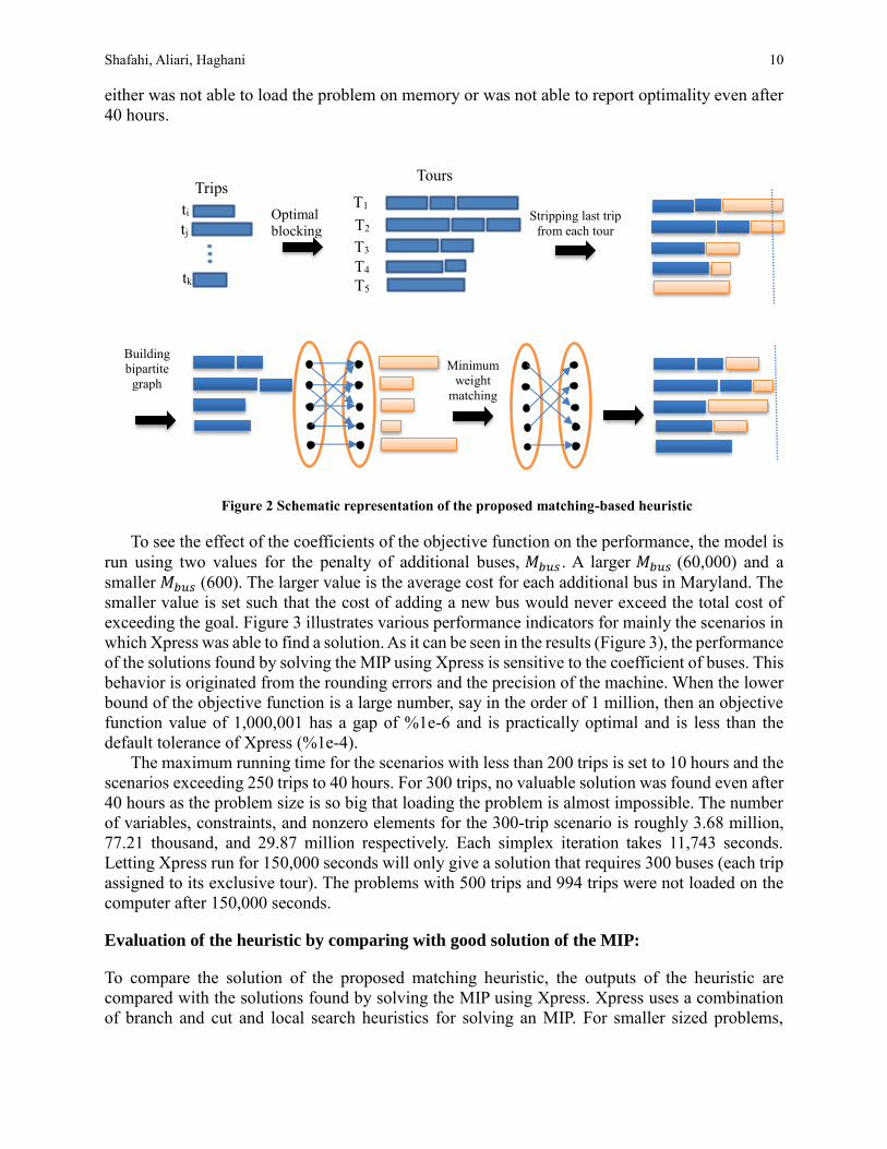
steps of this heuristic are described below, and a summary of the steps is depicted in Figure 2.

• Stage 1: Optimal blocking: Relax the time balancing constraint and obtain an optimal

schedule for the input trips using the assignment-based approach described in (16).

• Stage 2: Balancing modification via perfect matching:

o Step 2-1. Bipartite graph vertex construction: Build the bipartite graph as follows:

Strip the last trip from each tour, and associate a vertex with each stripped tour, and

build set A.

Similarly, associate a vertex with each stripped trip and build set B. Two sets of

vertices of equal size are obtained ready for the bipartite graph.

o Step 2-2. Compatible edge construction: Add an edge between set A, the stripped

tours, and set B, stripped trips, in the bipartite graph, if the linked pair has a

compatible* time window. Afterward, calculate the corresponding weights**.

* Trips a and b are compatible if the end time of current trip (trip a) plus the deadhead to

the next trip (𝐷𝑎𝑏) will not exceed its (trip b) start time.

** The weight for a newly constructed tour is the amount of time the tour operates beyond

the goal (𝑝𝑘𝑛𝑒𝑤).

o Step 2-3. Minimum weight perfect matching: Perform the Hungarian algorithm

(Kuhn–Munkres algorithm) to find the optimal matching.

Granted that the problem is broken into two assignment problems, a drastic decrease in the

computation time is expected.

COMPUTATIONAL RESULTS

In this section, the results of both the mathematical model and the heuristic algorithm are discussed

for 11 different scenarios. All scenarios are built based on two real-world problems. Nine scenarios

are built by sampling from the trips of a real-world case study. For these nine scenarios, a scenario

with 𝑛 trips is built by taking 𝑛 (𝑛 =10,20,30,40,50,100,200,250,300,500) random trips out of the

maximum 994 trips of the real-world data of Howard County Public School System (HCPSS). The

Scenario names are set such that they reflect the number of trips associated with them. The average

duration of the trips is around 25 minutes with the standard deviation of 10 minutes. The minimum

and the maximum duration of the HCPSS trips are 7 and 84 minutes, respectively. A smaller-size

real world problem is also considered for a school district in California that has 54 trips (averages

duration: 40 minutes, minimum duration: 22 minutes, maximum duration: 66 minutes, and the SD:

10 minutes). Given the distribution of the duration for trips and deadheads, it was noticed that a

75-minute goal would illustrate the balancing effects best thus, the goal is set to be equal to 75

minutes in all problems.

The MIP problem is solved by Xpress on a dual processor Intel Xeon computer with a total

192 GB of memory and 40 cores each 2.20GHz. Xpress uses a combination of branch and bound

and heuristic searches at the nodes to search for the optimal solution. Xpress reported the

optimality of the solution for all scenarios with up to 50 trips. However, for larger problems, it


either was not able to load the problem on memory or was not able to report optimality even after

40 hours.

Figure 2 Schematic representation of the proposed matching-based heuristic

To see the effect of the coefficients of the objective function on the performance, the model is

run using two values for the penalty of additional buses, 𝑀𝑏𝑢𝑠 . A larger 𝑀𝑏𝑢𝑠 (60,000) and a

smaller 𝑀𝑏𝑢𝑠 (600). The larger value is the average cost for each additional bus in Maryland. The

smaller value is set such that the cost of adding a new bus would never exceed the total cost of

exceeding the goal. Figure 3 illustrates various performance indicators for mainly the scenarios in

which Xpress was able to find a solution. As it can be seen in the results (Figure 3), the performance

of the solutions found by solving the MIP using Xpress is sensitive to the coefficient of buses. This

behavior is originated from the rounding errors and the precision of the machine. When the lower

bound of the objective function is a large number, say in the order of 1 million, then an objective

function value of 1,000,001 has a gap of %1e-6 and is practically optimal and is less than the

default tolerance of Xpress (%1e-4).

The maximum running time for the scenarios with less than 200 trips is set to 10 hours and the

scenarios exceeding 250 trips to 40 hours. For 300 trips, no valuable solution was found even after

40 hours as the problem size is so big that loading the problem is almost impossible. The number

of variables, constraints, and nonzero elements for the 300-trip scenario is roughly 3.68 million,

77.21 thousand, and 29.87 million respectively. Each simplex iteration takes 11,743 seconds.

Letting Xpress run for 150,000 seconds will only give a solution that requires 300 buses (each trip

assigned to its exclusive tour). The problems with 500 trips and 994 trips were not loaded on the

computer after 150,000 seconds.

Evaluation of the heuristic by comparing with good solution of the MIP:

To compare the solution of the proposed matching heuristic, the outputs of the heuristic are

compared with the solutions found by solving the MIP using Xpress. Xpress uses a combination

of branch and cut and local search heuristics for solving an MIP. For smaller sized problems,

ti

tj

tk

Trips

Tours

T1

T2

T3

T4

T5

Optimal blocking

Stripping last trip

from each tour

Building

bipartite

graph

Minimum

weight

matching


Xpress can find the optimal solution. One important measure and contributor to the overall

transportation cost is the number of buses/tours. The number of buses for the different scenarios

are depicted in Figure 3-a. We can see that for cases in which the problem size is small/medium

(i.e. the number of trips are less than 100), the Xpress solver can find the minimum number of buses.

However, as the problem size exceeds 100 trips, the MIP solver is no longer able to find the

minimum number of buses during its set maximum run-time. For the scenarios with 500 trips or

more in which the MIP solver was not loaded within a 150,000 second time limit, the number of

tours was set equal to the number of trips. Based on these results, it is observable that the MIP

solver loses its value very soon and is only practical for small to medium size scenarios. Thus, it

cannot be used for the HCPSS problem as it will not give any “good” solutions within any

foreseeable time. However, it can find the least number of buses for the small size California

problem.

The second contributor to cost is the excess minutes (Figure 3-b). The transportation authorities

have to pay extra hour fees for those. Comparing the aggregate over time minutes of the heuristic

solutions with the MIP solutions for all scenarios is not fair since in many of the scenarios the

Xpress was not able to find a solution with minimum number of tours within the set time limit. At

the extreme case, if each bus just makes one trip then there will be no excess minutes, but obviously,

the overall cost is a lot more. To make the comparison fair, it is only focused on the scenarios in

which the MIP solver (Xpress) was able to find the minimum number of tours (N10, N20, N30,

N40, N50, N100, N54) or its number of tours was very close to the minimum number (N200). As

it can be seen in Figure3-b, the heuristics solutions are comparable with the solutions from the

MIP solution. A better measure to compare the solutions of the heuristic with those of the MIP

might be the annual cost of each solution that combines the number of buses and the over-hour

costs.

N10 N20 N30 N40 N50 N100 N150 N200 N250 N500 N994 N54

Xpress LargeCoeff 5 9 14 14 19 39 150 73 104 500 994 22

Xpress SmallCoeff 5 9 14 14 19 39 60 85 106 500 994 22

Blocking/Heuristic 5 9 14 14 19 39 56 72 89 163 324 22

0

200

400

600

800

1000

1200

NU

MB

ER O

F B

USE

S (T

OU

RS)

(a) Number of buses comparison for diff Scenarios


Figure 3 (a) Number of buses needed; (b) aggregate minutes exceeding the 75-minute goal; (c) annual

transportation costs; and (d) The net annual benefit/cost of using the heuristic compared with the best solution

found by solving the MIP using Xpress for different scenarios.

Assuming an extra-hour rate of $50/hr and 180 school days per year, the cost for each

additional minute per year is $150. Also, assuming $60,000, the overall cost of the solutions gained

from the heuristic and MIPs as well as the best lower bound found by Xpress are summarized in

N10 N20 N30 N40 N50 N100 N200 N250 N54

Xpress LargeCoeff 0 0 0 198.6961 146.77 175.29 666.1318 797.14 780

Xpress SmallCoeff 0 0 12.68 187.91 119.12 152.3 389.3 723.83 777

Blocking/Heuristic 0.00 0.00 49.60 188.02 165.77 211.32 506.04 947.22 777.00

0

200

400

600

800

1000A

GG

R. D

UR

ATI

ON

EX

CEE

DIN

G

75

MIN

GO

AL

(b) Agg. Duration Exceeding minutes for diff. Scenarios

N10 N20 N30 N40 N50 N100 N200 N250 N54

Xpress LargeCoeff $300,000 $540,000 $840,000 $869,804 $1,162,016 $2,366,294 $4,479,920 $6,359,571 $1,437,000

Xpress SmallCoeff $300,000 $540,000 $841,902 $868,187 $1,157,868 $2,362,845 $5,158,395 $6,468,575 $1,436,550

Blocking/Heurisitc $300,000 $540,000 $847,440 $868,203 $1,164,866 $2,371,698 $4,395,906 $5,482,083 $1,436,550

Best Lower Bound $300,000 $540,000 $841,902 $868,187 $1,152,329 $2,350,086 $4,355,233 $5,437,484 $1,436,550

$0

$1,000,000

$2,000,000

$3,000,000

$4,000,000

$5,000,000

$6,000,000

$7,000,000

TOTA

L TR

AN

SPO

RTA

TIO

N C

OST

($

)

(c) Transportation Cost for diff. Scenarios

N10 N20 N30 N40 N50 N100 N200 N250 N54

Net vs Best $- $- $(7,440 $17 $(6,998 $(8,853 $84,014 $877,48 $-

$(200,000)

$-

$200,000

$400,000

$600,000

$800,000

$1,000,000

AN

NU

AL

NET

BEN

EFIT

FR

OM

USI

NG

H

EUR

ISTI

C O

VER

MIP

($)

(d) Annual Net Benefit / Loss (Comparing with the best result from MIP)


Figure 3-c. Comparison of the best lower bounds of the MIP found by Xpress and the heuristic

solutions indicates a maximum gap of 1.1% and an average gap of 0.5% which accentuates the

effectiveness of the proposed heuristic. The net annual benefit/cost of using the heuristic over the

best result from the MIP is depicted in Figure 3-d. As it can be seen, for those scenarios which are

small enough that the MIP solver can find a good solution, the additional annual cost of the

heuristic’s solution is always less than $10,000. In the California example (N54), the heuristic

finds the optimal solution. However, as the problem size increases, the savings from the heuristic

increase. The heuristic can find a solution that has about 16% less cost for the scenario with 250

trips. For larger scenarios, the MIP solver cannot find any reasonable solution at all even when it

is given a 150,000 second time limit.


Another measure that shows how well the heuristic performs is the number of tours exceeding

the goal. This measurement is interesting as over-hour costs have to be paid for each of the tours

exceeding the goal. If there is a fixed cost component to over hour-costs (such as having a one-

hour minimum duration for over-hours), this measurement turns into a significant one. For

example, if two trips exceed the goal by 5 minutes, the transportation district might need to

purchase an additional hour for each of the buses due to contractual obligations. While this

measurement is not optimized, it is still exciting to see that the heuristic performs okay on this

measurement. As illustrated in Figure 4, the heuristic’ performance is close to the MIP solutions in

all scenarios except for scenario N250 for a 75 minute goal.

Figure 4 Comparison of different methods regarding number of tours exceeding the goal

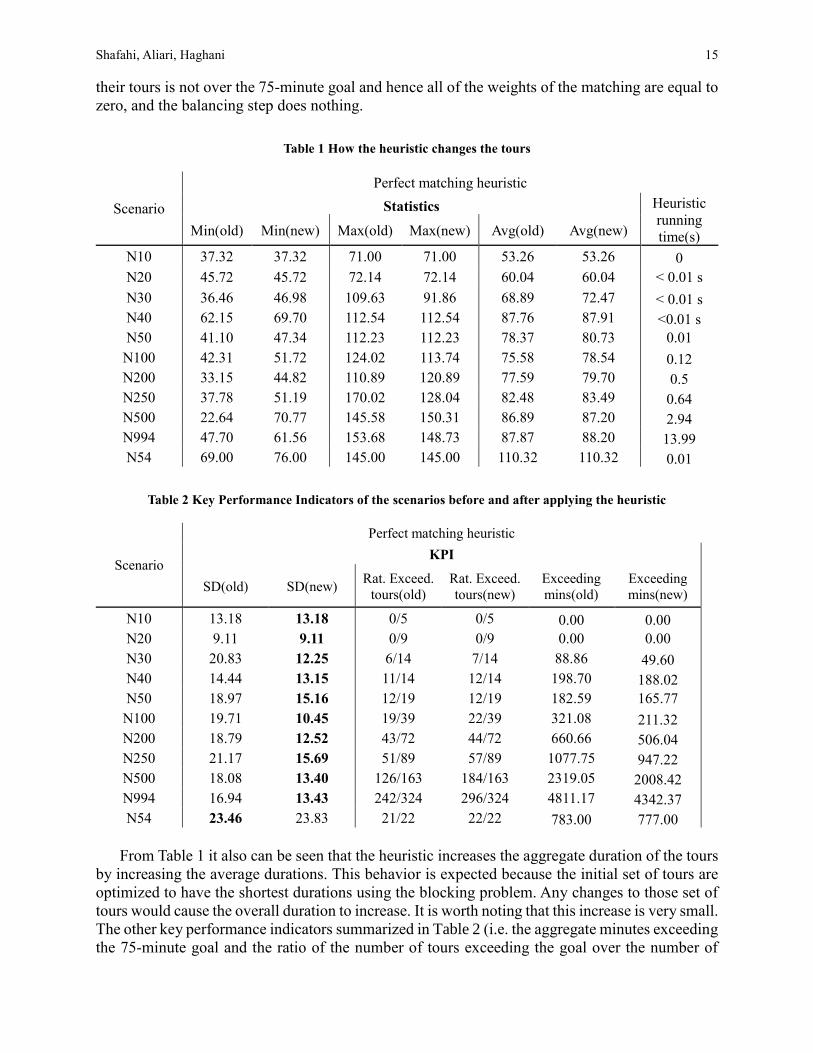
How the heuristic affects the schedule’s key performance indicators (KPI):

The number of buses is a critical KPI. Due to the optimality of the solution during the blocking

stage, it is known that the heuristic provides the minimum number of buses. To illustrate the effect

of the balancing step, the optimal solutions of the blocking problem are compared with the new

solution from the matching heuristic. Recall that the optimal solutions to the blocking problem

primarily minimize the number of tours (buses) and secondarily minimize the aggregate deadhead

time. The heuristic’s performance can be measured based on statistics regarding the tour durations

before and after applying the second stage (balancing-stage). In particular, the focus is on three

KPIs: a) standard deviation of the tours (SD); b) aggregate minutes exceeding the set goal, and c)

percentage of tours exceeding the set goal before (old) and after (new) the balancing stage. Also,

three statistics about the tours are reported, namely, their average, minimum tour duration, and

maximum tour duration. These results are summarized in Table 1 and Table 2. Table 1 shows that

the heuristic acts by increasing the minimum tour duration and usually decreasing the maximum

tour duration. This result is making the tours more balanced as it can be seen in Table 2. The only

case in which the standard deviation increases after applying the heuristic is the California case

study (N54). This increase is only a marginal increase. Therefore, it is observable that the

heuristic’s performance is very satisfactory regarding making more balanced tours. The first two

scenarios with 10 and 20 trips remain unchanged after the balancing step because the duration of

N10 N20 N30 N40 N50 N100 N200 N250

Xpress LargeCoeff 0 0 0 11 10 26 43 45

Xpress SmallCoeff 0 0 5 11 14 25 32 40

Blocking/Heurisitc 0 0 7 12 12 22 44 57

0

10

20

30

40

50

60

# O

F TO

UR

S EX

CEE

DIN

G 7

5 M

IN G

OA

L

Number of Tours Exceeding the 75 min Goal for Different Scenarios


their tours is not over the 75-minute goal and hence all of the weights of the matching are equal to

zero, and the balancing step does nothing.

Table 1 How the heuristic changes the tours

Scenario

Perfect matching heuristic

Statistics Heuristic

running

time(s) Min(old) Min(new) Max(old) Max(new) Avg(old) Avg(new)

N10 37.32 37.32 71.00 71.00 53.26 53.26 0

N20 45.72 45.72 72.14 72.14 60.04 60.04 < 0.01 s

N30 36.46 46.98 109.63 91.86 68.89 72.47 < 0.01 s

N40 62.15 69.70 112.54 112.54 87.76 87.91 <0.01 s

N50 41.10 47.34 112.23 112.23 78.37 80.73 0.01

N100 42.31 51.72 124.02 113.74 75.58 78.54 0.12

N200 33.15 44.82 110.89 120.89 77.59 79.70 0.5

N250 37.78 51.19 170.02 128.04 82.48 83.49 0.64

N500 22.64 70.77 145.58 150.31 86.89 87.20 2.94

N994 47.70 61.56 153.68 148.73 87.87 88.20 13.99

N54 69.00 76.00 145.00 145.00 110.32 110.32 0.01

Table 2 Key Performance Indicators of the scenarios before and after applying the heuristic

Scenario

Perfect matching heuristic

KPI

SD(old) SD(new) Rat. Exceed.

tours(old)

Rat. Exceed.

tours(new)

Exceeding

mins(old)

Exceeding

mins(new)

N10 13.18 13.18 0/5 0/5 0.00 0.00

N20 9.11 9.11 0/9 0/9 0.00 0.00

N30 20.83 12.25 6/14 7/14 88.86 49.60

N40 14.44 13.15 11/14 12/14 198.70 188.02

N50 18.97 15.16 12/19 12/19 182.59 165.77

N100 19.71 10.45 19/39 22/39 321.08 211.32

N200 18.79 12.52 43/72 44/72 660.66 506.04

N250 21.17 15.69 51/89 57/89 1077.75 947.22

N500 18.08 13.40 126/163 184/163 2319.05 2008.42

N994 16.94 13.43 242/324 296/324 4811.17 4342.37

N54 23.46 23.83 21/22 22/22 783.00 777.00

From Table 1 it also can be seen that the heuristic increases the aggregate duration of the tours

by increasing the average durations. This behavior is expected because the initial set of tours are

optimized to have the shortest durations using the blocking problem. Any changes to those set of

tours would cause the overall duration to increase. It is worth noting that this increase is very small.

The other key performance indicators summarized in Table 2 (i.e. the aggregate minutes exceeding

the 75-minute goal and the ratio of the number of tours exceeding the goal over the number of


tours) also show that the heuristic performs well. The heuristic only negatively affects the

percentage of the tours exceeding goal KPI in a meaningful way. However, by making

modifications to the weight calculation procedure in step 2-2 of the algorithm, we can improve

this KPI at the cost of worsening some other. Overall the algorithm does well in balancing as it

reduces the standard deviation by up to 47%. It also reduces the minutes exceeding the goal by up

to 44%.

CONCLUSION

In this paper, a Mixed Integer Model (MIP) formulation of the optimal balanced bus

scheduling/blocking problem is proposed. Solving this formulation yields a balanced schedule

which corresponds to the optimum fleet size. Due to the complexity of the problem, for larger

instances, a matching based heuristic algorithm is proposed. The proposed method can obtain

leading solutions in significantly shorter time for any size problem. However, using the Xpress

MIP solver for solving the proposed MIP is recommended whenever the problem size is tiny so

that the solver can find the optimal solution.

To illustrate the performance of the balancing step of the heuristic, it is depicted that how the

heuristic effects some statistics and key performance indicators of the tours such as the standard

deviation of the tours (SD) and aggregate minutes exceeding the set goal. Statistic measures of the

11 test cases show that the balancing step of the heuristic (the matching phase) always decreases

the aggregate minutes exceeding the goal. In fact, it reduces those by up to 44% in some scenarios.

It is also indicated that in all scenarios related to HCPSS, the standard deviation of the tours

decreases. This reduction in the standard deviation is up to an astonishing 47%.

This study opens the door to research related to balancing of school bus tours. Some possible

future research directions could be: performing the balancing using more general methods such as

min-cost flow; considering more specific versions of the balanced school bus scheduling problem

such as heterogeneous fleet, mixed load, and multiple depots; and incorporation of uncertainties

in balanced scheduling.


REFERENCES

1. Fu, Z., Eglese, R., & Li, L. Y. (2005). A new tabu search heuristic for the open vehicle routing

problem. Journal of the operational Research Society, 56(3), 267-274.

2. Li, F., Golden, B., & Wasil, E. (2007). The open vehicle routing problem: Algorithms, large-scale test

problems, and computational results. Computers & operations research, 34(10), 2918-2930.

3. Orloff, C. S. (1976). Route constrained fleet scheduling. Transportation Science, 10(2), 149-168.

4. Gavish, B., & Shlifer, E. (1979). An approach for solving a class of transportation scheduling

problems. European Journal of Operational Research, 3(2), 122-134.

5. Haghani, A., & Banihashemi, M. (2002). Heuristic approaches for solving large-scale bus transit

vehicle scheduling problem with route time constraints. Transportation Research Part A: Policy and

Practice, 36(4), 309-333.

6. Desaulniers, G., Lavigne, J., & Soumis, F. (1998). Multi-depot vehicle scheduling problems with time

windows and waiting costs. European Journal of Operational Research, 111(3), 479-494.

7. Kliewer, N., Amberg, B., & Amberg, B. (2012). Multiple depot vehicle and crew scheduling with time

windows for scheduled trips. Public Transport, 3(3), 213-244.

8. Kliewer, N., Mellouli, T., & Suhl, L. (2006). A time–space network based exact optimization model

for multi-depot bus scheduling. European journal of operational research, 175(3), 1616-1627.

9. Ceder, A. A. (2011). Public-transport vehicle scheduling with multi vehicle type. Transportation

Research Part C: Emerging Technologies, 19(3), 485-497.

10. Bowerman, R., Hall, B., & Calamai, P. (1995). A multi-objective optimization approach to urban school

bus routing: Formulation and solution method. Transportation Research Part A: Policy and

Practice, 29(2), 107-123.

11. Ripplinger, D. (2005). Rural school vehicle routing problem. Transportation Research Record: Journal

of the Transportation Research Board, (1922), 105-110.

12. Kamali, B., Mason, S. J., & Pohl, E. A. (2013). An analysis of special needs student busing. Journal of

Public Transportation, 16(1), 2.

13. Pacheco, J., Alvarez, A., Casado, S., & González-Velarde, J. L. (2009). A tabu search approach to an

urban transport problem in northern Spain. Computers & Operations Research, 36(3), 967-979.

14. Desrosiers, J., Sauvé, M., & Soumis, F. (1988). Lagrangian relaxation methods for solving the

minimum fleet size multiple traveling salesman problem with time windows. Management

Science, 34(8), 1005-1022.

15. Corberán, A., Fernández, E., Laguna, M., & Marti, R. A. F. A. E. L. (2002). Heuristic solutions to the

problem of routing school buses with multiple objectives. Journal of the operational research

society, 53(4), 427-435.

16. Kim, B. I., Kim, S., & Park, J. (2012). A school bus scheduling problem. European Journal of

Operational Research, 218(2), 577-585.

17. Li, L. Y. O., & Fu, Z. (2002). The school bus routing problem: a case study. Journal of the Operational

Research Society, 552-558.

18. Forbes, M., Holt, J., Kilby, P., & Watts, A. (1991). A matching algorithm with application to bus

operations. Australian Journal of Combinatorics, 4, 71-85.

19. Wark, P., & Holt, J. (1994). A repeated matching heuristic for the vehicle routeing problem. Journal of

the Operational Research Society, 1156-1167.

20. Harvey, N. J., Ladner, R. E., Lovász, L., & Tamir, T. (2006). Semi-matchings for bipartite graphs and

load balancing. Journal of Algorithms, 59(1), 53-78.


21. Shafahi, A., Wang, Z. and Haghani, A., 2017. Solving the school bus routing problem by maximizing

trip compatibility. Transportation Research Record: Journal of the Transportation Research Board,

(2667), pp.17-27. DOI: 10.3141/2667-03.

Documents

BALANCED SCHEDULING OF SCHOOL BUS TRIPS USING A …