Back to the Roots: Solving Polynomial Systems with .../Menu/general/column... · Introduction History Linear Algebra Multivariate Polynomials Applications Conclusions Back to the

Introduction History Linear Algebra Multivariate Polynomials Applications Conclusions

Back to the Roots: Solving Polynomial Systemswith Numerical Linear Algebra Tools

Bart De Moor

Katholieke Universiteit LeuvenDepartment of Electrical Engineering ESAT/SCD

1 / 56


Outline

1 Introduction

2 History

3 Linear Algebra

4 Multivariate Polynomials

5 Applications

6 Conclusions

2 / 56


Why Linear Algebra?

System Identification: PEM

LTI models

Non-convex optimization

Considered ’solved’ early nineties

Linear Algebra approach

⇒ Subspace methods

3 / 56


Why Linear Algebra?

Nonlinear regression, modelling and clustering

Most regression, modelling and clusteringproblems are nonlinear when formulated in theinput data space

This requires nonlinear nonconvex optimizationalgorithms

Linear Algebra approach

⇒ Least Squares Support Vector Machines

‘Kernel trick’ = projection of input data to ahigh-dimensional feature space

Regression, modelling, clustering problembecomes a large scale linear algebra problem (setof linear equations, eigenvalue problem)

4 / 56


Why Linear Algebra?

Nonlinear Polynomial Optimization

Polynomial object function + polynomial constraints

Non-convex

Computer Algebra, Homotopy methods, NumericalOptimization

Considered ’solved’ by mathematics community

Linear Algebra Approach

⇒ Linear Polynomial Algebra

5 / 56


Research on Three Levels

Conceptual/Geometric Level

Polynomial system solving is an eigenvalue problem!Row and Column Spaces: Ideal/Variety ↔ Row space/Kernel of M ,ranks and dimensions, nullspaces and orthogonalityGeometrical: intersection of subspaces, angles between subspaces,Grassmann’s theorem,. . .

Numerical Linear Algebra Level

Eigenvalue decompositions, SVDs,. . .Solving systems of equations (consistency, nb sols)QR decomposition and Gram-Schmidt algorithm

Numerical Algorithms Level

Modified Gram-Schmidt (numerical stability), GS ‘from back to front’Exploiting sparsity and Toeplitz structure (computational complexityO(n2) vs O(n3)), FFT-like computations and convolutions,. . .Power method to find smallest eigenvalue (= minimizer of polynomialoptimization problem)

6 / 56


Four instances of polynomial rooting problems

p(λ) = det(A − λI) = 0(x − 1)(x − 3)(x − 2) = 0

−(x − 2)(x − 3) = 0

x2 + 3y2 − 15 = 0

y − 3x3 − 2x2 + 13x − 2 = 0

minx,y

x2 + y2

s. t. y − x2 + 2x − 1 = 0

7 / 56


Outline

1 Introduction

2 History

3 Linear Algebra


5 Applications

6 Conclusions

8 / 56


Solving Polynomial Systems: a long and rich history. . .

Diophantus(c200-c284)Arithmetica

Al-Khwarizmi(c780-c850)

Zhu Shijie (c1260-c1320) JadeMirror of the Four Unknowns

Pierre de Fermat(c1601-1665)

Rene Descartes(1596-1650)

Isaac Newton(1643-1727)

GottfriedWilhelm Leibniz

(1646-1716)

9 / 56


. . . leading to “Algebraic Geometry”

Etienne Bezout(1730-1783)

Jean-VictorPoncelet

(1788-1867)

August FerdinandMobius (1790-1868)

Evariste Galois(1811-1832)

Arthur Cayley(1821-1895)

Leopold Kronecker(1823-1891)

Edmond Laguerre(1834-1886)

James JosephSylvester

(1814-1897)

Francis SowerbyMacaulay

(1862-1937)

David Hilbert(1862-1943)

10 / 56


So Far: Emphasis on Symbolic Methods

Computational Algebraic Geometry

Emphasis on symbolic manipulations

Computer algebra

Huge body of literature in Algebraic Geometry

Computational tools: Grobner Bases (next slide)

Wolfgang Grobner(1899-1980)

Bruno Buchberger

11 / 56


So Far: Emphasis on Symbolic Methods

Example: Grobner basis

Input system:

x2y + 4xy − 5y + 3 = 0

x2 + 4xy + 8y − 4x − 10 = 0

Generates simpler but equivalent system (same roots)

Symbolic eliminations and reductions

Monomial ordering (e.g., lexicographic)

Exponential complexity

Numerical issues! Coefficients become very large

Grobner Basis:

−9 − 126y + 647y2 − 624y3 + 144y4 = 0

−1005 + 6109y − 6432y2 + 1584y3 + 228x = 0

12 / 56


Outline

1 Introduction

2 History

3 Linear Algebra


5 Applications

6 Conclusions

13 / 56


Homogeneous Linear Equations

Ap×q

Xq×(q−r)

= 0p×(q−r)

C(AT ) ⊥ C(X)rank(A) = r

dim N(A) = q − r = rank(X)

A =[

U1 U2

] [S1 00 0

] [V T

1

V T2

]⇓

X = V2

James Joseph Sylvester

14 / 56


Homogeneous Linear Equations

Ap×q

Xq×(q−r)

= 0p×(q−r)

Reorder columns of A and partition

p×q

A =[p×(q−r) p×r

A1 A2

]rank(A2) = r (A2 full column rank)

Reorder rows of X and partition accordingly

[A1 A2

] [ q−r

X1

X2

]q−r

r

= 0

rank(A2) = r

mrank(X1) = q − r

15 / 56


Dependent and Independent Variables

[A1 A2

] [ q−r

X1

X2

]q−r

r

= 0

X1: independent variables

X2: dependent variables

X2 = −A2† A1 X1

A1 = −A2 X2 X1−1

Number of different ways of choosing r linearly independentcolumns out of q columns (upper bound):(

q

q − r

)=

q!(q − r)! r!

16 / 56


Grassmann’s Dimension Theorem

Ap×q

Xq×(q−rA)

= 0p×(q−rA)

andBp×t

Yt×(t−rB)

= 0p×(t−rB)

What is the nullspace of [A B ]?

[A B ][q−rA t−rB ?

X 0 ?0 Y ?

]= 0

Let rank([A B ]) = rAB

(q − rA) + (t− rB)+? = (p + t)− rAB ⇒ ? = rA + rB − rAB

17 / 56


Grassmann’s Dimension Theorem

[A B ][ q−rA t−rB rA+rB−rAB

X 0 Z1

0 Y Z2

]= 0

Intersection between column space of A and B:

AZ1 = −BZ2

BA

rAB

rA

rA + rB − rAB

rB

#A #B#(A ∪B)

Hermann Grassmann

#(A∪B)=#A +#B−#(A∩B)

18 / 56


Univariate Polynomials and Linear Algebra

Characteristic PolynomialThe eigenvalues of A are the roots of

p(λ) = det(A− λI) = 0

Companion MatrixSolving

q(x) = 7x3 − 2x2 − 5x + 1 = 0

leads to 0 1 00 0 1

−1/7 5/7 2/7

1xx2

= x

1xx2

19 / 56


Univariate Polynomials and Linear Algebra

Consider the univariate equation

x3 + a1x2 + a2x + a3 = 0,

having three distinct roots x1, x2 and x3

24 a3 a2 a1 1 0 00 a3 a2 a1 1 00 0 a3 a2 a1 1

3526666664

1 1 1x1 x2 x3

x21 x2

2 x23

x31 x3

2 x33

x41 x4

2 x43

x51 x5

2 x53

37777775 = 0

Homogeneouslinear system

RectangularVandermonde

corank = 3Observabilitymatrix-like

Realizationtheory!

20 / 56


Two Univariate Polynomials

Consider

x3 + a1x2 + a2x + a3 = 0

x2 + b1x + b2 = 0

Build the Sylvester Matrix:

266641 a1 a2 a3 00 1 a1 a2 a31 b1 b2 0 00 1 b1 b2 00 0 1 b1 b2

37775266664

1x

x2

x3

x4

377775 = 0

Row Space Null SpaceIdeal=union of ideals=multiply rows with pow-ers of x

Variety=intersection of nullspaces

Corank of Sylvester matrix = number of common zeros

null space = intersection of null spaces of two Sylvestermatrices

common roots follow from realization theory in null space

notice ‘double’ Toeplitz-structure of Sylvester matrix

21 / 56



Sylvester ResultantConsider two polynomials f(x) and g(x):

f(x) = x3 − 6x2 + 11x− 6 = (x− 1)(x− 2)(x− 3)

g(x) = −x2 + 5x− 6 = −(x− 2)(x− 3)

Common roots iff S(f, g) = 0

S(f, g) = det

−6 11 −6 1 0

0 −6 11 −6 1−6 5 −1 0 0

0 −6 5 −1 00 0 −6 5 −1

James Joseph Sylvester

22 / 56



The corank of the Sylvester matrix is 2!

Sylvester’s construction can be understood from

1 x x2 x3 x4

f(x) = 0 −6 11 −6 1 0x · f(x) = 0 −6 11 −6 1g(x) = 0 −6 5 −1x · g(x) = 0 −6 5 −1x2 · g(x) = 0 −6 5 −1

1 1x1 x2

x21 x2

2

x31 x3

2

x41 x4

2

= 0

where x1 = 2 and x2 = 3 are the common roots of f and g

23 / 56



The vectors in the canonical kernel K obey a ‘shift structure’:1xx2

x3

x =

xx2

x3

x4

The canonical kernel K is not available directly, instead wecompute Z, for which ZV = K. We now have

S1KD = S2K

S1ZV D = S2ZV

leading to the generalized eigenvalue problem

(S2Z)V = (S1Z)V D

24 / 56


Outline

1 Introduction

2 History

3 Linear Algebra


5 Applications

6 Conclusions

25 / 56


Null space based Root-finding

Considerp(x, y) = x2 + 3y2 − 15 = 0q(x, y) = y − 3x3 − 2x2 + 13x − 2 = 0

Fix a monomial order, e.g., 1 < x < y < x2 < xy <y2 < x3 < x2y < . . .

Construct M : write the system in matrix-vectornotation:

26641 x y x2 xy y2 x3 x2y xy2 y3

p(x, y) −15 1 3q(x, y) −2 13 1 −2 −3x · p(x, y) −15 1 3y · p(x, y) −15 1 3

3775

26 / 56


Null space based Root-finding {p(x, y) = x2 + 3y2 − 15 = 0q(x, y) = y − 3x3 − 2x2 + 13x − 2 = 0

Continue to enlarge M :

it # form 1 x y x2 xy y2 x3 x2y xy2 y3 x4x3yx2y2xy3y4 x5x4yx3y2x2y3xy4y5 →d = 3

p − 15 1 3xp − 15 1 3yp − 15 1 3

q − 2 13 1 − 2 − 3

d = 4

x2p − 15 1 3xyp − 15 1 3y2p − 15 1 3

xq − 2 13 1 − 2 − 3yq − 2 13 1 − 2 − 3

d = 5

x3p − 15 1 3x2yp − 15 1 3xy2p − 15 1 3

y3p − 15 1 3x2q − 2 13 1 − 2 − 3xyq − 2 13 1 − 2 − 3y2q − 2 13 1 − 2 − 3

↓ ...

...

...

...

...

...

...

...

...

...

...

...

...

...

...

...

# rows grows faster than # cols ⇒ overdetermined system

rank deficient by construction!

27 / 56



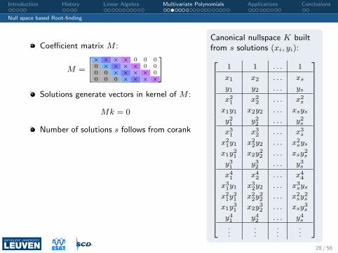
Coefficient matrix M :

M =

"× × × × 0 0 00 × × × × 0 00 0 × × × × 00 0 0 × × × ×

#

Solutions generate vectors in kernel of M :

Mk = 0

Number of solutions s follows from corank

Canonical nullspace K builtfrom s solutions (xi, yi):2666666666666666666666666666664

1 1 . . . 1

x1 x2 . . . xs

y1 y2 . . . ys

x21 x2

2 . . . x2s

x1y1 x2y2 . . . xsys

y21 y2

2 . . . y2s

x31 x3

2 . . . x3s

x21y1 x2

2y2 . . . x2sys

x1y21 x2y2

2 . . . xsy2s

y31 y3

2 . . . y3s

x41 x4

2 . . . x44

x31y1 x3

2y2 . . . x3sys

x21y2

1 x22y2

2 . . . x2sy2

s

x1y31 x2y3

2 . . . xsy3s

y41 y4

2 . . . y4s

......

......

377777777777777777777777777777528 / 56



Choose s linear independent rows in K

S1K

This corresponds to finding lineardependent columns in M

1 1 . . . 1

x1 x2 . . . xs

y1 y2 . . . ys

x21 x2

2 . . . x2s

x1y1 x2y2 . . . xsys

y21 y2

2 . . . y2s

x31 x3

2 . . . x3s

x21y1 x2

2y2 . . . x2sys

x1y21 x2y2

2 . . . xsy2s

y31 y3

2 . . . y3s

x41 x4

2 . . . x44

x31y1 x3

2y2 . . . x3sys

x21y2

1 x22y2

2 . . . x2sy2

s

x1y31 x2y3

2 . . . xsy3s

y41 y4

2 . . . y4s

......

......

29 / 56



Shift property in monomial basis[1 0 0 0 0 00 1 0 0 0 00 0 1 0 0 0

] 1xyx2

xyy2

x =

[0 1 0 0 0 00 0 0 1 0 00 0 0 0 1 0

] 1xyx2

xyy2

[

1 0 0 0 0 00 1 0 0 0 00 0 1 0 0 0

] 1xyx2

xyy2

y =

[0 0 1 0 0 00 0 0 0 1 00 0 0 0 0 1

] 1xyx2

xyy2

Finding the x-roots: let D = diag(x1, x2, . . . , xs), then

S1KD = S2K,

where S1 and S2 select rows from K wrt. shift property

Reminiscent of Realization Theory

30 / 56



Nullspace of M

Find a basis for the nullspace of M using an SVD:

M =

× × × × 0 0 00 × × × × 0 00 0 × × × × 00 0 0 × × × ×

= [ X Y ][

Σ1 00 0

] [W T

ZT

]Hence,

MZ = 0

We haveS1KD = S2K

However, K is not known, instead a basis Z is computed as

ZV = K

Which leads to(S2Z)V = (S1Z)V D

31 / 56



Algorithm

1 Fix a monomial ordering scheme

2 Construct coefficient matrix M

3 Compute basis for nullspace of M , Z

4 Find s linear independent rows in Z

5 Choose shift function, e.g., x

6 Write down shift relation in monomial basis k for the chosen shiftfunction using row selection matrices S1 and S2

7 The construction of above gives rise to a generalized eigenvalueproblem

(S2Z)V = (S1Z)V D

of which the eigenvalues correspond to the, e.g., x-solutions of thesystem of polynomial equations.

8 Reconstruct canonical kernel K = ZV

32 / 56


Data-driven Root-finding

Data-Driven root-finding

Dual version of Kernel-based root-finding

All operations are done on coefficient matrix M

Find linear dependent columns of M instead of linearindependent rows of K (corank)

Write down eigenvalue problem in terms of partitiong of M

Allows sparse representation of M

Rank-revealing QR instead of SVD

33 / 56



{p(x, y) = x2 + 3y2 − 15 = 0q(x, y) = y − 3x3 − 2x2 + 13x − 2 = 0

Finding linear dependent columns of M

1 x y x2 xy y2 x3 x2y xy2 y3 . . .

p − 15 1 3xp − 15 1 3yp − 15 1 3

q − 2 13 1 − 2 − 3x2p − 15xyp − 15y2p − 15

xq − 2 13 1 − 2yq − 2 13 1 − 2

x3p − 15x2yp − 15xy2p − 15

y3p − 15x2q − 2 13 1xyq − 2 13 1y2q − 2 13 1

.

.

.

...

...

...

...

34 / 56


Data-driven Root-finding {p(x, y) = x2 + 3y2 − 15 = 0q(x, y) = y − 3x3 − 2x2 + 13x − 2 = 0

Writing down the eigenvalue problem in terms of a re-orderedpartitioning of M

all linear dependent columns of M corresponding with monomials ofthe lowest possible degree are grouped in M1

M =

[× × × × 0 0 00 × × × × 0 00 0 × × × × 00 0 0 × × × ×

]= [M1 M2]

[M1 M2][

K1

K2

]= 0

K2 = −M†2 M1 K1

(†: Moore-Penrose pseudoinverse)

35 / 56



{p(x, y) = x2 + 3y2 − 15 = 0q(x, y) = y − 3x3 − 2x2 + 13x − 2 = 0

Writing down the eigenvalue problem in terms of a partitioning of M

K1

x1 0. . .

0 xs

= Sx

[K1

K2

]

K1

x1 0. . .

0 xs

= Sx

[Itcr

−M†2M1

]K1

36 / 56


Complications

There are 3 kinds of roots:

1 Roots in zero

2 Finite nonzero roots

3 Roots at infinity

Applying Grassmann’s Dimension theorem on the Kernel allows towrite the following partitioning

[M1 M2][

X1 0 X2

0 Y1 Y2

]= 0

X1 corresponds with the roots in zero (multiplicities included!)

Y1 corresponds with the roots at infinity (multiplicities included!)

[X2;Y2] corresponds with the finite nonzero roots (multiplicitiesincluded!)

37 / 56


Complications

Roots at infinity: univariate case

0 x2 + x− 2 = 0

transform x→ 1X

⇒ X(1− 2X) = 0

1 affine root x = 2 (X = 12)

1 root at infinity x =∞ (X = 0)

Roots at infinity: multivariate case(x− 2)y = 0

y − 3 = 0

transform x→ XT

, y → YT

⇒

XY − 2Y T = 0Y − 3T = 0

1 affine root (2,3,1) (T = 1)

1 root at infinity (1,0,0) (T = 0)

38 / 56


Multiplicities

General Canonical null space K

Multiplicities of roots → multiplicity structure of kernel K

Partial derivatives

∂j1j2...js ≡ ∂x

j11 x

j22 ... xjs

s≡ 1

j1!j2! . . . js!∂j1+j2+...+js

∂xj11 ∂xj2

2 . . . ∂xjss

needed to describe extra columns of K

Currently investigating technicalities

Possibility of trading in multiplicities for extra equations(Radical Ideal)

39 / 56


Multiplicities

Univariate case

f(x) = (x− 1)3 = 0

triple root in x = 1 : f ′(1) = 0 and f ′′(1) = 0

f[

1 3 −3 −1]

1 0 0x 1 0x2 2x 1x3 3x2 3x

= 0

or

∂0f∂1f∂2f

−1 3 −3 13 −6 3 0

−3 3 0 0

1xx2

x3

= 0

40 / 56


Multiplicities

Multivariate case

Polynomial system in 2 unknowns (x, y) with

1 affine root z1 = (x1, y1) with multiplicity 3:[∂00|z1 ∂10|z1 ∂01|z1 ]

1 root z2 = (x2, y2) at infinity: ∂00|z2

M matrix of degree 4

41 / 56


Multiplicities

Canonical Kernel K

K =

∂00|z1 ∂10|z1 ∂01|z1 ∂00|z2

1 0 0 0x1 1 0 0y1 0 1 0x2

1 2x1 0 0x1y1 y1 x1 0y21 0 2y1 0...

......

...x4

1 4x1 0 0x3

1y1 3x21y1 x3

1 1x2

1y21 2x1y

21 2x2

1y1 0x1y

31 y3

1 3x1y21 0

y41 0 4y3

1 0

42 / 56


Polynomial Optimization

Polynomial Optimization Problems

IfA1b = xb

andA2b = yb

then(A2

1 + A22)b = (x2 + y2)b.

(choose any polynomial objective function as an eigenvalue!)

Polynomial optimization problems with a polynomial objective functionand polynomial constraints can always be written as eigenvalue problemswhere we search for the minimal eigenvalue!

→ ‘Convexification’ of polynomial optimization problems

43 / 56


Outline

1 Introduction

2 History

3 Linear Algebra


5 Applications

6 Conclusions

44 / 56


System Identification: Prediction Error Methods

PEM System identification

Measured data {uk, yk}Nk=1

Model structure

yk = G(q)uk + H(q)ek

Output prediction

yk = H−1(q)G(q)uk + (1−H−1)yk

Model classes: ARX, ARMAX, OE, BJ

A(q)yk = B(q)/F (q)uk+C(q)/D(q)ek

H(q)

G(q)

e

u y

Class Polynomials

ARX A(q), B(q)

ARMAX A(q), B(q),C(q)

OE B(q), F (q)

BJ B(q), C(q),D(q), F (q)

45 / 56


System Identification: Prediction Error Methods

Minimize the prediction errors y − y, where

yk = H−1(q)G(q)uk + (1−H−1)yk,

subject to the model equations

Example

ARMAX identification: G(q) = B(q)/A(q) and H(q) = C(q)/A(q), whereA(q) = 1 + aq−1, B(q) = bq−1, C(q) = 1 + cq−1, N = 5

miny,a,b,c

(y1 − y1)2 + . . . + (y5 − y5)

2

s. t. y5 − cy4 − bu4 − (c− a)y4 = 0,

y4 − cy3 − bu3 − (c− a)y3 = 0,

y3 − cy2 − bu2 − (c− a)y2 = 0,

y2 − cy1 − bu1 − (c− a)y1 = 0,

46 / 56


Structured Total Least Squares

Static Linear Modeling

Rank deficiency

minimization problem:

min˛˛ˆ

∆A ∆b˜˛˛2

F,

s. t. (A + ∆A)v = b + ∆b,

vT

v = 1

Singular Value Decomposition:find (u, σ, v) which minimizes σ2

Let M =ˆ

A b˜

8>><>>:Mv = uσ

MT u = vσ

vT v = 1

uT u = 1

Dynamical Linear Modeling

Rank deficiency

minimization problem:

min˛˛ˆ

∆A ∆b˜˛˛2

F,

s. t. (A + ∆A)v = b + ∆b,

vT

v = 1ˆ∆A ∆b

˜structured

Riemannian SVD:find (u, τ, v) which minimizes τ28>><>>:

Mv = Dvuτ

MT u = Duvτ

vT v = 1

uT Dvu = 1 (= vT Duv)

47 / 56



minv

τ2 = vT MT D−1v Mv

s. t. vT v = 1.

0 0.5 1 1.5 2 2.5 30

0.5

1

1.5

2

2.5

3

theta

phi

STLS Hankel cost function

TLS/SVD soln

STSL/RiSVD/invit steps

STLS/RiSVD/invit soln

STLS/RiSVD/EIG global min

STLS/RiSVD/EIG extrema

method TLS/SVD STLS inv. it. STLS eigv1 .8003 .4922 .8372v2 -.5479 -.7757 .3053v3 .2434 .3948 .4535

τ2 4.8438 3.0518 2.3822global solution? no no yes

48 / 56


Maximum Likelihood Estimation

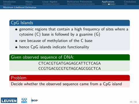
CpG Islands

genomic regions that contain a high frequency of sites where acytosine (C) base is followed by a guanine (G)

rare because of methylation of the C base

hence CpG islands indicate functionality

Given observed sequence of DNA:

CTCACGTGATGAGAGCATTCTCAGA

CCGTGACGCGTGTAGCAGCGGCTCA

Problem

Decide whether the observed sequence came from a CpG island

49 / 56



The model

4-dimensional state space [m] = {A,C,G,T}Mixture model of 3 distributions on [m]

1 : CG rich DNA2 : CG poor DNA3 : CG neutral DNA

Each distribution is characterised by probabilities of observingbase A,C,G or T

Table: Probabilities for each of the distributions (Durbin; Pachter & Sturmfels)

DNA Type A C G T

CG rich 0.15 0.33 0.36 0.16

CG poor 0.27 0.24 0.23 0.26

CG neutral 0.25 0.25 0.25 0.25

50 / 56



The probabilities of observing each of the bases A to T are given by

p(A) = −0.10 θ1 + 0.02 θ2 + 0.25

p(C) = +0.08 θ1 − 0.01 θ2 + 0.25

p(G) = +0.11 θ1 − 0.02 θ2 + 0.25

p(T ) = −0.09 θ1 + 0.01 θ2 + 0.25

θi is probability to sample from distribution i (θ1 + θ2 + θ3 = 1)

Maximum Likelihood Estimate:

(θ1, θ2, θ3) = arg maxθ

l(θ)

where the log-likelihood l(θ) is given by

l(θ) = 11 logp(A) + 14 logp(C) + 15 logp(G) + 10 logp(T )

Need to solve the following polynomial system8<:∂l(θ)∂θ1

=P4

i=1ui

p(i)∂p(i)∂θ1

= 0

∂l(θ)∂θ2

=P4

i=1ui

p(i)∂p(i)∂θ2

= 0

51 / 56



Solving the Polynomial System

corank(M) = 9

Reconstructed Kernel

K =

1 1 1 1 . . .

0.52 3.12 −5.00 10.72 . . .

0.22 3.12 −15.01 71.51 . . .

0.27 9.76 25.02 115.03 . . .

0.11 9.76 75.08 766.98 . . .

......

......

...

1θ1

θ2

θ21

θ1θ2

...

.

θi’s are probabilities: 0 ≤ θi ≤ 1

Could have introduced slack variables to impose this constraint!

Only solution that satisfies this constraint is θ = (0.52, 0.22, 0.26)

52 / 56


And Many More

Applications are found in

Polynomial Optimization Problems


Model order reduction

Analyzing identifiability nonlinear model structures

Robotics: kinematic problems

Computational Biology: conformation of molecules

Algebraic Statistics

Signal Processing

. . .

53 / 56


Outline

1 Introduction

2 History

3 Linear Algebra


5 Applications

6 Conclusions

54 / 56


Conclusions

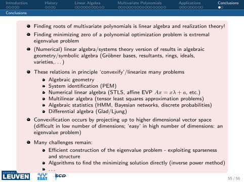
Finding roots of multivariate polynomials is linear algebra and realization theory!

Finding minimizing zero of a polynomial optimization problem is extremaleigenvalue problem

(Numerical) linear algebra/systems theory version of results in algebraicgeometry/symbolic algebra (Grobner bases, resultants, rings, ideals,varieties,. . . )

These relations in principle ‘convexify’/linearize many problems

Algebraic geometrySystem identification (PEM)Numerical linear algebra (STLS, affine EVP Ax = xλ + a, etc.)Multilinear algebra (tensor least squares approximation problems)Algebraic statistics (HMM, Bayesian networks, discrete probabilities)Differential algebra (Glad/Ljung)

Convexification occurs by projecting up to higher dimensional vector space(difficult in low number of dimensions; ‘easy’ in high number of dimensions: aneigenvalue problem)

Many challenges remain:

Efficient construction of the eigenvalue problem - exploiting sparsenessand structureAlgorithms to find the minimizing solution directly (inverse power method). . .

55 / 56


Questions?

Bart De Moor(1960-...)

Kim Batselier(1981-...)

Philippe Dreesen(1982-...)

“At the end of the day,the only thing we really understand,

is linear algebra”.

56 / 56

Documents

Back to the Roots: Solving Polynomial Systems with .../Menu/general/column... · Introduction History Linear Algebra Multivariate Polynomials Applications Conclusions Back to the