Embed Size (px)
Citation preview

PRICAI 2010 Tutorial
P i ll Ob bl M k D i i P Partially Observable Markov Decision Processes Theory and Practice
Pascal Poupart Kee Eung KimPascal Poupart Kee-Eung KimUniversity of Waterloo KAIST

Planning Under Uncertainty P ti ll b bl M k d i i (POMDP ) Partially observable Markov decision processes (POMDPs)
• Naturally model sequential decision making with• Uncertainty in the state of the world• Uncertainty in the state of the world• Uncertainty in action effects• Complex goalsCo ple goals
actiongoals
Agent Environment
goals
Agent Environment
percept
2

Application domains S k di l t Spoken dialogue systems Robotics Resource allocation Resource allocation Preference elicitation Assistive technologiesss st ve tec olog es Health informatics Intelligent tutoring systems Fault recovery systems
3

Tutorial Overview F l d fi iti f POMDP Formal definition of POMDPs
Policies and Value functions
Algorithms for exact and approximate solutionsV l i i• Value iteration
• Policy search• Forward search• Forward search
Case Study 1: COACH (automated planning system for people with dementia)
Case Study 2: Brain-Computer Interface with EEG Case Study 2: Brain Computer Interface with EEG (Electroencephalography)
4

Motivating example S k di l t Spoken dialog system Examples:
• Automated booking/order system• Automated booking/order system• Information retrieval• Call routingCall out g
utterancePerform action
on behalf of user utterance
Spoken dialog system User
on behalf of user
Spoken dialog system User
Speech recognition
5

Formal Model P ti ll Ob bl M k D i i P (POMDP ) Partially Observable Markov Decision Processes (POMDPs)
M = < S,A,O, T, Z,R, b0 >
• : the set of states ( is a state)• : the set of actions ( is an action)S s ∈ SA a ∈ A
• : the set of observations ( is an observation)• : transition probability
b ti b bilit
o ∈ OOT (s, a, s0)
Z( 0 0)
Pr(s0|s, a)P ( 0| 0)• : observation probability
• : immediate reward• : starting probability
Z(a, s0, o0)R(s, a)
b0(s)
Pr(o0|a, s0)
Pr(s)• : starting probability b0(s) Pr(s)
6

Automated lunch box order system St t ibl i t t States: possible user intents
• Quantity: number of lunch boxes• Base: Rice or fried noodles• Base: Rice or fried noodles• Main: eel, squid, salmon, tuna, chicken, pork, or tofu• Veggies: kimchi, sea weed, radish (daicon), bean sprouts, Vegg es: c , sea weed, ad s (da co ), bea sp outs,
spinach, mixed veggies
Actions: system utterances Actions: system utterances• Confirm• Repeatp• Questions
• What kind of veggies would you like?• Do you prefer rice or fried noodles?
7

Automated lunch box order system T iti f ti Transition function
• Stochastic model of how the user intent changes over timetime
• In general: no change• Pr(s’|s,a) = 1 for most state-action pairs
• But user may change intent in some situations
s’Pr(s’|s,a)
Rice“There is no
Rice, eel, kimchi
Rice, tuna, kimchi
Rice salmon kimchi
s a 0.050.3
0.3EelKimchi
There is nomore eel”
Rice, salmon, kimchi
Rice, pork, kimchi
Rice, chicken, kimchi0.150.15
0.05Rice, tofu, kimchi
8

Automated lunch box order system Ob ti tt Observations: user utterances
• In theory: speech signal• In practice: features extracted from speech such as • In practice: features extracted from speech such as
keywords and their negation• Dom(O) = {null,rice,~rice,noodle,~noodle} x
{null,eel,~eel,pork,~pork,…} x {null,kimchi,~kimchi,spinach,~spinach}
Example: “I would like some rice with eel and kimchi”• Speech recognizer may return:
i l ki hi• <rice,eel,kimchi>• <~rice,eel,kimchi>• <rice tuna kimchi>• <rice,tuna,kimchi>• <rice,tuna,null>
9

Automated lunch box order system Ob ti f ti Observation function
• Encodes speech recognition uncertainty and user inconsistenciesinconsistencies
o’Pr(o’|a s’) “I th t
lnull, tuna, nulla s’ 0.75
Pr(o |a,s ) “In that case,I will have some Tuna”
RiceTunaKimchi
“There is nomore eel” null, ~tuna, null
0.2“Is there any Tuna left?”
Kimchi
Null salmon null
0.05 “Ok, I’ll have some salmon then”Null, salmon, null
10

Automated lunch box order system R d f ti i t f Reward function: points for
• Submitting the correct order (100 points)• Taking the order quickly (-1 point per time step)• Taking the order quickly (-1 point per time step)• Keeping the customer happy (-50 points for dropped calls)
Initial belief: distribution over states at the beginning• Distribution corresponding to the likelihood of
lunch box combo
11

Graphical Representation I fl di t ti Influence diagram notation
a0 a1 a2 ah
o0 o1 o2 oh
T T TTZ Z Z Z
s0 s1 s2 sh...T T TT
R R R R
r0 r1 r2 rh+ ...+ + 2 + h
Solution: policy that maximizes expected total rewards12

Graphical Representation POMDP i t i f th HMM POMDP is an extension of the HMM
a0 a1 a2 ah
o0 o1 o2 oh
T T TTZ Z Z Z
s0 s1 s2 sh...T T TT
R R R R
r0 r1 r2 rh+ ...+ + 2 + h
Solution: policy that maximizes expected total rewards13
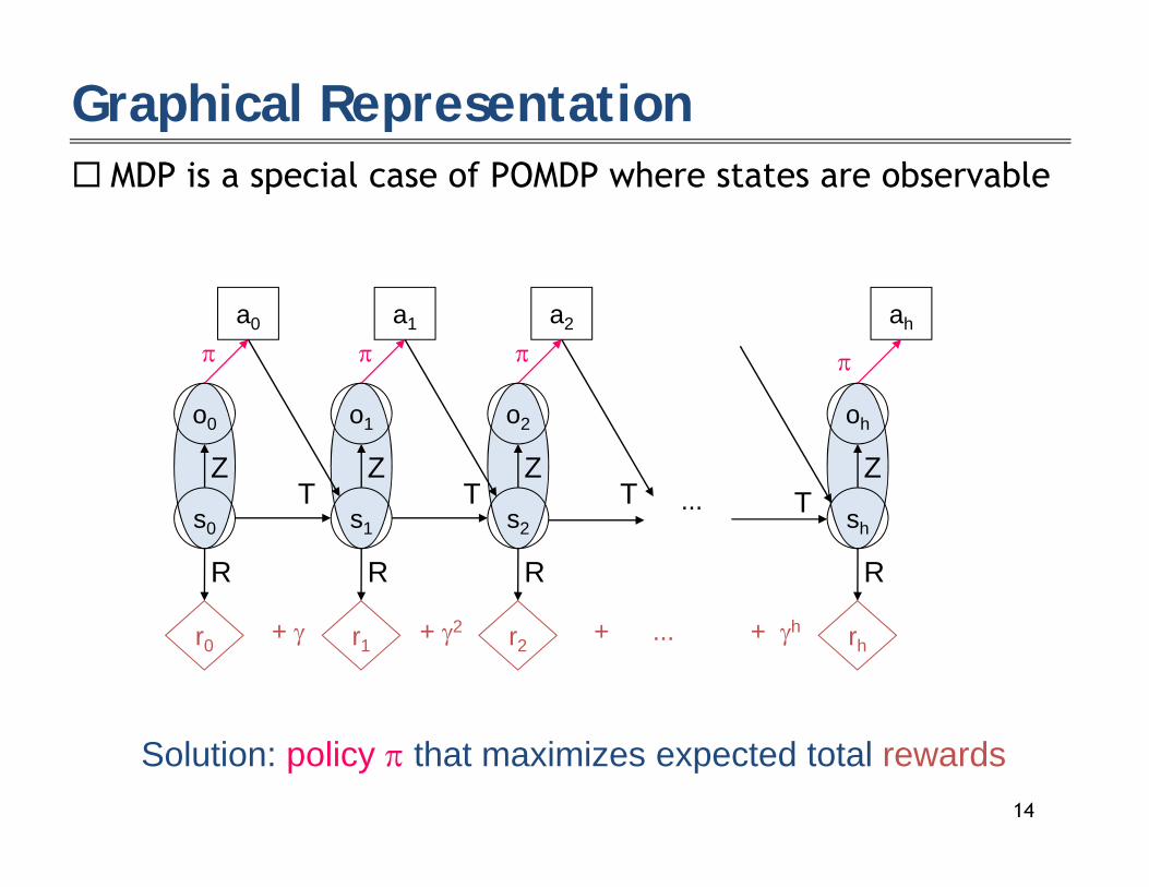
Graphical Representation MDP i i l f POMDP h t t b bl MDP is a special case of POMDP where states are observable
a0 a1 a2 ah
o0 o1 o2 oh
T T TTZ Z Z Z
s0 s1 s2 sh...T T TT
R R R R
r0 r1 r2 rh+ ...+ + 2 + h
Solution: policy that maximizes expected total rewards14

Tutorial Overview F l d fi iti f POMDP Formal definition of POMDPs
Policies and Value functions
Algorithms for exact and approximate solutionsV l i i• Value iteration
• Policy search• Forward search• Forward search
Case Study 1: COACH (automated planning system for people with dementia)
Case Study 2: Brain-Computer Interface with EEG Case Study 2: Brain Computer Interface with EEG (Electroencephalography)
15

Tutorial Overview F l d fi iti f POMDP Formal definition of POMDPs
Policies and Value functions
Algorithms for exact and approximate solutionsV l i i• Value iteration
• Policy search• Forward search• Forward search
Case Study 1: COACH (automated planning system for people with dementia)
Case Study 2: Brain-Computer Interface with EEG Case Study 2: Brain Computer Interface with EEG (Electroencephalography)
16

Policies P li i ( ) i f i iti l b li f d hi t i t Policies (): mapping from initial beliefs and histories to
actions
π : < b0, ht >→ at
Histories (h): past actions and observations
hht ≡ < a0, o1, a1, o2, . . . , at−1, ot >
17

Conditional plan F h i iti l b li f th li i t f diti l For each initial belief, the policy consists of a conditional
plan that can be represented by a treeStages to go
β
a1o1 o2
3
g g
a3 a2
1 2
oooo
2
a1 a2 a1 a3
o2o1o2o1
1
Two problems:• Growing histories• Exponentially large conditional plans
18

Finite state controllers C ll ti f li diti l l Collection of cyclic conditional plans
aa2
o2 o2a1
a1
o1o2o1
o1
a3
1a3 o1
o1
1o1
o2
oa2
o2o2
19

Belief mapping Alt ti li t ti Alternative policy representation:
π : bt → at
Sufficient statistic:
b ≡ < b h > ≡ < b >bt ≡ < b0, ht > ≡ < b0, a0, o1, a1, o2, . . . , ot >),,,,,,|Pr()( 21100 ttt ooaoabsSsb
Incremental update: Bayes Theorem
bao0 ≡ < b, a, o0 >
bao0(s0) = k
Ps b(s) Pr(s
0|s, a) Pr(o0|a, s0)
20

Evaluation V l t f d d ti Value: amount of reward earned over time
Several criteria Several criteria• Total or average reward• Expected or worst case rewardpected o wo st case ewa d• Discounted or undiscounted reward
Most common criterion: total, expected, discounted reward
V π(b0) =Ph
t=0 γtP
s bt(s)R(s, π(bt))
A policy is optimal when
( 0)P
t=0 γP
s t( ) ( , ( t))
∗π∗
V π∗(b) ≥ V π(b) ∀b21

Optimal Value Function S ll d d S dik ti l l f ti i i i Smallwood and Sondik: optimal value function is piece-wise
linear and convex
V
belief spaceb(s1)=0 b(s1)=1
22

Conditional plan value function V l f ti f diti l l β Value function of a conditional plan
• Linear with respect to belief space• Often called an alpha-vector
β
• Often called an alpha-vector
V
α
belief spaceb(s1)=0 b(s1)=1
23

Conditional plan value function R i t ti Recursive construction
• One-step conditional plan: one for each action• = execute action aβ1• = execute action a1β1
V
αβ1
belief spaceb(s1)=0 b(s1)=1
24

Conditional plan value function R i t ti Recursive construction
• One-step conditional plan: one for each action• = execute action aβ1• = execute action a1
• = execute action a2
β1β2
Vαβ2
belief spaceb(s1)=0 b(s1)=1
25

Conditional plan value function R i t ti Recursive construction
• two-step conditional plan: execute an action and then execute an one-step conditional plan branching on observationp p g
• e.g. = execute a1 and then execute regardless of observation
β3 β1
V a1o1 o2
a1 a1
1 2
belief spaceb(s1)=0 b(s1)=1
αβ3(s) = R(s, a1) + γP
s0∈S T (s, a1, s0)Z(a1, s0, o1)αβ1(s0)( ) ( , ) γ
Ps ∈S ( , , ) ( , , ) ( )
+ γP
s0∈S T (s, a1, s0)Z(a1, s0, o2)αβ1(s0)
26
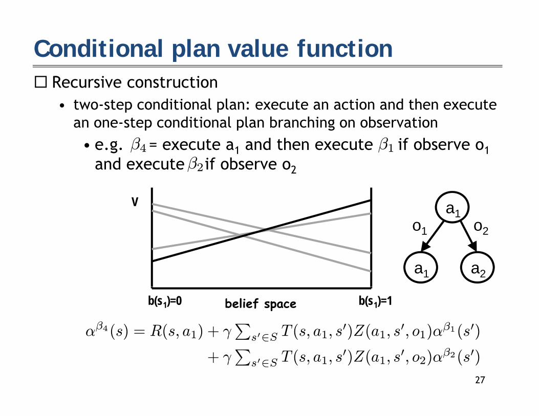
Conditional plan value function R i t ti Recursive construction
• two-step conditional plan: execute an action and then execute an one-step conditional plan branching on observationp p g• e.g. = execute a1 and then execute if observe o1
and execute if observe o2
β4 β1β2
V a1o1 o2
a1 a2
1 2
belief spaceb(s1)=0 b(s1)=1
αβ4(s) = R(s, a1) + γP
s0∈S T (s, a1, s0)Z(a1, s0, o1)αβ1(s0)( ) ( )
Ps ∈S ( ) ( ) ( )
+ γP
s0∈S T (s, a1, s0)Z(a1, s0, o2)αβ2(s0)
27

Conditional plan value function R i t ti Recursive construction
• n-step conditional plan: execute an action and then execute an (n-1)-step conditional plan branching on observation( ) p p g
•a
o o
(n-1) step conditional plans
|Γn| = |A||Γn−1||O|
o1 o2V
plans
β0 β00
αβ(s) = R(s, a) + γP
s0∈S T (s, a, s0)Z(a, s0, o1)αβ0(s0)
belief spaceb(s1)=0 b(s1)=1
+ γP
s0∈S T (s, a, s0)Z(a, s0, o2)αβ00(s0)
28

Optimal Value Function O ti l l f ti V ∗ Optimal value function :
• upper surface of a set of -vectorsV ∗
Γ∗ α
V
belief spaceb(s1)=0 b(s2)=1
Satisfies Bellman’s equation • Satisfies Bellman s equation
29

Tutorial Overview F l d fi iti f POMDP Formal definition of POMDPs
Policies and Value functions
Algorithms for exact and approximate solutionsV l i i• Value iteration
• Policy search• Forward search• Forward search
Case Study 1: COACH (automated planning system for people with dementia)
Case Study 2: Brain-Computer Interface with EEG Case Study 2: Brain Computer Interface with EEG (Electroencephalography)
30

Solution algorithms Offli l ith Offline algorithms
• Value iteration• Policy search• Policy search
Online algorithmsO l e algo t s• Forward search
In practice: combine online and offline techniques• Offline: find approximate policy• Online: refine it
31

Tutorial Overview F l d fi iti f POMDP Formal definition of POMDPs
Policies and Value functions
Algorithms for exact and approximate solutionsV l i i• Value iteration
• Policy search• Forward search• Forward search
Case Study 1: COACH (automated planning system for people with dementia)
Case Study 2: Brain-Computer Interface with EEG Case Study 2: Brain Computer Interface with EEG (Electroencephalography)
32

Value Iteration I t h ll In a nutshell:Initialize Γ1 = {α-vectors for each 1-step conditional plan}for n = 1; value has not converged; n++ doCompute Γn+1 = {α-vectors for each (n+1)-step conditional plan}using Γn = {α-vectors for each n-step conditional plan}(use recursive definition)
Termination condition
( )end for
• Value convergence:where and
Challenge• Creates exponentially many α-vectors: |Γn+1| = |A||Γn||O|• Creates exponentially many α vectors: |Γn+1| |A||Γn|
33

Pruning α-vectors M t f th t t d i h it ti b Most of the α-vectors generated in each iteration may be
redundant• Remove those not participating in the upper surfaceRemove those not participating in the upper surface
V
Pruning by linear programmingbelief spaceb(s1)=0 b(s2)=1
Maximize: δDomination Constraints: for each α0 ∈ Γ\α: α · b− α0 · b ≥ δSimplex Constraints: for each s ∈ S: b(s) ≥ 0 and Ps b(s) = 1
• If δ ≤ 0, α can be removed from S p e Co st a ts o eac s ∈ S b(s) ≥ 0 a d Ps b(s)
34

Point-Based Value Iteration [Pineau et al.]
P i i ti l b t till t t t i Pruning is essential but still generates too many -vectors in practice
PBVI insight: rather than generating -vectors for all possible beliefs in the simplex, focus computation on reachable beliefsbeliefs• Obtain some finite set of belief points B• for each action a A•
for each action a A and observation o O• for each b B and a A• for each b B and a A•
Bounded number of -vectors: |’| = |B|
35

Other Point-based Solvers M tl diff i h th b li f t i t d Mostly differ in how the belief set is generated
• Random, heuristic search
Other point-based solvers• Perseus [Spaan and Vlassis, 2005]e seus [Spaa a d Vlass s, 005]• Heuristic Search Value Iteration (HSVI) [Smith and
Simmons, 2004]• SARSOP [Kurniawati, Hsu and Lee, 2004]• Forward Search Value Iteration (FSVI) [Shani, Brafman,
Shimony 2007]Shimony, 2007]
36

Symbolic Solvers Flat solvers Flat solvers
• Matrices and vectors• Largest problems solved: ~10,000 states
Symbolic solvers• Algebraic decision diagrams (ADDs)• E.g. Symbolic Perseus [Poupart, 05] and Symbolic HSVI [Sim et
al., 08]• Largest problems solved: ~50,000,000 states
naturally exploit structure• aggregate states with identical (or similar values)• Exploit factored structure
• Context independence, context specific independence• Exploit sparsityExploit sparsity
• Mixed observability
37

S b li d l h ki [B h l 93]
Algebraic Decision Diagrams Symbolic model-checking [Bahar et al. 93]
Factored MDPs: SPUDD [Hoey et al. 98] X Y Z Pr(X,Y,Z)
1 1 1 0 05
Example: joint distribution over {X,Y,Z}
1 1 1 0.05
1 1 2 0.05
1 2 1 0.05
X
1 2 2 0.05
2 1 1 0.08
2 1 2 0 08
Equivalent ADD
Y Y0.05
12
32 1 2 0.08
2 2 1 0.2
2 2 2 0.4
0.08 Z 0.021 1
1
2
2
2 3 1 1 0.2
3 1 2 0.4
3 2 1 0.02
0.2 0.4 3 2 2 0.02
38

T d l ti f ith ti ti
Efficient manipulation Top-down evaluation of arithmetic operations
• Size of resulting ADD:W t ti l i b f i bl• Worst case: exponential in number of variables
• Very often: polynomial in number of variablesEvaluation time: linear in size of resulting ADD• Evaluation time: linear in size of resulting ADD
+ A
C
B
9B
A
3 C
B
13C
B
12C
7 8
9B
4 5
3 C
12 13
13C
10 11
12
39

Tutorial Overview F l d fi iti f POMDP Formal definition of POMDPs
Policies and Value functions
Algorithms for exact and approximate solutionsV l i i• Value iteration
• Policy search• Forward search• Forward search
Case Study 1: COACH (automated planning system for people with dementia)
Case Study 2: Brain-Computer Interface with EEG Case Study 2: Brain Computer Interface with EEG (Electroencephalography)
40

Policy Search Pi k li t ti Pick a policy representation
• Common choice: finite state controllers
Ideas: alternate between• Policy improvementol cy p ove e t• Policy evaluation
Algorithms• Policy Iteration [Hansen 97]• Policy search techniques for bounded controllers
41

Policy Iteration [H 97] P li It ti [Hansen 97] Policy Iteration
• Alternate between policy evaluation and policy improvementimprovement
Policy improvement
Policy evaluationCompute V π(b)
42

Finite state controller P t i ti φ Parameterization:
• Action mapping: • Successor node mapping:
σ(n) = a
φ(n o) = n0
π ≡ < σ,φ >
• Successor node mapping:
ao2 o
φ(n, o) = n
a1
a2
o1o2o1
o2 o2
a1a3 o1
o1
o1o1
o2a3
a2
o12
o2o2
43

Policy Evaluation S l li t Solve linear system
V
Belief space
44

C d f ll ibl d
Policy Improvement [Hansen]φ Create new nodes for all possible and
• Total of |A||N||O| new nodes
σ φ
a1
o1
o1
a1a1o2
1 o2
o1
a2
a1o1
o2o2
o1
o2
2
a2o2
o1o2
45

R i l bl d i i d
Policy Improvement [Hansen] Retain only blue dominating nodes
• i.e. those part of the upper surface
a1
o1
o1
a1a1o2
1 o2
o1
a2
a1o1
o2o2
o1
o2
2
a2o2
o1o2
46
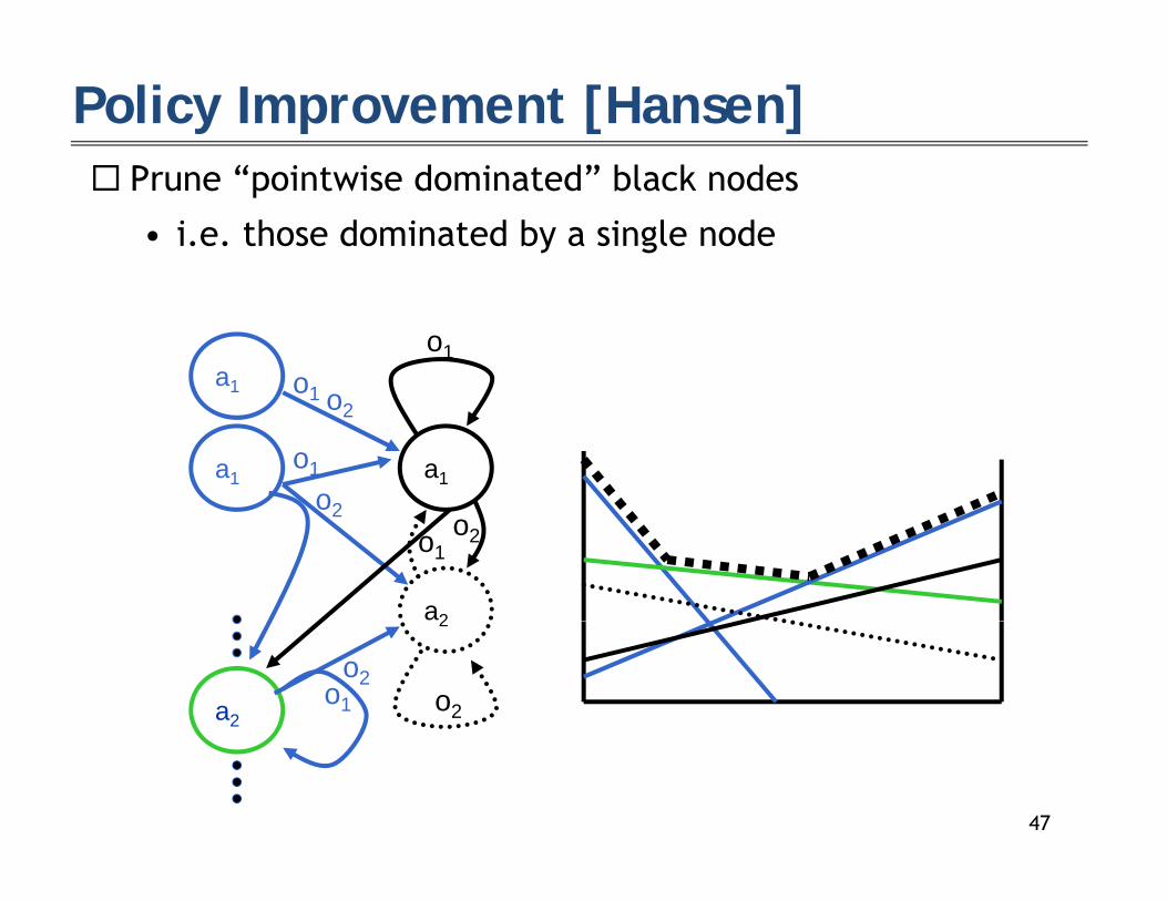
P “ i i d i d” bl k d
Policy Improvement [Hansen] Prune “pointwise dominated” black nodes
• i.e. those dominated by a single node
a1
o1
o1
a1a1o2
1 o2
o1
a2
o1
o2 o2
2
a2o2
o1
o2
47

P bl ll d i ll !
Exponential Growth Problem: controllers tend to grow exponentially!
• At each iteration, up to |A||N||O| nodes may be added
Solution: Bounded Controllers
48

Policy Search for Bounded Controllers
Gradient ascent [Meuleau et al. 99, Aberdeen & Baxter 02] Branch and bound [Meuleau et al. 99] Stochastic Local Search [Braziunas, Boutilier 04] B d d li i i [P 03] Bounded policy iteration [Poupart 03] Non-convex optimization [Amato et al. 07]M i lik lih d [T i t t l 06]Maximum likelihood [Toussaint et al. 06]
49

Stochastic Controllers
Policy search often done with stochastic controllers
( ) P ( | )σ(n) = Pr(a|n)φ(n, o0) = Pr(n0|n, o0)
Why?
• Continuous parameterization
Pr(a)
o
o20.3
• Continuous parameterization
• More expressive policy space
o10.7
0.6
0.4
50

Bounded Policy Improvement
Improve each node in turn [Poupart, Boutilier 03]
R l ith d i ti t h ti d• Replace with dominating stochastic node
51

Bounded Policy Improvement
Improve each node in turn [Poupart, Boutilier 03]
R l ith d i ti t h ti d• Replace with dominating stochastic node
52

Node Improvement
Linear Programming
Objective:
Variables: max ²
{Pr(a, n0|n, o0),Pr(a|n)}
Constraints: αn(s) + ² ≤P
a[Pr(a|n)R(a, s)+γP
s0o0n0 Pr(s0|s, a) Pr(o0|s0, a) Pr(a, n0|n, o0)αn0(s0)]
Pr(a|n) PPr(a n0|n o0) ∀a n o0
O(|S|+|A||O|) constraints
Pr(a|n) =Pn0 Pr(a, n0|n, o0) ∀a, n, o0
O(|S|+|A||O|) constraints
O(|A||O||N|) variables
53

Non-convex optimization
[Amato et al. 07]
Objective:
Variables:max
Ps b0(s)α0(s)
{Pr(a, n0|n, o0),Pr(a|n),αn(s)}
Constraints: αn(s) =P
a[Pr(a|n)R(a, s)+γP
s0o0n0 Pr(s0|s, a) Pr(o0|s0, a) Pr(a, n0|n, o0)αn0(s0)]
Quadratically constrained problem
Pr(a|n) =Pn0 Pr(a, n0|n, o0) ∀a, n, o0
Quadratically constrained problem
|N| more variables and constraints than LPs in BPI
54

Planning as Inference [Toussaint et al.]
Idea: convert POMDP into a planning problem
R l d f ti t b b t 0 d 1• Re-scale reward function to be between 0 and 1
• Treat policy parameters as unknown conditional probability tablesprobability tables
Policy optimization Policy optimization
•
• EM algorithm
maxσ,φ Pr(r|σ,φ)EM algorithm
55

Graphical Model
[Meuleau et al. 99]
I fl di th t i l d t ll Influence diagram that includes controller
’
o o’
n’n
a
s s’
o oa
s s
’r r’
56

Likelihood Maximization
n0• [Toussaint et al. 06] • Mixture of DBNs with
s0
o0
r0
• Mixture of DBNs with normalized terminal reward1-
n1n0
(1 )
s0 s1
o0 o1a0
r1...
(1-)
o1 o2
n2n1
a1o0
n0
a0 ok
nk
a2 ...
...
k(1-)
s1 s2
o1 o2a1
s0
o0 a0
sk
oka2
rk
( )
57

Expectation Maximization
Alternate betweenE t ti• ExpectationsE(n, a) =
Pt γ
t Pr(Nt = n,At = a|σ,φ, r = 1)E(n, o0, n0) =
Pt γ
t Pr(Nt = n,Ot+1 = o0, Nt+1 = n0|σ,φ, r = 1)
• Policy improvement
E(n, o , n )P
t γ Pr(Nt n,Ot+1 o ,Nt+1 n |σ,φ, r 1)
• Policy improvementσ = Pr(n|a) = E(n, a)/Pa E(n, a)φ = Pr(n0|n, o0) = E(n, o0, n0)/Pn0 E(n, o
0, n0)φ ( | ) ( )/P
n ( )
58

Other Policy Search Techniques
Policy search via density estimation [Ng et al. 99] PEGASUS [N J d 00] PEGASUS [Ng, Jordan 00] Gradient-based policy search [Baxter, Bartlett 00] Natural policy gradient [Kakade 02] Natural policy gradient [Kakade 02] Covariant policy search [Bagnell, Schneider 03] Policy search by dynamic programming [Bagnell et al 04] Policy search by dynamic programming [Bagnell et al. 04] Point-based policy iteration [Ji, Parr et al. 07]
59

Tutorial Overview F l d fi iti f POMDP Formal definition of POMDPs
Policies and Value functions
Algorithms for exact and approximate solutionsV l i i• Value iteration
• Policy search• Forward search• Forward search
Case Study 1: COACH (automated planning system for people with dementia)
Case Study 2: Brain-Computer Interface with EEG Case Study 2: Brain Computer Interface with EEG (Electroencephalography)
60

Forward search O li l ith Online algorithm Expectimax forward search
maxa1
a2
expo1 o2
expo1 o2
maxa1 a2
maxa1 a2
maxa1 a2
maxa1 a2
exp exp exp expo1 o2 o1 o2 o1 o2 o1 o2
exp exp exp expo1 o2 o1 o2 o1 o2 o1 o2
V1 V2 V3 V4 V5 V6 V7 V8 V9 V10 V11 V12 V13 V14 V15 V16
61

In practice L f d Leaf nodes:
• Values from some approximate solution computed offline
Max nodes:• Branch and bounda c a d bou d• Prune dominated subtrees
Expectation nodes:• Sample subset of observations• Prune subtrees that are not sampled
62

Tutorial Overview F l d fi iti f POMDP Formal definition of POMDPs
Policies and Value functions
Algorithms for exact and approximate solutionsV l i i• Value iteration
• Policy search• Forward search• Forward search
Case Study 1: COACH (automated planning system for people with dementia)
Case Study 2: Brain-Computer Interface with EEG Case Study 2: Brain Computer Interface with EEG (Electroencephalography)
63

A d i
COACH project Automated prompting system
to help elderly persons wash their hands
Planning done with a POMDP Planning done with a POMDP
64

System Overview
sensors decisionmaking
hand verbalhandwashing
verbal cues
65

Computer Vision (Preprocessing)
Location (x,y coord) of hands and towel• Particle filtering (flock of particles)
66

A ti t A
POMDP Components Action set A
• DoNothing, CallCaregiver, Prompt {turnOnWater, rinseHands useSoap }Hands, useSoap, …}
State set S = dom(HL) x dom(WF) x dom(D) x State set S = dom(HL) x dom(WF) x dom(D) x …• Hand Location {tap,water,soap,towel,sink,away,…}• Water Flow {on off}Water Flow {on, off}, • Dementia {high, low}, etc.
Observation set O = dom(C) x dom(FS)• Camera {handsAtTap, handsAtTowel, …}{ p, , }• Faucet sensor {waterOn, waterOff}
67

State Variables (I)
Environment variables• WaterFlow (WF)• HandLocation (HL) water
Sensor Observations• ObservedWaterFlow (OWF)
Ob dH dL ti (OHL)• ObservedHandLocation (OHL)
Pr(OWF|WF=yes)Pr(OHL|HL=tap)
31%55%
7% 7%
Pr
Pr(OWF|WF yes)
99%Pr
OHL
7% 7%
OWF
1%
68

State Variables (II)
Activity status variables Activity status variables• PlanStep• MaxPlanStep
Task starts
Turn on waterUse soapp• RepeatedPlanStep• Progress
Wet hands
Rinse hands
Use soapTurn on water
g Rinse hands
Dry handsTurn off water
Task over
Turn off waterDry hands
69

State Variables (III)
User specific variablesA { }• Aware {never, no, yes}
• Models need for assistance
• Responsive {none video max min}• Responsive {none, video, max, min}• Models response to assistance
• Dementia level {low med high}Dementia level {low, med, high}• Likelihood user will be aware and responsive
Allow adaptation to user
70

Transition Probabilities
Dynamics: Pr(s’|s,a)• Turn on water
sink,off0.3
0 6sink,off tap,on
soap,off
0.6
0.05
• Probabilities specified by domain expert• Probabilities specified by domain expert
71
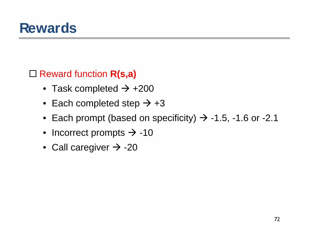
Rewards
Reward function R(s a) Reward function R(s,a)• Task completed +200• Each completed step +3Each completed step +3• Each prompt (based on specificity) -1.5, -1.6 or -2.1• Incorrect prompts -10Incorrect prompts 10• Call caregiver -20
72

Policy Optimization
Symbolic Perseus Packagehtt // t l / t/ ft ht l• http://www.cs.uwaterloo.ca/~ppoupart/software.html
• Point-based value iterationSymbolic representation (algebraic decision diagrams)• Symbolic representation (algebraic decision diagrams)
• Handles large state spaces
COACH POMDP• 207,306 states, 198 observations, 26 actions• Takes about 1 day to optimize policy (single core
computer)
73

Empirical Comparison (Simulation)
74

COACH Video
75

R f
References References
• Boger, Poupart, Hoey, Boutilier, Fernie, and Mihailidis, A Decision-Theoretic Approach to Task Assistance for Persons with Dementia, IJCAI, pages 1293-1299, 2005
• Hoey, Poupart, von Bertoldi, Craig, Boutilier, Mihailidis, oey, oupa t, vo e told , C a g, out l e , M a l d s, Automated Handwashing Assistance for Persons with Dementia using Video and a Partially Observable Markov Decision Process, ov Decision Process, Computer Vision and Image Understanding, 114 (5), 503-519, 2010.
On going project • Alex Mihailidis (University of Toronto)• Jesse Hoey (University of Waterloo)
76

Tutorial Overview F l d fi iti f POMDP Formal definition of POMDPs
Policies and Value functions
Algorithms for exact and approximate solutionsV l i i• Value iteration
• Policy search• Forward search• Forward search
Case Study 1: COACH (automated planning system for people with dementia)
Case Study 2: Brain-Computer Interface with EEG Case Study 2: Brain Computer Interface with EEG (Electroencephalography)
77

Sensing & Interfacing the Brainel
ay
r Tim
e D
eon
und
er
Y.K
. Son
g
al e
xecu
ti
Cou
rtesy
of
(SN
U)
Opt
ima
Optimal execution under Sensory Uncertainty78

Electroencephalogram(EEG) & P300
Electroencephalogram (EEG)A
Target
Non‐target
P300Preprocessor
Feature extraction Spatial filter algorithmA i f EEG i l Averaging of EEG signalsMexican hat wavelet
79

Conventional Stimulus Scheme E h L tt i fl h d i 250 i t l Each Letter is flashed in 250ms intervals
• Turn on for 125ms, turn off for 125ms• Letter flashing sequences are • Letter flashing sequences are
generated uniformly at random
Trial and Test• Trial = a sequence of flashes for every letter• Test = multiple trials for deciding the target letter
TestTest
80

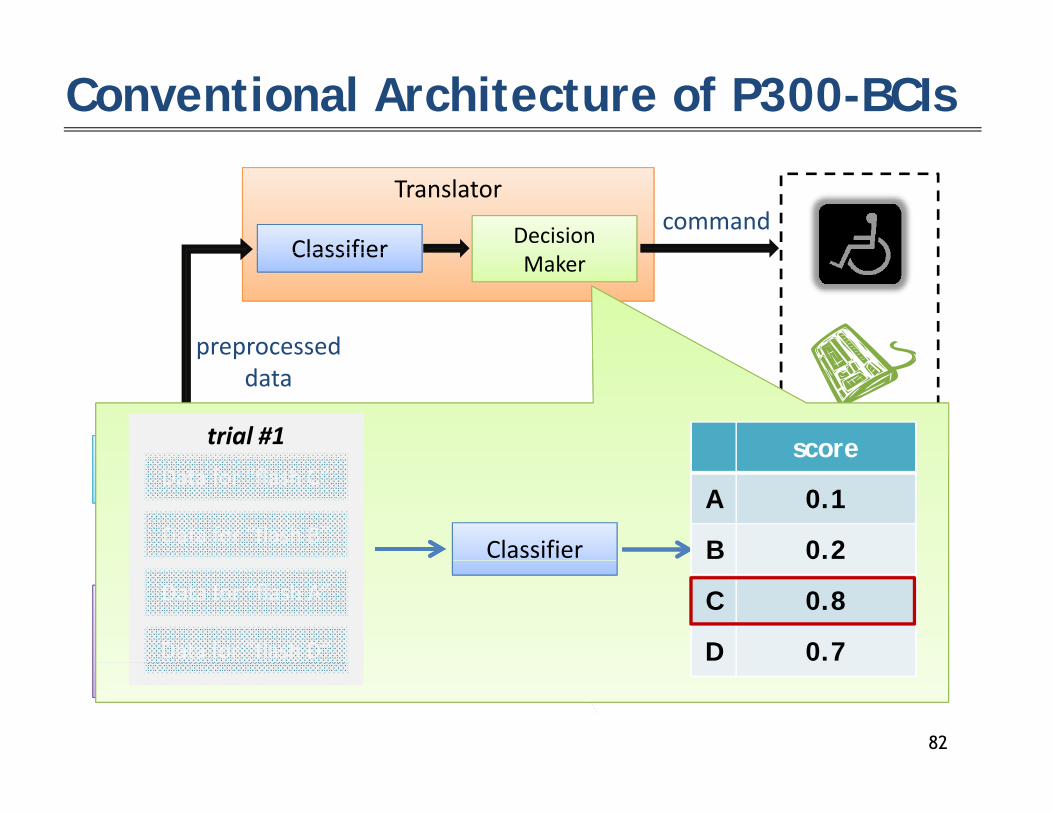
Conventional Architecture of P300-BCIs
Translator
Classifier Decision command
preprocessed
Classifier Maker
R lp pdata Role
classify the input signal for existence of P300 (0‐1 classification)
Training DataPreprocessor
EEG signal
positive instances ‐ preprocessed signal epochs for target letter negative instances ‐ preprocessed signal epochs for non‐target letter
300 Cl ifi i l i hSignal
Acquisition
P300 Classification Algorithms support vector machine (SVM) stepwise linear discriminant analysis (SWLDA)
Systemp y ( )
Fisher’s linear discriminant
81
Conventional Architecture of P300-BCIs
Translator
Classifier Decision command
preprocessed
Classifier Maker
p pdata
trial #1 scorescorescorescorescorePreprocessor
EEG signal Classifier
Data for “flash C”
Data for “flash B”A 0.0
B 0.0
A 0.0
B 0.0
A 0.0
B 0.2
A 0.1
B 0.2
A 0.1
B 0.2
Signal Acquisition
Data for “flash A”
Data for “flash D”
C 0.0
D 0.0
C 0.8
D 0.0
C 0.8
D 0.0
C 0.8
D 0.0
C 0.8
D 0.7System
82

Conventional Architecture of P300-BCIs
Translator
Classifier Decision command
preprocessed
Classifier Maker
p pdata
trial #2 scorescorescorescorescorePreprocessor
EEG signal Classifier
Data for “flash D”
Data for “flash A”A 0.1
B 0.2
A 0.1
B 0.2
A 0.1 + 0.3 = 0.4
B 0.2
A 0.1 + 0.3 = 0.4
B 0.2 + 0.3 = 0.5
A 0.1 + 0.3 = 0.4
B 0.2 + 0.3 = 0.5
Signal Acquisition
Data for “flash B”
Data for “flash C”
C 0.8
D 0.7
C 0.8
D 0.7 + 0.9 = 1.6
C 0.8
D 0.7 + 0.9 = 1.6
C 0.8
D 0.7 + 0.9 = 1.6
C 0.8 + 0.5 = 1.3
D 0.7 + 0.9 = 1.6System
83

Conventional P300-BCI Demo Clip I t d “ACE” Input word : “ACE” 10 trials in a test (= total 6 x 10 flashes in a test )
84

Motivation R d fl hi i i ffi i t Random flashing sequence is inefficient
score
Fl h “A” “B” d i blA 0.4
B 0.5
Flash “A” or “B” : undesirable
Flash “C” or “D” : desirableC 1.5
D 1.6
Optimize flashing sequence so that• Identify user’s intent as accurately as possible• Using fewest flashes
Use POMDP! Use POMDP!
85

POMDP for P300-BCI M h S A O b T Z R i M = h S, A, O, b0, T, Z, R, γ i
Example: P300-BCI with 2 letters (A and B) Example: P300 BCI with 2 letters (A and B) S = {sA, sB} A = {aflashA, aflashB, adeclareA, adeclareB} las las decla e decla e
O = {o1,o2,…,o10} b0 = [0.5, 0.5] o1 : classifier output value in
o : classifier output value in T(s,a,s’) o2 : classifier output value in
o10 : classifier output value in
…
Target letter does not change during each test
Target letter changes uniformly after each testo10 : classifier output value in
T(s, aflash*, s’) s’A s’B
sA 1 0
g
T(s, adeclare*, s’) s’A s’B
sA 0.5 0.5
sB 0 1
A
sB 0.5 0.5
86

POMDP for P300-BCI M h S A O b T Z R i M = h S, A, O, b0, T, Z, R, γ i
Example: P300-BCI with 2 letters (A and B) Example: P300 BCI with 2 letters (A and B) Z(a,s’,o’)
Z(aflash*, s’, o*) Z(adeclare*, s’, o*)
0 2
0.25
0.3
0 2
0.25
0.3
discretized beta distribution uniform distribution
0.05
0.1
0.15
0.2
0.05
0.1
0.15
0.2
00
o1 o2 o9 o10 o1 o2 o9 o10
Z(aflashA, s’B, o*) Z(aflashA, s’A, o*)(aflashA, s B, o )
Z(aflashB, s’A, o*)
(aflashA, s A, o )
Z(aflashB, s’B, o*)87

POMDP for P300-BCI M h S A O b T Z R i M = h S, A, O, b0, T, Z, R, γ i
Example: P300-BCI with 2 letters (A and B) Example: P300 BCI with 2 letters (A and B) R(s,a)
R( )R(s, a) aflashA aflashB adeclareA adeclareB
sA -1 -1 10 -100
s 1 1 100 10
0 99
sB -1 -1 -100 10
γ = 0.99
88

Subtle But Somewhat Important Issues D l i P300 d t ti Delay in P300 detection
• Use Observation-Delay POMDPs Repetition blindness
• A phenomenon where P300 may not be detected if the same letter is flashed again ithin 500mssame letter is flashed again within 500ms
• Exclude the last 2 flash actions in argmax∗(b)
"R(b )
XP ( |b )V ∗( (b ))
#π∗(b) = argmaxa∈A\{at−1,at−2}
"R(b, a) + γ
Xo
P (o|b, a)V ∗(τ(b, a, o))#89

Experiments – Setup S bj t 9 bl b di d l t d t Subjects: 9 able-bodied male students
Training data: (400 positives + 1600 negatives) per subject
Random-BCI• [2 x 2] matrix: 40 tests, 10 trials in a test• [2 x 3] matrix: 30 tests, 10 trials in a test
POMDP-BCI POMDP BCI• Each POMDP model is only different in observation
probabilities• 7 POMDP models for [2 x 2] matrix• 9 POMDP models for [2 x 3] matrix
S l t POMDP d l & ti l li • Selects POMDP model & optimal policy • Best match to each subject’s observation model
90

Experiments – Results O l 7 bj t ’ lt i l d d Only 7 subjects’ results are included
• 2 subjects had observation models very far from pre-constructed POMDP modelsconstructed POMDP models
Success rate results (%)
[2x2] matrix [2x3] matrix
91

Experiments – Results Bit t lt (bit / i ) Bit rates results (bits / min)
[2 x 2] [2 x 3]
[2x2] matrix
Random-BCI(maximum bit rate)
18.0(75.0%)
14.1(75.0%)
Random-BCI(maximum
success rate)
10.1(96.4%)
8.1(92.9%)
[2x3] matrixPOMDP-BCI 24.4
(98.2%)21.4
(97.6%)
92

POMDP-BCI Demo Clip I t d “ACE” (27 d 55 d ) Input word : “ACE” (27 seconds vs. 55 seconds)
93

Software Packages (I)Packages Creator Language Comments
Pomdp-solve T. Cassandra C
http://www.cassandra.org/pomdp/code/index.shtmlp g p p
ZMDP/HSVI II T. Smith C++
http://www.cs.cmu.edu/~trey/zmdp/
APPL/sarsop National University C++APPL/sarsop National University of Singapore
C++
http://motion.comp.nus.edu.sg/projects/pomdp/pomdp.html
P M S M tl bPerseus M. SpaanN. Vlassis
Matlab
http://staff.science.uva.nl/~mtjspaan/software/approx/
S b li P P P M l b/J F d Symbolic Perseus P. Poupart Matlab/Java Factored rep.
http://www.cs.uwaterloo.ca/~ppoupart/software.html
Symbolic HSVI KAIST Java Factored rep.
http://ailab.kaist.ac.kr/codes/shsvi
94

Software Packages (II)
Packages Creator Language Comments
MADP Toolbox F. Olieheok C++ Multi-agent M. Spaan
g(DEC-POMDPs)
http://staff.science.uva.nl/~faolieho/index.php?fuseaction=software.madp
libPOMDP D. Maniloff Matlab/Java
http://github.com/dmaniloff/libpomdp
libpg / fpg O Buffet C++ Policy gradientlibpg / fpg O. Buffet C++ Policy gradientfpg is factored
http://fpg.loria.fr/wiki/index.php/Libpg
Carmen M Arias Java Factored repCarmenOpen Markov
M. AriasF. J. Diez (UNED)
Java Factored rep.
95

Beyond POMDPs (partial ref. list) C ti POMDP Continuous POMDPs
• [Hoey and Poupart, 2005], [Porta, Vlassis, Spaan and Poupart, 2006]
Hierarchical POMDPs Hierarchical POMDPs• [Theocharous and Mahadevan, 2002],
[Pineau, Gordon and Thrun, 2003], [Hansen and Zhou, 2003], [Toussaint, Charlin and Poupart, 2008][Toussaint, Charlin and Poupart, 2008]
Partially observable reinforcement learning• [Meuleau, Peshkin, Kim, and Kaelbling, 1999], [McCallum, 2001],
[Ab d d B t 2002] [R Ch ib d d Pi 2007] [Aberdeen and Baxter, 2002], [Ross, Chaib-draa and Pineau, 2007], [Poupart and Vlassis, 2008], [Vlassis and Toussaint, 2009], [Doshi-Velez, 2009], [Veness, Ng, Hutter and Silver, 2010]
l O Multi-agent POMDPs• DEC-POMDPs (Cooperative): [Amato, Bernstein and Zilberstein, 2009]• Interactive POMDPs (Competitive): [Gmytrasiewicz and Doshi, 2005]( p ) [ y , ]
96