Azimuthal square array method and grounwater … an advantage because the anisotropy is less likely to be obscured by ... The longest axis of the ellipse in the polar plot indicates

Available online at www.scholarsresearchlibrary.com

Scholars Research Library

Archives of Applied Science Research, 2012, 4 (2):971-979

(http://scholarsresearchlibrary.com/archive.html)

ISSN 0975-508X

CODEN (USA) AASRC9

971 Scholars Research Library

Azimuthal square array method and grounwater potential zone in hard rock area in Thoothukudi District, Tamilnadu

A Antony Ravindran

Manonmaniam Sundaranar University, Department of Geology, Geophysics Research Lab,

V.O.Chidambaram College, Thoothukudi ____________________________________________________________________________

ABSTARCT The aim of the study is find out the groundwater potential in the granite and quartzite terrain in the Thoothukudi District using Azimuthal Square Array (DC) electrical resistivity method. The case study carried out in Mangalagiri (Quartzite terrain), Kovilpatti(Quartzite, weathered gneiss), Chandragiri (Weahtered gneiss and granite rock) is occurred in the geological formation of Archaen age. The Square array electrical resistivity methods were carried out in field using CRM-500 electrical resistivity meter, wire spool, electrodes with square array configuration. The depth of penetration ‘a’ is equal to the length of electrode spacing. The collected resistivity data was processed by the formula and calculate the apparent resistivity, anisotropy and lithostratigraphy of the study area. The fault zone direction was identified in the study area by using the azimuthal polar plots and curve matching techniques. The obtained apparent resistivity is ranging from 1-50,soil and Caliche deposits, quartzite 50-100 Ohm.m and freshwater apparent resistivity 100-120 ohm.m. Key words: Azimuthal Square Array, resistivity method, faultzone, apparent resistivity, polar plots. _____________________________________________________________________________________________

INTRODUCTION

In the present study, the main aim of the investigation through electrical resistivity, Square Array method is used to measure the apparent resistivity of the selected locations, for subsurface condition such as a) determine depth wise fractures in different direction in the subsurface of the locations in the study area. (b) use of a Square-Array direct-current resistivity method to detect fractures in hard rock in the study area c) identifies the groundwater level in the study area. d) study the nature of the groundwater e) to find the secondary porosity rock. The study area chosen was in between in and around area of Mangalagiri Village, Chandragiri Village and Kovilpatti(Galugumalai) Thoothukudi District, Tamilnadu,. The in-between place was covered by Quartzite rocks with a capping of red soil at some exposures and granitic rock. Groundwater unconfined conditions in the weathered and fractured zones in other part of the districts. 2. GEOLOGY OF THE STUDY AREA Thoothukudi district is one of the important coastal district of Tamil Nadu State. The district is located between 80.19’ and 9020’N Latitudes and 77040’ and 78010’E Longitudes. The northern border of the district is bounded by Virudhunagar district and the Western, Southern and Southwestern parts are covered by Tirunelveli district. The Eastern part of the district is bordered by Gulf of Mannar.

A Antony Ravindran Arch. Appl. Sci. Res., 2012, 4 (2):971-979 ______________________________________________________________________________


Fig.1. Location Map of the study area.

Ground water occurs unconfined conditions in the weathered and fractured zones in other parts of the districts like Kovilpatti, Ottapidaram, Ettayapuram, Kayathar and Vilathikulam. 3. AZIMUTHAL SQUARE ARRAY METHOD Azimuthal square array (dc) resistivity is a modified resistivity method, where in the magnitude and directions of the electrical anisotropy are determined. An electrode array is rotated about its center so that the apparent resistivity is observed for several directions. The side length of the square is defined as spacing and is equal to the depth of penetration. The array is expanded symmetrically about the centre point with an increment in ‘a’ spacing of (2)1/2 , [4-6]. 4. FIELD MEASUREMENTS For each square, three measurements are made, in which two perpendicular measurements namely Alpha (α) and Beta (β) Gamma (γ). The same will repeat after rotation of certain angle, such as 150, 450 and they are denoted by the letter α’, β’, ’. The α and β measurements provide information on the directional variation of the sub surface apparent resistivity (ρa). The “γ” measurement serves as a check on the accuracy of the α and β measurements. (Fig.2) Apparent resistivity

……… (1) Where ρa = apparent resistivity; K = geometric factor for the array; �V = potential difference, in volts; and I = current magnitude, in amperes. The geometrical factor (K) for square array is calculated by using the formula

……… (2)

Where A= square-array side length, in meters [5], Where N = bedrock anisotropy.

( ) ( )[ ] 2/1/ STSTN −+= ……… (6)

Where T = A-2+B-2+C-2+D-2; S = 2 [(A-2-B-2)2 + (D-2-C-2)2]1/2



The data generated for bed rock anisotropy (N) and apparent anisotropy (λa) by using the equation number, are utilized to construct the diagram to characterize the anisotropism of bedrocks in the study areas. The square array is more sensitive to anisotropy than Schlumberger or Wenner array [7],[8],[2],[3] Plots of bed rock anisotropy (N) versus apparent anisotropy (λa) show high upward trends. The higher apparent anisotropy measured by square array is an advantage because the anisotropy is less likely to be obscured by heterogeneities in bed rock or overburden, relief or electrode placement error [2] than the other electrodes arrays like Wenner or Schlumberger.

Fig. 2. Shows Square array electrode arrangements.

DATA ACQUISITION OF APPARENT RESISTIVITY FROM SQUARE ARRAY METHOD The starting orientation of square array is aligned in N-S direction. The apparent resistivity is measured from perpendicular sides (alpha and beta) and diagonal (gamma) of each square.

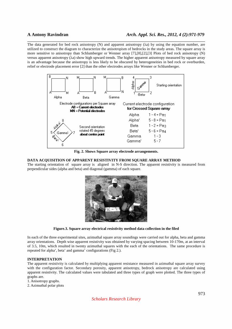
Figure.3. Square array electrical resistivity method data collection in the filed In each of the three experimental sites, azimuthal square array soundings were carried out for alpha, beta and gamma array orientations. Depth wise apparent resistivity was obtained by varying spacing between 10-170m, at an interval of 3.5, 10m, which resulted in twenty azimuthal squares with the each of the orientations. The same procedure is repeated for alpha’, beta’ and gamma’ configurations (Fig 2.). INTERPRETATION The apparent resistivity is calculated by multiplying apparent resistance measured in azimuthal square array survey with the configuration factor. Secondary porosity, apparent anisotropy, bedrock anisotropy are calculated using apparent resistivity. The calculated values were tabulated and three types of graph were plotted. The three types of graphs are. 1. Anisotropy graphs. 2. Azimuthal polar plots



3. Depth sounding graphs. ANISOTROPHY GRAPH: The calculated data of bed rock anisotropy (N) and apparent anisotropy are utilized to plot the anisotropy graphs. Anisotropy graphs are used to characterize the anisotropism of bed rocks in the study area. The plots show high upward trends. The higher apparent anisotropy is less measured by square array is an advantage because the anisotropy is likely to be obscured by heterogeneities in bed rocks or overburden. The higher anisotropy indicates that the rock formations in the study area are not symmetrical and aligned in different directions. Therefore there is high percentage of possibility of presence of groundwater in the fault zones [9],[10],[11]. Depth wise analysis of the groundwater availability and the fault / fracture trends in the study area.

y = 1.0139x3.3588

R2 = 1

0

10

20

30

40

50

0 0.5 1 1.5 2 2.5 3 3.5

Bedrock anisotropy (N)

Ap

par

ent

anis

otr

opy

(λ)

0

2

4

6

8

10

1 2


Ap

par

ent a

nis

otr

op

y (λ

)

Fig.4 a Fig.4 a

0

2

4

6

1 1.3 1.6


App

aren

t ani

sotr

opy

(λ)

Fig.4.C.

Fig. 4. Plots showing upward trends for bedrock anisotropy (N) and Apparent anisotropy (λ) measured for rocks at 4a. Mangalagiri, 4b.Chandiragiri, 4c. Kovilpatti.

AZIMUTHAL POLAR PLOTS: The apparent resistivity values calculated for the three locations are plotted as Azimuthal graphs. From these azimuthal plots in the study area three fracture directions long with homogeneous rock mass are identified on the basis of the relative of increasing order of apparent resistivity values. This fracture zone detection and rock mass identification using polar plots considerably helps to identify the groundwater level in the study area (Fig.5) The longest axis of the ellipse in the polar plot indicates maximum resistivity of the rock mass. When the polar diagram conforms to an ellipse, it is taken to represent the anisotropy. The circular pattern of the plot exhibits rock mass without fault / fracture orientation. i.e the rock is isotrophic. The intersection of the fault planes oriented in two directions assumes the cross shape. Majority of the ellipses in the location 1 are in NESW and NW SE direction and three of the single faults are in NE SW direction indicates that the fractures are oriented in NE SW direction. In the second spot fractures are oriented in E-W directions whereas in the location 3, they are directed mainly along NS direction (Table1).



Fig. 5.a

Fig. 5.b



Fig. 5.c

Fig5. Shows the pattern of Azimuthal apparent resistivity in Ohm-m plotted in different depths at 5a. Mangalagiri, 5 b.Chandiragiri, 5 c. Kovilpatti.

TABLE 1 : DEPTH AND ORIENTATION OF FRACTURES

Pattern Depth (m) and Orientation of features in

location MANGALAGIRI Depth (m) and Orientation of features in

location KOVILPATTI Depth (m) and Orientation of features

in CHANDRAGIRI

Ellipse

50 - NE SW 24.5 - NS 30 - NS 90 - EW 130 – EW 150 – E-W 100 - NW SE 42- NE-SW 110 - NE SW 120 - NW SE

Circular

80 7, 10.5,14,42, 90 140 31.5, 38.5, 42,45,49, 140 52.5,56,59.5, 63,66.5,70, 73.5,80.5,84

Single Fault

20 - NE SW 30 - NE SW 40 – NE SW 60 - EW

3.5 - N-S

10 - NE –SW 50 NE-SW 110 - NW-SE

Double fault

10 - -

The circular patterns are seen at the depth of 80 m and 140 m in location 1. circular patterns are identified in the location 2 at the depth of 80m, 140m, and 150m.



DEPTH SOUNDING Depth sounding curve is plotted between apparent resistivity and ‘A’ spacing. Plotting of ‘A’ spacing versus apparent resistivity values obtained from alpha, alpha’, beta’, beta’ orientation imply the horizontal resistivity zones. In the square array, ‘A’ spacing is equal to depth. The maximum resistivity in this area is 1275 ohm m (Fig6.).

Fig. 6.a

Fig.6b.



Fig.6.c

Fig.6. Depthwise variation azimuthal apparent resistivity vaules at 6a. Mangalagiri, 6 b.Chandiragiri, 6 c. Kovilpatti

In the plot of the 1st location, we observed that there is a sudden decreases of resistivity values at the depth of 60 m for alpha’ orientation and at the depth of 60m for beta orientation. It is an indication of the groundwater. At the depth of 100m all the resistivity curves goes to the peak and indicates the impermeable dry layer which is capable to store groundwater with granitic rock. The depth sounding plot for the 2nd location shows a rapid decrease in resistivity at the depth of 56m in alpha, alpha’ orientations. The resistivity rises at the depth of 77m for all the orientations. The existence of groundwater is observed between 77m and 180m in between the apparent resistivity value of 120Ohm.m. In the third curve the alpha, beta orientations clearly show the water table at the depth of 80.5m.

DISCUSSION AND CONCLUSION

Azimuthal Square Array (DC) Resistivity method is used to study the fracture zone of the subsurface and to investigate the groundwater level of the (Mangalagiri Village, Kovilpatti (Kalugumalai village) and Chandragiri Village) in and around Thoothukudi Area. Mangalagiri is a high anisotropy region. High anisotropy implies the presence of rocks with different physical properties in different orientations in the subsurface of the study area. Azimuthal polar plots shows that, In location 1 single faults are found between 20 - NE SW, 30 - NE SW,40 – NE SW and 60m - EW at 60m depth. Elliptical features are identified between 50m - NE SW, 90m - EW, 100m - NW SE, 110m - NE-SW. In the square array, the depth is equal to ‘A’ spacing. Plotting of depth versus apparent resistivity values obtained from alpha, alpha’, beta, beta’ orientations imply the horizontal conductivity zones . Since, the study area is situated in sedimentary and igneous rocks; the maximum recorded apparent resistivity in this terrain is 1275 Ohm-m and the resistivity range for the conductivity zone is arbitrary fixed as less than 7 Ohm-m. Horizontal fracture/permeability independent of direction and also contribution from vertical or steep fracture sets vary with azimuth creating



anisotropic distribution. The water table of the Study area Mangalagiri Water table zone 1 at a depth of 80m or 264 feet and 110m to 120m / 363 to 396 feet. Mangalagiri is a high anisotropy region. High anisotropy implies the presence of rocks with different physical properties in different orientations in the subsurface of the study area. Azimuthal polar plots shows that, In location 1 single faults are found between 20 - NE SW, 30 - NE SW,40 – NE SW and 60m - EW at 60m depth. Elliptical features are identified between 50m - NE SW, 90m - EW, 100m - NW SE, 110m - NE-SW. In the square array, the depth is equal to ‘A’ spacing. Plotting of depth versus apparent resistivity values obtained from alpha, alpha’, beta, beta’ orientations imply the horizontal conductivity zones . Since, the study area is situated in sedimentary and igneous rocks; the maximum recorded apparent resistivity in this terrain is 1275 Ohm-m and the resistivity range for the conductivity zone is arbitrary fixed as less than 7 Ohm-m. Horizontal fracture/permeability independent of direction and also contribution from vertical or steep fracture sets vary with azimuth creating anisotropic distribution. The water table of the Study area Mangalagiri Water table zone 1 at a depth of 80m or 264 feet and 110m to 120m / 363 to 396 feet. From the study on Azimuthal square array resistivity method held at Magalagiri it is concluded that fresh water is identified at a depth of 110m to 120m. The borehole drilling geological data compared with geoelectrical logging. They are obtained good freshwater from the recommended geoelectrical site at Magalagiri site. In Kovilpatti 2 single faults are detected at 3.5m - N-S depths. Elliptical features are discovered at 24.5m – NS, 130m – EW, 42m - NE-SW. The apparent resistivity displays the upper layer clay and kankar deposits identified the resistivity ranges from 7-80Ohm.m. The range of resistivity of the freshwater horizon in the profile varies from 110-124 Ohm in the intermediate layer of weathered gnessic rock. The lower part of the charnockite rock occurred in the range of resistivity ranges from 482 Ohm.m. In 3rd location of chandragiri village single faults are found between Ellipses are noticed at 30m – NS, 150m – E-W. Single fault is in-between the depth of 10m - NE –SW, 50m NE-SW. The upper layer or the first layer covered by clay and kankar deposits resistivity ranges from 7-13Ohm.m. The intermediate layer is formed by weathered gnessic rock with ground water the horizon resistivity ranges from 100-134 Ohm.m. The lower layer of granitic rock resistivity ranges from 200-489 Ohm.m.

Acknowledgement The first authors express his sincere thanks to Mr. A.P.C.V. Chockalingam, Secretary and Prof. Maragathasundaram, Principal, V.O.C. College, Tuticorin. The helps extended by Dr. N. Ramanujam, Professor and Head, Coastal Disaster Management, Pondicherry University, Andaman.

REFERENCES

[1] Busby. J.P. Geophysical Prospecting, 2000, 48:4, 677–695. [2] Darboux - Afouda, R., and Louis, P.. Geophysical Prospecting. 1989, v. 37, pp. 91-105. [3] Dobrin M.B., and Savit C.H., Introduction to Geophysical Prospecting (4thed.,),1988, McGraw – Hill, NewYork. [4] Habberjam, G.M. Geophysical Prospecting,1972, v. 20, pp. 249-266. [5] Habberjam, G.M., and Watkins, G.E. Geophysical Prospecting, 1967, v. 15, pp. 221-235. [6] Habberjam, G.M. Geophysical Prospecting.,1975, v. 23. pp. 211-247. [7] Habberjam, G.M.. Apparent resistivity observations and the use of square array techniques, in Saxov, S., and Flathe, H. (eds.). Geoexploration Monographs. series 1, 1979, no. 9, pp. 1-152. [8] Karanth K. RGroundwater assessment, development and management,1987, Tata McGraw Hill Publishing Co. Ltd. [9] Meidav T Geophysics,1960, vol. 25(5), pp 1077-1093. [10] Parasnis D. S Principles of applied geophysics, Chapman & Hall,1997,2-6 Boundary Row, London SE1 8HN, UK. [11] Reynolds J. M. An Introduction to Applied and Environmental Geophysics, 1995, John Wiley & Sons, 796 pp.

Documents

Azimuthal square array method and grounwater … an advantage because the anisotropy is less likely to be obscured by ... The longest axis of the ellipse in the polar plot indicates