AXIOMATICALLY SOUND POVERTY MEASUREMENT

WITH SCARCE DATA AND PRICE DISPERSION*

Christophe Muller**

WP-AD 2007-02

Editor: Instituto Valenciano de Investigaciones Económicas, S.A. Primera Edición Febrero 2007 Depósito Legal: V-998-2007 IVIE working papers offer in advance the results of economic research under way in order to encourage a discussion process before sending them to scientific journals for their final publication.

* I acknowledge a TMR grant from the European Union. I am grateful to the Ministry of Planning of Rwanda that provided me the data, and in which I worked from 1984 to 1988 as a technical adviser from the French Cooperation and Development Ministry. I thank participants in seminars in Oxford University, Sussex University, Nottingham University, EPGE-FG Vargas in Rio de Janeiro and at conferences IARIW98 in Cambridge, ESEM98 in Berlin, FESEM99 in Singapore, 12th World Congress of the International Economic Association in Buenos Aires for their comment. Remaining errors are mine. I am grateful for the financial support by Spanish Ministry of Sciences and Technology, Project No. SEJ2005-02829/ECON and by the Instituto Valenciano de Investigaciones Económicas. ** Departamento de Fundamentos de Análisis Económico, Universidad de Alicante, Campus de San Vicente, 03080 Alicante (Spain), E-mail: cmuller@merlin.fae.ua.es.

2

AXIOMATICALLY SOUND POVERTY MEASUREMENT WITH SCARCE DATA AND PRICE DISPERSION

Christophe Muller

ABSTRACT

We derive a parametric formula of the Watts' poverty index for the bivariate

lognormal distribution of price indices and nominal living standards. This enables us to

analyze the contributions of price and nominal living standard distributions to poverty,

to estimate poverty when only means and variances are known. We also derive a

statistical inference framework. Using data from peasants in Rwanda in four quarters, we

show that poverty estimates based on scarce information are generally not significantly

different from nonparametric estimates based on full survey information.

KEY WORDS: Measurement and analysis of poverty, Income distribution,

Personal income distribution.

JEL CLASSIFICATION: I32, O15, D31.

1. Introduction

Differences in prices across households arise from several situations. Firstly, struc-

tural adjustment plans implemented in LDCs are often challenged as entailing

poverty rises1. In particular, large movements of absolute and relative prices2,

which may be an important channel of changes in living standards. Secondly,

geographical and seasonal differences in prices that households face is a typical

feature of LDCs, generated by agricultural output fluctuations, imperfect mar-

kets, high transport and commercialisation costs, and information problems. The

World Bank (1992) presents seasonal price ratios for twenty rural developing coun-

tries in the 1980s and five products (rice, maize, wheat, sorghum, millet). The

ratios show a generally high sensitivity of agricultural prices to seasons3. These

variations imply serious consequences for poor peasants who have often limited

access to capital markets. In Africa, Baris and Couty (1981) suggest that the

seasonal price fluctuations may worsen the social differenciation. Similar evidence

1The World Bank (1990), Bourguignon, De Melo, Morrisson (1991), Sahn and Sarris(1991).

2For example, Sahn, Dorosh and Youngs (1997)) argue that in Ghana the marketliberalisation during the adjustment program of the end 1980s has lead to price decreases(or moderate increases) despite a devaluation of 100 percent. Between 1984 and 1990the prices of major staple foods fell and the rate of decline was faster than in the 1970sand early 1980s. This was accompanied by substantial changes in relative prices sinceprices of imported goods sharply rised.

3That is also well known for industrial countries in general (Riley (1961)).

3

and concern have been raised for geographical differences in prices across house-

holds. As discussed by Sen (1981), particularly in periods of famines, differences

in prices that households face can dramatically affect their entitlements relations

and their capacity to acquire food.

In these situations, poverty measures may incorporate substantial errors caused

by unaccounted large price differences across households or seasons (Jazairy, Alam-

gir and Panuccio (1992)). For example, Muller (1999a) shows for a large range

of poverty measures that local and seasonal price differences have a statistically

significant and large impact on poverty measurement in Rwanda. Then, under-

standing the contribution of the price distribution in poverty assessment, is crucial

for welfare policies.

In practice, applied price indices are generally Laspeyres or Paasche price

indices. Though, the role of price index dispersion in poverty estimation has not

been studied from a theoretical point of view. Particularly, there is no explicit

result about the price distribution contribution to poverty. The present paper

attempts to fill this lacuna by using a bivariate distribution model.

Numerous authors4, insist on the necessity of using axiomatically sound poverty

measures for inferences on poverty. One of the main axiomatically sound poverty

4e.g. Atkinson (1987).

4

measure is the Watts’ measure (Watts (1968)). We focus on this indicator and we

study three different estimators of the Watts’ measure that are based on different

requirements of empirical information, and for which we derive the asymptotic

distributions.

Are poverty estimators based on a bivariate lognormal model reliable? Can

we usefully extrapolate poverty from the sole observation of empirical means and

variances of nominal welfare and prices? The aim of this article is to answer

these questions firstly by analyzing a distribution model for prices and living

standards, secondly by deriving the asymptotic laws of poverty estimators for

statistical inference, thirdly by estimating poverty using data from Rwanda.

The situation to which the analyst is confronted is often delicate in terms of

available information. It happens that the researcher does not have access to data

collected from household surveys. Sometimes, no survey has been carried out for

the period and the region of interest. Sometimes, there has been a survey, but

the collected information has not been transferred on magnetic support and only

manual statistical treatment has been done (e.g. for historical data). Sometimes,

the survey information has been entered on tapes or diskettes, but these supports

have been lost, destroyed or are unusable. In some situations, nobody knows how

to interpret the recorded information. In other cases the data is not legally or

5

administratively available to researchers, or too costly to purchase. Finally, when

the data for the observed sample can be obtained, it is often the case that no

accurate information is available about the sampling scheme.

However, in many cases, simple statistics of the variables of interest have

sometimes been published, in particular mean and standard deviations of living

standards and price indices. Sometimes, poverty measures have been estimated

and published. Unfortunately, even in these cases the calculated poverty statistics

may not correspond to the specific needs of the researcher. Indeed, often the

published poverty measures cannot be considered as axiomatically valid from the

point of view of poverty theory5.

Even when an axiomatically sound poverty measure is used (for example a

Foster-Greer-Thorbecke measure with a severity parameter larger than two; some

Clark-Hemming-Ulph-Chakravarty measures; Watts’ measure), the estimation re-

sults can be very sensitive to the choice of the poverty line. Unfortunately, the

method for calculating the poverty line is a very contentious subject6, and poverty

statistics are generally published only for one or two lines. Then, it is unlikely

that the researcher would have chosen exactly the same poverty line and without

5 See Foster, Greer and Thorbecke (1984) and Zheng (1997) for axiomatic analysesof poverty indicators.

6See Ravallion (1998) for a detailed discussion of methods of poverty line calculation.

6

access to household level data it is impossible for her to calculate new poverty

measures with her poverty lines of interest.

We first define in section 2 the Watts’ poverty measure. Under lognormality

assumptions, we derive an expression of the Watts’ measure in terms of the para-

meters of the joint distribution of price indices and nominal living standards. We

derive in section 3, theoretical estimators of the distribution parameters and of the

Watts’ measure, as well as their asymptotic covariance matrices. In section 4, we

describe the data used in the estimation and we test the distribution assumptions.

We compare in section 5 estimates of Watts’ measures calculated using our three

estimators. Finally, section 6 concludes.

2. Watts’ poverty index

2.1. The parametric formula

The living standard indicator for household i at period t is

yit =cit

esi Iit=

wit

Iit(2.1)

where cit is the value of the consumption of household i at period t ; w it is the

standard of living of household i at date t; esi is the equivalence scale of household

7

i and I it is the price index associated with household i and period t. We denote w it

= cit/esi, the non-deflated living standard indicator (nominal living standard).

This variable is of primary empirical importance, since it corresponds to what

can be obtained from most statistical reports of household surveys, therefore from

official statistics and from many articles.

The Watts’ poverty measure (Watts (1968)) is defined as

W =

Z z

0

− ln(y/z) dµ(y) (2.2)

where µ is the cumulative density function of living standards y, and z is the

poverty line.

The Watts’ measure satisfies the focus, monotonicity, subgroup consistency,

transfer and transfer sensitivity axioms. Moreover, it is the only poverty measure

that can be written as a difference in levels of a social welfare function and that

satisfies monotonicity, continuity, decomposability and scale invariance (Zheng

(1993)). Owing to its axiomatic properties, the Watts’ measure is superior to the

head-count index (P0), or even the poverty gap index (P1).

To separate the contributions of the distribution of price indices and the dis-

tribution of nominal living standards, we now rewrite eq. 2.2 in terms of the joint

8

distribution of w and I, using the joint cumulative distribution function, F.

W =

Z ZΩ

− ln((w/I)/z) dF (w, I) (2.3)

where Ω = (w, I)| w > 0, I > 0, w/I < z. Eq. (2.3) implies that the

poverty line, z, is defined independently of the distributions of nominal living

standards and price indices. The methods for calculating poverty lines are very

varied (Ravallion (1998)), and the latter assumption may not always be satisfied.

In that case, z should be replaced by an explicit function z(F) and complementary

terms are to be added to the expressions obtained in this paper. Since no general

result can be derived for these very varied specifications, we do not pursue this

direction in this paper. In that sense, the poverty lines used in the application

must be considered as fixed values given once for all.

We shall obtain explicit expressions of contributions of non-deflated living

standards and prices by approximating F using a bivariate lognormal distribution.

The choice of the lognormal distribution is supported by the fact that histograms

of nominal living standards and price indices have unimodal asymmetrical and

leptokurtic shapes, and the observations of these variables are always positive.

The lognormal approximation has been frequently used in applied analysis of

9

living standards (e.g. Alaiz and Victoria-Feser (1990), Slesnick (1993)). In some

cases (e.g. van Praag, Hagenaars and van Eck (1983)) income data has been

found consistent with the lognormal distribution. The assumption of lognormality

of income has as well been exploited in theoretical economics (e.g. Hildenbrand

(1998)). Log-wage or log-price equations have frequently been estimated, often

implicitly relying on error terms related to normality assumptions, sometimes

asymptotically. Eaton (1980), Deaton and Grimard (1992), for example, assume

lognormality for price distributions. Other distribution models for living standards

or incomes7 or other distribution models for prices8 can also be used to represent

the data, but will not lead to an explicit expression for the Watts’ measure. In

particular, Singh-Maddala or generalised Gamma distributions are generally a

better fit for incomes than the lognormal distribution. It may also be possible

that the bivariate lognormal distribution for nominal living standards and price

indices can be significantly dominated by another distribution family.

However, the reason why we adopt a lognormal specification is not that it

corresponds to a close fit to the data, but rather because we search for a bivariate

distribution model for nominal living standards and price indices, which has the

7Champernowne (1952), Salem and Mount (1974), Kloek and van Dijk (1978), Singhand Maddala (1976), Slottje (1984), Hirschberg and Slottje (1989).

8Creedy and Martin (1994).

10

well-behaved characteristics evoked above and which leads to a parametric ex-

pression of the poverty index. Here, the question of statistical fit is secondary in

regard to the use of the distribution model as an analytical tool. The parametric

approach has been shown to be useful in poverty measurement, as demonstrated

for example in Cowell and Victoria-Feser (1996) for the treatment of data con-

tamination. Nonetheless, even in the case of imperfect statistical fit, we would

like to know if poverty estimates based on the distribution model are statistically

close to the best poverty estimates.

The Watts’ poverty measure is the only axiomatically sound poverty indicator

for which a parametric formula can be derived under bivariate lognormal distribu-

tion of price index and nominal living standard9. However, the statistical methods

that we shall implement in the following of this paper can easily be applied to

the Head-Count index, the Gini coefficient and the variance of logarithms10. To

9Owing to the presence of integrals that cannot be solved explicitly, no explicit for-mula is possible for the other known axiomatically sound poverty measures such asFoster-Greer-Thorbecke poverty indices (Pa) and Clark-Hemming-Ulph-Chakravarty’smeasures with values of poverty severity parameters consistent with the transfer axiom.

10Head-Count index and Gini income inequality measures are explicitly known wheny follows a lognormal distribution LN(m, σ2) (for example in Hammer et al. (1997)).Their formula are respectively: P0 = Φ

hln z−µ

σ

iand G= 2Φ

hσ√2

i− 1.

Parametric formulae for a few inequality indicators under income Gamma distribu-tion have also been proposed (McDonald and Jensen (1979)) or under income ParetoDistribution (Chipman (1974)).

11

shorten the exposition we focus from now exclusively on theWatts’ index. We now

present the expression of the Watts’ measure under the lognormality assumption.

Proposition 2.1. (Muller, 2006)

If nominal living standards and price indices follow a bivariate lognormal dis-

tribution law, LN

m1

m2

,

σ21 ρσ1σ2

ρσ1σ2 σ22

, then the Watts’ index is equal

to:

W = (ln z −m1 +m2).Φ

Ãln z −m1 +m2pσ21 + σ22 − 2ρσ1σ2

!

+qσ21 + σ22 − 2ρσ1σ2. φ

Ãln z −m1 +m2pσ21 + σ22 − 2ρσ1σ2

!(2.4)

where φ and Φ are respectively the p.d.f. and c.d.f. of the standard normal

distribution. The knowledge of Z = ln z−m1+m2√σ21+σ

22−2ρσ1σ2

and S =pσ21 + σ22 − 2ρσ1σ2

is sufficient to calculate W.

W = S.[Z.Φ(Z) + φ(Z)] = S.G(Z) (2.5)

by definition of G.

12

Eq. 2.4 suggests that unless all price indices are very concentrated around

1, price indices should not be neglected in the estimation of the Watts’ poverty

measure. It is also clear that the parameters associated respectively with the

distributions of w and I play similar roles. Note that m1 and σ1 (respectively m2

and σ2) are the mean and the standard deviation of the logarithms of nominal

living standards (respectively of the logarithms of price indices). To shorten, we

denote variabilities the standard deviation parameters σ1 and σ2.

Eq. 2.5 shows that the Watts’ measure can be decomposed in terms of two

sufficient statistics: S, which is the standard deviation of the logarithm of the real

living standards, that we denote global variability; and Z, which is the standardised

logarithm of the poverty line in real terms. S is equal to the variance of logarithms

and can be considered as an inequality index, although Foster and Ok (1999)

showed that it may seriously disagree with Lorenz rankings.

Φ(Z) is equal to the head-count index under the hypothesis of lognormality.

Function G(Z) is a primitive function (with value 1√2πat Z = 0) with respect

to Z of the head-count index when σ is fixed. We denote G(Z) the cumulating

poverty incidence. Consequently, the elasticity of W with respect to any inde-

pendent variable is the sum of the elasticity of the global variability and the

elasticity of the cumulative poverty incidence. The components of the gradient of

13

W with respect to parameters are ∂W∂m1

= −Φ (Z) < 0; ∂W∂m2

= Φ (Z) > 0; ∂W∂ σ1

=

σ1−ρσ2S

φ (Z) ; ∂W∂ σ2

= σ2−ρσ1S

φ (Z) ; ∂W∂ ρ

= −σ1σ2S

φ (Z) .

Some of the formulae of this paper, notably expression 2.4, can directly be

obtained by considering the distribution of real living standards y. However, it is

necessary to consider the joint bivariate distribution of (x, I) for two purposes:

1. Understanding the contribution of the distribution of each of these variables,

notably when one is concerned by levels and variabilities of prices, or by the

correlation parameter;

2. Estimating the poverty measure when only means and standard deviations

are available. Indeed, the published statistics are generally in terms of nomi-

nal living standards (typically per capita consumption, per capita income or per

adult-equivalent consumption). Very often, the mean and standard deviation of

real living standards are not published and cannot be calculated from the same

statistics for price indices and nominal living standards.

2.2. Comparison with other approaches under scarce information

What we need are only means and standard deviations of income (or living stan-

dard) and price indices (as we shall show later the correlation parameter ρ can

be set to zero with still the formula providing good results because of the gen-

14

erally weak correlation of prices and nominal living standards). Although such

information is not systematically available, it is published in a sufficient number

of cases11 to make our approach useful.

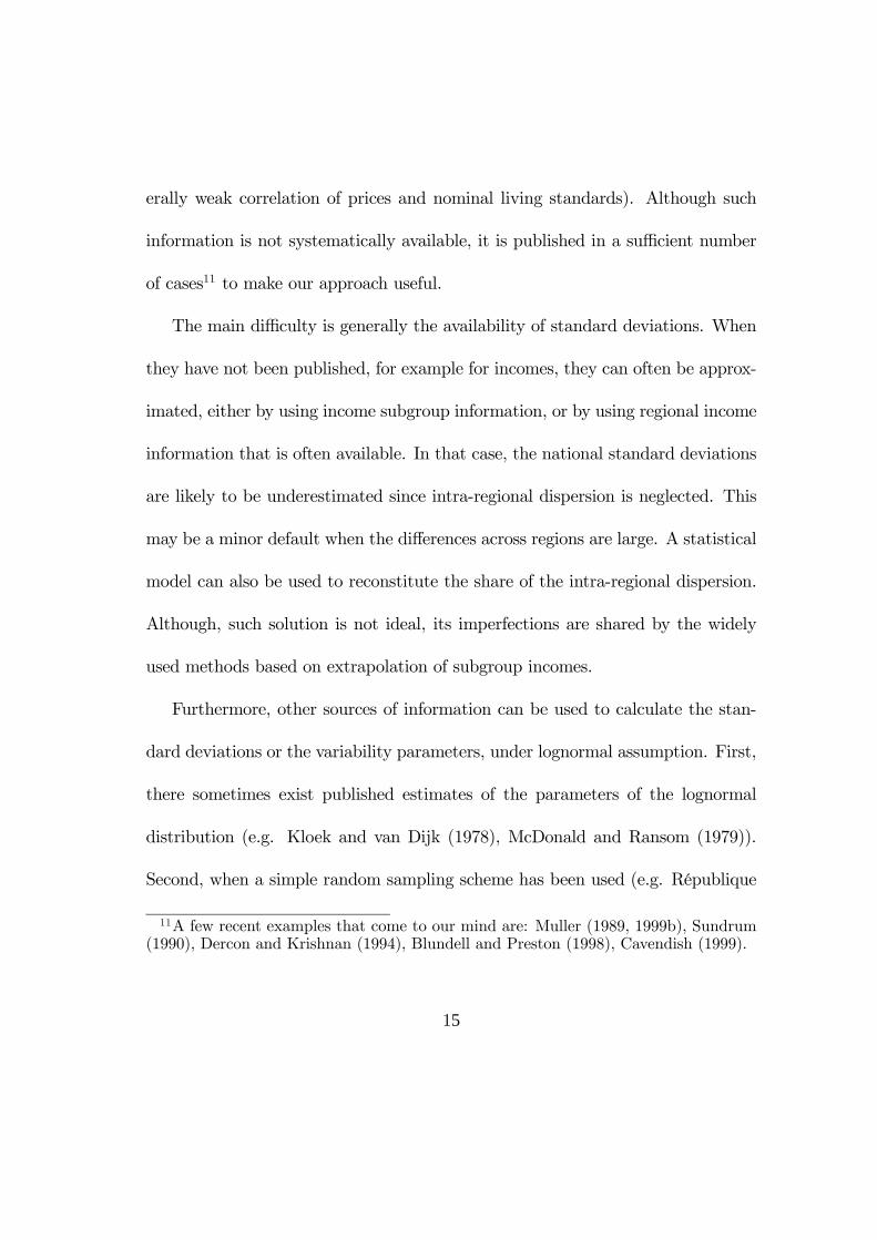
The main difficulty is generally the availability of standard deviations. When

they have not been published, for example for incomes, they can often be approx-

imated, either by using income subgroup information, or by using regional income

information that is often available. In that case, the national standard deviations

are likely to be underestimated since intra-regional dispersion is neglected. This

may be a minor default when the differences across regions are large. A statistical

model can also be used to reconstitute the share of the intra-regional dispersion.

Although, such solution is not ideal, its imperfections are shared by the widely

used methods based on extrapolation of subgroup incomes.

Furthermore, other sources of information can be used to calculate the stan-

dard deviations or the variability parameters, under lognormal assumption. First,

there sometimes exist published estimates of the parameters of the lognormal

distribution (e.g. Kloek and van Dijk (1978), McDonald and Ransom (1979)).

Second, when a simple random sampling scheme has been used (e.g. République

11A few recent examples that come to our mind are: Muller (1989, 1999b), Sundrum(1990), Dercon and Krishnan (1994), Blundell and Preston (1998), Cavendish (1999).

15

Tunisienne (1997)), the standard deviation is equal to the square root of the sam-

ple size multiplied by the standard sampling error. Then, when sampling standard

errors or confidence intervals are published, which should be a normal practice for

surveys, it may be possible to calculate the needed standard deviations. Third,

since parametric formulae for the Gini coefficient are known under lognormality,

the value of these measures can be used to recover the variability parameters when

means are known. Since published values of P0 and Gini coefficients are widely

available, our approach is likely to be applicable in many contexts.

Finally, the parametrised formulae for welfare indicators are generally provided

without the associated elements for statistical inference, i.e. the estimator and the

method for calculating confidence intervals. We stress in this paper the necessity

of providing a complete framework of statistical inference so as to ensure a proper

use of the parametrised formula for the Watts’ index. The next sections deal with

this problem.

3. Statistical Inference for the Watts’ Measure

In this section, we first discuss some estimators of the parameters of the bivariate

distribution. Then, we propose several estimators of the Watts’ poverty measure.

Finally, we propose a predictor of this measure when the price index distribution

16

changes.

3.1. MLE

We can estimate the parameters of the joint distribution by using samples of price

indices and living standards. This estimation is useful on several grounds. First,

it informs about the shape of the considered distributions. Second, it quantifies

the respective effects of both levels and variabilities of the logarithms of nominal

living standards and of the logarithms of price indices. Finally, the estimates can

be incorporated in an estimator of W. If the distributions of w and I are jointly

lognormal, then the maximum likelihood estimators (MLE) of (mi , σi), i = 1 and

2, and ρ, are consistent, asymptotically normal, efficient and invariant. under

random sampling, they are: m1 =1nΣi lnwi and m2 =

1nΣi ln Ii; σ

21 =

1nΣi (lnwi

- m1)2 and σ22 =1nΣi (ln Ii - m2)2; and ρ =

1nΣi (lnwi - m1 ).(ln Ii - m2)

σ1 σ2. Moreover, m1

and m2 are unbiased estimators.

We denote the covariance matrix of (m1 , m2 , σ1, σ2, ρ)0 as ΣL. Owing to the

invariance property of the MLE, the MLE of the Watts’ measure can be defined

using eq. 2.4 and substituting the MLEs for the distribution parameters.

Proposition 3.1. (Muller, 2006)Under random sampling, the MLE of the Watts’

measure under bivariate lognormality is:

17

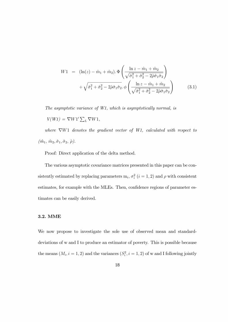
W1 = (ln(z)− m1 + m2).Φ

Ãln z − m1 + m2pσ21 + σ22 − 2ρσ1σ2

!

+qσ21 + σ22 − 2ρσ1σ2. φ

Ãln z − m1 + m2pσ21 + σ22 − 2ρσ1σ2

!(3.1)

The asymptotic variance of W1, which is asymptotically normal, is

V(W1) = ∇W10PL∇W1,

where ∇W1 denotes the gradient vector of W1, calculated with respect to

(m1, m2, σ1, σ2, ρ).

Proof: Direct application of the delta method.

The various asymptotic covariance matrices presented in this paper can be con-

sistently estimated by replacing parameters mi, σ2i (i = 1, 2) and ρ with consistent

estimates, for example with the MLEs. Then, confidence regions of parameter es-

timates can be easily derived.

3.2. MME

We now propose to investigate the sole use of observed mean and standard-

deviations of w and I to produce an estimator of poverty. This is possible because

the means (Mi, i = 1, 2) and the variances (S2i , i = 1, 2) of w and I following jointly

18

a bivariate lognormal law, can be explicitly calculated from the parameters of the

distribution. We first define estimators mi and σ2i (i = 1,2) of the distribution

parameters, using the method of moments. The MME of mi and σi (i = 1, 2) are:

σi =

vuuuutln1 +

³Mi

´2S2i

(3.2)

mi = ln(Mi)− σ2i /2 (3.3)

where M1 and S21 are respectively the empirical mean and the empirical vari-

ance of the nominal living standards, and M2 and S22 are respectively the empirical

mean and the empirical variance of the price indices.

Estimators (m1, m2, σ21, σ22) and (m1, m2, σ

21, σ

22) are both consistent, although

not asymptotically equivalent. (m1, m2, σ21, σ

22) is efficient when the actual dis-

tribution is lognormal, in contrast with (m1, m2, σ21, σ22) that is generally not

efficient.

We now define a novel estimatorW2 of theWatts’ poverty measure by plugging

the MMEs in eq. 2.4 under the hypothesis (ρ = 0). The hypothesis of non-

correlation of the logvariables, which does not modify the derivation of the formula

19

of (m1, m2, σ21, σ22), is crucial. Indeed, firstly it may often correspond to a plausible

situation. Secondly, it eliminates the need for estimates of ρ, which are typically

not available in survey publications.

Definition 3.2.

W2 = (ln z − m1 + m2).Φ

Ãln z − m1 + m2p

σ21 + σ22

!

+qσ21 + σ22. φ

Ãln z − m1 + m2p

σ21 + σ22

!(3.4)

Various combinations of parameters of the distribution are asymptotically

Gaussian with the following covariance matrices, without or with the assump-

tion that ρ = 0.

Proposition 3.3. (Muller, 2006)

The asymptotic covariance matrix of the MMEs (mj, σj)0, j = 1, 2 is

Σj = [D0j Φ

−1j Dj]

−1/N (3.5)

20

where Dj=

− e(mj+σ2j/2) −σje(mj+σ

2j/2)

−2e2mj+2σ2j −4σje2(mj+σ

2j )

and

Φj, j = 1, 2 are 2 × 2 matrices with component at row k and column l (k =

1, 2; l = 1, 2):

Φkl=p limn→+∞

©1n

Pni=1 f ik fil

ªcan be estimated by Φkl=

1n

Pni=1 f ik f il .

fik denotes the k th moment condition fk (k= 1,2) for observation i. f1 ≡ wi − em1+σ21/2

f2 ≡ w2i − e2m1+2σ21

for j = 1;

f1 ≡ Ii − em2+σ22/2

f2 ≡ I2i − e2m2+2σ22

for j = 2.

Proposition 3.4. a) The asymptotic covariance matrix of

(m1, σ1, m2, σ2)0 under the hypothesis ρ = 0 is

ΣM =

Σ1 0

0 Σ2

b) The asymptotic covariance matrix of (m1, σ1, m2, σ2)

0 is, under the hypoth-

esis ρ = 0 :

21

ΣN =

1NIF−11 0

0 Σ2

,where IF−11 is the inverse of the block of IF corresponding to (m1, σ1). IF is

the total information matrix for the whole sample of price indices and nominal

living standards.

c) V(W2) = ∇W20ΣM∇W2,

where ∇W2 is deduced from the formula of the gradient of W2 calculated at

the MMEs of the parameters.

3.3. The sampling estimator

When the survey and the sampling scheme description are available, the Watts’

measure can be directly estimated using ratios of Horwitz-Thompson estimators

(e.g. Gouriéroux (1981))12. These estimates are denoted W3 .

W3=Pn

s=1ln(ys/z)1[ys<z]

πsPns=1

1πs

where πs is the inclusion probability of household s (s

= 1,...,n). In the applied section 5, we use an estimator for sampling standard

12Alternatively, if one considers that the proper level to conduct poverty analysisis the individual one, this formula is to be modified by weighting the expression atthe numerator and denominator by the household size of household s at date t. Thisapproach has been criticised on the ground that it corresponds to equal members’ sharesof household living standard or household income. In any case, it would not change thequalitative results of this paper.

22

errors that is inspired from the method of balanced repeated replications13, which

is adapted to the actual survey (see appendix). We investigate the empirical

performance of the proposed estimators and simulators, using data from rural

Rwanda in the next sections.

4. Data and Tests

4.1. The data

Rwanda is a small rural country in Central Africa. In 1983, it was one of the

poorest country in the world, with per capita GNP of US $ 270 per annum.

More than 95 percent of the population live in rural areas (Bureau National du

Recensement (1984)).

Data for the estimation is taken from the Rwandan national budget-consumption

survey, conducted by the Government of Rwanda and the French Cooperation and

Development Ministry, in the rural part of the country from November 1982 to De-

cember 1983 (Ministère du Plan (1986a))14. 270 households were surveyed about

their budget and their consumption. Because of missing values, 256 observations

13See Krewski and Rao (1981), Roy (1984) for discussions of the properties of thistype of estimator.14The main part of the collection has been designed with the help of INSEE (French

National Statistical Institute).

23

are used in the estimation. The consumption indicators are of very high quality

(see Muller (1999a) for details).

Agricultural year 1982-83 is a fairly normal year in terms of climatic fluctua-

tions (Bulletin Climatique du Rwanda (1982, 1983, 1984)). The collection of the

consumption data was organised in four rounds, corresponding to four quarters

(A, B, C, D) of the agricultural year 1982-8315.

Table 1 shows for the year and all quarters, the mean and the standard de-

viation of per capita consumption (deflated and non-deflated) and the Laspeyres

price index.

Several studies of price surveys in Rwanda have shown the existence of substan-

tial geographical and seasonal price dispersion16. We have computed elementary

price indicators of the main categories of goods, for every quarter and every cluster

of the sample. Muller (1999a) discusses the type and the sample of prices used.

The deflation is based on Laspeyres price indices (I it) for each household and each

quarter, in which the basis is the annual national average consumption. All house-

holds in the same cluster are assumed to face the same prices. Thus, the price

index simultaneously accounts for geographical and quarterly price dispersions.

15Round A: 01/11/1982 until 16/01/1983. Round B: 29/01/1983 until 01/05/1983.Round C: 08/05/1983 until 07/08/1983. Round D: 14/08/1983 until 13/11/1983.16Niyonteze and Nsengiyumva (1986), O.S.C.E. (1987), Ministère du Plan (1986b),

Muller (1988).

24

Table 1: Mean and standard deviation of living standardsand price indices

Annual A B C DDeflatedPer CapitaConsumption

10613(5428)

2750(1701)

2702(1620)

2850(1968)

2310(1511)

Price Index1.0487(0.063)

1.1087(0.129)

0.9534(0.101)

1.0476(0.131)

1.0847(0.097)

NonDeflatedPer CapitaConsumption

10905(5355)

2995(1826)

2539(1475)

2902(1834)

2468(1524)

Standard deviations in parentheses. 256 observations.

4.2. Tests of distribution assumptions

We now turn to the tests of distribution assumptions. The lognormal assumption

introduced in Section 2 is a convenient approximation that is probably rejected by

statistical tests with some datasets. When the considered distributions are found

close to lognormality, estimator W1 will perform well. However, we also want to

explore its usefulness for distributions that are statistically distinguishable from

lognormal distributions, and to compare there W1 and W3.

To implement this exploration, we conduct several tests of lognormality as-

sumptions: Skewness-Kurtosis tests; Shapiro-Wilk tests (Shapiro andWilk (1965),

Royston (1982)); Shapiro-Francia tests (Shapiro and Francia (1972)); and Kolmogorov-

Smirnov tests. All tests are done for the quarterly and the annual per capita

nominal consumption distributions, and for the quarterly and the annual price

index distributions. The corresponding P-values are shown in Table 2.

Skewness-Kurtosis tests yield results similar to those of other tests (except

sometimes at 10 percent level for nominal living standards in period A and an-

nually). Kolmogorov-Smirnov tests, which have low power, can reject neither

the lognormality of price indices at 5 percent level at quarters A and D, nor

the lognormality of living standards at quarters A, B, C. Shapiro-Wilk (W), and

Shapiro-Francia (W’), tests yield very close results.

26

Table 2: P-values of lognormality tests

Test: 1 2 3price index in A 0.0030 0.00008 0.00062price index in B 0.0001 0.00000 0.00001price index in C 0.0000 0.00000 0.00001price index in D 0.0064 0.00016 0.00051annual per capita consumption 0.0916 0.32117 0.20879per capita consumption in A 0.0861 0.21209 0.11655per capita consumption in B 0.0431 0.01719 0.00868per capita consumption in C 0.5249 0.84615 0.52032per capita consumption in D 0.0000 0.0000 0.00001

Test: 4 5 6 7price index in A 0.364 0.0644 0.06862 0.10313price index in B 0.000 0.0207 0.00029 0.00113price index in C 0.011 0.0129 0.00073 0.00768price index in D 0.155 0.1431 0.06970 0.12212per capita consumption in A 0.816per capita consumption in B 0.163per capita consumption in C 0.934per capita consumption in D 0.028

Tests:

1: 256 households. Skewness-Kurtosis of the variable in logarithm2: 256 households. Shapiro-Wilk W of the variable in logarithm3: 256 households. Shapiro-Francia W’ of the variable in logarithm4: 256 households. Kolmogorov-Smirnov of the variable in logarithm

for N(m,σ2)

5: 90 clusters. Skewness-Kurtosis of the variable in logarithm

6: 90 clusters. Shapiro-Wilk W of the variable in logarithm

7: 90 clusters. Shapiro-Francia W’ of the variable in logarithm

We prefer the W’ test because of its better statistical properties in this context.

Its P-values imply to reject the lognormality of the price index distributions. One

might object that this result could be attributed to the clustering of observations

since all households in the same cluster are attributed the same value of the price

index. However, even when considering only one observation at the cluster level,

the lognormality of price indices is as well rejected by the W’ test, except in

quarters A and B and at 10 percent level only. Moreover, these latter outcomes

may be obtained only because of small sample size.

In contrast, the lognormality of the living standard distribution is not rejected

by the W’ test at 5 percent level, at quarters A and C, or for the year. It is

rejected at other quarters. Using different equivalent scales does not change the

test results. It is interesting to note that we dispose of a benchmark data that

does not overly determine the results of estimator comparisons with a too good

fit to lognormality.

Muller (1999b) shows the results of χ2 tests of independence between nominal

living standards and price indices that indicate at every quarter that the inde-

pendence between price indices and nominal living standards cannot be rejected.

Here, ρ = 0 would be an acceptable hypothesis.

On the whole, the preliminary tests support the adopted distribution assump-

28

tions. We are now ready to present the estimation results.

5. Estimations

In this section we compare the performances of our three poverty estimators, W1,

W2, W3. Finally, we discuss the availability of the information necessary for the

W1 and W2 calculations.

Muller (1999d) shows for six poverty lines estimates of the three estimators

W1, W2, W3, together with the sampling standard errors of W3 and the standard

errors of W1 andW2, for all quarters and the whole year. Table 3 summarizes this

information by presenting the means over the six poverty lines for these statistics.

The poverty measured using any of our indicators is unambiguously higher in

quarter D, after the dry season, than in other quarters and lower in quarter B,

after the bean harvests.

5.1. Comparison of Estimators

We now compare the quarterly and annual estimates obtained with the three es-

timators W1, W2, W3 by examining the means over the six poverty lines of their

relative variations that are shown in Table 3 as well as the means of their re-

spective standard errors. Muller (1999d) shows detailed results for all lines. It is

29

Table 3: Effects of level and variability of the logarithmof price indices

A B C D Y

r10.764(0.0244)

1.182(0.0268)

0.903(0.0108)

0.844(0.0164)

0.829(0.0238)

r20.940(0.0177)

0.943(0.0184)

0.935(0.0186)

0.982(0.00550)

0.968(0.0119)

r30.710(0.0376)

1.121(0.00527)

0.841(0.0272)

0.828(0.0211)

0.800(0.0334)

The first number in each cell is the mean over 6 poverty lines. Thenumber in parentheses is the standard deviation over the six lines.

r1 is the ratio of the Watts’ index under (m2 = 0), over the Watts indexwithout restriction;

r2 is the ratio of the Watts’ index under (σ2 = 0), over the Watts indexwithout restriction;

r3 is the ratio of the Watts’ index under (m2 = 0 and σ2 = 0), over theWatts index without restriction.

Table 4 : Watts’ Poverty indices

W3 W1 W2 (W3−W1)/W1 (W2−W1)/W1

A0.1105(0.0160)

0.1159(0.0142)

0.1095(0.0503)

−0.0476(0.00890)#

−0.0616(0.0170)#

B0.0841(0.0152)

0.0905(0.0113)

0.1023(0.0134)

−0.1811(0.265)#

0.1476(0.0434)#

C0.1091(0.0126)

0.1166(0.0143)

0.1111(0.0180)

−0.0690(0.0124)#

−0.0525(0.0143)#

D0.1861(0.0358)

0.2035(0.0201)

0.1717(0.0229)

−0.0923(0.0242)#

−0.1683(0.0464)#

Y0.0562(0.00554)

0.1445(0.00841)

0.07432(0.0118)

−0.1363(0.0634)#

0.2331(0.0805)#

The first number in each cell is the mean of W over the six povertylines. The mean over the six lines of standard errors is in parentheses.# denotes the standard deviation over the six lines.A, B, C, D denote the results of each of the quarters. Y denotes the

results based on annual per capita consumption to estimate chronicannual poverty. In the latter case, the poverty lines are multiplied byfour.

important to understand that these estimators rely on very different information

requirements. The estimation of W3 and its standard error requires the obser-

vation of the survey sample and an accurate knowledge of the sampling scheme

(not only the sampling weights). The estimation of W1 requires the observation

of the survey sample, without knowledge of the sampling scheme. The estimation

of W2 requires only the knowledge of the mean and the standard deviation for

the nominal living standard and the price index.

The estimates produced by using W1 and W3 are generally very close for

all lines and all quarters, and never significantly different at the 5 percent level

when the standard errors of W3 are considered for the test17. This is as well the

case when the standard errors of W1, σW1 , are used for the comparison. The

absolute deviation between W1 and W3 is larger in quarter D at the time of

the annual poverty crisis (-12.0 percent through -5.4 percent for different poverty

lines), although it is still non significant. Even if in other quarters too, the absolute

deviation between W1 and W3 varies with the poverty line, W1 always slightly

17Of course, and this is also true for comparisons of W3 and W2, or of W1 and W2,we could combine the standard errors associated to both estimators in the comparison.Because the standard errors of W1 and W2 are subject to the lognormality hypothesis,which is not the case for the standard error of W3, we prefer to fix the value of oneestimate and check if the sampling estimate is significantly different. This means inpractice that we check that the numbers obtained with W1 and W2 belong to theconfidence interval of our best estimate, W3.

32

overestimates poverty when compared with W3. This is consistent with a lower

tail of the distribution of real living standards that is thicker than that of a

lognormal distribution.

The comparison of W1’s andW3’s estimates shows that the distribution model

provides a reasonable approximation of poverty even if the lognormality of dis-

tributions is rejected in several periods. These results validate the model as an

analytical tool and simulation device. However, the use of W3 is limited by the

availability of the MLEs of parameters, which are not typically published. Nat-

urally, when a complete household survey dataset is available, it would generally

be inefficient to first estimate the functional form of the distribution and then use

the estimated parameters to calculate poverty measures.

Let us now turn to W2 estimates. The main interest of W2 is that when

household level data are hard to come by, or too costly to treat, using W2 could

make approximate measurement practicable. However, this is relevant only if we

can exhibit actual cases where the approximation is of sufficient quality. We first

compare withW1’s estimates. Using W2 underestimates poverty in quarters A, C,

D and the year, and overestimates poverty in quarter B. These underestimations

and overestimations are sometimes substantial18. The lower the poverty line, the

18-23.4 through -11.4 percent in quarter D following the poverty line; -4.2 through

33

greater the relative absolute deviation. The differences between W1 or W2 arise

from the gap between MLEs and MMEs of the distribution parameters and from

the assumption of a null correlation for W2.

More interesting for our purpose are the deviations between W3 and W2, i.e.

between respectively the best estimator and the estimator based on scarce infor-

mation. At the 5 % level, W1 appears to be in the confidence interval of W3 for

all quarters and all poverty lines, but not when considering annual consumption

for the calculation of poverty estimates. This latter result is related to consump-

tion smoothing occurring when using annual consumption instead of quarterly

consumption. However, at the 1 % level, W1 is in the confidence interval of W3

even when using the annual per capita consumption and with all poverty lines.

The fact that differences between W2 and W3 are generally non significant

indicates that there exist realistic situations for which the model can be used for

poverty predictions when only empirical means and standard deviations of price

indices and nominal living standards are known. Naturally, nothing ensures that

the same differences would be systematically non significant for all data sets. On

the contrary, that is certainly not the case for some surveys based on very large

-8.6 percent in quarter A; 9.8 through 21.0 percent in B; -3.6 through -7.3 percent in C;13.31 through 34.1 percent for the year.

34

sample for which the high accuracy of the estimator W3 would make it preferable

to W2. However, because there are many situations of scarce data where W3 and

W1 are impossible to calculate, and since W2 has been shown to perform well

for a national survey in a very poor country, we believe that it can be useful to

poverty study.

The relative variations between W2 or W3, and W1, provide indications about

the extent of the approximation involved in the model. Clearly, using W1 or

W2 instead of W3 changes the estimated poverty, but the estimates from the

three estimators remain close enough to provide meaningful information. This is

particularly the case when one keeps in mind the size of errors that can occur

when using non axiomatically sound indicators, when non deflating, when using

a wrong poverty line. For example, our own experience of development practice

has shown us that the number of the poor in some countries can be increased

by several times by using administrativelly chosen poverty lines rather instead of

poverty lines anchored on nutritional minima.

Finally, the distance of W2 and W1 from W3 is generally larger for quarters

in which the lognormality of nominal living standards has been rejected (B and

D). This is consistent with the restrictions imposed by the model, although the

result was not obvious a priori since the lognormality of price indices had been

35

rejected at all quarters.

5.2. The necessary information

When direct sampling estimates of poverty are not available, it seems to us that

there is little to loose by using W2. When sampling estimates of poverty are

available, but based on non axiomatically sound indicators or on inappropriate

poverty line, or without proper deflation, using W2 would provide a useful control

for fragile inferences.

The availability of mean and standard deviation of both nominal living stan-

dard and price index is crucial for the use of W2. As we said above, this informa-

tion is sometimes present in publications or can be easily reconstructed. Moreover,

limited data treatment by statistical institutes should often be sufficient to gen-

erate these statistics. In rare cases, it is even possible to know the MLEs of the

distribution parameters. Then, W1 can be used for poverty measurement.

The model used for W2 is also of interest for an univariate approach. In-

deed, in some cases, mean and standard deviation of real living standards can be

found. The formula of W can then be easily contracted with m = m1 - m2 and

σ =pσ21 + σ22 − 2ρσ1σ2, by assuming that the real living standards follow an

univariate lognormal law L(m, σ). Muller (1999c) discusses additional axiomatic

36

properties of the Watts’ measure in this case. The methods used in this paper

can therefore be readily adapted. Another context where one may want to use

this univariate approach is when there is no information at all about prices and

that one is ready, or constrained, to neglect completely the price index dispersion

in poverty measurement.

Finally, rarer information is necessary for the calculation of the asymptotic

covariance matrices for W1 and W2. However, under the assumption ρ = 0, which

may be frequently satisfied in practice, simplifications occur and only estimators

of σ1 and σ2 are necessary beyond the sample moments of variables. Again,

the MMEs given by eq. 3.2 can be used. Therefore, in favorable cases, while

still with scarce information, not only an axiomatic sound poverty measure can

be estimated, but also the accuracy of its estimation, as long as one accepts the

lognormality approximation.

6. Conclusion

Available statistical information for poverty analysis is often quite limited when it

is impossible to access data collected from household survey. Nonetheless, in such

situations, the mean and standard deviation of living standards and price indices of

37

the variables of interest are sometimes published. In some cases, poverty measures

have been estimated, but the calculated poverty statistics do not correspond to

the researcher’s requirements.

Moreover, large geographical and temporal differences in prices exist in agri-

cultural developing countries because of market imperfections and high output

seasonality. They may also occur during structural adjustment periods, or be-

cause of weather, economic or political shocks that are frequent in LDCs. Unfor-

tunately, price differences across households and periods seriously affect poverty

measurement.

We propose in this article a simultaneous solution to the data availability

problem and the price dispersion problem. Using a bivariate lognormal model

of the distributions of price indices and nominal living standards, we derive a

parametric formula of the Watts’ poverty measure and its associated statistical

inference framework.

We show that this formula can be useful for three tasks, which we illustrate

using national data from Rwanda, a very poor African country:

1. Analyzing the interactions of price indices and nominal living standards for

poverty analysis.

2. Deriving estimates of an axiomatically sound poverty measure (and of its

38

accuracy), which accounts for price dispersion and for any desired poverty line,

from the sole knowledge of the mean and standard deviation of price indices and

nominal living standards.

39

APPENDICES:

Proof of Proposition 3.6:

Under ρ = 0, the two distributions of w and I are independent since those of

lnw and ln I are. Then, cov(m1, m2) = cov(m1, σ2) = cov(σ1, m2) = cov(σ1, σ2)

= 0.

For one observation, the block IF−11 =

σ21(1− ρ2) 0

0ρ4.(σ1−σ2)2+4σ21σ22+ρ2(4σ21σ22−2σ21−2σ22)

σ41.(2σ22+ρ

2.(1−ρ2).(−1+σ22))

since IF is diagonal for ρ = 0.

The variance of W2 is obtained by application of the delta method. []

BIBLIOGRAPHY

ALAIZ, M.P. and M.-P. VICTORIA-FESER, ”Modelling Income Distribution in

Spain: A Robust Parametric Approach”, Distributional Analysis research Programme,

Working Paper no 20, LSE-STICERD, June 1996.

ATKINSON, A.B., ”On the Measurement of Poverty”, Econometrica, vol. 55, n. 4,

749-764, July 1987.

BARIS, P. And P. COUTY, ”Prix, marchés et circuit commerciaux africains”,

AMIRA No 35, December 1981.

BAYE, M.R., ”Price Dispersion and Functional Price Indices”, Econometrica, Vol.

53, No. 1, January 1985.

40

BLUNDELL, R. and I. PRESTON, ”Consumption Inequality and Income Uncer-

tainty”, The Quarterly Journal of Economics, May 1998.

BOURGUIGNON, F., de MELO, J. and C. MORRISSON, ”Poverty and Income

Distribution During Adjustment: Issues and Evidence from the OECD Project”, World

Development, vol. 19, No. 11, 1485-1508, 1991.

BULLETIN CLIMATIQUE DU RWANDA, ”Climatologie et Précipitations”, Kigali,

1982, 1983, 1984.

BUREAU NATIONAL DU RECENSEMENT, ”Recensement de la Population du

Rwanda, 1978. Tome 1: Analyse.”, Kigali, Rwanda, 1984.

CAVENDISH, W., ”Poverty, inequality and environmental resources: quantitative

analysis of rural households”, Working Paper CSAE 99.9, 1999.

CHIPMAN, J.S., ”The Welfare Ranking of Pareto Distributions”, Journal of Eco-

nomic Theory, 9, 275-282, 1974.

CREEDY, J. and V.L. MARTIN, ”A Model of the Distribution of Prices”, Oxford

Bulletin of Economics and Statistics, 56, I, 1994.

DEATON, A. and F. GRIMARD, ”Demand Analysis for Tax Reform in Pakistan”,

Working Paper Princeton University research program in Development Studies, January

1992.

DERCON, S. and P. KRISHNAN, ”Poverty in Rural Ethiopia 1989-94”, Discussion

41

paper CSAE, October 1994.

EATON, J., ”Price Variability, Utility and Savings”, Review of Economic Studies,

XLVII, 513-520, 1980.

FOSTER, J., J. GREER and E. THORBECKE, 1984, ”A Class of Decomposable

Poverty Measures”, Econometrica, vol. 52, n. 3, May.

FOSTER, J. and E.A. OK, ”Lorenz Dominance and the Variance of Logarithms”,

Econometrica, Vol. 67, No. 4, 901-907, July 1999.

GOURIEROUX, C., ”Théorie des Sondages”, Economica, Paris, 1981.

GOURIEROUX, C. and A. MONFORT, ”Statistique et Modèles Econométriques”,

Economica, 1989.

HAMMER, L., G. PYATT, H. WHITE, N. POUW, ”Poverty in sub-Saharan Africa.

What can we learn from the World Bank’s Poverty Assessments?”, Institute of Social

Studies, The Hague, November 1997.

HILDENBRAND, W., ”How Relevant are specifications of Behavioral Relations on

the Micro-Level for Modelling the Time Path of Population Aggregates”, Rheinische

Friedrich-Wilhelms-Universitat Bonn, Projekbereich A, Discussion paper No. A-569.

HIRSCHBERG, J.G. and D.J. SLOTTJE, ”Remembrance of Things Past the Dis-

tribution of Earnings across Occupations and the Kappa Criterion”, Journal of Econo-

metrics, 42, 121-130, 1989.

42

JAZAIRY, I., M. ALAMGIR and T. PANUCCIO, ”The State of World Rural

Poverty”, Intermediate Technology Publications, 1992.

JOHNSON, N.L. and S. KOTZ, ”Distributions in Statistics: Continuous Multivari-

ate Distributions”, John Wiley & Sons, Inc., 1973.

KLOEK, T. and H. K. VAN DIJK, 1978, ”Efficient Estimation of Income Distribu-

tion Parameters”, Journal of Econometrics, 8, 61-74.

KREWSKI, D., and J.N.K., RAO, ”Inference from Stratified Sample”, Annals of

Statistics, vol. 9, pp 1010-1019, 1981.

McDONALD, J. B. and B. C. JENSEN, 1979, ”An Analysis of Some Properties of

Alternative Measures of Income Inequality Based on the Gamma Distribution Func-

tion”, Journal of the American Statistical Association, December, Volume 73, 856-860.

MINISTERE DU PLAN, ”Méthodologie de la Collecte et de l’échantillonnage de

l’Enquête Nationale sur le Budget et la Consommation 1982-83 en Milieu Rural”, Kigali,

1986.

MINISTERE DU PLAN, ”Enquête des Prix PCI au Rwanda”, Kigali, 1986.

MULLER, C., ”E.N.B.C.: Relevés de prix en milieu rural”, Ministère du Plan,

Kigali, Rwanda, 1988.

MULLER, C., ”Structure de la consommation finale des ménages ruraux au Rwanda”,

Ministère de la Coopération et du Développement, Paris, 1989.

43

MULLER, C., ”The Measurement of Dynamic Poverty with Geographical and In-

tertemporal Price Dispersion”, Working Paper CREDIT, University of Nottingham,

June 1999a.

MULLER, C., ”The Spatial Association of Price Indices and Living Standards”,

Working Paper CREDIT, Nottingham University, July 1999b.

MULLER, C., ”The Properties of the Watts’ poverty Index under Lognormality”,

Discussion Paper No. 99/36, University of Nottingham, December 1999c.

MULLER, C., ”The Watts’ Poverty Index with Explicit Price Variability”, Discus-

sion Paper No. 99/32, University of Nottingham, November 1999d.

MULLER, C., ”Poverty Simulations and Price Changes," Forthcoming Korean Jour-

nal of Economics, 2006.

NIYONTEZE, F. And A. NSENGIYUMVA, ”Dépouillement et présentation des

résultats de l’enquête sur marchés Projet Kigali-Est”, Projet Kigali-Est, Juin 1986.

O.S.C.E., ”Note statistique rapide sur la comparaison des niveaux des prix du

Rwanda”, Bruxelles, 1987.

RAVALLION, M., ”Poverty Lines in Theory and Practice”, Living Standards Mea-

surement Study Working Paper No. 133, July 1998.

REPUBLIQUE TUNISIENNE, Ministère du Développement Economique, ”Enquête

nationale sur le Budget, la Consommation et le Niveau de Vie des Ménages - 1995.

44

Volume A: Résultats de l’enquête sur le budget des ménages”, Institut National de la

Statistique, Tunis, Décembre 1998.

RILEY, H.E., ”Some aspects of Seasonality in the Consumer Price Index”, American

Statistical Association Journal, March 1961.

ROYSTON, J.P., ”An Extension of Shapiro and Wilk’s W Test for Normality to

Large Samples”, Applied Statistics, No. 2, pp 115-124, 1982.

SAHN, D.E. and A. SARRIS, ”Structural Adjustment and the Welfare of Rural

Smallholders: A Comparative Analysis from Sub-Saharan Africa”, The World Bank

Economic Review, Vol. 1, No. 2, 1991.

SAHN, D.E., P.A. DOROSH, S.D. YOUNGER, ”Structural Adjustment Reconsid-

ered”, Cambridge University Press, 1997.

SALEM, A. B. Z. and T. D. MOUNT, ”A Convenient Descriptive Model of Income

Distribution: The Gamma Density”, Econometrica, Vol. 42, No. 6, November 1974.

SEN, A., ”Poverty and Famines”, Clarendon Press, Oxford, 1981.

SHAPIRO, S.S. and R.S. FRANCIA, ”An Approximate Analysis of Variance Test

for Normality”, Journal of American Statistical Association, March 1972.

SHAPIRO, S.S. and M.B. WILK, ”An analysis of variance test for normality (com-

plete samples), Biometrika, 52, p. 591-611, 1965.

SINGH, S.K. and G.S. MADDALA, ”A Function for Size Distribution of Incomes”,

45

Econometrica, Vol. 44, No. 5, 1976.

SLOTTJE, D.J., ”A Measure of Income Inequality in the U.S. for the Years 1952-

1980 based on the Beta Distribution of the Second Kind”, Economics Letters, 15, 369-

375, 1984.

SUNDRUM, R.M., ”Income Distribution in Less Developed Countries”, Routledge,

London, 1990.

TOWNSEND, R.M., ”Risk and Insurance in Village India”, Econometrica, vol. 62,

No 3, 539-591, May 1994.

VAN PRAAG, B., A. HAGENAARS and W. VAN ECK, 1983, ”The Influence

of Classification and Observation Errors on the Measurement of Income Inequality”,

Econometrica, Vol. 51, No. 4, July.

WATTS, H.W., ”An Economic Definition of Poverty” in D.P. Moynihan (ed.), ”On

Understanding Poverty”, 316-329, Basic Book, New York, 1968.

THE WORLD BANK, ”World Development Report 1990. Poverty”, Oxford Uni-

versity Press, 1990.

THEWORLD BANK, ”World Development Report 1992”, Oxford University Press,

1992.

ZHENG, B., ”An axiomatic characterization of the Watts poverty index”, Economic

Letters, 42, 81-86, 1993.

46

ZHENG, B., ”Aggregate Poverty Measures”, Journal of Economic Surveys, Vol. 11,

No. 2, 1997.

47