Embed Size (px)
Citation preview

From:OECD Journal: Economic Studies
Access the journal at:http://dx.doi.org/10.1787/19952856
Avoiding debt trapsFiscal consolidation, financial backstops and structural reforms
Pier Carlo Padoan, Urban Sila, Paul van den Noord
Please cite this article as:
Padoan, Pier Carlo, Urban Sila and Paul van den Noord (2012),“Avoiding debt traps: Fiscal consolidation, financial backstops andstructural reforms”, OECD Journal: Economic Studies, Vol. 2012/1.http://dx.doi.org/10.1787/eco_studies-2012-5k8xbnjbn9hl

This document and any map included herein are without prejudice to the status of orsovereignty over any territory, to the delimitation of international frontiers and boundaries and tothe name of any territory, city or area.
OECD Journal: Economic Studies
Volume 2012
© OECD 2013
151
Avoiding debt traps:Fiscal consolidation, financial
backstops and structural reforms
by
Pier Carlo Padoan, Urban Sila
and Paul van den Noord*
In this article we develop a simple and stylised analytical framework, which is bothtractable and feasible to estimate, capturing several key dimensions of the sovereigndebt crisis in Europe. We use it to examine if and how a combination of fiscalconsolidation, structural reform and financial backstops can help countries, notablythe southern euro-area countries, to escape from the debt trap. Our analysisconfirms that the loss of fiscal policy space in countries trapped in bad dynamicsinevitably requires that fiscal action be directed towards consolidation despite someoutput loss in the short run. In particular, reducing debt levels breeds strongergrowth and results in lower sovereign risk premia. We identify also a veryimportant role for structural reform to help countries escape from bad dynamics.Last but not least, we find that financial backstops are helpful, but only to “buytime”. This additional time must be used productively, for fiscal consolidation andstructural reforms to bear fruit as well as to make progress with institutionalreforms of the European monetary union.
JEL classification codes: E62, C33, C62
Key words: Fiscal policy, sovereign debt, multiple equilibria
* OECD Economics Department: e-mail contacts [email protected]; [email protected] authors are indebted to two referees for comments and suggestions and to Penny Elghadab andLyn Urmston for editorial support. The views expressed in this article are those of the authors anddo not necessarily reflect those of the OECD or the governments of its member countries.

AVOIDING DEBT TRAPS: FISCAL CONSOLIDATION, FINANCIAL BACKSTOPS AND STRUCTURAL REFORMS
OECD JOURNAL: ECONOMIC STUDIES – VOLUME 2012 © OECD 2013152
In the current macroeconomic environment economies may find themselves trapped in a
“bad equilibrium”. One often hears the case made of periphery countries in the euro area
being in such a “bad equilibrium”, characterised by the simultaneous occurrence of, and
adverse feedbacks between, high and growing fiscal deficits and debt, high risk premia on
sovereign debt, slumping economic activity and plummeting confidence. Remedies to
break the downward spiral and escape debt traps generally include financial firewalls to
prevent contagion and structural reforms to boost growth. The role of fiscal policy is less
clear; whereas consolidation may help to put debt on a sustainable path, negative demand
effects may, on the other hand, generate offsets and could exacerbate the downturn,
adding to the risk premiums, and thus deepen the “bad equilibrium”.1
These general mechanisms on their own are well understood, but how they interact in
a consistent dynamic setting is less clear. In this article we provide a simple analytical
framework to fill this gap. We develop a simple version of a model with two solutions – a
stable and an unstable one – combining a negative relationship between debt and growth
inspired by the seminal work of Reinhart and Rogoff (2010) and the government’s
inter-temporal budget constraint. We extend this model to make it more realistic by adding
the effects of fiscal policy and interest rates on growth and by introducing an interest rate
equation. We estimate the core parameters of the model and use the estimates to identify,
empirically, the two solutions and then simulate the policies that can help a country
caught in bad debt and growth dynamics to recover. This model embeds three relevant sets
of policy variables in a monetary union: structural reform, fiscal consolidation and the use
of financial backstops to reduce sovereign bond yields.
We start with a brief account of stylised developments since the onset of the crisis. We
then elaborate the theoretical model, report the estimation results of a panel regression
analysis and finally examine the comparative static and dynamic responses to fiscal,
structural and financial policies. The final section concludes.
1. A brief review of the main issuesOver the past few years, even prior to the outbreak of the global financial crisis, new
stylised facts have emerged in the macroeconomic environment. Public debt has grown
significantly in almost all advanced economies. Partly this was a consequence of the drop
in public revenues caused by the recession, and partly it was due to large public efforts,
especially in some countries, to deal with banking crises. This has generated a negative
feedback on growth with the possibility of a vicious circle of high debt, low growth and
unsustainable public debt dynamics. Fragility has spilled over to banks which hold
substantial amounts of sovereign debt in their balance sheets, especially in the euro area.
This has, in turn, weighed negatively on confidence as the risk of a possible twin crisis
affecting sovereign debt and credit markets simultaneously has become more significant.
As has become painfully obvious, confidence can affect growth significantly. Simulations
by the OECD (2011) point to a chain of causation which goes from confidence (in both

AVOIDING DEBT TRAPS: FISCAL CONSOLIDATION, FINANCIAL BACKSTOPS AND STRUCTURAL REFORMS
OECD JOURNAL: ECONOMIC STUDIES – VOLUME 2012 © OECD 2013 153
business and household) to financial markets, and next to the real economy. This
relationship can affect growth positively or negatively and it can lead to significant
differences in performance.
The increased role of confidence in driving macroeconomic performance suggests that
we are operating in a world of multiple solutions, both stable and unstable. These may
result in a strong overreaction of markets, especially in the euro area where national
banking woes and sovereign stress are strongly intertwined. Take interest rates on
sovereign bonds for example (Figure 1). After the crisis of the EMS in 1992, and in the run
up to monetary union, these converged significantly and spreads practically disappeared
for a number of years. After the outbreak of the crisis, markets overreacted in the opposite
direction amplifying risk assessment and contributing to the emergence of vicious circles
and a fragmentation of monetary and financial markets along national lines.
More generally, in OECD economies, for quite some time, markets have underpriced
risk and favoured excessive risk taking including in private debt accumulation. During the
so-called great moderation in the United States they have fuelled credit and housing
booms and strengthened the perception that private debt was, after all, sustainable. An
indication of this is the persistence of a negative interest rate-growth rate differential for
OECD economies (Turner and Spinelli, 2011). In the euro area, this general pattern has
taken the form of the expansion of current account (saving-investment) imbalances (OECD,
2012a) which was fed largely through the banking sector, unsustainable investment, and
housing booms in deficit countries and the outflow of capital from surplus countries.
Eventually – triggered by the financial crisis that erupted in the United States – booms
turned to bust and the financial system in Europe ran into serious trouble, taking
sovereigns down in its wake.
Dealing with such a situation is posing severe policy challenges. The loss of fiscal
policy space inevitably requires that fiscal action is directed towards consolidation.
Benefits of fiscal consolidation are long term, as reducing debt levels breeds stronger
Figure 1. Sovereign bond yields in the euro area(monthly averages, 10-year maturities)
Source: OECD Analytical Database.
30
25
20
10
15
5
0
IRL ITA PRTDEU ESP FRA GRC
Jan.
1992
Oct. 19
92
July
1993
Apr. 19
94
Jan.
1995
Oct.
1995
July
1996
Apr.
1997
Jan.
1998
Oct.
1998
July
1999
Apr.
2000
Jan.
2001
Oct. 20
01
July
2002
Apr.
2003
Jan.
2004
Oct.
2004
July
2005
Apr.
2006
Jan.
2007
Oct.
2007
July
2008
Apr.
2009
Jan.
2010
Oct.
2010
Apr.
2012
July
2011

AVOIDING DEBT TRAPS: FISCAL CONSOLIDATION, FINANCIAL BACKSTOPS AND STRUCTURAL REFORMS
OECD JOURNAL: ECONOMIC STUDIES – VOLUME 2012 © OECD 2013154
growth, but also short term, to the extent that credible fiscal consolidation programmes
may boost market confidence which translates into lower risk premia. However, in the
short term the negative impact on demand may adversely affect market confidence to the
extent that it depresses growth and hence debt sustainability. In practice, which of the two
effects of fiscal consolidation prevails is an empirical issue largely dependent on the size of
the fiscal multiplier.
Monetary policy in many advanced economies has reached the zero bound and, since
the crisis, monetary authorities have introduced “unconventional” measures to deal with
the recession. The balance sheets of major central banks have expanded accordingly
(Figure 2). However, in a situation of financial fragility where disequilibria may spiral out of
control, monetary authorities can fulfil an additional function with respect to supporting
economic activity (in a framework of price stability and anchored inflation expectations),
the “lender of last resort” function which can include both sovereign debt and credit
markets. Such provision of a financial backstop is particularly relevant in situations in
which, like the euro area crisis, contagion effects can be very significant and affect several
channels at the same time.
The available policy toolkit also includes structural reforms. Structural reforms, which
consist of a large number of different measures, can have a significant impact on growth
(OECD, 2012a), but the benefits of growth require time to materialise in full.
Since the beginning of the crisis many countries have enacted structural reforms,
often in tandem with fiscal consolidation measures (OECD, 2012b). This bodes well for the
future, but time may be too short for the benefits of structural reforms to materialise and
for markets to appreciate such improvements and translate them into lower risk premia. If
markets are patient, debt sustainability would be easier and favourable dynamics could be
set in motion where lower risk premia and higher growth reinforce each other. But if
markets are impatient, such good dynamics may never be feasible. Rather, bad dynamics,
characterised by higher risk premia and lower growth, may prevail, leading countries
towards explosive debt.
Figure 2. Central bank liabilities (in local currency)
Source: Federal Reserve; Bank of Japan; European Central Bank.
3 500
3 000
2 000
1 500
2 500
1 000
500
United States (bn dollars) Euro area (bn euros) Japan (100 bn yen)
Jan.
2007
July
2007
Jan.
2008
July
2008
Jan.
2009
July
2009
Jan.
2010
July
2010
Jan.
2011
July
2011
Jan.
2012
July
2012
AVOIDING DEBT TRAPS: FISCAL CONSOLIDATION, FINANCIAL BACKSTOPS AND STRUCTURAL REFORMS
OECD JOURNAL: ECONOMIC STUDIES – VOLUME 2012 © OECD 2013 155
This calls for co-ordinated action where available policy tools, fiscal, financial, and
structural policies must operate in co-ordination to allow economies to move towards a
high-growth and low-debt equilibrium. What such a co-ordinated solution might look like
is the subject of the rest of this article.
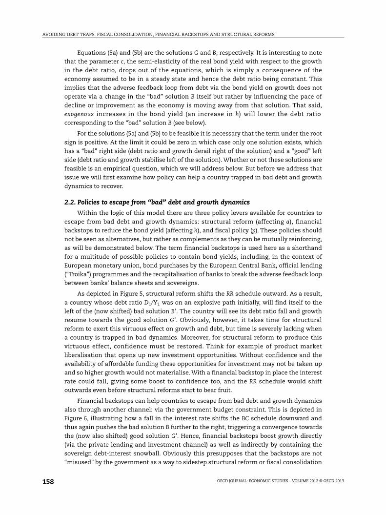
2. A simple model of growth and debtIn this section we provide a simple yet consistent analytical framework to analyse the
interactions described in the previous section. It is inspired by a model developed by
Duesenberry (1958) to analyse the Great Depression which had many characteristics
similar to the current situation. We start off with the exposition of the model, which we
subsequently use to analyse the stabilisation properties of three policy levers: structural
reforms, financial backstops and fiscal consolidation.
2.1. Assumptions and specification
The model has three equations. The first equation describes a negative relationship
between public debt and economic growth (Y = output, D = real government debt and an
over-dot indicates the change in the variable):
(1a)
This equation is depicted in Figure 3 as the downward-sloping straight line RR. RR
stands for Reinhart and Rogoff (2010) who have recently tested this relationship
empirically. This negative relationship can be explained, inter alia, by adverse expectations
with regard to future taxation associated with high public debt. It may also capture the
effect of sovereign stress spilling over to banks which hold substantial amounts of
sovereign debt on their balance sheets, in turn weighing negatively on the cost of financing
for the private sector and on confidence and growth. Growth is positively affected by the
Figure 3. “Good” and “bad” growth and debt dynamics
Note: The horizontal axis measures the public debt to GDP ratio and the vertical axis the growth rates of public debtand output. RR is the relationship between growth and debt and BC the government’s budget constraint. If the debtratio is located right from the intersection B, it derails while output growth falls at an accelerating pace. Left of B thedebt ratio converges towards G.
YY
a bDY
=
G
B
BC
RR
DY
YY
DD
. .
,
D0 /Y0 D1/Y1

AVOIDING DEBT TRAPS: FISCAL CONSOLIDATION, FINANCIAL BACKSTOPS AND STRUCTURAL REFORMS
OECD JOURNAL: ECONOMIC STUDIES – VOLUME 2012 © OECD 2013156
exogenous impact of structural reforms captured by parameter a. To keep the model
simple we abstract from inflation, hence real and nominal variables are identical, and we
also ignore potential output.
Growth equation (1a) can be augmented with the impact on growth of financial
conditions (to the extent this is not already captured by the debt ratio) proxied by the (real)
interest rate r, and the fiscal policy stance proxied by the primary deficit as a share of GDP p:2
(1b)
According to this relationship, a higher interest rate depresses growth and a larger
fiscal deficit supports (and by extension fiscal consolidation weakens) growth, with the
associated semi-elasticities represented by the parameters f and g, respectively. These are
just the first-order effects of interest rates and fiscal policy on growth. There are
second-order effects that run through the government’s budget constraint, which is the
second equation of the model and in fact an identity. It relates the primary deficit as a per
cent of GDP p to the interest rate r and public debt D:
(2a)
Dividing the two sides of the equation by D yields:
(2b)
This is the hyperbolic relationship between real growth of debt and the debt ratio depicted
as BC (as in budget constraint) in Figure 3.3 As the debt ratio increases, the real growth of
debt approaches asymptotically the real interest rate. If the debt ratio is located in the
interval between points G and B (for example at a level indicated by D0/Y0), output growth
will exceed the growth of debt, and hence the debt ratio is falling until point G (for “good”
dynamics) is attained: this is a stable steady state. However, if the debt ratio is located to
the right of point B (e.g. if the debt ratio equals D1/Y1), the growth of debt exceeds output
growth. Beyond the point B (indicating “bad” dynamics) debt keeps growing while output
growth keeps falling, hence the debt ratio is on an explosive path.
What is not shown in Figure 3 (for the sake of simplicity) is that if the debt ratio is on
an explosive path the real interest rate is bound to increase, thus adding momentum to the
debt explosion. To capture this effect we need to introduce an interest rate equation, which
is the third equation of our stylised model. Specifically, we assume that the interest rate
responds to the growth in the debt ratio and an (exogenous) factor h. Therefore:
(3)
The rationale for including the growth rate of the debt ratio as an explanatory variable
is that we see this as a good measure of the sustainability of public finances. Specifically,
we expect an accelerating debt ratio to raise the probability of default (for real or as
perceived by the markets), i.e. the faster the increase in the debt ratio, the higher the risk
premium. The parameter h under normal circumstances represents long-term neutral
interest rates, but in stress situations also captures the impact of swings in market
sentiment and contagion effects (in as much as these are unrelated to local debt dynamics)
as well as financial backstops to offset such sentiment and contagion effects. These
components will be disentangled in the estimated version below. As we shall see these
factors seem to play an important role in the recent euro area sovereign debt dynamics.
YY
a bDY
fr gp= +
D rD pY= +
DD
rp
D Y= +
/
r h cDD
YY
= +

AVOIDING DEBT TRAPS: FISCAL CONSOLIDATION, FINANCIAL BACKSTOPS AND STRUCTURAL REFORMS
OECD JOURNAL: ECONOMIC STUDIES – VOLUME 2012 © OECD 2013 157
In sum, our model points to three potentially explosive feedback mechanisms:
i) between the debt ratio and growth; ii) between the debt ratio and the interest rate; and
iii) between growth and the interest rate. Specifically, a high debt ratio depresses growth,
which in turn boosts the debt ratio, etc., a high interest rate pushes up debt which gives a
higher interest rate, etc., and a higher interest rate depresses growth which pushes up the
debt ratio and hence the interest rate, etc. These feedbacks will be explosive if the initial
debt ratio is “right of B” or converge (to the “good” solution G) if it is located “left of B”.
It is possible to derive formal expressions for the debt positions that correspond to the
solutions G and B, but before we do so we need to address an important technical
consideration. The negative correlation between debt and growth has been explained in
different ways (Cecchetti et al., 2012, Elmeskov and Sutherland, 2012, Reinhart and Rogoff,
2010 and others), but there is evidence that debt ratios negatively affect growth only beyond
a certain threshold. Therefore, the RR schedule may be “kinked”, as depicted in Figure 4. The
empirical literature following Reinhart and Rogoff’s seminal paper generally finds the debt
threshold to be close to 90% of GDP.4 Indeed this is what we find also in our own empirical
work (see below). This does not change the basic features of the model, other than that the
value of the parameter b in equation (1b) is conditional on the level of the debt ratio.
Ignoring this consideration for now, the steady-state debt ratio (when debt and output
grow at the same rate) can be derived by equating the BC and RR equations (1b) and (2b) and
equating the growth rates of debt and output in the interest equation (3), which yields:
(4)
This has two solutions:
(5a)
(5b)
Figure 4. Debt threshold
G
B
BC
RR
DY
YY
DD
. .
,
+ + +( ) =bDY
a gp f hDY
p2
1 0
DY
a gp f h a gp f h bp
b
G
=+ +( ) + +( )1 1 4
2
2
DY
a gp f h a gp f h bp
b
B
=+ +( ) + + +( )1 1 4
2
2
AVOIDING DEBT TRAPS: FISCAL CONSOLIDATION, FINANCIAL BACKSTOPS AND STRUCTURAL REFORMS
OECD JOURNAL: ECONOMIC STUDIES – VOLUME 2012 © OECD 2013158
Equations (5a) and (5b) are the solutions G and B, respectively. It is interesting to note
that the parameter c, the semi-elasticity of the real bond yield with respect to the growth
in the debt ratio, drops out of the equations, which is simply a consequence of the
economy assumed to be in a steady state and hence the debt ratio being constant. This
implies that the adverse feedback loop from debt via the bond yield on growth does not
operate via a change in the “bad” solution B itself but rather by influencing the pace of
decline or improvement as the economy is moving away from that solution. That said,
exogenous increases in the bond yield (an increase in h) will lower the debt ratio
corresponding to the “bad” solution B (see below).
For the solutions (5a) and (5b) to be feasible it is necessary that the term under the root
sign is positive. At the limit it could be zero in which case only one solution exists, which
has a “bad” right side (debt ratio and growth derail right of the solution) and a “good” left
side (debt ratio and growth stabilise left of the solution). Whether or not these solutions are
feasible is an empirical question, which we will address below. But before we address that
issue we will first examine how policy can help a country trapped in bad debt and growth
dynamics to recover.
2.2. Policies to escape from “bad” debt and growth dynamics
Within the logic of this model there are three policy levers available for countries to
escape from bad debt and growth dynamics: structural reform (affecting a), financial
backstops to reduce the bond yield (affecting h), and fiscal policy (p). These policies should
not be seen as alternatives, but rather as complements as they can be mutually reinforcing,
as will be demonstrated below. The term financial backstops is used here as a shorthand
for a multitude of possible policies to contain bond yields, including, in the context of
European monetary union, bond purchases by the European Central Bank, official lending
(“Troika”) programmes and the recapitalisation of banks to break the adverse feedback loop
between banks’ balance sheets and sovereigns.
As depicted in Figure 5, structural reform shifts the RR schedule outward. As a result,
a country whose debt ratio D1/Y1 was on an explosive path initially, will find itself to the
left of the (now shifted) bad solution B’. The country will see its debt ratio fall and growth
resume towards the good solution G’. Obviously, however, it takes time for structural
reform to exert this virtuous effect on growth and debt, but time is severely lacking when
a country is trapped in bad dynamics. Moreover, for structural reform to produce this
virtuous effect, confidence must be restored. Think for example of product market
liberalisation that opens up new investment opportunities. Without confidence and the
availability of affordable funding these opportunities for investment may not be taken up
and so higher growth would not materialise. With a financial backstop in place the interest
rate could fall, giving some boost to confidence too, and the RR schedule would shift
outwards even before structural reforms start to bear fruit.
Financial backstops can help countries to escape from bad debt and growth dynamics
also through another channel: via the government budget constraint. This is depicted in
Figure 6, illustrating how a fall in the interest rate shifts the BC schedule downward and
thus again pushes the bad solution B further to the right, triggering a convergence towards
the (now also shifted) good solution G’. Hence, financial backstops boost growth directly
(via the private lending and investment channel) as well as indirectly by containing the
sovereign debt-interest snowball. Obviously this presupposes that the backstops are not
“misused” by the government as a way to sidestep structural reform or fiscal consolidation

AVOIDING DEBT TRAPS: FISCAL CONSOLIDATION, FINANCIAL BACKSTOPS AND STRUCTURAL REFORMS
OECD JOURNAL: ECONOMIC STUDIES – VOLUME 2012 © OECD 2013 159
(to which we turn next). Furthermore, it is also important that the financial backstop is set
up in a way that moral hazard is contained; otherwise the confidence bridge provided by
the financial backstop breaks down.
These findings can be formalised by computing the relevant policy multipliers from
equation (5b):
(6)
(7)
These equations confirm the graphical analysis: structural reform and financial backstops
help a country to escape from bad debt and growth dynamics (as they “shift the bad
solution to the right”). Importantly, these multipliers also confirm that these policies are
mutually reinforcing: a rightward shift in the “bad” solution triggered by structural reform
raises the multiplier of financial backstops and vice versa.
In our stylised model fiscal consolidation works via two channels – output and the
government budget constraint. This is similar to financial backstops, which work through
the same channels, except that the effects of fiscal consolidation are in opposite directions,
with the net effect ambiguous. Fiscal consolidation is represented by a sustained cut in the
primary deficit p, which shifts the BC schedule down as depicted in Figure 7. However, as
shown in Figure 8 it also implies a negative demand shock, shifting the RR schedule down.
The former is potentially stabilising (the bad solution shifts to the right) whereas the latter
is potentially destabilising (the bad solution shifts to the left).
It is again possible to derive the relevant multiplier to measure the impact of changes
in the primary deficit p on the bad solution, which reads:
(8)
Whether an increase in the primary deficit gives a lower bad debt ratio (beyond which
the economy becomes unstable) or the reverse is indeed ambiguous and depends on the
initial level of the bad solution and on the “Keynesian” fiscal demand multiplier g. When
both are large, such that , fiscal expansion (an increase of p) will have a
favourable impact on the bad solution i.e. it will shift it to the right. This is a situation
where the country has fiscal space available to effectively boost the economy out of bad
debt and growth dynamics through fiscal expansion. But if either of the two is small (the
Keynesian fiscal impact on growth is small and the initial bad solution for the debt ratio is
small, for instance, because the country suffers from a bad reputation in financial markets
as gauged by a high value of the parameter h), such that , fiscal expansion will
exacerbate the bad dynamics trap. Fiscal consolidation is then the appropriate policy,
possibly in combination with structural reform and financial backstops (since these
increase the multiplier (8) and hence the effectiveness of fiscal consolidation).
=+ +( )
>DY
aDY
a gp f h bp
B B
/1
1 40
2
=+
+ +( )<
DY
hDY
f
a gp f h bp
B B
/1
1 40
2
=+ +( )
>DY
p gDY
a gp f h bp
B B
/ 11
1 42
00
gDY
B
> 1
gDY
B
< 1

AVOIDING DEBT TRAPS: FISCAL CONSOLIDATION, FINANCIAL BACKSTOPS AND STRUCTURAL REFORMS
OECD JOURNAL: ECONOMIC STUDIES – VOLUME 2012 © OECD 2013160
Where exactly the bad solution ends up after fiscal consolidation is thus an empiricalquestion: our theory cannot predict this. There is a vast though inconclusive literature onthe subject, prompted by Giavazzi and Pagano (1990) who argued that fiscal consolidationscan be expansionary, based on a number of case studies. According to Perotti (1999) theodds of an expansionary effect of fiscal consolidation increase with the extent of the initialfiscal predicament, in line with our finding that the initial position of the “bad debt ratio”matters for the stabilisation properties of fiscal policy. SVAR modelling work by Tenhofen,Heppke-Falk and Wolff (2011) yields evidence of a strong positive growth impact of publicinvestment, but other fiscal shocks are found to have very little net impact on growth.However, more recently there have been additional views and evidence that the fiscaldemand multiplier may be positive and large (of the order of one or more), and fiscalconsolidation destabilising, at least in depressed economies (see, for example, De Long andSummers, 2012 and IMF, 2012).
Figure 5. The impact of structural reform and financial backstopsthrough the output channel
Figure 6. The impact of financial backstops through the governmentbudget channel
G
G’
BB’
BC
RR’
DY
YY
DD
. .
,
D1/Y1
GG’
B
B’
BC’
BC’
RR
DY
YY
DD
. .
,
D1/Y1

AVOIDING DEBT TRAPS: FISCAL CONSOLIDATION, FINANCIAL BACKSTOPS AND STRUCTURAL REFORMS
OECD JOURNAL: ECONOMIC STUDIES – VOLUME 2012 © OECD 2013 161
To sum up, the effect of fiscal policy on the growth path of the economy is ambiguousand strongly depends on the initial conditions. It is therefore of crucial importance toempirically calibrate the model so as to be able to assess the need for, and effectiveness of,fiscal consolidation alongside other policy tools when countries are trapped by bad debtand growth dynamics. We turn to this in the sections below.
3. Panel estimatesIn this section we report estimation results for the growth and interest rate equations
(1b) and (3) which we will use as the basis for simulations of both shocks and policyresponses in the next section. The data for GDP growth, public debt, primary deficit,interest rates and control variables are obtained from the OECD Economic Outlook 90Database. More details on the variables used can be found in the Data Annex. Theestimations are based on a sample of 28 OECD countries and data spans for up to 52 years,from 1960 to 2011.5 We use annual data.
Figure 7. The impact of fiscal consolidation through the governmentbudget channel
Figure 8. The impact of fiscal consolidation through the output channel
G
G’
B
B’
BC
BC’
RR
DY
YY
DD
. .
,
D1/Y1
G
G’
B
B’
BC
RRRR’
DY
YY
DD
. .
,
D1/Y1

AVOIDING DEBT TRAPS: FISCAL CONSOLIDATION, FINANCIAL BACKSTOPS AND STRUCTURAL REFORMS
OECD JOURNAL: ECONOMIC STUDIES – VOLUME 2012 © OECD 2013162
We purposefully use as broad a sample as possible, in order not to make results
dependent on an arbitrarily chosen period or group of countries. However, in this way the
sample is unbalanced: for some countries the data go back to the 1960s, whereas for others,
it only goes back to the 2000s. The exact composition of the panel also depends on the
estimation method due to a different use of lags. If characteristics of countries with a shorter
series differ in a systematic way, having an unbalanced panel may result in a sample bias,
but we nevertheless think that having a larger and longer sample brings about important
benefits. In any case, in our empirical approach we at all times control for country fixed
effects, taking much of this problem away. Moreover, when we test the robustness of our
results to shortening the time period, the conclusions remain largely unaltered.
3.1. The growth equation
We estimate the following equation:
(9)
where , i denotes a country and t denotes time. All the main variables of
interest are expressed in per cent or percentage points. The dependent variable is
n-year forward-overlapping moving average of annual real GDP growth rates, between
year t+1 and t+n. Varying the future time span allows us to distinguish between potentially
differing short-term and medium/long-term effects of the explanatory variables on
growth. We set n to 1, 3 and 5. This approach also partly addresses the problem of
endogeneity due to reverse causality and simultaneity between GDP growth, public debt
and primary deficit. Whereas we claim that debt and primary deficit affect growth, it may
also be the case that low growth leads to increases in public debt and primary deficit via
automatic stabilisers and induced policy reactions. Therefore, by keeping the two policy
variables at time t and moving the growth rate forward in time, endogeneity is weakened.
Similar measures of growth have been used in Checherita and Rother (2010) and Cecchetti
et al. (2011). In addition, our preferred specification rests on instrumental variable
estimation so as to address any remaining endogeneity.
The term in equation (9) represents public debt as a share of GDP, which in the
third term on the right-hand side is interacted with a dummy variable M, indicating
whether the public debt is above the threshold T. This recognises the fact that the effect of
debt on growth may be non-linear. In order to avoid a discrete jump in the estimated
regression line at the point where public debt equals the threshold, T is subtracted. This
ensures that the growth equation is kinked like the one depicted in Figure 4. The and
measure the primary deficit as a share of (lagged)6 GDP and the real long-term interest
rate on government bonds, respectively. stands for country-fixed effects and for
time-fixed effects.
Finally, stands for a vector of controls. Here we follow the growth regressions literature
and include a standard set of controls as, for example, reported in Barro and Sala-i-Martin
(2004) to capture conditional convergence. It is important to note, however, that our approach
gD
YM
D
YT
Pi t n
i t
i ti t debt T
i t
i t
i,
,
,, ;
,
,*+ >= + + +1 2
,,
,,
’, ,
t
i ti t i t i t i tY
r X+ + + + +1
gn
Y
Yi t nk
ni t k
i t k,
,
,+
=
+
+=
1
1 1
gi t n, +
D
Yi t
i t
,
,
P
Yi t
i t
,
, 1
ri t,
i t
Xi t,

AVOIDING DEBT TRAPS: FISCAL CONSOLIDATION, FINANCIAL BACKSTOPS AND STRUCTURAL REFORMS
OECD JOURNAL: ECONOMIC STUDIES – VOLUME 2012 © OECD 2013 163
differs from standard growth regressions in that we use GDP growth as opposed to per capita
GDP growth as the dependent variable. This is done in order to be consistent with the model
presented in Section 2. Nevertheless, we include population growth and GDP per capita as
controls, which essentially boils down to an analogous specification.
The controls in our case include: inflation rate to control for macroeconomic stability;
the logarithm of the initial GDP per capita, to control for the catching up effect; investment
(gross capital formation) as a share of GDP to measure capital formation and to serve as a
proxy for the saving rate; mean years of schooling to measure human capital; trade openness
measured as the sum of total exports and imports as a share of GDP; population growth and
the dependency ratio to control for the evolution of labour supply; and a banking crisis
indicator, to control for potential negative effects on growth in years of banking crises as
predicted by Reinhart and Rogoff (2009).
The banking crisis variable is based on the data on systemic banking crises constructed
by Laeven and Valencia (2008 and 2010).7 In constructing the banking crisis indicator we
follow Cecchetti et al. (2011); it takes a value of zero if in the subsequent n years there is no
banking crisis, and the value of 1/n, 2/n, and so forth, if a banking crisis occurs in one,
two, etc., of the subsequent n years. The banking crisis indicator is, therefore, the only
regressor which is not predetermined with respect to the future average growth rate.
Table 1 reports the estimation results for three different averages of future GDP growth
rates: five-year forward average, three-year forward average and a one-year forward growth
rate. In columns (2), (4) and (6) we report fixed effects results. Due to the overlapping nature
of our dependent variable, the error term follows a moving-average process, therefore we
use a robust procedure to compute the standard errors of our coefficient estimates; the
standard errors are also clustered by country. Despite the future growth rate on the
left-hand side, there may still be endogeneity bias remaining if the growth rate and
sovereign debt are jointly determined by a third, omitted variable. Therefore, in columns
(1), (3) and (5) we report the results from the instrumental variable GMM estimation,
implemented in stata by the xtivreg2 of Schaffer (2010). To instrument for the sovereign
debt ratio and primary deficit ratio, we use their 1-3 period lags. Reported standard errors
are robust to heteroskedasticity and autocorrelation of the order 5, 3 or 2, in columns (1), (3)
or (5), respectively. GMM IV is our preferred specification, and is also used later in the
simulations of the model for policy analysis. The reported fixed-effects estimation results
primarily serve as a robustness check.
At the bottom of the Table 1 we list the estimated threshold effect. This is the level of
debt where the kink in the growth equation appears. The estimation procedure of the
threshold follows Hansen (1999); for each specification we search over a grid of different
thresholds to find the one that minimises the residual sum of squares. We then take the
estimated threshold effect as given, and use it to estimate the model. The estimated
threshold effects in all cases are close to 90%, consistent with findings by other
researchers. Reinhart and Rogoff (2010) find that for the level of debt ratio above 90%, the
average growth rate falls, whereas below that threshold, the relationship between
government debt and GDP growth is weak. A point estimate for the threshold close to 90%
for the effect of public debt on growth is also reported in Cecchetti et al. (2011) and
Checherita and Rother (2010). Kumar and Woo (2010), on the other hand, consider two
externally-imposed thresholds at 30% and 90% debt levels, and they find that beyond the
90% level, debt becomes harmful to growth.

AVOIDING DEBT TRAPS: FISCAL CONSOLIDATION, FINANCIAL BACKSTOPS AND STRUCTURAL REFORMS
OECD JOURNAL: ECONOMIC STUDIES – VOLUME 2012 © OECD 2013164
According to the results reported in Table 1 the effect of government debt below the
threshold is not statistically significant, except perhaps in the short term as indicated in
column (5). Above the threshold, on the other hand, the effect is consistently negative and
statistically significant, shown in italics towards the bottom of Table 1. First, comparing the
coefficients across different specifications one can note that the negative effect of debt on
growth becomes stronger over time, that is, the coefficient in column (5) is smaller in
absolute value than that in column (1). Therefore, increasing public debt by 1 percentage
point this year will on average reduce GDP growth next year by 0.012 percentage points,
whereas it will reduce the average annual growth over the next five years by 0.028 percentage
points. The effect of debt on growth in the latter case is therefore about twice as large.
Table 1. Estimated growth equations
Dependent variable
(1) (2) (3) (4) (5) (6)
GMM IV FE GMM IV FE GMM IV FE
Five year forwardof GDP growth rate (%)
Three year forwardof GDP growth rate (%)
One year forwardof GDP growth rate (%)
Government debt/GDP (%) -0.000271 -0.000546 0.00204 -0.000555 0.0135* 0.00213
(0.00493) (0.00775) (0.00563) (0.00762) (0.00710) (0.00741)
Governmentdebt and thresholddummy -0.0274*** -0.0276** -0.0269*** -0.0285*** -0.0258*** -0.0293***
– interaction (0.00818) (0.0122) (0.00874) (0.0103) (0.00963) (0.00898)
Primary deficit/lagged GDP (%) 0.0116 0.0177 0.0389 0.0239 0.0596 0.0105
(0.0201) (0.0213) (0.0263) (0.0265) (0.0405) (0.0335)
Real long-term interest rate -0.0611*** -0.0288 -0.122*** -0.0954** -0.216*** -0.155**
(0.0235) (0.0264) (0.0335) (0.0406) (0.0447) (0.0577)
Inflation rate (%) -0.0571** -0.0483 -0.119*** -0.110*** -0.236*** -0.206***
(0.0241) (0.0325) (0.0275) (0.0376) (0.0431) (0.0524)
Log of GDP per capita -9.333*** -8.876*** -9.241*** -8.758*** -6.825*** -6.388***
(0.863) (1.090) (0.944) (1.081) (1.270) (1.046)
Gross fixed capital formation/GDP (%) -0.0605*** -0.0609* -0.0492* -0.0674* 0.0236 -0.0146
(0.0224) (0.0297) (0.0295) (0.0339) (0.0398) (0.0385)
Mean years of schooling -0.0688 -0.0974 -0.247 -0.231 -0.587*** -0.483**
(0.186) (0.252) (0.197) (0.233) (0.216) (0.232)
Trade openness 0.0143** 0.0159* 0.0180** 0.0182* 0.0313*** 0.0214**
(0.00686) (0.00881) (0.00717) (0.00923) (0.00927) (0.0102)
Population growth (%) -0.303 -0.244 -0.402 -0.436 -0.0652 0.0100
(0.228) (0.259) (0.255) (0.294) (0.256) (0.257)
Total dependency ratio -0.0359* -0.0338 -0.0477* -0.0389 -0.0320 0.0102
(0.0216) (0.0244) (0.0248) (0.0259) (0.0312) (0.0258)
Banking crisis indicator -1.659*** -1.765*** -1.771*** -1.778*** -1.645*** -1.644***
(0.325) (0.399) (0.330) (0.395) (0.399) (0.460)
Year dummies Yes Yes Yes Yes Yes Yes
Constant 162.5*** 162.9*** 119.9***
(18.49) (18.59) (18.02)
Effect of government debt/GDP (%) -0.0277*** -0.0281*** -0.0249*** -0.0291*** -0.0123* -0.0271***
– above threshold (p-value) (0.000) (0.005) (0.000) (0.001) (0.061) (0.000)
Observations 640 699 696 755 749 808
Number of countries 28 28 28 28 28 28
Debt threshold 91 91 86 86 82 87
Note: *** p < 0.01, ** p < 0.05, * p < 0.1. All regressions use country-fixed effects. Instrumental variables in GMM IVregressions [columns (1), (3) and (5)] are 1-3 period lags of government debt ratio and primary deficit ratio. In GMM IVregressions the reported standard errors are robust to heteroskedasticity and autocorrelation of the order 5, 3 or 2, incolumns (1), (3) or (5), respectively. In fixed-effects panel regressions [columns (2), (4) and (6)] the reported standarderrors are robust to heteroskedasticity and adjusted for clusters by countries.

AVOIDING DEBT TRAPS: FISCAL CONSOLIDATION, FINANCIAL BACKSTOPS AND STRUCTURAL REFORMS
OECD JOURNAL: ECONOMIC STUDIES – VOLUME 2012 © OECD 2013 165
The direction of the effects of the primary deficit and the interest rate on growth is
also as expected and the longer-run effects are generally weaker than the short-run
effects. However, in all cases the effects are statistically not significant, suggesting that
these effects are, if anything, weakly positive. Increasing the primary deficit as a share of
lagged GDP by 1 percentage point this year increases the growth rate by 0.060 percentage
points in the next year, as reported in column (5). This drops down to 0.039 for the average
growth rate in the next three years, column (3), and to 0.012 over the next five years,
column (1)8. In the same way, the real long-term sovereign interest rate has a stronger
negative effect on growth in the short term as compared with the medium/long term.
Table 1 also reports the results for other controls. The coefficient of the log of GDP per
capita has a negative sign, implying the so called “catch-up” effect. The inflation rate has a
negative effect on GDP growth and trade openness has a positive effect, both as expected.
A strong and negative effect on growth comes from the banking crisis indicator. For
example, a banking crisis one year ahead is expected to reduce the growth rate in that
same year by about 1.6 percentage points, as reported in column (5). The rest of the
coefficients on controls are statistically not significant. The population (total dependency
ratio and population growth) and education variables are slow-moving hence, perhaps in
the fixed effects setting, they do not have enough variation. Recall also, that in our case we
use GDP growth on the left-hand side instead of per capita GDP growth, therefore, when we
compare the coefficient on population growth with other growth regression estimations
we should subtract 1 from our result. Doing so, we get somewhat closer to the results
reported in Checherita and Rother (2010). The coefficient on investment (gross fixed capital
formation) is also not statistically significant, but insignificant coefficients for this variable
are reported in similar regressions also by Cecchetti et al. (2010) and Checherita and Rother
(2010).
3.2. Interest rate equation
We estimate the following interest rate equation:
(10)
where, the dependent variable measures the one year forward real long-term interest
rate on government bonds, i denotes a country and t denotes time. and stand for
country-fixed effects and year dummies, respectively, and is the error term. Again, all
the main variables are expressed in per cent or percentage points.
The second term on the right-hand side in equation (10) represents the growth rate of
the debt to GDP ratio. As suggested in the theoretical section above, we would expect the
long-term sovereign interest rate to increase when debt dynamics worsen. We use the
current debt dynamics to estimate the effect on future interest rates. Moving the interest
rate one year forward partly solves the problem of simultaneity, given that the current
interest rate can have quite a strong impact on current debt dynamics. However, as
stressed also by Laubach (2009), it is the expectations of future debt dynamics that are
important for determining the interest rate, and can also be used to circumvent the
problem of endogeneity. He for example uses projections of fiscal variables several years
into the future to estimate the interest rate equation. However, to stick to the model as
presented in Section 2, we use the current level of debt growth. Expectations about debt
rD
D
Y
YWi t
it
i t
i t
i ti t i t i t,
,
,
,
’, ,+ = + + + + +1
1 1
ri t, +1
i t
i t,

AVOIDING DEBT TRAPS: FISCAL CONSOLIDATION, FINANCIAL BACKSTOPS AND STRUCTURAL REFORMS
OECD JOURNAL: ECONOMIC STUDIES – VOLUME 2012 © OECD 2013166
dynamics are thus incorporated into the country-fixed effect and the error term. Of course,
in this way the error term remains correlated with the debt growth term, therefore we
again estimate the model using instrumental variable GMM estimation.
The in equation (10) stands for the controls. In choosing the controls we follow
Laubach (2009) and Checherita et al. (2010) that estimate similar equations. The real
short-term interest rate controls for the effect of monetary policy and monetary conditions
more generally on long-term interest rates; the inflation rate controls for macroeconomic
stability and rises in prices, and the measure of trade openness allows for the open economy
and controls for potential effects of openness on capital flows and interest rates.
On top of this we also include two additional sets of controls. First is the banking crisis
indicator variable and the interaction of the banking crisis indicator with the “southern
eurozone” dummy. The “southern eurozone” indicator variable is equal to one for the
following countries: Greece, Ireland, Italy, Portugal, Slovakia, Slovenia and Spain; and
zero otherwise, from the year they adopted the euro. The second set of controls includes,
in addition to the debt growth variable, the interaction of the debt growth with the “southern
eurozone” dummy.
The rationale for including these variables comes from the discussion in De Grauwe
and Ji (2012). They observe that the increase in the debt-to-GDP ratios since 2007 is
significantly faster in the United States and the United Kingdom than in the eurozone, yet
it is the eurozone that has experienced a severe sovereign debt crisis. They argue that this
is because the eurozone countries do not have control over their own money. Thereby,
member countries are susceptible to movements of distrust. When such movements of
distrust occur, the sovereign spreads are likely to increase significantly without much
movement in the underlying “fundamentals” that influence the solvency of the country. In
their paper they find that while before the crisis the debt-to-GDP ratios in the eurozone do
not seem to have affected the spreads, after 2008, this relationship becomes quite
significant, i.e. it appears that financial markets are less tolerant towards high debt-to-GDP
ratios in the eurozone as compared with the stand-alone countries, and especially so in the
eurozone periphery. Evidence discussed in Section 1 is consistent with this view.
To capture this phenomenon we therefore include the banking crisis dummy and
interact it with the southern eurozone dummy to see whether in the time of crisis, the
sovereign yields in the “southern eurozone” increase more than predicted by fundamentals.
On the other hand, the interaction of the debt growth variable with the “southern
eurozone” indicator measures whether changes in debt growth have stronger consequences
for the “southern eurozone” compared with the rest of the OECD countries.
In Table 2 we report the results from the fixed-effects panel estimation, column (2),
and the instrumental variables GMM estimation, column (1), our preferred specification.9
Instrumental variables used in column (1) are the 1-3 period lags of government debt ratio
growth and interactions. The reported standard errors are robust to heteroskedasticity and
autocorrelation.
The reported effect of the growth of government debt to GDP ratio on long-term real
interest rates in column (1) is of a positive sign, as expected. A rise in debt growth by
1 percentage point increases the next year real long-term interest rate by 6.3 basis points
for countries that do not belong to the “EMU south” group. The interaction of the debt
growth with the south eurozone dummy shows that for these countries movements in debt
have a much larger effect on interest rates compared with the rest of the OECD.
Wi t,

AVOIDING DEBT TRAPS: FISCAL CONSOLIDATION, FINANCIAL BACKSTOPS AND STRUCTURAL REFORMS
OECD JOURNAL: ECONOMIC STUDIES – VOLUME 2012 © OECD 2013 167
Interestingly, the banking crisis by itself does not have a statistically-significant impact on
the long-term sovereign interest rate, although in the sense of economic significance, the
coefficient is quite large. More importantly, however, there is evidence that for the
southern euro countries, the banking crisis causes significant stress and, on average, adds
about 180 basis points more to the interest rate compared with other countries in times of
banking crisis. The results are therefore telling a story that the southern euro area
countries in times of banking crisis are, for reasons not related to “fundamentals”, put
under higher market pressure and at the same time they need to pay the higher price for
any increases in their debt growth. This is evidence for the behaviour of markets as
described by De Grauwe and Ji (2012).
4. Policy experimentsThe econometric estimates reported in the previous section allow us to identify the
empirical values of the parameters in the theoretical model. Once we have empirically
estimated the parameters we are able to compute the debt levels that correspond to the
“good” and “bad” solutions as well as the multipliers developed in Section 2 (comparative
statics). In addition, we are able to set up a dynamic version of the model in discrete time,
and use it to run shock and policy simulations (comparative dynamics).
Table 2. The effect of growth in sovereign debt on long-term interest rates
(1) (2)
GMM IV FE
Dependent variable: One year forward real long-term interest rate
Growth in government debt ratio (%) 0.0628** 0.0159**
(0.0263) (0.00669)
Interaction – debt growth and EMU “south” indicator 0.103*** 0.0148
(0.0329) (0.0216)
Banking crisis indicator -0.126 0.388
(0.393) (0.310)
Interaction – banking crisis and EMU “south” 1.855* 2.844***
(0.976) (0.926)
EMU “south” indicator 0.431 0.0459
(0.379) (0.646)
Real short-term interest rate 0.161*** 0.274***
(0.0482) (0.0909)
Inflation rate (%) -0.261*** -0.281***
(0.0422) (0.0769)
Trade openness 0.0129 0.00256
(0.00957) (0.0121)
Year dummies Yes Yes
Constant 1.872**
(0.736)
Observations 772 821
Number of countries 29 29
Note: GMM IV regressions. *** p < 0.01, ** p < 0.05, * p < 0.1. Standard errors are in parentheses. All regressions usecountry-fixed effects and we include year dummies. In GMM IV regression the instrumental variables are 1-3 periodlags of government debt ratio growth and its interaction terms. The reported standard errors are robust toheteroskedasticity and autocorrelation of order 2, respectively. In the fixed effects panel regression the reportedstandard errors are robust to heteroskedasticity and adjusted for clusters by countries.

AVOIDING DEBT TRAPS: FISCAL CONSOLIDATION, FINANCIAL BACKSTOPS AND STRUCTURAL REFORMS
OECD JOURNAL: ECONOMIC STUDIES – VOLUME 2012 © OECD 2013168
4.1. Comparative statics
Most parameter values in our stylised model can be directly inferred from the
estimation results, with the exception of the terms a and h appearing in, respectively, the
growth and interest rate equations. These comprise country-specific constant terms as
well as the impact of a range of control variables on growth and the interest rate, and hence
vary across countries and over time. In addition we need to modify the theoretical model
to capture the threshold effect of public debt on growth. Specifically, the relevant growth
equation reads:
(1c)
where M is a dummy variable taking the value 1 if the debt ratio is above the threshold and
zero otherwise and b2 represents the difference in the growth impact of the debt ratio
above the threshold, T. This equation can be re-written as:
(1d)
in which . This gives us a properly adjusted estimate of the constant term in
the equation. The debt threshold, i.e. the level of debt where the kink in the growth
equation appears, is fixed at 82% of GDP, consistent with our regression results for the
GMM IV results for the one-year forward growth equation (our preferred specification).
The numerical parameters inferred from the estimation results, are reported in
Table 3. The baseline parameters refer to the parameters excluding the impact of financial
crisis and/or the country being part of the “euro area south” in the interest rate equation.
The second column in the table presents the parameters that apply to countries in the euro
area south whose bond yields and growth rates are affected by the banking and sovereign
debt crisis. In line with the regression results, the parameter a is reduced by 0.016 to
capture the estimated impact of the banking crisis on growth. Similarly, the parameters c
and h are increased by 0.103 and 0.019 to capture the stronger impact of, respectively,
growth in the debt-to-GDP ratio and the banking crisis.
These parameter estimates allow us to identify the “good” and “bad” debt ratios and
the multipliers developed in Section 3. It should be stressed, however, that these estimates
apply to the average of the sample as a whole and not necessarily to individual countries
or sub-periods, and obviously are surrounded by uncertainty margins. The results are
reported in Table 4. For a primary deficit (p) equalling 0.3% of GDP (which is the sample
Table 3. Model parameters
Whole sample pre-crisis “Euro area south” crisis
a 0.028 0.012
b1 -0.013 -0.013
b2 0.026 0.026
c 0.063 0.166
f 0.216 0.216
g 0.060 0.060
h 0.027 0.046
Note: In the calibrated model fractions are not expressed aspercentages, meaning that intercepts of the estimated growth andinterest-rate equations are divided by 100.
YY
a bDY
b MDY
T fr gp= +1 2
YY
a b b MDY
fr gp= +( ) +’ 1 2
a a b M T’ = + ×2

AVOIDING DEBT TRAPS: FISCAL CONSOLIDATION, FINANCIAL BACKSTOPS AND STRUCTURAL REFORMS
OECD JOURNAL: ECONOMIC STUDIES – VOLUME 2012 © OECD 2013 169
average), the corresponding sample average “bad” debt ratio equals 107% of GDP. This
implies that, on average, a country recording a debt ratio above 107% would see its debt
ratio spiral out of control and its economy slump in the absence of offsetting policy action.
Conversely, the “good” solution to which the debt ratio converges if it is below the 107%
threshold turns out to be 69% of GDP. This means that if the debt ratio is in the 69%-107%
interval it would, on average, be falling towards 69% (and conversely increasing towards
69% if it is below that level). Again, these are rough orders of magnitude based on estimates
that apply exclusively to the sample average, and for illustrative purposes only.
The multiplier analysis in Table 4 shows that, again for the sample as a whole, structural
reform yielding a sustained increase in economic growth of 0.1 percentage points per annum
raises the bad debt ratio (i.e. moves out the point B) by 10 percentage points. This suggests
that the contribution structural reforms brings to debt sustainability can be significant.
Similarly, a sustained cut in the risk premium on the interest rate by 10 basis points
increases the bad debt ratio by 12 percentage points. A sustained increase in the primary
deficit as a share of GDP by 0.1 percentage point reduces the bad debt ratio (beyond which
bad dynamics set in) by 8 percentage points. This means that, based on our sample and time
period, fiscal expansion, on average, renders the economy less stable. The consequence is
that a country caught in bad dynamics should pursue a restrictive fiscal policy.
Table 4 also reports a sensitivity analysis for different assumptions with regard to the
estimated model parameters. We have computed the impact of increases or decreases
amounting to one standard error for several parameters. The most striking finding is the
large sensitivity of the results to variations in the parameter value for b2, the semi-elasticity
(interaction term) of growth with respect to the debt ratio beyond the “Reinhart-Rogoff
threshold” of 82%. This suggests that relatively small changes in the sensitivity of growth to
debt can have a substantial impact on macroeconomic stability.This adds a dimension to the
original Reinhart-Rogoff findings which focus on the impact of debt on trend growth
whereas from our analysis also its impact on macroeconomic stability can be inferred.
Importantly, adopting the parameter values that apply to “euro area south” countries in
crisis (reported in the second column of Table 3) does not yield a feasible solution for the
“good” and “bad” debt ratios. In terms of the graphical representation of the theoretical
model this means that the BC schedule has shifted so much upward and/or the RR schedule
so much downward that they no longer intersect. In other words, without strong and
decisive policy actions, these countries can never return to a stable path of debt and growth
dynamics, as will be illustrated by our comparative dynamic simulations in the next section.
Table 4. “Good” and “bad” debt and multipliers under different assumptionsIn per cent
“Good” debt ratio “Bad” debt ratioMultipliers with respect to:
a p h
Whole sample pre-crisis 69 107 10 -8 -12
b2 + 1 SE 69 81 5 -5 -6
b2 – 1 SE 69 241 40 -14 -49
f + 1 SE 75 95 10 -10 -13
f – 1 SE 63 118 9 -7 -11
g + 1 SE 69 108 3 -8 -12
g – 1 SE 70 105 10 -9 -12
Note: SE indicates standard error on panel estimates of the parameters; multipliers measure the impact on the “bad”debt ratio of 10 basis points (0.1 percentage point) changes in a, p or h.

AVOIDING DEBT TRAPS: FISCAL CONSOLIDATION, FINANCIAL BACKSTOPS AND STRUCTURAL REFORMS
OECD JOURNAL: ECONOMIC STUDIES – VOLUME 2012 © OECD 2013170
4.2. Comparative dynamics
The model can be used to carry out dynamic simulations of policy impulses. We focus
our attention on the “euro area south” as this is the most interesting case to look at in the
current situation. To do so, we first need to set up a baseline trajectory of these economies
after the crisis without subsequent policy responses to resolve it, which is done in four
steps. All simulations are carried out for a period of 15 years, including the initial year “0”.
In a first step a simulation is run in which all parameters are fixed at their values for the
whole sample as shown in the first column of Table 3.10 For the initial value of the
(exogenous) primary deficit p we again take the whole-sample average (0.3%) and for the
initial debt ratio we take the “good” solution of 69%, (slightly above the sample average of
close to 60% of GDP) to ensure that these economies start off from a stable equilibrium
steady state (see the “steady-state” dark solid lines in Figure 9).11
In the second step, the impact of the financial crisis is simulated by decreasing the
intercept a in the growth equation in line with the estimation results (equivalent of a
once-and-for-all decline in economic growth of 1.6%). In addition, we shock the primary
Figure 9. Baseline simulation for the “euro area south”
9
8
7
6
5
4
3
2
1
0
%4
3
2
1
0
-1
%
0 1 2 3 4 5 6 7 8 9 10 11 12 13 14 0 1 2 3 4 5 6 7 8 9 10 11 12 13 14
30
25
20
15
10
5
0
%300
250
200
150
100
50
0
%
0 1 2 3 4 5 6 7 8 9 10 11 12 13 14 0 1 2 3 4 5 6 7 8 9 10 11 12 13 14
Financial crisis, euro area south impact + euro area south response of bond yield to debt
Steady stateFinancial crisis, whole sample impactFinancial crisis, euro area south specific impact
Bond yield Output growth
Debt growth Debt ratio

AVOIDING DEBT TRAPS: FISCAL CONSOLIDATION, FINANCIAL BACKSTOPS AND STRUCTURAL REFORMS
OECD JOURNAL: ECONOMIC STUDIES – VOLUME 2012 © OECD 2013 171
deficit p by 5% once and for all to reflect the fiscal expansion that countries pursued (both
discretionary and by letting automatic stabilisers operate) as activity slumped, and shock
the debt ratio by 15% of GDP in period 1 to reflect the fiscal cost of bank rescues. The size
of these shocks is roughly calibrated on actual developments in OECD countries in the
wake of the acute phase of the financial crisis in 2008/09. As shown in Figure 9, this set of
shocks raises the sovereign risk premium initially, to fall back later, though not all the way
to its initial (steady-state) level. Growth is declining and the debt ratio explodes: the
economy is clearly pushed beyond the “bad” debt solution.
In a third step, we shock the sovereign yield (h) to bring it in line with the estimation
results for euro area “southern” countries, and in a fourth step we increase the parameter
that gauges the sensitivity of the sovereign yield to public debt and growth developments
(c), again to bring it in line with the estimation results for the group of euro-area
“southern” countries. As Figure 10 shows, the resulting baseline for the (average) “euro
area south” country sees the sovereign bond yield peak at over 8%, growth slide towards
negative territory and the debt ratio heading towards 200% of GDP in ten years time from
the initial 69%.
Figure 10. Policy simulation for the “euro area south”
9
8
7
6
5
4
3
2
1
0
%4
3
2
1
0
-1
%
0 1 2 3 4 5 6 7 8 9 10 11 12 13 14 0 1 2 3 4 5 6 7 8 9 10 11 12 13 14
30
25
20
15
10
5
0
%300
250
200
150
100
50
0
%
0 1 2 3 4 5 6 7 8 9 10 11 12 13 14 0 1 2 3 4 5 6 7 8 9 10 11 12 13 14
Fiscal, structural and financial policyBaseline Fiscal policyFiscal and structural policy
Bond yield Output growth
Debt growth Debt ratio

AVOIDING DEBT TRAPS: FISCAL CONSOLIDATION, FINANCIAL BACKSTOPS AND STRUCTURAL REFORMS
OECD JOURNAL: ECONOMIC STUDIES – VOLUME 2012 © OECD 2013172
Obviously these results should be interpreted with caution; they indicate expected
directions and rough orders of magnitude and should not be interpreted as “forecasts”. The
main purpose of this simulation, as noted, is to construct a baseline that broadly gauges
the macroeconomic performance of euro area southern countries in the wake of the
financial crisis, against which the impact of policy responses can be assessed.
Onto this complete euro area south baseline three policy shocks are superimposed.
First, fiscal consolidation is assumed to be implemented roughly in line with the required
fiscal consolidation effort to bring public finances back on a sustainable path, on average,
in the southern euro area countries for an exogenously given growth rate and bond yield
(see OECD, 2012). Accordingly, the primary deficit is cut by 8 percentage points of GDP, in
four steps of 2% in each of the years 4, 5, 6 and 7 of the simulation period (fiscal
consolidation is thus assumed to start in earnest four years into the crisis again roughly in
line with the observed pattern). As shown in Figure 10, due to the negative demand impact
of fiscal consolidation, output growth is initially lower than in the baseline, but will
eventually recover towards a higher growth path. The bond yield would be permanently
lower (by about 100 basis points) and the rise in the debt ratio clearly less steep.12 The
upshot is that fiscal consolidation is crucial for macroeconomic stability over the medium
to long run, but also carries short-run costs. Even so, and unlike in OECD (2012), the
economy is still on a “bad” path.
Second, structural reform is then assumed to be implemented and beginning to bear
fruit in year 4, raising the growth rate eventually by 1%, though in steps of only one-tenth
of a per cent every year i.e. the parameter a is increased by cumulative steps of 0.1% per
year. This assumes both a strong effort and a large multiplier of structural reform, indeed
close to the maximum attainable for a weighted average of distressed euro area countries,
based on recent estimates by Bouis and Duval (2011). There are no (net) negative growth
effects of structural reform assumed for the initial period, roughly in line with findings in
Cacciatore et al. (2012) suggesting that (some forms of) structural reform can be expected to
bear fruit from the outset. In this simulation growth-debt dynamics further improve, but
the debt ratio is still increasing, suggesting the economy is still “to the right of the bad
solution”.
We examine in a third simulation how financial support – in addition to other policies
– can bring the economy back onto a path towards the “good” debt ratio by lowering the
bond yield. There are two dimensions to consider: the size of the impact on bond yields
and the duration. As to the size, we assume financial policy to generate a sustained
negative shock to h and c bringing the values of these parameters back to the OECD
averages reported in Table 3 (i.e. we assume the elimination of the area-specific systemic
effect plaguing southern euro members). To determine the required duration of financial
support of this size we experimented with different durations (all starting in year 4). The
purpose of this simulation is precisely to examine how long it would need to be sustained
so as to ensure that the economy tends back to the “good” debt ratio. It turns out that in our
model and setting the minimum period to obtain convergence towards that ratio is eight
years. This is a very long period of time if the fall in interest rates is to be the result of a
temporary intervention. However it may be much more realistic if it is the result of
institutional reforms that strengthen monetary union to the point of eliminating risks of
break up and “contagion effects” in the weakest members.

AVOIDING DEBT TRAPS: FISCAL CONSOLIDATION, FINANCIAL BACKSTOPS AND STRUCTURAL REFORMS
OECD JOURNAL: ECONOMIC STUDIES – VOLUME 2012 © OECD 2013 173
As shown in Figure 10, the bond yield substantially falls during this period, to rise
again when the support is clawed back. Even so, this operation brings the yield onto a lower
path permanently. The growth of the debt ratio is stemmed to eventually stabilise and next
follow a slightly downward-sloping path. Output growth is on a gradual recovery path,
despite a minor setback when the financial support ends. The upshot is that a sovereign
confidence “bridge” with a duration of the order of eight years would engineer a return to
the “good” debt ratio, conditional on fiscal and structural policy action as laid out above.
However eight years is quite a protracted period which would bear a substantial cost and
runs against the intuition that financial backstops are temporary in nature. This suggests
that a stronger contribution to debt sustainability should come from structural reforms
and fiscal consolidation and that a more permanent fall in interest rates can come as the
result of institutional reforms aimed at strengthening the architecture of monetary union.
5. Concluding remarksIn this article we attempt to gauge the processes that trap countries in “bad” dynamics
of high and growing fiscal deficits and debt, high risk premia and deep recession. For this
we develop a simple and stylised analytical framework, both tractable and easy to
estimate, capturing several key dimensions of the current crisis. We use it to examine if
and how a combination of fiscal consolidation, structural reform and financial backstops
can help countries, notably the southern euro-area countries, to escape from the debt trap.
From the analysis we infer the following three main conclusions.
First, financial backstops are helpful to deal with a crisis situation and offsetting the
risk of falling into a debt trap. In principle it does not matter whether these backstops are
directed toward sovereigns or banks, since their fates are tightly intertwined (sovereigns
guarantee banks while banks hold government bonds). However, either way their impact is
limited and fades away relatively soon if not followed by permanent and credible solutions
to break the feedback loop between banks and sovereigns, i.e. deeper monetary union,
including banking, fiscal and political union. In other words financial backstops only “buy
time”. Time must be used productively for fiscal consolidation and structural reforms to
bear fruit, as well as to launch deep reforms of monetary union.
Second, our analysis confirms that the loss of fiscal policy space of countries trapped in
bad dynamics inevitably requires that fiscal action be directed towards consolidation, as
reducing debt levels breeds stronger growth and results in lower sovereign risk premia. It
also shows that fiscal consolidation initially may depress growth, but not to an extent
where this would push a country into bad dynamics or prevent it from escaping from it. So,
in a medium-term timeframe the trade-off between “austerity” and growth would not
exist. However, in the short run it may well indeed, and this makes the political economy
of fiscal consolidation tricky. This is why it is particularly useful for countries trapped in
bad dynamics to be able to benefit from a “confidence bridge” through financial backstops.
Third, there is a very important role for structural reform to help countries escape from
bad dynamics. Since the beginning of the crisis many countries have enacted structural
reform in tandem with fiscal consolidation measures, which bodes well for the future. We
find that a boost to growth through structural reforms is key to facilitate the exit from bad
dynamics. As in the case of fiscal consolidation, however, the positive impact on growth
builds up over time, thus potentially giving rise to a political economy dilemma.

AVOIDING DEBT TRAPS: FISCAL CONSOLIDATION, FINANCIAL BACKSTOPS AND STRUCTURAL REFORMS
OECD JOURNAL: ECONOMIC STUDIES – VOLUME 2012 © OECD 2013174
Once again, financial backstops to engineer positive interest-rate-debt-growth
dynamics already in the short run may help economies to overcome the high-debt trap.
Even more importantly, institutional reforms that strengthen monetary union could bring
about a permanent fall in interest rates that greatly facilitates debt sustainability.
Therefore, avoiding debt traps in monetary union is likely to require a well-designed and
implemented combination of structural reforms, fiscal consolidation and financial
measures alongside a deepening of monetary union.
Notes
1. The terminology “good” and “bad” equilibrium, while widely practiced, is in fact inaccurate: thebad equilibrium refers to an unstable solution which hence cannot be qualified as in “equilibrium”.We therefore will hitherto use instead the terms “good” and “bad” solution.
2. We include the level rather than the change of the primary public deficit in this growth equation.This is consistent with the “Robertsonian saving” hypothesis embedded in Duesenberry’s (1958)model. This hypothesis postulates that the next period’s output is determined by the precedingperiod’s income less net saving (Sn), so , where k is a constant. This implies that
, so it is the level of net saving as a share of output that determines the nextperiod’s output growth rate. Net saving can be broken down into public net saving as a share ofoutput, i.e. the fiscal position, and private net saving as a share of output, which in turn may beassumed to be a function of the public debt ratio, the real interest rate and wealth effectsstemming from structural reforms, as is implicitly assumed in equation (1b).
3. For the sake of simplicity we omit in this specification the impact of other factors on changes inthe stock of debt, such as revaluations, the purchase or sale of financial assets by the government,or default.
4. See Cecchetti et al. (2011) and Checherita and Rother (2010). Some authors find two thresholds,with debt below the lower threshold favourable to growth and debt beyond the higher thresholdharmful to growth; see Kumar and Woo (2010) and Elmeskov and Sutherland (2012) who reportthresholds of 30% and 90% and 45% and 66%, respectively.
5. The countries included are Australia, Austria, Belgium, Canada, Czech Republic, Denmark,Finland, France, Germany, Greece, Hungary, Iceland, Ireland, Israel, Italy, Japan, Korea,Netherlands, Norway, Poland, Portugal, Slovak Republic, Slovenia, Spain, Sweden, Switzerland,the United Kingdom and the United States.
6. To see why current primary deficit is taken as a share of lagged GDP, one should observe that the
debt growth equation is derived from the expression , dropping country index i forthe moment. Now, dividing this by and rearranging, we obtain the expression that
corresponds to equation (3): .
7. They “consider a banking crisis to be systemic if two conditions are met: i) Significant signs offinancial distress in the banking system (as indicated by significant bank runs, losses in thebanking system, and bank liquidations); and ii) Significant banking policy intervention measuresin response to significant losses in the banking system”. This variable is originally available up tothe year 2009, thus we “update” it by extending the last value in 2009 for another two subsequentyears, assuming that the countries in the financial crisis in 2009 remained in the crisis for anothertwo years, and vice versa. We think that the error thus committed is not too big.
8. It should be noted that the size of the so-called fiscal multiplier is an ongoing debate, andfurthermore, fiscal multipliers may be very different in a booming economy as compared with aneconomy in crisis, when monetary policy faces a zero lower bound, there is ample economic slackand households face liquidity constraints. To empirically explore this issue further is beyond thescope of this paper, but for readers who want to read more, a good starting point is IMF (2012).
9. Note that due to data availability, compared with the estimation of the growth equation there isone extra country included: Luxembourg. Excluding this country from the interest-rate estimationwould not make much difference to the results.
Y k Y St n+ = ( )1
Y Y kS Y kn/ /= ( )1
D r D Pt t t t= +1Dt 1
DD
rP Y
D Yt
tt
t t
t t= +
1
1
1 1
//

AVOIDING DEBT TRAPS: FISCAL CONSOLIDATION, FINANCIAL BACKSTOPS AND STRUCTURAL REFORMS
OECD JOURNAL: ECONOMIC STUDIES – VOLUME 2012 © OECD 2013 175
10. The effective interest rate on government debt is assumed to be equal to the five-period movingaverage of the market yield.
11. We assume that southern euro countries start from the same 69% level of “good” debt. Hence weassume that their specific h and c values are triggered only after the crisis has hit. The lower valuefor a is not area specific, but applies to the whole sample after the financial crisis has hit.
12. According to OECD (2012) this order of magnitude of fiscal consolidation would be sufficient tostabilise the debt ratio only if economic growth recovers, which is clearly not the case in thissimulation.
References
Barro, R. and X. Sala-i-Martin (2004), Economic Growth, 2nd edition, MIT Press, Cambridge,Massachusetts.
Bouis, R. and R. Duval (2011), “Raising Potential Growth after the Crisis: A Quantitative Assessment ofthe Potential Gains from Various Structural Reforms in the OECD Area and Beyond”, OECDEconomics Department Working Paper No. 835, OECD Publishing, http://dx.doi.oig/10.1787/5kgk9qj18s8n-en.
Bouis, R., R. Duval and F. Murtin (2011), “The Policy and Institutional Drivers of Economic GrowthAcross OECD and Non-OECD Economies: New Evidence from Growth Regressions”, OECD EconomicsDepartment Working Paper No. 843, OECD Publishing, http://dx.doi.org/10.1787/5kghwnhxwkhj-en.
Buti, M. and P.C. Padoan (2012), “From Vicious to Virtuous: A Five-point Plan for Eurozone Restoration”,CEPR Policy Insight No. 61, March.
Cacciatore, M., R. Duval and G. Fiori (2012), “Short-term Gain or Pain? A DSGE Model-based Analysis ofthe Short-term Effects of Structural Reforms in Labour and Product Markets”, OECD EconomicsDepartment Working Paper No. 948, OECD Publishing, www.oecd-ilibrary.org/economics/short-term-gain-or-pain-a-dsge-model-based-analysis-of-the-short-term-effects-of-structural-reforms-in-labour-and-product-markets_5k9csvkkr3xn-en.
Cecchetti, S.G., M.S. Mohanty and F. Zampolli (2012), “The Real Effects of Debt”, BIS Working PapersNo. 352, Bank for International Settlements.
Checherita, C. and P. Rother (2010), “The Impact of High and Growing Government Debt on EconomicGrowth: An Empirical Investigation for the Euro Area”, ECB Working Paper Series, No. 1237, August.
De Grauwe, P. and Y. Ji, (2012), “Self-fulfilling Crises in the Eurozone: An Empirical Test”, CEPS WorkingDocument No. 366, June.
DeLong, J.B. and L.H. Summers, (2012), “Fiscal Policy in a Depressed Economy”, Brookings Papers ofEconomic activity, Spring issue.
Duesenberry, J.S. (1958), Business Cycles and Economic Growth, McGraw-Hill.
Elmeskov, J. and D. Sutherland (2012), “Post-Crisis Debt Overhang: Growth Implications acrossCountries”, proceedings from the Reserve Bank of India Second International ResearchConference 2012: Monetary Policy, Sovereign Debt and Financial Stability: The New Trilemma,1-2 February 2012, Mumbai, India.
Giavazzi, F. and M. Pagano (1990), “Can Severe Fiscal Contractions be Expansionary?”, in Blanchard,O. and S. Fischer (eds.) NBER Macroeconomics Annual 1990, MIT Press.
Hansen, B.E. (1999), “Threshold Effects in Non-dynamic Panels: Estimation, Testing and Inference”,Journal of Econometrics, 93.
International Monetary Fund (IMF) (2012), Fiscal Monitor (Washington, April).
Kumar, M.S. and J. Woo (2010), “Public Debt and Growth”, IMF Working Paper, WP/10/174, July.
Laeven, L. and F. Valencia (2008), “Systemic Banking Crises: A New Database”, IMF Working Paper, WP/08/224, November.
Laeven, L. and F. Valencia (2010), “Resolution of Banking Crises: The Good, the Bad, and the Ugly”, IMFWorking Paper, WP/10/146, June.
Laubach, T. (2009), “New Evidence on the Interest Rate Effects of Budget Deficits and Debt”, Journal ofthe European Economic Association, 7(4).
OECD (2011), OECD Economic Outlook No. 90, OECD Publishing.

AVOIDING DEBT TRAPS: FISCAL CONSOLIDATION, FINANCIAL BACKSTOPS AND STRUCTURAL REFORMS
OECD JOURNAL: ECONOMIC STUDIES – VOLUME 2012 © OECD 2013176
OECD (2012a), OECD Economic Surveys: Euro Area, March, OECD Publishing.
OECD (2012b), Economic Policy Reforms 2012: Going for Growth, OECD Publishing.
Perotti, R. (1999), “Fiscal Policy When Things are Going Badly”, Quarterly Journal of Economics, Vol. 114.
Reinhart, C.M. and K.S. Rogoff (2009), “The Aftermath of Financial Crises”, American Economic Review:Papers and Proceedings, 99:2.
Reinhart, C.M. and K.S. Rogoff (2010), “Growth in a Time of Debt”, American Economic Review, Vol. 100.
Schaffer, M.E. (2010), “XTIVREG2: Stata Module to Perform Extended IV/2SLS, GMM and AC/HAC, LIMLand k-class Regression for Panel Data Models”, http://ideas.repec.org/c/boc/bocode/s456501.html.
Tenhofen, J ., K.H. Heppke-Falk and G.B. Wolff (2011), “The Macroeconomic Effects of Exogenous FiscalPolicy Shocks in Germany: A Disaggregated SVAR Analysis”, Journal of Economics and StatisticsVol. 230 (3).
Turner, D. and F. Spinelli (2011), “Explaining the Interest-rate-growth Differential underlyingGovernment Debt Dynamics”, OECD Economics Department Working Paper No. 919, OECD Publishing,http://dx.doi.org/10.1787/5kg0k706v2f3-en.
AVOIDING DEBT TRAPS: FISCAL CONSOLIDATION, FINANCIAL BACKSTOPS AND STRUCTURAL REFORMS
OECD JOURNAL: ECONOMIC STUDIES – VOLUME 2012 © OECD 2013 177
Data annex
Source: OECD Economic Outlook 90 Database.
Variables:
GDP growth – annual growth rate of gross domestic product, volumes.
Public debt ratio – general government gross financial liabilities, values, as a share in gross
domestic product, values. For some countries (Greece, Ireland, Luxemburg, Portugal and
Slovenia), gross public debt, Maastricht criterion, values, extends further back in time,
therefore for these countries we back-dated the public debt series. The Maastricht series
was multiplied by a factor such that the two series have the same value in the first year
that the public debt series appears.
Primary deficit – government primary balance, values. In regressions it is used as a share in
lagged gross domestic product, values.
Real long-term interest rate – real long-term interest rate based on lagged GDP deflator, based
on the long-term, 10-year government bonds yields.
Real short-term interest rate – real short-term interest rate based on the private consumption
deflator, based on short-term, 3-month interbank interest rate.
Inflation – based on the consumer price index.
Gross fixed capital formation ratio – gross fixed capital formation, total, volumes, as a share in
gross domestic product, volumes.
Mean years of schooling – measures mean years of schooling for the population of 24-65 years of
age. Education data is obtained from Bouis et al. (2011). In the data the information on
education is available for every five years only. For the missing values we interpolate the series.
Trade openness – measured as the sum of exports and imports as share in gross domestic
product, volumes. Exports and imports are exports of goods and services, volumes, and
imports of goods and services, volumes, respectively.
Population – total population obtained from OECD Statistics.
Total dependency ratio – total dependency ratio computed as the sum of the number of those
under 15 years of age and the number of those over 64 over the number of 15-64 year olds.
Population data are obtained from OECD Statistics.
Banking crisis indicator – based on data on the systemic banking crisis constructed by Laeven
and Valencia (2008 and 2010). They “consider a banking crisis to be systemic if two
conditions are met: i) Significant signs of financial distress in the banking system (as
indicated by significant bank runs, losses in the banking system, and bank liquidations);
and ii) Significant banking policy intervention measures in response to significant losses in
the banking system”. In constructing the banking crisis indicator we follow Cecchetti et al.
(2011), meaning that it takes a value of zero if in the subsequent n years there is no banking
crisis, and the value of 1/n, 2/n, and so forth, if a banking crisis occurs in one, two, etc., of
the subsequent n years.