Journal of Econometrics 158 (2010) 142–155

Contents lists available at ScienceDirect

Journal of Econometrics

journal homepage: www.elsevier.com/locate/jeconom

Averaging estimators for autoregressions with a near unit rootBruce E. Hansen ∗Department of Economics, 1180 Observatory Drive, University of Wisconsin, Madison, WI 53706, United States

a r t i c l e i n f o

Article history:Available online 12 March 2010

a b s t r a c t

This paper uses local-to-unity theory to evaluate the asymptotic mean-squared error (AMSE) and forecastexpected squared error from least-squares estimation of an autoregressive model with a root close tounity. We investigate unconstrained estimation, estimation imposing the unit root constraint, pre-testestimation, model selection estimation, and model average estimation. We find that the asymptotic riskdepends only on the local-to-unity parameter, facilitating simple graphical comparisons. Our resultsstrongly caution against pre-testing. Strong evidence supports averaging based on Mallows weights.In particular, our Mallows averaging method has uniformly and substantially smaller risk than theconventional unconstrained estimator, and this holds for autoregressive roots far from unity. Ouraveraging estimator is a new approach to forecast combination.

© 2010 Elsevier B.V. All rights reserved.

1. Introduction

This paper reopens the question of selection between unitroot and stationary autoregressions. Rather than approaching thequestion from the vantage of hypothesis testing, we attack thequestion from the viewpoint of minimizing risk as measured bymean-squared error and out-of-sample expected squared forecasterror. Our view is that if the purpose of autoregressivemodels is forestimation and forecasting, then model selection methods shouldbe designed to minimize risk. As a general rule, hypothesis testingis inappropriate for this purpose, andwe find that this rule remainstrue in the context of near non-stationary time series.We consider an autoregressive model, and study asymptotic

risk using a local-to-unity asymptotic framework. We study theasymptotic performance of the unconstrained least-squares esti-mator, the estimator imposing the unit root restriction, an opti-mal weighted average, the Dickey–Fuller pre-test estimator, theMallows/AIC selection estimator, and finally the Mallows aver-aging estimator. We consider two measures of risk: asymptoticin-sample mean-squared error (AMSE), and asymptotic out-of-sample expected squared forecast error. In the local-to-unityframework, both risk measures depend exclusively on the local-to-unity parameter, facilitating graphical comparisons. The con-clusions are clear. On the one hand, we find that the classicDickey–Fuller pre-test estimator has very high risk. On the otherhand, we find that our new Mallows averaging estimator has uni-formly and substantially low risk. It is the preferred estimationmethod among those considered.

∗ Tel.: +1 608 263 3880.E-mail address: behansen@wisc.edu.URL: http://www.ssc.wisc.edu/∼bhansen.

0304-4076/$ – see front matter© 2010 Elsevier B.V. All rights reserved.doi:10.1016/j.jeconom.2010.03.022

We now discuss some of the related literature.There is a very large literature concerning test for autoregres-

sive unit roots, starting with the seminal work of Dickey and Fuller(1979, 1981). The local-to-unity asymptotic framework was intro-duced by Chan and Wei (1987) and Phillips (1988a,b).Many methods have been proposed for selecting the order of a

stationary autoregression, including Akaike’s final prediction error(Akaike, 1970), AIC (Akaike, 1973), Mallows’ Cp (Mallows, 1973),BIC (Schwarz, 1978), Sh(k) (Shibata, 1980), and predictive leastsquares (Rissanen, 1986). There is also a large literature exploringthe asymptotic performance of these methods, including Wei(1992), Bhansali (1996), Lee and Karagrigoriou (2001), Ing (2003,2004), Ing andWei (2003, 2005) and Inoue and Kilian (2006). All ofthese papers focus on model selection for stationary observations,and none consider averaging estimators.There is also a literature studying the effect on forecasting per-

formance of whether or not to impose a unit root on an estimatedautoregression and the role of unit root pre-testing. Franses andKleibergen (1996) compare the empirical forecasting performanceof the two models using the predictive least-squares criterion.Kemp (1999) studies forecast errors from a nearly integrated pro-cess at long horizons. Diebold and Kilian (2000) investigate the roleof Dickey–Fuller pre-testing on long-horizon forecasting. Clementsand Hendry (2001) study the impact of incorrect model choiceon forecast mean-squared error. Kim et al. (2004) give asymptoticexpressions for mean-squared forecast error in estimated modelswith a linear trend. Two papers which are close in method to oursare Stock (1996) and Elliott (2006). Both use local-to-unity asymp-totics to evaluate the distribution of long-horizon forecasts basedon pre-test estimators.Autoregressive models with unit roots are a special case of

cointegrated vector autoregressions (Engle and Granger, 1987).

B.E. Hansen / Journal of Econometrics 158 (2010) 142–155 143

There is a small literature on information-based methods forselection of cointegration rank. Gonzalo and Pitarakis (1998) andAznar and Salvador (2002) discuss conditions for consistent modelselection, and Kapetanios (2004) argues that the AIC is not a goodselector of cointegration rank. Chao and Phillips (1999) analyzethe problem using Bayes methods and propose the PosteriorInformation Criterion.The averaging estimator discussed in this paper was introduced

by Hansen (2007). It has also been applied to out-of-sampleforecasting in stationary models by Hansen (2008), models witha structural break by Hansen (2009), and to heteroskedasticregressions by Hansen and Racine (2007). The idea of using a local-to-zero parameterization to study the asymptotic distribution ofpre-test andmodel average estimatorswas developed byHjort andClaeskens (2003).Forecast combination was introduced in the seminal work of

Bates and Granger (1969) and Granger and Ramanathan (1984)and spawned a large literature. Some excellent reviews includeGranger (1989), Clemen (1989), Diebold and Lopez (1996), Hendryand Clements (2002), Timmermann (2006) and Stock and Watson(2006). Stock and Watson (1999, 2004, 2005) have provideddetailed empirical evidence demonstrating the gains in forecastaccuracy through forecast combination. A related paper is Pesaranand Timmermann (2007) which proposes forecast combinationmethods in regression models subject to structural breaks.The paper is organized as follows. Section 2 presents the model

and the base estimators. Section 3 presents the asymptotic anal-ysis of mean-squared error. Section 4 presents asymptotic fore-cast risk. Section 5 covers Dickey–Fuller pre-testing. Section 6presents Mallows selection. Section 7 introduces the Mallowsaveraging estimator. Section 8 evaluates the finite sample per-formance using simulation. Section 9 introduces a generalizedMallows averaging estimator. Section 10 concludes. Proofs of thetheorems are presented in the Appendix. A Gauss program whichcalculates theMMA estimator is available on the author’s webpagewww.ssc.wisc.edu/~bhansen.

2. Model and estimation

Our model writes an observed series as a sum of its determin-istic and stochastic components:

yt = β0 + β1t + · · · + βptp + St (1)

where p is the order of the trend component. The leading case ofinterest is p = 1, a linear time trend. The stochastic component Stis an AR(k+ 1), written as

∆St = α0St−1 + α1∆St−1 + · · · + αk∆St−k + et (2)

where et is a homoskedasticmartingale difference sequence (MDS)with variance σ 2. The Eq. (2) has a unit root when α0 = 0. We as-sume that all other roots of the Eq. (2) are stationary.Differencing (1) and substituting (2) implies

∆yt = δ′tθ0 + x′

tθ1 + z′

tα + et (3)

where

δt =

1t...

tp−1

, xt =(tp

yt−1

), zt =

∆yt−1...∆yt−k

,

θ1 =

(−α0βpα0

)α =

α1...αk

,and θ0 is a function of the parameters in (1)–(2).

The optimal one-step-ahead predictor for∆yt is the conditionalmeanµt = δ

′

tθ0 + x′

tθ1 + z′

tα. (4)We consider three estimators of µt . Our baseline is unconstrainedleast-squares estimation of (3)

∆yt = δ′t θ0 + x′

t θ1 + z′

t α + et . (5)

We set µt = δ′t θ0 + x′t θ1 + z

′t α. This estimator has p+ 2+ k fitted

coefficients.Our second estimator imposes the unit root α0 = 0 which im-

plies that θ1 = 0. The least-squares estimates under this restrictionis

∆yt = δ′t θ0 + z′

t α + et . (6)

We set µt = δ′t θ0+ z′t α. This estimator has p+k fitted coefficients,

two fewer than the unconstrained estimator.Our third estimator is obtained by taking a weighted average

of µt and µt . Let w ∈ [0, 1] be the weight assigned to theunconstrained estimator. The averaging estimator isµt(w) = wµt + (1− w) µt .

3. Asymptotic mean-squared error

To evaluate the quality of our estimators, we use two measuresof risk. In this section we consider the (asymptotic) in-samplemean-squared error, which measures the average fit. It is not adirect measure of forecasting performance because the estimatesare constructed using the entire sample. Despite this qualification,we will see later that the in-sample AMSE is a convenient criterionbecause it is related to conventional information criterion.To evaluate these measures, we use the local-to-unity asymp-

totic framework. Specifically, we let

α0 =can

wherea = 1− a1 − · · · akand c is held fixed as n → ∞. Let W (r) denote a standardBrownian motion and define the diffusion processdWc(r) = cWc(r)+ dW (r) (7)which satisfies

Wc(r) =∫ r

0exp (c (r − s)) dW (s). (8)

Also define the trend functions

δ(r) =

1r...

rp−1

,Xc(r) =

(rp

Wc(r)

), (9)

and the detrended processes

W ∗c (r) = Wc(r)−∫ 1

0Wcδ′

(∫ 1

0δδ′)−1

δ(r)

X∗c (r) = Xc(r)−∫ 1

0Xcδ′

(∫ 1

0δδ′)−1

δ(r).

Theorem 1. The AMSE of the constrained estimator is

m0(c, p, k) ≡ limn→∞

1σ 2

n∑t=1

E (µt − µt)2= m0 (c, p)+ k (10)

where

144 B.E. Hansen / Journal of Econometrics 158 (2010) 142–155

m0(c, p) = EF0c + p,

F0c = c2∫ 1

0W ∗2c . (11)

For p = 0 we can calculate

m0 (c, 0) = −c2−

(1− exp (2c)

4

)(12)

and for p = 1,

m0 (c, 1) = −c2−

(1− exp (2c)

4

)−

(exp (2c)− 1

2c

)+ 2

(exp(c)− 1

c

). (13)

The AMSE of the unconstrained estimator is

m1(c, p, k) ≡ limn→∞

1σ 2

n∑t=1

E(µt − µt

)2= m1 (c, p)+ k (14)

where

m1(c, p) = EF1c + p,

F1c =(∫ 1

0dWX∗′c

)(∫ 1

0X∗c X

∗′

c

)−1 (∫ 1

0X∗c dW

). (15)

A closed-form expression for m1(c, p) is not available, but for all p,

limc→−∞

m1(c, p) = 2+ p.

The AMSE of the averaging estimator is

mw(c, p, k) ≡ limn→∞

1σ 2

n∑t=1

E(µt(w)− µt

)2= mw(c, p)+ k (16)

where

mw(c, p) = w2m1(c, p)+ (1− w)2m0(c, p)+ 2w (1− w)m01(c, p),

m01(c, p) = −E(c∫ 1

0W ∗c dW

)+ p.

For all p,m01(0, p) = p. When p = 0 then

m01(c, 0) = 0

and for p = 1

m01(c, 1) =(exp(c)− 1

c

). (17)

The weight w which minimizes mw(c, p, k) is

wm(c, p) =m0(c, p)−m01(c, p)

m0(c, p)+m1(c, p)− 2m01(c, p)

and the minimized AMSE is

mwm(c, p, k) =m0(c, p)m1(c, p)−m01(c, p)2

m0(c, p)+m1(c, p)− 2m01(c, p)+ k.

The AMSE of all estimators are the sum of k plus the additionalcomponent m0(c, p),m1(c, p), or mw(c, p). k is the normalizedvariance from the estimation of the coefficient αwhich is commonacross the three models and estimators. For the constrainedestimator,m0(c, p) reflects variance from the estimation of θ1 andthe bias arising from the imposed unit root restriction. For theunconstrained estimator,m1(c, p) is the normalized variance fromestimation of the coefficients on xt and δt and is thus non-standard.

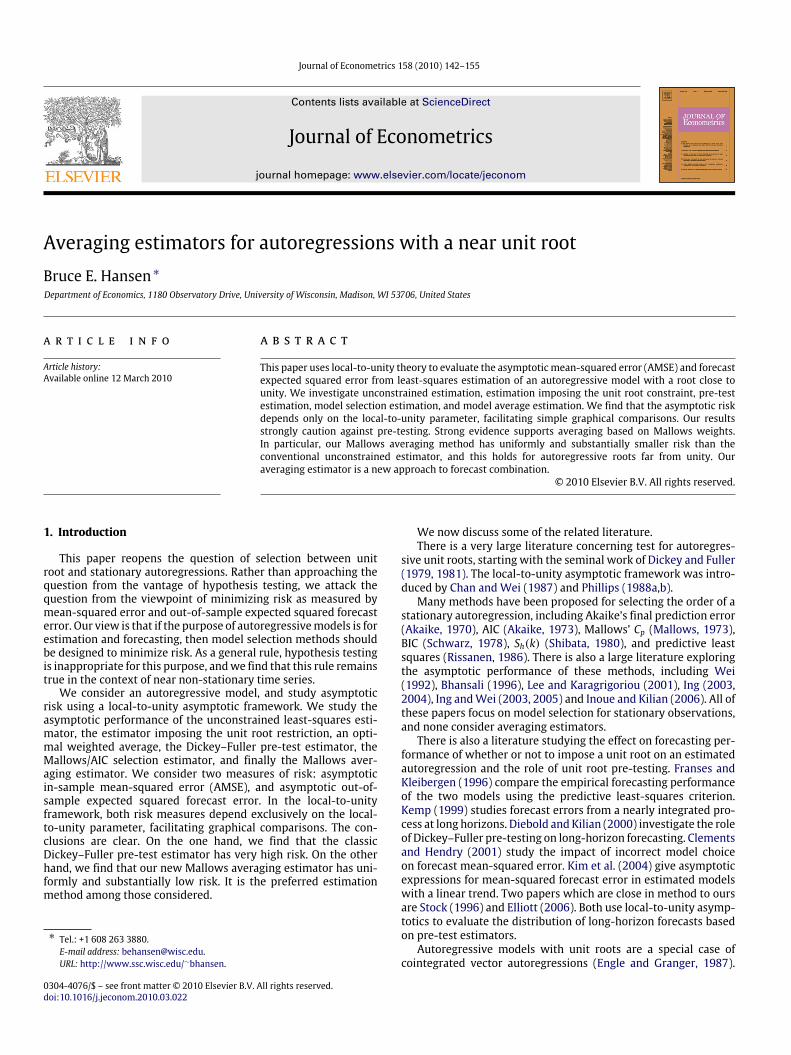
Fig. 1. Asymptotic mean-squared error.

For the averaging estimator, mw(c, p) is a convex weightedaverage of the constrained and unconstrained components, less aninteraction term.While m0(c, p) and m01(c, p) can be calculated analytically, in

general the functionm1(c, p)must be calculated by simulation.The optimal weight wm(c, p) is independent of k and is strictly

between0 and1 for c < 0. Thismeans that theAMSEof the optimalaveraging estimator is strictly less than both the unrestricted andrestricted estimators.The AMSE of the constrained, unconstrained, and optimal

estimators for p = 1 and k = 0 (that is, the functionsm0(c, 1),m1(c, 1) and mwm(c, 1)) are displayed

1 in Fig. 1 for cranging from −20 to 0. This corresponds to the model with afitted intercept and linear time trend (the case with an interceptonly (p = 0) is qualitatively similar). From the display, we cansee that the AMSE of the constrained estimator is approximatelylinear in c , monotonically increasing as c moves away from zero.The AMSE of the unconstrained estimator is also monotonic, butwith the opposite slope. The latter obtains its maximal value of7.3 at c = 0, and asymptotically approaches 3 as c → −∞.The AMSE curves intersect at c = −8.5, meaning that for c >−8.5, the restricted (unit root) estimator has lower AMSE than theunconstrained estimator, while for c < −8.5 the unconstrainedestimator has lower AMSE. For all c , the AMSE of the optimalaveraging estimator is substantially below the AMSE of the othertwo estimators. The optimal estimator is infeasible, but its AMSEsuggests that there are potentially large gains may be availablefrom averaging.

4. Asymptotic forecast risk

In this section we consider an alternative measure of risk, theasymptotic one-step-ahead expected squared forecast error,whichis a more direct measure of forecasting ability than AMSE.

Theorem 2. The asymptotic forecast risk of the constrained estimatoris

f0(c, p, k) ≡ limn→∞

nσ 2E (µn+1 − µn+1)

2= f0(c, p)+ k (18)

where

1 Figs. 1 and 2 are computed on a grid of 101 evenly-spaced points from−20 to 0. Figs. 3–5 are computed on a grid of 21 points. Functions withoutanalytic expressions were calculated by simulation. The asymptotic distributionswere approximated by finite-sample counterparts with 1000 observations. 500,000simulation replications were used.

B.E. Hansen / Journal of Econometrics 158 (2010) 142–155 145

f0(c, p) = ET 20c,

T0c = −cW ∗c (1)+ δ(1)′

(∫ 1

0δδ′)−1 ∫ 1

0δdW . (19)

When p = 0 then T0c = −cWc(1) and

f0(c, 0) = c(exp (2c)− 1

2

).

When p = 1 then T0c = (1− c)Wc(1) and

f0(c, 1) = (1− c)2(exp (2c)− 1

2c

).

The asymptotic forecast risk of the unconstrained estimator is

f1(c, p, k) ≡ limn→∞

nσ 2E(µn+1 − µn+1)2 = f1(c, p)+ k (20)

where

f1(c, p) = E(T 21c)

T1c = δ(1)′(∫ 1

0δδ′)−1 ∫ 1

0δdW

+ X∗c (1)′

(∫ 1

0X∗c X

∗′

c

)−1 ∫ 1

0X∗c dW . (21)

The asymptotic forecast risk of the averaging estimator is

fw(c, p, k) = fw(c, p)w2f1(c, p)+ (1− w)2 f0(c, p)+ 2w (1− w) f01(c, p)+ k (22)

where

fw(c, p) = w2f1(c, p)+ (1− w)2 f0(c, p)+ 2w (1− w) f01(c, p)f01(c, p) = E (T1cT0c) .

The weight which minimizes fw(c, p, k) is

wf (c, p) =f0(c, p)− f01(c, p)

f0(c, p)+ f1(c, p)− 2f01(c, p)

and the minimized risk is

fwf (c, p, k) =f0(c, p)f1(c, p)− f01(c, p)2

f0(c, p)+ f1(c, p)− 2f01(c, p)+ k.

The functions f1(c, p) and f01(c, p) must be calculated bysimulation.The asymptotic forecast risk of the constrained, unconstrained,

and optimal estimators for p = 1 and k = 0 is displayed in Fig. 2.The features are qualitatively similar those displayed in Fig. 1.

5. Pre-testing

The choice between the constrained estimator µt and theunconstrained estimator µt may be determined by the data. Acommon practice is pre-testing using a unit root test. The pre-test estimate selects µt if the test rejects the null of the unitroot, otherwise it selects µt . For concreteness, let us focus on theDickey–Fuller t-test, which is based on the t-ratio

DFn =α − 1s(α)

where s(α) is the OLS standard error for α. Let r be a critical value.(For example, if p = 1 the asymptotic 5% critical value is r =−3.41.) The pre-test estimator is

µdft = µt1 (DFn ≤ r)+ µt1 (DFn > r) .We now present the AMSE and asymptotic forecast risk for this

estimate.

Fig. 2. Asymptotic forecast risk.

Theorem 3.

mdf (c, p, k) = limn→∞

1σ 2

n∑t=1

E(µdft − µt

)2= E (F1c1 (DFc ≤ r))+ E (F0c1 (DFc > r))+ p+ k

and

fdf (c, p, k) = limn→∞

nσ 2E(µdfn+1 − µn+1

)2= E

(T 21c1 (DFc ≤ r)

)+ E

(T 20c1 (DFc > r)

)+ k

where F0c, F1c, T0c , and T1c are defined in (11), (15), (19) and (21),respectively,

DFc =

∫ 10 W

τc dWc(∫ 1

0

(W τc

)2)1/2 ,and

W τc (r) = Wc(r)−

∫ 1

0Wcτ ′

(∫ 1

0ττ ′)−1

τ(r),

τ (r) =

1...rp

.The AMSE and asymptotic forecast risk of the pre-test estimator

are displayed in Figs. 1 and 2, respectively. Both measures of riskare low for small values of−c but quite large for moderate to largevalues of −c . The goal of pre-testing is presumably to gain thebenefits of both the constrained and unconstrained estimators, butexamining the figures we see that this is not the case. The pre-testestimator has smaller risk than the unconstrained estimator onlyfor very small values of −c , but for most of the parameter spacethe pre-test estimator has higher risk, and the discrepancy can bequite large. This is similar to the behavior of pre-test estimates instationary models.This conclusion appears to clash with the assertions in Stock

(1996) and Diebold and Kilian (2000) that pre-testing can be usefulfor selection of forecasting models. However, the tables in Stock(1996) clearly show similar behavior to the results in Figs. 1 and 2,even for his DF-GLS pre-test estimator. Diebold and Kilian (2000)largely miss the difficulty by focusing exclusively on very smalland very large values of |c|—both cases where pre-testing workswell. These papers also focus on the long-horizon forecasting case,where they argue that pre-testing is more valuable, while in thispaper we focus exclusively on one-step-ahead forecasting.

146 B.E. Hansen / Journal of Econometrics 158 (2010) 142–155

6. Mallows selection

As an alternative to pre-testing, the choice between µt and µtcan bemade using an information criterion, such as the AIC, BIC, orMallows. For convenience we focus on the Mallows criterion as itslinear structure is easy to characterize. We discuss selection basedon AIC and BIC following Theorem 5 below.The Mallows (1973) criterion is a penalized sum of squared

errors, designed to be approximately unbiased for the in-sampleAMSE. In our local-to-unitymodel, the optimalMallows criteria forthe unrestricted and restricted models are

M0(c) = nσ 2 + 2σ 2 (m01(c, p)+ k)

and

M1(c) = nσ 2 + 2σ 2 (m1(c, p)+ k) ,

respectively, where σ 2 = n−1∑nt=1

(yt − µt

)2 and σ 2 =n−1

∑nt=1 (yt − µt)

2 are the estimates of σ 2 from the two models.This claim is justified by the following result.

Theorem 4.EM0(c)σ 2

− n→ m0(c, p, k)

EM1(c)σ 2

− n→ m1(c, p, k).

Theorem 4 shows that the criteria M0(c) and M1(c) are (afternormalization) asymptotically unbiased estimates of the AMSE.This demonstrates that these are appropriate Mallows criterionfor model selection. The penalty terms in M0(c) and M1(c) arenon-standard. This is analogous to the finding of Chao and Phillips(1999) in their study of Bayesian model selection in reduced rankVARs.Unfortunately, the criteria M0(c) and M1(c) are infeasible

since they depend on the unknown c. We suggest evaluating thecriterion for the restricted model M0(c) at the restricted valuec = 0, viz.M0 = M0(0) and the criterion for the unrestrictedmodelM1(c) at the opposite asymptote, viz.M1 = limc→−∞M1(c). Sincem01(0, p) = p and limc→−∞m1(c, p) = 2+ p these values are

M0 = nσ 2 + 2σ 2(p+ k)

and

M1 = nσ 2 + 2σ 2(2+ p+ k)

respectively, which are the classic Mallows (1973) criterion forthe restricted and unrestricted models (as p + k is the numberof fitted parameters in the unit root model and 2 + p + k is thenumber of parameters in the unrestricted model). That is, whileM0(c) andM1(c) are optimal yet infeasible, the limitsM0 = M0(0)and M1 = limc→−∞M1(c) correspond to the conventional modelselection criterion.Mallows selection picks the model with the smallest criterion

(M0 or M1). This is equivalent to selecting the unrestrictedestimator when Fn ≥ 2((2+ p+ k)− (p+ k)) = 4 where

Fn = n(σ 2 − σ 2

σ 2

)(23)

is the classic Wald statistic for the joint exclusion of yt−1 and thetime trend from (3). The Mallows selected estimator is then

µmt = µt1 (Fn ≥ 4)+ µt1 (Fn < 4) .

We now characterize the AMSE and asymptotic forecast risk ofMallows selection.

Theorem 5.

mm(c, p, k) = limn→∞

1σ 2

n∑t=1

E(µmt − µt

)2= E (F1c1(Fc ≥ 4))+ E (F0c1 (Fc < 4))+ p+ k

and

fm(c, p, k) = limn→∞

nσ 2E(µmt − µn+1

)2= E(T 21c1(Fc ≥ 4))+ E

(T 20c1(Fc < 4)

)+ k

where F0c, F1c, T0c , and T1c are defined in (11), (15), (19) and (21),and

Fc =(∫ 1

0dWcX∗′c

)(∫ 1

0X∗c X

∗′

c

)−1 (∫ 1

0X∗c dWc

). (24)

From Theorem 5 we can also deduce the asymptotic perfor-mance of AIC and BIC selection. In fact, Mallows and AIC selec-tion are asymptotically equivalent, as AIC selects the unrestrictedestimator when n log

(σ 2/σ 2

)≥ 4, and n log

(σ 2/σ 2

)= Fn +

op(1) in the local-to-unity model. It follows that AIC selection hasthe same asymptotic risk as Mallows selection. In contrast, BICis asymptotically equivalent to restricted estimation, as BIC se-lects the unrestricted estimator when n log

(σ 2/σ 2

)≥ 2 ln(n)

which occurs with probability tending to zero as n diverges, sincen log

(σ 2/σ 2

)≈ Fn has a non-degenerate asymptotic distribution

in the local-to-unity model. Since the unrestricted model is in a lo-cal neighborhood of the restricted model, BIC selects the restrictedmodel with probability approaching one and thus BIC selection hasasymptotic risk equal to the restricted estimator.The AMSE of the Mallows/AIC selection estimator is displayed

in Fig. 1 and its forecast risk is displayed in Fig. 2. (The BIC selectionestimator has the same asymptotic risk as the constrainedestimator.) The risk of the Mallows/AIC selection estimator is veryclose to that of the unconstrained estimator. The evidence suggeststhat there is little reason to consider the selection estimator ratherthan unconstrained estimation.

7. Mallows averaging

Just as for selection, the Mallows criterion for the averagingestimator (Hansen, 2007) is a penalized sum of squared errors,designed to be approximately unbiased for the in-sample AMSE.For anyw let

σ 2(w) = n−1n∑t=1

(yt − µt (w)

)2be the variance estimate using the averaging estimator µt (w). Inthe local-to-unity model the optimal Mallows criterion isMw(c) = nσ 2(w)+ 2σ 2(w (m1(c, p)+ k)

+ (1− w) (m01(c, p)+ k)).This claim is justified by the following result.

Theorem 6.EMw(c)σ 2

− n→ mw(c, p, k).

This shows that the criterion Mw(c) is an asymptoticallyunbiased estimates of the AMSE for the averaging estimator. As inthe case of selection this criterion is unfeasible, and as before wesuggest replacing m1(c, p) with limc→−∞m1(c, p) = 2 + p andm01(c, p)withm01(0, p) = 0, leading to the feasible criterionMw = nσ 2(w)+ 2σ 2 (w(2+ p+ k)+ (1− w) (p+ k))= nσ 2(w)+ 2σ 2 (2w + p+ k)

which is identical to the Mallows averaging criterion proposed inHansen (2007).

B.E. Hansen / Journal of Econometrics 158 (2010) 142–155 147

The Mallows selected weight w is the value which minimizesMw overw ∈ [0, 1]. Since the criterion is quadratic inw there is anexplicit solution.

Theorem 7. The minimizer of Mw is

w =

1−

2Fn

if Fn > 2

0 otherwise

where Fn is the classic Wald statistic (23).

The Mallows averaging estimator is the weighted average ofthe unrestricted and restricted least-squares estimators, using theMallows weight w.µat = wµt +

(1− w

)µt

=

µt if Fn ≤ 2(1−

2Fn

)µt +

(2Fn

)µt otherwise.

Theorem 8. The Mallows selected weight has the asymptotic distri-bution

wd−→ πc =

1−

2Fc

if Fc > 2

0 otherwise,

where Fc is defined in (24). The AMSE of the Mallows averagingestimator is

ma(c) = limn→∞

1σ 2

n∑t=1

E(µat − µt

)2= E

(π2c F1c

)+ E

((1− πc)2 F0c

)− 2cE

(πc (1− πc)

∫ 1

0dWW ∗c

)+ 1

and the asymptotic forecast risk is

fa(c) = limn→∞

nσ 2E(µn+1

(w)− µn+1

)2= E (πcT1c + (1− πc) T0c)2

where F0c, F1c, T0c , and T1c are defined in (11), (15), (19) and (21),respectively.

The AMSE and asymptotic forecast risk of the Mallowsaveraging estimator are displayed in Figs. 1 and 2. Its performanceis stunning relative to the other estimators. In both figures, therisk of the averaging estimator is uniformly smaller than theunrestricted estimator, and for most values of c the improvementis quite significant. The risk reduction (relative to unrestrictiveestimation) is significant even for large values of |c|. For example,at c = −20 the reduction in AMSE is about is about 15%. Overall,the averaging estimator has the impressively low risk, and is thebest choice among the feasible estimators considered.

8. Finite sample MSE and forecast risk

The analysis of the previous sections has been asymptotic. Wehave found that the AMSE and forecast risk are only a function ofthe local-to-unity parameter c and the order of the trend functionp, and is affected by the autoregressive order k only by an interceptshift. In particular, the asymptotic theory is invariant to the othermodel parameters, including those which determine the short-run dynamics. In this section, we investigate whether or not these

features continue to hold in finite samples. For simplicity, we focuson forecast risk, as this is the primary criterion of interest.Our finite sample investigation uses the AR(k+1)model (1)–(2)

with p = 1 and et i.i.d. N(0, 1). We set the trend parametersβ0 = β1 = 0. In this section, we assume that k is known, andconsider the values k = 0, 4, 8. The sample sizes are n = 50 andn = 200.For our first experiment,we set all the remaining autoregressive

parameters to zero, α1 = · · · = αk = 0. This allows us toinvestigate the effects of sample size and autoregressive order,holding the serial correlation properties constant. Setting α0 =c/n, we vary c on a grid from −20 to 0. This implies a range forα0 of [−0.4, 0] for n = 50 and a range of [−0.1, 0] for n = 200.For each parameter configuration, we calculate the forecast risk

nE(µn+1 − µn+1)2 for three estimators: the unrestricted least-

squares estimator µn+1, the Dickey–Fuller pre-test estimator µdfn+1,

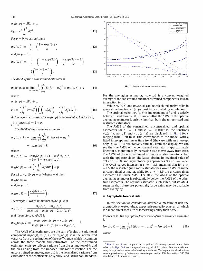
and theMallows averaging estimator µan+1. The riskwas calculatedby Monte Carlo simulation, taking the average of n(µn+1 −µn+1)2across 500,000 simulation draws.The results are presented in Fig. 3. There are six panels, one

for each (n, k) pair. In each panel, the forecast risk is plottedas a function of c. These panels are finite sample analogs of theasymptotic risk as reported in Fig. 2. What is striking is that allof the panels in Fig. 3 are quite similar to Fig. 2. The scaled finitesample forecast risk is nearly identical to the asymptotic risk. Theonly exception can be seen in the lower-left panel, for n = 50and k = 8, where the unrestricted estimator has relatively highforecast risk, and is noticeably dominated by the pre-test andaveraging estimators for all values of c. What is most important,however, is that the risk of the Mallows averaging estimator isuniformly less than that of the unrestricted estimator, in all casesconsidered.Our second experiment adds serial correlation. We do this by

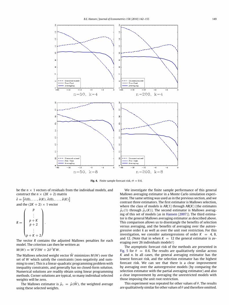
setting the autoregressive parameters as αj = −(−θ)j for j =1, . . . , k, for θ = 0.6 (the results are not sensitive to this choice).We then set α0 = (1 − a1 − · · · ak)c/n as indicated by theasymptotic theory.We repeated the experiment as described above, for k = 4 and

8 (since k = 0 is redundant with the prior experiment). The resultsare presented in Fig. 4 and are very similar to Fig. 3. As predictedby the asymptotic theory, the forecast risk is relatively invariant tothe autoregressive parameters.

9. General Mallows averaging

We now consider a more general setting where the numberof autoregressive lags k is unknown. Let the set of models beindexed by both k and the possible unit root restriction. This ismodel (1)–(2) with k ∈ {0, 1, . . . , K}. For each k = 0, . . . , K , letµt(k) and µt(k) denote the least-squares estimates of µt from theregressions (5) and (6).The averaging estimator is a weighted average of these 2K + 2

estimates. For each k, let w1k be the weight assigned to µt(k),and let w0k be the weight assigned to µt(k). The weights arenon-negative and sum to one: w1k ≥ 0, w0k ≥ 0, and

∑Kk=0

(w0k + w1k) = 1. The general averaging estimator of µt is

µt(W ) =K∑k=0

(w0kµt(k)+ w1kµt(k)

)where

W =

w0k...w0kw1k...w1k

.

148 B.E. Hansen / Journal of Econometrics 158 (2010) 142–155

Fig. 3. Finite sample forecast risk.

The Mallows criterion for weight selection as described byHansen (2007) is

M(W ) =n∑t=1

(yt − µt(W )

)2+ 2σ 2

(K∑k=0

(w0kk+ w1k(2+ k))+ p

)

where

σ 2 =1n

n∑t=1

(yt − µt(K)

)2is the variance estimator from the unrestricted general model.A computationally useful alternative formula for M(W ) is

constructed as follows. Let e(k) = y − µ(k) and e(k) = y − µ(k)

B.E. Hansen / Journal of Econometrics 158 (2010) 142–155 149

Fig. 4. Finite sample forecast risk,Θ = 0.6.

be the n × 1 vectors of residuals from the individual models, andconstruct the n× (2K + 2)matrixe =

[e(0), . . . , e(K), e(0), . . . , e(K)

]and the (2K + 2)× 1 vector

R =

p...

p+ Kp+ 2...

p+ K + 2

.

The vector R contains the adjusted Mallows penalties for eachmodel. The criterion can then be written asM(W ) = W ′e′eW + 2σ 2R′W .

The Mallows selected weight vector W minimizesM(W ) over theset of W which satisfy the constraints (non-negativity and sum-ming to one). This is a linear-quadratic programming problemwithinequality constraints, and generally has no closed-form solution.Numerical solutions are readily obtain using linear programmingmethods. Corner solutions are typical, so many individual selectedweights will be zero.The Mallows estimator is µt = µ(W ), the weighted average

using these selected weights.

We investigate the finite sample performance of this generalMallows averaging estimator in a Monte Carlo simulation experi-ment. The same settingwas used as in the previous section, andwecontrast three estimators. The first estimator is Mallows selection,where the class of models is AR(1) through AR(K ) (the estimatesµt(1) through µt(K)). The second estimator is Mallows averag-ing of this set of models (as in Hansen (2007)). The third estima-tor is the general Mallows averaging estimator as described above.This comparison allows us to disentangle the benefits of selectionversus averaging, and the benefits of averaging over the autore-gressive order k as well as over the unit root restriction. For thisinvestigation, we consider autoregressions of order K = 4, 8,and 12. (Note that in when K = 12 the general estimator is av-eraging over 26 individuals models!)The asymptotic forecast risk of the methods are presented in

Fig. 5 for θ = 0.6. The results are qualitatively similar acrossK and n. In all cases, the general averaging estimator has thelowest forecast risk, and the selection estimator has the highestforecast risk. We can see that there is a clear improvementby averaging over the autoregressive models (by comparing theselection estimator with the partial averaging estimator) and alsoa clear improvement by averaging the unrestricted models withthose imposing the unit root restriction.This experiment was repeated for other values of θ . The results

are qualitatively similar for other values of θ and therefore omitted.

150 B.E. Hansen / Journal of Econometrics 158 (2010) 142–155

Fig. 5. Selection and averaging over k.

10. Conclusion

This paper examined the question of selection and combinationof autoregressive model when the goal is minimizing risk. Usinglocal-to-unity asymptotic methods, we found that two measuresof risk of a variety of estimators are functions only of the local-

to-unity parameter, facilitating direct comparisons. We examinedunconstrained and constrained least-squares estimation, optimalcombination, Dickey–Fuller pre-testing, Mallows selection, andMallows averaging. The numerical comparisons demonstrate thestunning result that the Dickey–Fuller pre-test estimator hasparticularly high risk, while the Mallows averaging estimator has

B.E. Hansen / Journal of Econometrics 158 (2010) 142–155 151

uniformly low risk. We conclude that Mallows averaging is apotentially important forecasting method.Thepaper has confined attention to one-step-ahead forecasting.

It would be useful to use similar methods to study long-horizonforecasting. This presents some special technical challenges and iswell beyond the scope of this paper.Furthermore, the analysis is restricted to univariate autoregres-

sions. A natural extension would be to vector autoregressions,where the question is the number of cointegrating relationships.Based on the analysis in this paper, we expect model averagingmethods will have lower risk than estimation based on cointegra-tion pre-testing. This deserves further study.It is also possible that further improvements can be made by

considering alternative estimators to least squares. Stock (1996)documents that using the efficient unit root tests of Elliott et al.(1996) can reduce the forecast risk of the pre-test estimator. Can-jels and Watson (1997) develop improved methods for estimationof the trend parameters in models with roots local to unity. Thesemethods may be useful in constructing improved forecasts.Finally, as documented by Stock and Watson (2005), simple

rules for forecast combination (assigning each model equalweight) often achieve lower forecast risk than data-dependentcombination methods. This finding suggests that improvementsover the Mallows averaging method may be feasible, and calls forfurther research into improved combination selection.

Acknowledgements

The author’s research was supported by the National ScienceFoundation. The author thanks the guest editors and two refereesfor the helpful comments.

Appendix

The following results will be useful in subsequent calculations.

Lemma 1.

E(Wc(r)2) =exp(2cr)− 1

2c, (25)

E(∫ 1

0W 2c

)=12c

(exp (2c)− 1

2c− 1

), (26)

E (Wc(1)W (1)) =exp(c)− 1

c. (27)

Proof. Using (8) and the fact that dW (s) is an orthogonal process,

E(Wc(r)2)

= E∫ r

0

∫ r

0exp (c (r − s)) exp (c (r − u)) dW (s)dW (u)

=

∫ r

0exp (2c (r − s)) ds

=exp(2cr)− 1

2cwhich is (25). Eq. (26) follows by integration. To show (27),

E (Wc(1)W (1)) = E∫ 1

0

∫ 1

0exp (c (1− s)) dW (s)dW (u)

=

∫ 1

0exp(c(1− s))ds

=exp(c)− 1

c.

Proof of Theorem 1. First, as shown in Lemma1ofHansen (1995),since et is a MDS,

1σ√n

[nr]∑t=1

etd−→ W (r)

anda

σ√nS[nr]

d−→ Wc(r).

Defining the weight matrices D0n = diag{1, n, . . . , np−1} andD1n = diag

{np, n1/2σ/a

}, we have

D−10n δ[nr]d−→ δ(r),

D−11n x[nr]d−→ Xc(r).

Define the orthogonalized series

x∗t = xt − δ′

t

(n∑j=1

δjδ′

j

)−1 n∑j=1

δjxj

z∗t = zt − δ′

t

(n∑j=1

δjδ′

j

)−1 n∑j=1

δjzj

S∗t−1 = St−1 − δ′

t

(n∑j=1

δjδ′

j

)−1 n∑j=1

δjSj−1

and observe thata

σ√nS∗[nr]

d−→ W ∗c (r),

D−11n x∗

[nr]d−→ X∗c (r).

Since the regressions (5) and (6) include δt , the fittedmeans µt andµt are unchanged if we replace xt and zt with x∗t and z

∗t , which we

now assume for the remainder of the Appendix.We now examine the constrained estimator. The regression (6)

has an effective error of can−1St−1 + et . Let

θ∗0 = θ0 −can

(n∑t=1

δtδ′

t

)−1 ( n∑t=1

δtSt−1

)which satisfies

n1/2

σD0n

(θ∗0 − θ0

)=1σD0n

(1n

n∑t=1

δtδ′

t

)−1 (1√n

n∑t=1

δtet

)+ op(1)

d−→

(∫ 1

0δδ′)−1 (∫ 1

0δdW

). (28)

Also

n1/2

σ(α − α) =

(1n

n∑t=1

z∗t z∗′

t

)−1 (1

σ√n

n∑t=1

z∗t et + op(1)

)d−→ Z ∼ N

(0,Q−1

)(29)

where Q = E(z∗t z∗′t

).

We can write

µt − µt = −can−1St−1 +(θ0 − θ0

)′δt + (α − α)

′ z∗t

= −can−1S∗t−1 +(θ∗0 − θ0

)′δt + (α − α)

′ z∗t (30)

152 B.E. Hansen / Journal of Econometrics 158 (2010) 142–155

so

1σ 2

n∑t=1

(µt − µt)2

=c2a2

σ 2n2

n∑t=1

S∗2t−1 +1σ 2

(θ∗0 − θ0

)′ n∑t=1

δtδ′

t

(θ∗0 − θ0

)+1σ 2(α − α)

′

n∑t=1

z∗t z∗′

t (α − α)+ op(1)

d−→ c2

∫ 1

0W ∗2c +

(∫ 1

0dWδ′

)(∫ 1

0δδ′)−1

×

(∫ 1

0δdW

)+ Z ′QZ

= F0c + χ2p + χ2k (31)

where

χ2p =

(∫ 1

0dWδ′

)(∫ 1

0δδ′)−1 (∫ 1

0δdW

)and

χ2k = Z′QZ

are chi-square with degrees of freedom p and k, respectively.Taking expectations of (31) we obtain (10).When p = 0 then there is no δ(r). Thus using (26),

m0(c, 0) = E(c2∫ 1

0W 2c

)= −

c2+exp (2c)− 1

4

which is (12). When p = 1, δ(r) = 1. Thus

m0(c, 1) = E(c2∫ 1

0W ∗2c

)+ 1

= E(c2∫ 1

0W 2c

)− E

(c∫ 1

0Wc

)2+ 1.

Eq. (7) implies

c∫ 1

0Wc = Wc(1)−W (1) (32)

and thus using (25), (26) and (27), we find

m0(c, 1) = E(c2∫ 1

0W 2c

)− EWc(1)2

− EW (1)2 + 2E (Wc(1)W (1))+ 1

= −c2+exp (2c)− 1

4−

(exp (2c)− 1

2c

)+ 2

(exp(c)− 1

c

),

which is (13).We next consider the unconstrained estimator. Note that

µt − µt = δ′

t

(θ0 − θ0

)+ x∗′t

(θ1 − θ1

)+ z∗′t

(α − α

).

We calculate that

n1/2

σD0n

(θ0 − θ0

)d−→

(∫ 1

0δδ′)−1 ∫ 1

0δdW , (33)

n1/2

σD1n

(θ1 − θ1

)d−→

(∫ 1

0X∗c X

∗′

c

)−1 ∫ 1

0X∗c dW , (34)

and

n1/2

σ

(α − α

) d−→ Z (35)

as in (29).We find

1σ 2

n∑t=1

(µt − µt

)2=1σ 2

n∑t=1

(δ′t

(θ0 − θ0

)+ x∗′t

(θ1 − θ1

)+ z∗′t

(α − α

))2

=1σ 2

(θ1 − θ1

)′ n∑t=1

x∗t x∗′

t

(θ1 − θ1

)+1σ 2

(θ0 − θ0

)′ n∑t=1

δtδ′

t

(θ0 − θ0

)+1σ 2

(α − α

)′ n∑t=1

z∗t z∗′

t

(α − α

)+ 2

1σ 2

(θ − θ

)′ n∑t=1

x∗t z∗′

t

(α − α

)d−→

(∫ 1

0dWX∗′c

)(∫ 1

0X∗c X

∗′

c

)−1 (∫ 1

0X∗c dW

)+

(∫ 1

0dWδ′

)(∫ 1

0δδ′)−1 (∫ 1

0δdW

)+ Z ′QZ

= F1c + χ2p + χ2k . (36)

Taking expectations of (36) yields (14).We now examine the averaging estimator. Let θ0(w) = wθ0 +

(1−w)θ∗0 and α(w) = wα+ (1−w)α. We can see that for anyw

n1/2

σD0n

(θ0(w)− θ0

)d−→

(∫ 1

0δδ′)−1 ∫ 1

0δdW

and

n1/2

σ

(α(w)− α

) d−→ Z .

Noting that

µt(w)− µt = wx∗′t(θ1 − θ1

)− (1− w) can−1S∗t−1

+

(θ0(w)− θ0

)′δt +

(α(w)− α

)′ z∗t , (37)

we see

1σ 2

n∑t=1

(µt(w)− µt

)2= w2

1σ 2

(θ1 − θ1

)′ n∑t=1

x∗t x∗′

t

(θ1 − θ1

)+ (1− w)2

c2a2

σ 2n

n∑t=1

S∗2t−1 +1σ 2

(θ0(w)− θ0

)′×

n∑t=1

δtδ′

t

(θ0(w)− θ0

)− 2w (1− w)

canσ 2

×

(θ1 − θ1

)′ n∑t=1

x∗t S∗

t−1 +1σ 2

(α(w)− α

)′×

n∑t=1

z∗t z∗′

t

(α(w)− α

)+ op(1)

B.E. Hansen / Journal of Econometrics 158 (2010) 142–155 153

d−→ w2

(∫ 1

0dWX∗′c

)(∫ 1

0X∗c X

∗′

c

)−1×

(∫ 1

0X∗c dW

)+ (1− w)2 c2

∫ 1

0W ∗2c

− 2w (1− w) c(∫ 1

0dWX∗′c

)(∫ 1

0X∗c X

∗′

c

)−1×

∫ 1

0X∗cW

∗

c + χ2p + χ

2k

= w2F1c + (1− w2)F0c − 2w(1− w)c

×

∫ 1

0dWW ∗c + χ

2p + χ

2k . (38)

Taking expectations establishes (16).To evaluatem01(c, p), note that

m01(c, p) = −Ec∫ 1

0dWWc

+ E

(c∫ 1

0dWδ′

(∫ 1

0δδ′)−1 ∫ 1

0δWc

)+ p

= E

(c∫ 1

0dWδ′

(∫ 1

0δδ′)−1 ∫ 1

0δWc

)+ p (39)

since E∫ 10 dWWc = 0 by the definition of the stochastic integral. It

follows that when p = 0,m01(c, 0) = 0. When p = 1, using (32)and (27),

m01(c, 1) = E(cW (1)

∫ 1

0Wc

)+ 1

= −E(W (1)2

)+ E (W (1)Wc(1))+ 1

=exp(c)− 1

c,

which is (16).The optimalw∗ andmean-squared error are found byminimiz-

ingmw(c, p, k)with respect tow. �

Proof of Theorem 2. First, take the unconstrained estimator. Ob-serve thatµn+1 − µn+1 = δ

′

n+1(θ0 − θ0)+ x∗′

n+1(θ1 − θ1)+ z∗′

n+1(α − α).

Using (33) and (34), note thatn1/2

σ(δ′n+1(θ0 − θ0)+ x

∗′

n+1(θ1 − θ1))

d−→ δ(1)′

(∫ 1

0δδ′)−1 ∫ 1

0δdW + X∗c (1)

′

×

(∫ 1

0X∗c X

∗′

c

)−1 ∫ 1

0X∗c dW = T1c (40)

and thusnσ 2E(δ′n+1(θ0 − θ0)+ x

∗′

n+1(θ1 − θ1))2→ ET 21c .

Furthermore using (35)nσ 2((α − α)(α − α)′)

d−→ ZZ ′,

sonσ 2E((α − α)′z∗n+1)

2=

nσ 2tr E(z∗n+1z

∗′

n+1(α − α)(α − α)′)

→ tr E(z∗n+1z∗′

n+1ZZ′)

= E(Z ′QZ) = k. (41)

Together,

nσ 2E(µn+1 − µn+1)2 =

nσ 2E(δ′n+1(θ0 − θ0)+ x

∗′

n+1(θ1 − θ1))2

+nσ 2E((α − α)z∗n+1z

∗′

n+1(α − α))+ o(1)

→ ET 21c + k

which is (20).Second, take the constrained estimator. We have

µn+1 − µn+1 = −can−1S∗n + (θ∗

0 − θ0)′δn+1 + (α − α)

′z∗n+1.

Using (28),

n1/2

σ(−can−1S∗n + (θ

∗

0 − θ0)′δn+1)

d−→ −cW ∗c (1)+ δ(1)

′

(∫ 1

0δδ′)−1 ∫ 1

0δdW = T0c (42)

and thereforenσ 2E(−can−1S∗n + (θ

∗

0 − θ0)′δn+1)

2→ ET 20c .

As in (41),

nσ 2E((α − α)′z∗n+1)

2→ k.

Thennσ 2E(µn+1 − µn+1)2 =

nσ 2E(−can−1S∗n + (θ

∗

0 − θ0)′δn+1)

2

+nσ 2E((α − α)′z∗n+1)

2+ o(1)

→ ET 20c + k,

which is (18). When p = 0 then T0c = −cWc(1) so f0(c, 0) =c2EWc(1)2 = c(exp(2c)− 1)/2 by (25). When p = 1 then

T0c = −cWc(1)+ c∫ 1

0Wc +W (1) = (1− c)Wc(1)

and therefore f0(c, 1) = (1 − c)2EWc(1)2 = (1 − c)2(exp(2c) −1)/2c.Third, take the averaging estimator. Since

µn+1(w)− µn+1 = w(δ′

n+1(θ0 − θ0)+ x∗′

n+1(θ1 − θ1))+ (1− w)

× (−can−1S∗n + (θ∗

0 − θ0)′δn+1)+ (α(w)− α)

′z∗n+1,

thennσ 2E(µt(w)− µt)2 = w2

nσ 2E(δ′n+1(θ0 − θ0)+ x

∗′

n+1(θ1 − θ1))2

+ (1− w)2nσ 2E(−can−1S∗n + (θ

∗

0 − θ0)′δn+1)

2

+ 2w(1− w)nσ 2E(δ′n+1(θ0 − θ0)

+ x∗′n+1(θ1 − θ1))(−can−1S∗n + (θ

∗

0 − θ0)′δn+1)

+nσ 2E((α(w)− α)z∗n+1z

∗′

n+1(α(w)− α))

+ op(1)d−→ w2ET 21c + (1− w)

2ET 20c+ 2w(1− w)E(T0cT1c)+ k

which is (22).The optimal weight and risk are found byminimizing fw(c, p, k)

with respect tow. �

154 B.E. Hansen / Journal of Econometrics 158 (2010) 142–155

Proof of Theorem 3. From (31) and (36) we have

1σ 2

n∑t=1

(µt − µt)2 d−→ F0c + χ2p + χ

2k

and

1σ 2

n∑t=1

(µt − µt)2 d−→ F1c + χ2p + χ

2k .

By standard calculations we know that DFd−→ DFc . Recalling that

µdf = µt1(DFn ≤ r)+ µt1(DFn > r), we then have

1σ 2

n∑t=1

(µdft − µt)

2=1σ 2

n∑t=1

(µt − µt)21(DFn ≤ r)

+1σ 2

n∑t=1

(µt − µt)21(DFn > r)

d−→ F1c1(DFc ≤ r)+ F0c1(DFc > r)+ χ2p + χ

2k

= F1c1(DFc ≤ r)+ F0c1(DFc > r)+ χ2p + χ2k .

Taking expectations yields the expression formdf (c, p, k).Similarly, using (42) and (40),nσ 2E(µdft − µn+1)

2=nσ 2E[(µn+1 − µn+1)21(DFn ≤ r)]

+nσ 2E[(µn+1 − µn+1)21(DFn > r)]

=nσ 2E[(δ′n+1(θ0 − θ0)+ x

′

n+1(θ − θ))2

× 1(DFn ≤ r)] +nσ 2E[(−can−1S∗n

+ (θ∗0 − θ0)′δn+1)

21(DFn > r)]

+nσ 2E((α − α)z∗n+1z

∗′

n+1(α − α))+ o(1)

→ E[T 21c1(DFc ≤ r)

]+ E[T 20c1(DFc > r)] + k,

which is fdf (c, p, k). �

Proof of Theorem 4. First takeM0(c). Since yt − µt = et − (µt −µt) thenn∑t=1

(yt − µt)2 =n∑t=1

e2t +n∑t=1

(µt − µt)2− 2

n∑t=1

et(µt − µt)

and thus

M0(c)− nσ 2

σ 2=1σ 2

n∑t=1

(e2t − σ2)+

1σ 2

n∑t=1

(µt − µt)2

+2σ 2

σ 2(m01(c, p)+ k)−

2σ 2

n∑t=1

et(µt − µt). (43)

The first three terms have expectations tending to m0(c, p, k) +2(m01(c, p)+ k). The fourth term is−2 times

1σ 2

n∑t=1

et(µt − µt) = −caσ 2n

n∑t=1

etS∗t−1 +1σ 2

n∑t=1

etδ′t(θ∗

0 − θ0)

+1σ 2

n∑t=1

etz∗′t (α − α)

d−→ −c

∫ 1

0dWW ∗c +

∫ 1

0dWδ′

(∫ 1

0δδ′)−1 ∫ 1

0δdW + Z ′QZ

(44)

(using (28)), which has expectation m01(c) + k. Adding thesecomponents, it follows that (43) has expectation tending tom0(c, p, k) as claimed.Next considerM1(c). We have

M1(c)− nσ 2

σ 2=1σ 2

n∑t=1

(e2t − σ2)+

1σ 2

n∑t=1

(µt − µt)2

+2σ 2

σ 2(m1(c, p)+ k)−

2σ 2

n∑t=1

et(µt − µt). (45)

The first three terms have expectation tending to m1(c, p, k) +2(m1(c, p)+ k). The third is−2 times

1σ 2

n∑t=1

et(µt − µt)

=1σ 2

n∑t=1

etx∗′t (θ1 − θ1)+1σ 2

n∑t=1

etz∗′t (α − α)

d−→

∫ 1

0dWX∗c (r)

′

(∫ 1

0X∗c X

∗′

c

)−1 ∫ 1

0X∗c dW

+

∫ 1

0dWδ′

(∫ 1

0δδ′)−1 ∫ 1

0δdW + Z ′QZ (46)

which has expectationm1(c, p)+k. Adding these two components,we see that (45) has expectation tending to m1(c, p, k) asclaimed. �

Proof of Theorem 5. The argument is the same as for Theorem 3,except that we use the fact that Fn

d−→ Fc . �

Proof of Theorem 6. Similar to the argument in the proof ofTheorem 4,

Mw(c)− nσ 2

σ 2=1σ 2

n∑t=1

(e2t − σ2)+

1σ 2

n∑t=1

(µt(w)− µt)2

+2σ 2

σ 2(w(m1(c, p)+ k)+ (1− w)(m01(c, p)+ k))

−w2σ 2

n∑t=1

et(µt − µt)− (1− w)2σ 2

n∑t=1

et(µt − µt).

The first three terms have expectation converging to

mw(c, p, k)+ 2(w(m1(c, p)+ k)+ (1− w)(m01(c, p)+ k)).

The fourth and fifth terms converge to a random variable withexpectation

−2(w(m1(c, p)+ k)+ (1− w)(m01(c, p)+ k))

by (44) and (46). Summing, the entire expression converges to arandom variable with expectationmw(c, p, k), as claimed. �

Proof of Theorem 7. Let et = yt − µt and et = yt − µt . Observethatn∑t=1

(yt − µt(w))2 =n∑t=1

(wet + (1− w)et)2

= w2n∑t=1

e2t + (1− w)2n∑t=1

e2t + 2w(1− w)n∑t=1

et et

= w2n∑t=1

e2t + (1− w)2n∑t=1

e2t + 2w(1− w)n∑t=1

e2t

= nσ 2 + (1− w)2n(σ 2 − σ 2).

B.E. Hansen / Journal of Econometrics 158 (2010) 142–155 155

ThusMwσ 2= n+ (1− w)2Fn + 2(2w + k).

The first-order condition forminimization is 0 = −2(1−w)Fn+4,whose solution is w = 1− 2/Fn. If this value is negative, then theconstrained minimizer is w = 0. �

Proof of Theorem 8. Since Fnd−→ Fc it follows directly that

wd−→ πc . Evaluating Eq. (38) at w = πc and then taking

expectations we obtain the expression from ma(c, p, k). Theargument for fa(c, p, k) is similar. �

References

Akaike, H., 1970. Statistical predictor identification. Annals of the Institute ofStatistical Mathematics 22, 203–419.

Akaike, H., 1973. Maximum likelihood identification of Gaussian autoregressivemoving average models. Biometrika 60, 255–265.

Aznar, Antonio, Salvador, Manuel, 2002. Selecting the rank of the cointegrationspace and the form of the intercept using an information criterion. EconometricTheory 18, 926–947.

Bates, J.M., Granger, C.M.W., 1969. The combination of forecasts. OperationsResearch Quarterly 20, 451–468.

Bhansali, R.J., 1996. Asymptotically efficient autoregressive model selection formultistep prediction. Annals of the Institute of Statistical Mathematics 48,577–602.

Canjels, Eugene, Watson, Mark W., 1997. Estimating deterministic trends in thepresence of serially correlated errors. Review of Economics and Statistics 79,184–200.

Chan, N.H., Wei, Ching-Zong, 1987. Asymptotic inference for nearly nonstationaryAR(1) processes. Annals of Statistics 15, 1050–1063.

Chao, John C., Phillips, Peter C.B., 1999. Model selection in partially nonstationaryvector autoregressive processes with reduced rank structure. Journal ofEconometrics 91, 227–271.

Clemen, R.T., 1989. Combining forecasts: a review and annotated bibliography.International Journal of Forecasting 5, 559–581.

Clements,Michael P., Hendry, David F., 2001. Forecastingwith difference-stationaryand trend-stationary models. Econometrics Journal 4, S1–S19.

Dickey, David A., Fuller, Wayne A., 1979. Distribution of the estimators forautoregressive time series with a unit root. Journal of the American StatisticalAssociation 74, 427–431.

Dickey, David A., Fuller, Wayne A., 1981. Likelihood ratio statistics for autoregres-sive time series with a unit root. Econometrica 49, 1057–1072.

Diebold, Francis X., Kilian, Lutz, 2000. Unit-root tests are useful for selectingforecasting models. Journal of Business and Economic Statistics 18, 265–273.

Diebold, Francis X., Lopez, J.A., 1996. Forecast evaluation and combination.In: Maddala, Rao (Eds.), Handbook of Statistics. Elsevier.

Elliott, Graham, 2006. Unit root pre-testing and forecasting. Working Paper. UCSD.Elliott, Graham, Rothenberg, Thomas J., Stock, James H., 1996. Efficient tests of anautoregressive unit root. Econometrica 64, 813–836.

Engle, Robert F., Granger, Clive W.J., 1987. Co-integration and error correction:representation, estimation and testing. Econometrica 55, 251–276.

Franses, Philip Hans, Kleibergen, Frank, 1996. Unit roots in the Nelson–Plosserdata: do they matter for forecasting? International Journal of Forecasting 12,283–288.

Gonzalo, Jesus, Pitarakis, Jean-Yves, 1998. Specification viamodel selection in vectorerror correction models. Economics Letters 60, 321–328.

Granger, Clive W.J., 1989. Combining forecasts—twenty years later. Journal ofForecasting 8, 167–173.

Granger, Clive W.J., Ramanathan, R., 1984. Improved methods of combiningforecasts. Journal of Forecasting 3, 197–204.

Hansen, Bruce E., 1995. Rethinking the univariate approach to unit root tests: howto use covariates to increase power. Econometric Theory 11, 1148–1171.

Hansen, Bruce E., 2007. Least squares model averaging. Econometrica 75,1175–1189.

Hansen, Bruce E., 2008. Least squares forecast averaging. Journal of Econometrics146, 342–350.

Hansen, Bruce E., 2009. Averaging estimators for regressions with a possiblestructural break. Econometric Theory 35, 1498–1514.

Hansen, Bruce E., Racine, Jeffrey S., 2007. Jackknifemodel averaging.Working Paper.University of Wisconsin.

Hendry, D.F., Clements, M.P., 2002. Pooling of forecasts. Econometrics Journal 5,1–26.

Hjort, Nils Lid, Claeskens, Gerda, 2003. Frequentist model average estimators.Journal of the American Statistical Association 98, 879–899.

Ing, Ching-Kang, 2003.Multistep prediction in autoregressive processes. Economet-ric Theory 19, 254–279.

Ing, Ching-Kang, 2004. Selecting optimal multistep predictors for autoregressiveprocesses of unknown order. Annals of Statistics 32, 693–722.

Ing, Ching-Kang, Wei, Ching-Zong, 2003. On same-realization prediction in aninfinite-order autoregressive process. Journal of Multivariate Analysis 85,130–155.

Ing, Ching-Kang, Wei, Ching-Zong, 2005. Order selection for same-realizationpredictions in autoregressive processes. Annals of Statistics 33, 2423–2474.

Inoue, Atsuhsi, Kilian, Lutz, 2006. On the selection of forecasting models. Journal ofEconometrics 130, 272–306.

Kapetanios, George, 2004. The asymptotic distribution of the cointegration rankestimator under the Akaike information criterion. Econometric Theory 20,735–743.

Kemp, Gordon C.R., 1999. The behavior of forecast errors from a nearly integratedAR(1) model as both sample size and forecast horizon become large.Econometric Theory 15, 238–256.

Kim, Tae-Hwan, Leybourne, Stephen J., Newbold, Paul, 2004. Asymptotic mean-squared forecast errorwhen an autoregressionwith linear trend is fitted to datagenerated by an I(0) or I(1) process. Journal of Time Series Analysis 25, 583–602.

Lee, Sangyeol, Karagrigoriou, Alex, 2001. An asymptotically optimal selection of theorder of a linear process. Sankhya Series A 63, 93–106.

Mallows, C.L., 1973. Some comments on Cp . Technometrics 15, 661–675.Pesaran, M. Hashem, Timmermann, Allan, 2007. Selection of estimation window inthe presence of breaks. Journal of Econometrics 137, 134–161.

Phillips, Peter C.B., 1988a. Regression theory for near-integrated time series.Econometrica 56, 1021–1043.

Phillips, Peter C.B., 1988b. Towards a unified asymptotic theory for autoregression.Biometrika 74, 535–547.

Rissanen, J., 1986. Stochastic complexity and modeling. Annals of Statistics 14,1080–1100.

Schwarz, G., 1978. Estimating the dimension of a model. Annals of Statistics 6,461–464.

Shibata, Ritaei, 1980. Asymptotically efficient selection of the order of themodel forestimating parameters of a linear process. Annals of Statistics 8, 147–164.

Stock, James H., 1996. VAR, error correction and pretest forecasts at long horizons.Oxford Bulletin of Economics and Statistics 58, 685–701.

Stock, J.H., Watson, M.W., 2006. Forecasting with many predictors. In: El-liott, Granger, Timmermann, (Eds.), Handbook of Economic Forecasting. Else-vier, (Chapter 10).

Stock, J.H., Watson, M.W., 1999. A comparison of linear and nonlinear univariatemodels for forecasting macroeconomic time series. In: Engle, , White, (Eds.),Cointegration, Causality and Forecasting: A Festschrift for Clive W.J. Granger.Oxford University Press.

Stock, J.H., Watson, M.W., 2004. Combination forecasts of output growth in a seven-country data set. Journal of Forecasting 23, 405–430.

Stock, J.H.,Watson,M.W., 2005. An empirical comparison ofmethods for forecastingusing many predictors. Working Paper. NBER.

Timmermann, Allan, 2006. Forecast combinations. In: Elliott, Granger, Timmer-mann, (Eds.), Handbook of Economic Forecasting. Elsevier (Chapter 4).

Wei, Ching-Zong, 1992. On predictive least squares principles. Annals of Statistics20, 1–42.