Autonomous Helicopter Aerobatics throughApprenticeship Learning

Pieter Abbeel1, Adam Coates2 and Andrew Y. Ng2

Abstract

Autonomous helicopter flight is widely regarded to be a highly challenging control problem. Despite this fact, human

experts can reliably fly helicopters through a wide range of maneuvers, including aerobatic maneuvers at the edge of

the helicopter’s capabilities. We present apprenticeship learning algorithms, which leverage expert demonstrations to

efficiently learn good controllers for tasks being demonstrated by an expert. These apprenticeship learning algorithms

have enabled us to significantly extend the state of the art in autonomous helicopter aerobatics. Our experimental

results include the first autonomous execution of a wide range of maneuvers, including but not limited to in-place flips,

in-place rolls, loops and hurricanes, and even auto-rotation landings, chaos and tic-tocs, which only exceptional human

pilots can perform. Our results also include complete airshows, which require autonomous transitions between many of

these maneuvers. Our controllers perform as well as, and often even better than, our expert pilot.

Keywords

apprenticeship learning, autonomous flight, autonomous helicopter, helicopter aerobatics, learning from demonstrations

1. Introduction

Autonomous helicopter flight represents a challenging

control problem with high-dimensional, asymmetric, noisy,

non-linear, non-minimum phase dynamics. Helicopters

are widely regarded to be significantly harder to control

than fixed-wing aircraft (see, e.g., Leishman (2000) and

Seddon (1990)) At the same time, helicopters provide

unique capabilities, such as in-place hover and low-speed

flight, important for many applications. The control of

autonomous helicopters thus provides a challenging and

important testbed for learning and control algorithms.

In the ‘‘upright flight regime’’ there has been consider-

able progress in autonomous helicopter flight. For example,

Bagnell and Schneider (2001) achieved sustained autono-

mous hover. Both La Civita et al. (2006) and Ng et al.

(2004b) achieved sustained autonomous hover and accurate

flight in regimes where the helicopter’s orientation is fairly

close to upright. Roberts et al. (2003) and Saripalli et al.

(2003) achieved vision-based autonomous hover and

landing.

In contrast, autonomous flight achievements in other

flight regimes have been limited. Gavrilets et al. (2002a)

achieved a limited set of autonomous aerobatic maneuvers:

a stall-turn, a split-S, and an axial roll. Ng et al. (2004a)

achieved sustained autonomous inverted hover. While

these results significantly expanded the potential capabil-

ities of autonomous helicopters, it has remained difficult

to design control systems capable of performing arbitrary

aerobatic maneuvers at a performance level comparable

to human experts.

This paper brings together various pieces of our work

which have culminated in an algorithm that has enabled

us to rapidly and easily teach our helicopters to fly very

challenging maneuvers through providing expert demon-

strations (Ng et al. 2004a; Abbeel and Ng 2005b,a; Abbeel

et al. 2006a,b, 2007, 2008; Coates et al. 2008). Aside from

bringing together these various pieces of prior work, we

also describe (for the first time) an extension which has

enabled our helicopters to perform a maneuver called

chaos—often considered the most challenging aerobatic

maneuver—by observing an expert demonstrate in-

place flips (rather than observing a chaos). We also provide

details on specifics of our helicopter setup and our state

estimation approach.

1.1. Main Contributions

Our main contributions are: (i) apprenticeship learning algo-

rithms for learning a trajectory-based task specification

from demonstrations; (ii) apprenticeship learning algo-

rithms for modeling the dynamics of the helicopter,

(iii) combining these apprenticeship learning algorithms

1 Department of Electrical Engineering and Computer Sciences,

University of California, Berkeley, Berkeley, CA, USA2 Computer Science Department, Stanford University, Stanford, CA, USA

Corresponding author:

Pieter Abbeel, Department of Electrical Engineering and Computer

Sciences, University of California, Berkeley, Berkeley, CA 94720, USA

Email: pabbeel@cs.berkeley.edu

The International Journal of

Robotics Research

000(00) 1–31

ª The Author(s) 2010

Reprints and permission:

sagepub.co.uk/journalsPermissions.nav

DOI: 10.1177/0278364910371999

ijr.sagepub.com

The International Journal of Robotics Research OnlineFirst, published on June 23, 2010 as doi:10.1177/0278364910371999

with (a variation of) existing optimal control algorithms,

namely, a receding horizon variation of linear quadratic con-

trol methods for non-linear systems (a form of model predic-

tive control) to design autonomous helicopter flight

controllers. This approach has enabled us to teach our heli-

copters new maneuvers in less than an hour. This has enabled

our autonomous helicopters to perform a very wide range of

high-performance aerobatic maneuvers, well beyond the cap-

abilities of any other autonomous helicopter to date.

1.1.1. Apprenticeship Learning for Learning a Task

Specification from Demonstrations. Many tasks in robotics

can be described as a trajectory that the robot should

follow. Unfortunately, specifying the desired trajectory

is often a non-trivial task. For example, when asked to

describe the trajectory that a helicopter should follow

to perform an aerobatic flip, one would have to specify a

trajectory that (i) corresponds to the aerobatic flip task, and

(ii) is consistent with the helicopter’s dynamics. The latter

requires (iii) an accurate helicopter dynamics model for all

of the flight regimes encountered in the vicinity of the tra-

jectory. These coupled tasks are non-trivial for systems

with complex dynamics, such as helicopters. Failing to ade-

quately address these points leads to a significantly more

difficult control problem.

In the apprenticeship learning setting, in which an expert

is available, rather than relying on a hand-engineered target

trajectory, one can instead have the expert demonstrate the

desired trajectory. The expert demonstration yields a

desired trajectory for the robot to follow. Unfortunately,

perfect demonstrations can be hard (if not impossible) to

obtain. However, repeated expert demonstrations are often

suboptimal in different ways, suggesting that a large num-

ber of suboptimal expert demonstrations could implicitly

encode the expert’s intended trajectory.

We propose an algorithm that approximately extracts

this implicitly encoded intended trajectory from multiple

suboptimal expert demonstrations. Properly extracting the

underlying intended trajectory from a set of suboptimal

trajectories requires a significantly more sophisticated

approach than merely averaging the states observed at

each time step. For non-linear systems, a simple arith-

metic average of the trajectories would result in a trajec-

tory that does not obey the constraints of the dynamics

model. Also, in practice, each of the demonstrations will

occur at different rates so that attempting to combine

states from the same time step in each trajectory will not

work properly. We present a generative model that

describes the expert demonstrations as noisy observations

of the unobserved, intended target trajectory, where each

demonstration is possibly warped along the time axis. We

present an expectation–maximization (EM) algorithm—

which uses a (extended) Kalman smoother and an effi-

cient dynamic programming algorithm to perform the

E-step—to both infer the unobserved, intended target tra-

jectory and a time alignment of all of the demonstrations.

Our algorithm allows one to easily incorporate prior

knowledge to further improve the quality of the learned

trajectory.

1.1.2. Learning a Dynamics Model. Helicopter

aerodynamics are, to date, somewhat poorly understood,

and (unlike most fixed-wing aircraft) no textbook models

will accurately predict the dynamics of a helicopter from

only its dimensions and specifications (Seddon 1990;

Leishman 2000). Thus, at least part of the dynamics must

be learned from data.

CIFER1 (Comprehensive Identification from Fre-

quency Responses) is the industry standard for learning

linear models for helicopters (and other rotorcraft) from

data (Tischler and Cauffman 1992; Mettler et al. 1999).

CIFER uses frequency response methods to identify a lin-

ear model. While these linear models have been success-

ful for simulation and control around hover and around

forward flight, they naturally lack the expressiveness to

comprehensively capture non-linear aspects of helicopter

dynamics.

La Civita et al. (2002) proposed a first-principles-based

non-linear model and a frequency domain technique to fit

the unknown parameters from flight data. They also

demonstrated successful control design based upon this

model (La Civita et al. 2003). Gavrilets et al. (2002b) also

proposed a first-principles-based non-linear model and they

fit the unknown parameters based upon a mix of physical

measurements and flight data. They demonstrated success-

ful forward flight, aileron rolls, hammerheads and split-S

maneuvers using controllers designed with this model

(Gavrilets et al. 2002c).

In our work, we also use a mix of first-principles-based

modeling and fitting to flight data. We use a simpler non-

linear model than those used by La Civita et al. (2002) and

Gavrilets et al. (2002b). Our model uses a ‘‘rigid-body’’ state

representation: we model the helicopter’s state by only its

position, velocity, orientation, angular rate, and main rotor

speed. For system identification of the unknown parameters

in the non-linear dynamics model, we optimize the predic-

tion accuracy in the time domain.

While this modeling approach provided good simula-

tion accuracy in flight regimes around level flight, it still

exhibited large prediction errors during simulation of

aggressive aerobatic maneuvers. (We have observed up

to 3g of vertical acceleration error during some maneu-

vers.) While a more complex non-linear model might be

able to address some of the inaccuracies, in our experience

the key limitation was the rigid-body state representation,

which only included the helicopter’s position, orientation,

velocity, angular rate, and main rotor speed. Indeed, the

helicopter generates substantial airflow and the state of the

airflow greatly affects the helicopter dynamics; aside from

that, the helicopter and especially its blades are not exactly

rigid.

These other variables are hard to measure or model.

Higher-order dynamics models provide a well-known

approach to resolve this issue. In the most general setting,

learning non-linear higher-order models from data pre-

sents many challenging issues which include: the choice

of the order of the model, handling potential data sparsity

in certain flight regimes, the potential presence of unob-

servable or uncontrollable modes and their stability.

2 The International Journal of Robotics Research 00(000)

Within the scope of this paper, we do not address these

issues. We restrict ourselves to describing a relatively

simple solution applicable to the setting of having a heli-

copter fly particular maneuvers. Our approach uses time-

aligned trajectories—obtained when extracting the task/

trajectory description from multiple demonstrations—to

learn local corrections to the baseline non-linear model.

Our experiments show that the resulting models are suffi-

ciently accurate to develop controllers for highly aggres-

sive aerobatic maneuvers.

1.1.3. Autonomous Helicopter Flight. We present the first

successful autonomous completion of the following

maneuvers: continuous in-place flips and rolls, a continu-

ous tail-down ‘‘tic-toc’’, loops, loops with pirouettes,

stall-turns with pirouette, ‘‘hurricane’’ (fast backward

funnel), knife-edge, immelmann, slapper, sideways tic-

toc, traveling flips, inverted tail-slide, and even auto-

rotation landings and chaos. Not only are our autonomous

helicopters the first to complete such maneuvers autono-

mously, our helicopters are also able to continuously repeat

the maneuvers without any pauses in between. Thus, the

controller has to provide continuous feedback during the

maneuvers, and cannot, for example, use a period of hover-

ing to correct errors from the first execution of the maneu-

ver before performing the maneuver a second time. In fact,

we also have our helicopter fly complete aerobatic air-

shows, during which our helicopter executes a wide variety

of aerobatic maneuvers in rapid sequence.

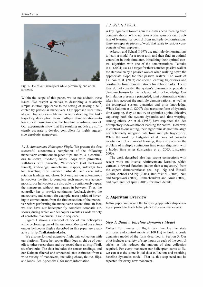
Figure 1 shows a snapshot of one of our helicopters

while performing one of the airshows. Movies of our auton-

omous helicopter flights described in this paper are avail-

able at http://heli.stanford.edu.

We also performed extensive flight data collection with

our platform. These helicopter flight logs might be of ben-

efit to other researchers and we posted them at http://heli.

stanford.edu. The data includes the sensor readings, and

our Kalman filtered and smoothed state estimates from a

wide variety of maneuvers, including chaos, tic-toc, flips,

and loops. See Appendix C for more information.

1.2. Related Work

A key ingredient towards our results has been learning from

demonstrations. While no prior works span our entire set-

ting of learning for control from multiple demonstrations,

there are separate pieces of work that relate to various com-

ponents of our approach.

Atkeson and Schaal (1997) use multiple demonstrations

to learn a model for a robot arm, and then find an optimal

controller in their simulator, initializing their optimal con-

trol algorithm with one of the demonstrations. Tedrake

et al. (2004) use as a target for their actuated passive walker

the steps taken by a passive walker when walking down the

appropriate slope for that passive walker. The work of

Calinon et al. (2007) considered learning trajectories and

constraints from demonstrations for robotic tasks. There,

they do not consider the system’s dynamics or provide a

clear mechanism for the inclusion of prior knowledge. Our

formulation presents a principled, joint optimization which

takes into account the multiple demonstrations, as well as

the (complex) system dynamics and prior knowledge.

While Calinon et al. (2007) also use some form of dynamic

time warping, they do not try to optimize a joint objective

capturing both the system dynamics and time-warping.

Among others, An et al. (1988) have exploited the idea

of trajectory-indexed model learning for control. However,

in contrast to our setting, their algorithms do not time align

nor coherently integrate data from multiple trajectories.

While the work by Listgarten et al. does not consider

robotic control and model learning, they also consider the

problem of multiple continuous time series alignment with

a hidden time series (Listgarten et al. 2005; Listgarten

2006).

The work described also has strong connections with

recent work on inverse reinforcement learning, which

extracts a reward function (rather than a trajectory) from

the expert demonstrations; see, e.g., Ng and Russell

(2000), Abbeel and Ng (2004), Ratliff et al. (2006), Neu

and Szepesvari (2007), Ramachandran and Amir (2007),

and Syed and Schapire (2008), for more details.

2. Algorithm Overview

In this paper, we present the following apprenticeship learn-

ing approach to teach helicopters to fly new maneuvers:

Step 1. Build a Baseline Dynamics Model

Collect 20 minutes of flight data (we log the state

estimates and control inputs at 100 Hz) to build a crude

dynamics model of the form described in Section 3. Our

pilot includes a variety of step inputs on each of the control

sticks, as this reduces the amount of data collection

required. For every maneuver our helicopter learns to fly,

we can use the same initial data collection and resulting

baseline dynamics model. That is, this step need not be

repeated for every new maneuver.

Fig. 1. One of our helicopters while performing one of the

airshows.

Abbeel et al. 3

Step 2. Apprenticeship Learning for Target

Trajectory and Refined Dynamics Model

(a) Collect about 10 demonstrations of the desired maneu-

ver or airshow from our expert pilot. Typically about five of

the demonstrations are reasonably high performance, and

we choose these and feed them (together with the crude

dynamics model from Step 1) into our trajectory learning

algorithm described in Section 4, which provides us with

a target trajectory.

(b) We use the demonstrations of the desired maneuvers

to learn a high-accuracy dynamics model which is specific

to the part of the flight envelope encountered when flying

the desired maneuver. As will become clear, we leverage

the output of our trajectory learning algorithm (Step 1) to

learn this higher accuracy model. (See Section 5.)

Step 3. Autonomous Flight Control

(a) Choose a reward function that penalizes for deviation

from the inferred target trajectory. In our experiments we

found there is a fairly wide range of reward functions that

work well—likely because the inferred target trajectory is

very close to a trajectory the helicopter could fly. This was

often not the case when attempting to use hand-specified

target trajectories.

(b) Run a standard generalization of the linear quadratic

regulator (LQR) for non-linear systems (off-line) to find

a sequence of quadratic cost-to-go functions for each time.

The cost-to-go function for time t is an estimate of the

expected sum of costs accumulated from time t until the

end of the trajectory when executing an optimal controller

from then on. (See Section 6.)

(c) Fly our helicopter autonomously: we run a receding hor-

izon version of the off-line LQR-based controller, which

uses the cost-to-go functions for each time step from the

off-line run as its final cost for each receding horizon

computation.

(d) If flight performance is satisfactory, we are done. Other-

wise, incorporate the data from the autonomous flight to

learn an improved dynamics model. Then go to Step 3(b).

3. Helicopter Dynamics Model

We describe a fairly simple non-linear helicopter model

and our parameter learning (system identification) algo-

rithm for this model. This model has been sufficiently accu-

rate to perform autonomous hover, low-speed flight and

funnels. In Section 5 we describe a more expressive exten-

sion: the extension has the same model structure, however,

the parameters will then become ‘‘local’’ rather than global.

This will enable it to capture helicopter dynamics suffi-

ciently well for control design for aggressive aerobatic

maneuvers.

3.1. Helicopter State and Inputs

The helicopter state comprises its position, orientation,

velocity, and angular velocity. The helicopter is controlled

via a four-dimensional action space:

1. u1 and u2: The latitudinal (left—right) and longitudinal

(front—back) cyclic pitch controls. They are also often

called elevator and aileron. They change the pitch

angle of the main rotor throughout each cycle and can

thereby cause the helicopter to pitch forward/backward

or to roll left/right. By pitching and rolling the helicop-

ter, the pilot can affect the direction of the main thrust,

and hence the direction in which the helicopter

moves.1

2. u3: The yaw rate input commands a reference yaw rate

(rotation rate of the helicopter about its vertical axis) to

an on-board control system. The on-board control sys-

tem runs a PID controller which controls the tail rotor

pitch angle, which in turn changes the tail rotor thrust,

which in turn—as the tail rotor is offset from the center

of gravity (CG) of the helicopter—results in control-

ling the rotation of the helicopter about its vertical axis.

The on-board control system uses a Futaba gyro to

sense the helicopter’s yaw rate.

3. u4: The main rotor collective pitch control changes the

pitch angle of the main rotor’s blades by rotating the

blades around an axis that runs along the length of the

blade. The resulting amount of upward thrust (gener-

ally) increases with this pitch angle; thus, this control

affects the main rotor’s thrust.

By using the cyclic pitch and tail rotor controls, the pilot

can rotate the helicopter into any orientation. This enables

the pilot to direct the thrust of the main rotor in any partic-

ular direction and thus fly in any particular direction.

3.2. Model Structure

We learn a model from flight data that predicts linear and

angular accelerations as a function of the current state and

inputs. Accelerations are then integrated to obtain veloci-

ties, angular rates, position and orientation over time. As

is standard, to take advantage of symmetries of the helicop-

ter, we model the linear and angular accelerations in a

‘‘body-coordinate’’ frame attached to the helicopter. In this

body-coordinate frame, the x-axis always points forward,

the y-axis always points to the right, and z-axis always

points down with respect to the helicopter.

In particular, we use the following model for the linear

and angular accelerations as a function of current state and

control inputs:

_u ¼ vr � wqþ Axuþ gx þ wu;_v ¼ wp� ur þ Ayvþ gy þ D0 þ wv;_w¼ uq� vpþ Azwþ gz þ C4u4 þ D4 þ ww;_p ¼ qrðIyy � IzzÞ=Ixx þ Bxpþ C1u1 þ D1 þ wp;_q ¼ prðIzz � IxxÞ=Iyy þ Byqþ C2u2 þ D2 þ wq;_r ¼ pqðIxx � IyyÞ=Izz þ Bzr þ C3u3 þ D3 þ wr:

ð1Þ

Here ðu; v;wÞ, ðp; q; rÞ, and ðgx; gy; gzÞ denote the linear

velocities, the angular rates, and gravity expressed in a

frame attached to the helicopter. As the velocities are

expressed in the helicopter frame, they can change even

when no forces are exerted on the helicopter when the heli-

copter is rotating. This is captured by the terms vr � wq,

4 The International Journal of Robotics Research 00(000)

wp� ur, and uq� vp. Similarly, if the moments of inertia

are different for different main axes, the angular rates can

change without any moments being exerted on the helicop-

ter. This is captured by the inertial coupling terms

qrðIyy � IzzÞ=Ixx, prðIzz � IxxÞ=Iyy, and pqðIxx � IyyÞ=Izz.

The remaining terms model the forces and moments being

exerted on the helicopter. Our particular choice of model is

relatively simple and has a sparse dependence on the cur-

rent velocities, angular rates, and inputs. The terms wu,

wv, ww, wp, wq, and wr are zero mean Gaussian random

variables, which represent the perturbance of the accelera-

tions due to noise (or unmodeled effects). The coefficients

A;B;C;D are determined from flight data.

During powered flight the governor closes an on-board

feedback loop which tries to keep the engine, and hence the

main rotor, at a fixed speed. However, during auto-rotation,

the main rotor is driven by airflow through the blades.

Hence, for auto-rotation we include the main rotor speed

into the helicopter state representation. See Appendix B for

details.

Our model makes several simplifying assumptions.

It does not incorporate the dynamics of the airflow around

the helicopter. It assumes the four control inputs each only

affect one of the axes, moreover it assumes their effects are

linear and independent of the current state. This is known

not to be true. There is some coupling between the control

inputs. The amount of air-intake depends on the state of the

helicopter and directly influences the effectiveness of the

control inputs. A concrete example thereof is the transla-

tional lift phenomenon: for a given (positive) collective

pitch angle, flying forward generates additional (upward)

lift compared with when hovering. It also assumes that drag

forces are linear in the velocity, whereas most physics mod-

els suggest they are quadratic. The model assumes the

obtained angular rates reach a steady-state value for a given

control input according to a first-order differential equa-

tion. For the roll and pitch axes, this ignores the blade flap-

ping effects and the dynamics of the servos used to exert the

cyclic control inputs. For the yaw axis, it does not explicitly

model the dynamics of the single-axis control loop on

board the helicopter which uses sensor feedback from a

gyro to control the yaw rate. Neither does it model the

dynamics of the servo driving the tail rotor pitch angle

inside this single-axis control loop. In the model we used

for our experiments, we ignored the inertial coupling terms.

Extensive experimentation with incorporating the inertial

coupling showed no improvements in simulation accuracy.

This might indicate that for our helicopters the rotational

inertia of the helicopter is dominated by the fast spinning

rotor—rather than by the mass distribution of the

helicopter.

Despite the various simplifications, this model has

enabled us to design high-performance flight controllers for

our helicopters in stationary flight regimes, including

hover, inverted hover, forward flight, and funnels

(Ng et al. 2004a; Abbeel et al. 2007). For non-stationary

flight regimes, modifications to the dynamics model were

necessary, as described in Section 5.

3.3. Parameter Learning/Identification

To learn the coefficients, we record data from our expert

pilot flying the helicopter through the flight regimes we

would like to model.

In the dynamics model of Equations (1) the unknowns

appear linearly, and they could readily be estimated from

(state, control input) data logs using linear regression,

which would give the least-squares estimate. However,

we need not necessarily use the least-squares criterion. For

example CIFER1 (Tischler and Cauffman 1992; Mettler

et al. 1999) finds the parameters that minimize a frequency

domain error criterion. This allows it to penalize less for fit-

ting errors in regions of the frequency domain where it esti-

mates there to be more noise.

CIFER1 is accepted to be the state of the art in estimat-

ing linear models from helicopter flight data. Being a fre-

quency domain method, however, CIFER1 only applies

to linear models. We have proposed a method which per-

forms as well as CIFER1 when learning linear models for

our helicopters, and which does allow application to the

non-linear setting (Abbeel et al. 2006a). This method opti-

mizes the simulation accuracy of the resulting model over

time intervals of several seconds. While more efficient

methods are sometimes applicable, for a sufficiently small

set of parameters (as in our model), we can simply perform

gradient-based numerical optimization to find the para-

meters which optimize the open-loop simulation accuracy

as evaluated over several seconds long intervals of flight

data. Inspecting the results, optimizing the simulation accu-

racy criterion typically results in a model with larger coef-

ficients compared with learning with the least-squares

criterion. While the simulation accuracy criterion models

have led to better control performance in some experi-

ments, we have found that models obtained with least

squares have often also been sufficiently accurate for

control.

4. Learning a Reward Function from Multiple

Demonstrations

For robots with complex dynamics, such as helicopters, it

can be very challenging to hand-engineer a good target tra-

jectory. We consider the apprenticeship learning setting, in

which an expert is available. Hence, rather than relying on a

hand-engineered target trajectory, we can instead have the

expert demonstrate the desired trajectory. In this section we

describe our probabilistic approach for inferring an expert’s

intended trajectory from a set of demonstrations.

4.1. Generative Model

4.1.1. Basic Generative Model. We are given M demonstra-

tion trajectories of length Nk , for k ¼ 0; . . . ;M � 1. Each

trajectory is a sequence of states, skj , and control inputs,

ukj , composed into a single state vector:

Abbeel et al. 5

ykj ¼

skj

ukj

" #; for j ¼ 0; . . . ;Nk � 1; k ¼ 0; . . . ;M � 1:

Our goal is to estimate a ‘‘hidden’’ intended target trajec-

tory of length T , denoted similarly:

zt ¼s?tu?t

� �; for t ¼ 0; . . . ; T � 1:

We use the following notation: y ¼ fykj jj ¼ 0;. . . ;

Nk � 1; k ¼ 0; . . . ; M � 1g, z ¼ fzt j t ¼ 0; . . . ; T � 1g,and similarly for other indexed variables.

The generative model for the intended trajectory is

given by an initial state distribution z0 � Nðm0;S0Þ and

an approximate model of the dynamics

ztþ1 ¼ f ðztÞ þ oðzÞt ; oðzÞt � Nð0;SðzÞÞ: ð2Þ

The dynamics model does not need to be particularly accu-

rate: in our experiments, we use a single generic model

learned from a large corpus of data that is not specific to

the trajectory we want to perform. In our experiments

(Section 9) we provide some concrete examples showing

how accurately the generic model captures the true

dynamics for our helicopter.2

Our generative model represents each demonstration as

a set of independent ‘‘observations’’ of the hidden, intended

trajectory z. Specifically, our model assumes

ykj ¼ ztk

jþ oðyÞj ; oðyÞj � Nð0;SðyÞÞ: ð3Þ

Here tkj is the time index in the hidden trajectory to which

the observation ykj is mapped. The noise term in the obser-

vation equation captures both inaccuracy in estimating the

observed trajectories from sensor data, as well as errors in

the maneuver that are the result of the human pilot’s imper-

fect demonstration.3

The time indices τkj are unobserved, and our model

assumes the following distribution with parameters dki :

Pðtkjþ1 j τk

j Þ ¼

dk1 if τk

jþ1 � τkj ¼ 1

dk2 if τk

jþ1 � τkj ¼ 2

dk3 if τk

jþ1 � τkj ¼ 3

0 otherwise

8>><>>: ; ð4Þ

tk0 � 0: ð5Þ

To accommodate small, gradual shifts in time between the

hidden and observed trajectories, our model assumes the

observed trajectories are subsampled versions of the hidden

trajectory. We found that having a hidden trajectory length

equal to twice the average length of the demonstrations, i.e.

T ¼ 21

M

XMk¼1

Nk

!;

gives sufficient resolution.

Figure 2 depicts the graphical model corresponding to

our basic generative model. Note that each observation ykj

depends on the hidden trajectory’s state at time tkj , which

means that for tkj unobserved, yk

j depends on all states in the

hidden trajectory which it could be associated with.

4.1.2. Extensions to the Generative Model. Thus far we

have assumed that the expert demonstrations are misa-

ligned copies of the intended trajectory merely corrupted

by Gaussian noise. Listgarten et al. have used this same

basic generative model (for the case where f ð�Þ is the iden-

tity function) to align speech signals and biological data

(Listgarten et al. 2005; Listgarten 2006). We now augment

the basic model to account for other sources of error which

are important for modeling and control.

Learning Local Model Parameters. For many systems,

we can substantially improve our modeling accuracy by

using a time-varying model ftð�Þ that is specific to the vici-

nity of the intended trajectory at each time t. We express ftas our ‘‘crude’’ model, f , augmented with a bias term4, b?t :

ztþ1 ¼ ftðztÞ þ oðzÞt � f ðztÞ þ b?t þ oðzÞt :

To regularize our model, we assume that b?t changes only

slowly over time. We have b?tþ1 � Nðb?t ;SðbÞÞ.We incorporate the bias into our observation model by

computing the observed bias bkj ¼ yk

j � f ðykj�1Þ for each

of the observed state transitions, and modeling this as a

direct observation of the ‘‘true’’ model bias corrupted by

Gaussian noise. The result of this modification is that the

intended trajectory must not only look similar to the

demonstration trajectories, but it must also obey a

Fig. 2. Graphical model representing our trajectory assumptions.

(Shaded nodes are observed.)

Fig. 3. Example of graphical model when t is known. (Shaded

nodes are observed.)

6 The International Journal of Robotics Research 00(000)

dynamics model which includes those errors consistently

observed in the demonstrations.

Factoring out Demonstration Drift. It is often difficult,

even for an expert pilot, during aerobatic maneuvers to

keep the helicopter centered around a fixed position. The

recorded position trajectory will often drift around uninten-

tionally. Since these position errors are highly correlated,

they are not explained well by the Gaussian noise term in

our observation model.

To capture such slow drift in the demonstrated trajec-

tories, we augment the latent trajectory’s state with a

‘‘drift’’ vector dkt for each time t and each demonstrated tra-

jectory k. We model the drift as a zero-mean random walk

with (relatively) small variance. The state observations are

now noisy measurements of zt þ dkt rather than merely zt.

Incorporating Prior Knowledge. Even though it might

be hard to specify the complete intended trajectory in state

space, we might still have prior knowledge about the trajec-

tory. Hence, we introduce additional observations rt ¼rðztÞ corresponding to our prior knowledge about the

intended trajectory at time t. The function rðztÞ computes

some features of the hidden state zt and our expert supplies

the value rt that this feature should take. For example, for

the case of a helicopter performing an in-place flip, we use

an observation that corresponds to our expert pilot’s knowl-

edge that the helicopter should stay at a fixed position while

it is flipping. We assume that these observations may be cor-

rupted by Gaussian noise, where the variance of the noise

expresses our confidence in the accuracy of the expert’s

advice. In the case of the flip, the variance expresses our

knowledge that it is, in fact, impossible to flip perfectly in-

place and that the actual position of the helicopter may vary

slightly from the position given by the expert.

Incorporating prior knowledge of this kind can greatly

enhance the learned intended trajectory. We give more

detailed examples in Section 9.

4.1.3. Model Summary. In summary, we have the following

generative model:

ztþ1 ¼ f ðztÞ þ b?t þ oðzÞt ; ð6Þ

b?tþ1 ¼ b?t þ oðbÞt ; ð7Þ

dktþ1 ¼ dk

t þ oðdÞt ; ð8Þ

rt ¼ rðztÞ þ oðrÞt ; ð9Þ

ykj ¼ ztk

jþ dk

j þ oðyÞj ; ð10Þ

tkj � Pðτk

jþ1jτkj Þ: ð11Þ

Here oðzÞt ;oðbÞt ;o

ðdÞt ;oðrÞt ;o

ðyÞj are zero-mean Gaussian ran-

dom variables with respective covariance matrices

SðzÞ;SðbÞ;SðdÞ;SðrÞ;SðyÞ. The transition probabilities for τkj

are defined by Equations (4) and (5) with parameters

dk1 ; d

k2 ; d

k3 (collectively denoted by d).

4.2. Trajectory Learning Algorithm

Our learning algorithm automatically finds the time-

alignment indexes τ, the time-index transition probabilities

d, and the covariance matrices Sð�Þ by (approximately)

maximizing the joint likelihood of the observed trajectories

y and the observed prior knowledge about the intended tra-

jectory ρ, while marginalizing out over the unobserved,

intended trajectory z. Concretely, our algorithm (approxi-

mately) solves

maxτ;Sð�Þ;d logPðy; ρ; τ ; Sð�Þ; dÞ: ð12Þ

Then, once our algorithm has found τ; d;Sð�Þ, it finds

the most likely hidden trajectory, namely the trajectory z

that maximizes the joint likelihood of the observed trajec-

tories y and the observed prior knowledge about the

intended trajectory ρ for the learned parameters.5 τ; d;Sð�Þ.The joint optimization in Equation (12) is difficult

because (as can be seen in Figure 2) the lack of knowl-

edge of the time-alignment index variables τ introduces a

very large set of dependencies between all of the variables.

However, when τ is known, the optimization problem in

Equation (12) greatly simplifies thanks to context

specific independencies (Boutilier et al. 1996). When τ is

fixed, we obtain a model such as that shown in Figure 3.

In this model we can directly estimate the multinomial

parameters d in closed form; and we have a standard

hidden Markov model (HMM) parameter learning problem

for the covariances Sð�Þ, which can be solved using the

EM algorithm (Dempster et al. 1977), often referred to

as Baum—Welch in the context of HMMs. Concretely,

for our setting, the EM algorithm’s E-step computes

the pairwise marginals over sequential hidden state

variables by running a (extended) Kalman smoother;

the M-step then uses these marginals to update the covar-

iances Sð�Þ.To also optimize over the time-indexing variables τ,

we propose an alternating optimization procedure. For

fixed Sð�Þ and d, and for fixed z, we can find the optimal

time-indexing variables τ using dynamic programming

over the time-index assignments for each demonstration

independently. The dynamic programming algorithm to

find t is known in the speech recognition literature as

dynamic time warping (Sakoe and Chiba 1990) and in

the ?A3B2 tlsb -.014w?> biological sequence alignment

literature as the Needleman–Wunsch algorithm Needleman

and Wunsch(1970). The fixed z we use is the one that max-

imizes the likelihood of the observations for the current set-

ting of parameters τ; d;Sð�Þ. Fixing z means the dynamic

time-warping step only approximately optimizes the origi-

nal objective and we have no guarantees that it will opti-

mize the original objective. Unfortunately, without fixing

z, the independencies required to obtain an efficient

dynamic programming algorithm do not hold. In our

experiments the approximation of fixing z when optimizing

over τ has worked very well.6

Abbeel et al. 7

In practice, rather than alternating between complete

optimizations over Sð�Þ; d and τ, we only partially optimize

over Sð�Þ, running only one iteration of the EM algorithm.

We provide the complete details of our algorithm in

Appendix A.

5. Improved Helicopter Dynamics Model by

Local Parameter Learning

For complex dynamical systems, the state zt used in the

dynamics model often does not correspond to the ‘‘com-

plete state’’ of the system, since the latter could involve

large numbers of previous states or unobserved variables

that make modeling difficult. This is particularly true for

helicopters. The state of the helicopter is only very crudely

captured by the 12-dimensional rigid-body state represen-

tation we use for our controllers. The ‘‘true’’ physical state

of the system includes, among others, the airflow around

the helicopter, the rotor head speed, and the actuator

dynamics.

To construct an accurate non-linear model to predict

ztþ1 from zt, using the aligned data, one could use locally

weighted linear regression (Atkeson et al. 1997), where a

linear model is learned based on a weighted dataset. Data

points from our demonstrations that have a history similar

to the current state, zt, would be weighted more highly than

data far away. While this allows us to build a more accurate

model, the weighted regression must be done online, since

the weights depend on the current state and its history. For

performance reasons7 this may often be impractical.

However, as we only seek to model the system

dynamics along a specific trajectory, knowledge of both

zt and how far we are along the trajectory is often sufficient

to accurately predict the next state ztþ1. Thus, we weight

data only based on the time index, and learn a parametric

model in the remaining variables (which, in our experi-

ments, has the same form as the global ‘‘crude’’ model,

f ð�Þ). Concretely, when estimating the model for the

dynamics at time t, we weight a data point at time t0 by8

W ðt0Þ ¼ exp �ðt � t0Þ2

s2

!;

where s is a bandwidth parameter. Typical values for s are

between 1 and 2 s in our experiments. Since the weights for

the data points now only depend on the time index, we can

precompute all models ftð�Þ along the entire trajectory. The

ability to precompute the models is a feature crucial to our

control algorithm, which relies heavily on fast simulation.

Once the alignments between the demonstrations are

computed by our trajectory learning algorithm, we can use

the time-aligned demonstration data to learn a sequence of

trajectory-specific models. The time indices of the aligned

demonstrations now accurately associate the demonstration

data points with locations along the learned trajectory,

allowing us to build models for the state at time t using the

appropriate corresponding data from the demonstration

trajectories.9

6. Optimal Control

6.1. Linear Quadratic Methods

LQR control problems form a special class of optimal con-

trol problems, for which the optimal policy can be com-

puted efficiently. In LQR the set of states is given by

S ¼ Rn, the set of actions/inputs is given by A ¼ Rp, and

the dynamics model is given by

stþ1 ¼ Atst þ Btut þ wt;

where for all t ¼ 0; . . . ;H we have that

At 2 Rn�n;Bt 2 Rn�p and wt is a zero-mean random vari-

able (with finite variance). The reward for being in state

st and taking action/input ut is given by

�sTt Qtst � uT

t Rtut:

Here Qt;Rt are positive semi-definite matrices which para-

meterize the reward function. It is well known that the opti-

mal policy for the LQR control problem is a time-varying

linear feedback controller which can be efficiently com-

puted using dynamic programming. Although the standard

formulation presented above assumes the all-zeros state is

the most desirable state, the formalism is easily extended

to the task of tracking a desired trajectory s�0; . . . ; s�H .

The standard extension (which we use) expresses the

dynamics and reward function as a function of the error

state et ¼ st � s�t rather than the actual state st. (See, e.g.,

Anderson and Moore (1989) for more details on linear

quadratic methods.)

This approach is commonly extended to non-linear sys-

tems by simply iterating the following two steps:

1. Compute a linear approximation to the dynamics and a

quadratic approximation to the reward function around

the trajectory obtained when using the current policy.

2. Compute the optimal policy for the LQR problem

obtained in Step 1 and set the current policy equal to

the optimal policy for the LQR problem.

In our experiments, we have a quadratic reward function,

thus the only approximation made in the first step is the lin-

earization of the dynamics. To bootstrap the process, we

linearize around the target trajectory in the first iteration.

This approach has been called Gauss–Newton LQR,

iterative LQR (iLQR) and differential dynamic program-

ming (DDP). Technically, DDP (Jacobson and Mayne

1970) is a slightly different algorithm which also includes

one additional higher-order term in the approximation. DDP

is readily derived by writing out a second-order expansion of

the Bellman back-up equations.10 We use the name Gauss–

Newton LQR or even abbreviate it as just LQR.

With appropriate step sizing, Gauss–Newton LQR will

converge to a local optimum. While we are not aware of

any guarantees regarding the quality of the local optimum

or convergence, we found the following procedure worked

very well in our experiments. We start from a model in

which the control problem is trivial (the dynamics is mod-

ified such that the helicopter automatically follows the

8 The International Journal of Robotics Research 00(000)

target trajectory) and then we slowly change the model to

the actual model. In particular, we change the model such

that the next state is a times the target state plus 1� a times

the next state according to the true model. We slowly vary afrom 0.999 to zero throughout Gauss–Newton LQR

iterations.11

6.2. Design Choices

6.2.1. Error State. We use the following error state e ¼ðRðDqÞðu; v;wÞ �ðu�; v�;w�Þ;RðDqÞðp; q; rÞ � ðp�; q�; r�Þ;x� x�; y� y�; z� z�;DqÞ: Here Dq is the axis-angle repre-

sentation of the rotation that transforms the coordinate

frame of the target orientation into the coordinate frame

of the actual state. The axis-angle representation is a three-

dimensional vectorcorresponding to the axis of rotation scaled

by the rotation angle. The axis-angle representation results in

the linearizations being more accurate approximations of the

non-linear model since the axis angle representation maps

more directly to the angular rates than naively differencing the

quaternions or Euler angles. The rotation matrix RðDqÞ trans-

forms ðu; v;wÞ and ðp; q; rÞ from velocities and angular

rates expressed in the frame attached to the helicopter to

velocities and angular rates expressed in the target coordi-

nate frame.

6.2.2. Cost for Change in Inputs. Similar to frequency shap-

ing for LQR controllers (see, e.g., Anderson and Moore

(1989)), we added a term to the reward function that pena-

lizes the change in inputs over consecutive time steps. In

particular, this term penalizes the controller for wildly

changing its input from its input at the previous time step.

6.2.3. Integral Control. Owing to modeling error and wind,

the controllers (so far described) have non-zero steady-state

error. To reduce the steady-state errors we augment the

state vector with integral terms for the orientation and posi-

tion errors. More specifically, the state vector at time t is

augmented with an additional three-dimensional vectorPt�1t¼0 0:99t�tDqðtÞ and similarly for position. This is simi-

lar to the I term in PID control.12

6.2.4. Factors Affecting Control Performance. Our simula-

tor included process noise (Gaussian noise on the accelera-

tions as estimated when learning the model from data),

measurement noise (Gaussian noise on the measurements

as estimated from the Kalman filter residuals), as well as

the Kalman filter and the low-pass filter, which is designed

to remove the high-frequency noise from the IMU measure-

ments.13 Simulator tests showed that the low-pass filter’s

latency and the noise in the state estimates affect the perfor-

mance of our controllers most. Process noise on the other

hand did not seem to affect performance very much.

6.3. Receding Horizon

As the dynamics of the helicopter is highly non-linear,

Gauss–Newton LQR tends to result in good flight perfor-

mance only when the linearizations used in the control

design are a good approximation around the state the

helicopter visits in reality. In practice, various perturba-

tions, such as wind and unmodeled aspects of the dynamics,

can result in the helicopter deviating from the desired tra-

jectory, which can result in the offline linearizations

obtained during the offline Gauss–Newton LQR runs being

poor approximations, which in turn often results in quickly

degrading performance.

To avoid depending on the offline linearizations, we use

receding horizon Gauss–Newton LQR, an instantiation of

model predictive control (MPC). First we run Gauss–

Newton LQR as described in the previous sections. During

flight, rather than using the sequence of linear feedback con-

trollers, at every discrete time control step, we re-run Gauss–

Newton LQR with the current state as the starting state. This

gives us the (locally) optimal controller from the current state.

In practice, it is infeasible to re-run Gauss–Newton LQR

for the entire trajectory. Hence, we re-run Gauss–Newton

LQR over a 2-s horizon. As the cost incurred in the final

state should represent the expected cost-to-go over the

remainder of the trajectory, we use the quadratic cost-to-

go function that we obtain from the offline Gauss–Newton

LQR run over the entire trajectory. We control at 20 Hz,

which gives us limited computational time, even for a 2-s

long trajectory. To ensure Gauss–Newton LQR finishes

in time, we only run three iterations. We use the solution

from the previous time step as the starting point. If at some

point Gauss–Newton LQR does not converge within three

iterations, we use the offline Gauss–Newton LQR control-

ler as a fallback. Then, on the next iteration, we restart the

receding horizon Gauss–Newton LQR from scratch using

the values f0:99; 0:5; 0g for the parameter a which interpo-

lates between the true dynamics and a dynamics model that

would automatically follow the target trajectory perfectly.

In our experience such interpolation improves convergence

of Gauss–Newton LQR compared to simply using the true

dynamics in each iteration.

7. Helicopter Platform

7.1. Helicopters

We use off-the-shelf radio-controlled (RC) helicopter kits,

which we then assemble the standard way. The two heli-

copter platforms we have flown autonomously are: (i) the

90-size XCell Tempest (length 135 cm, height 51 cm,

weight 5.10 kg, main rotor blade length 720 mm), featured

in Figure 4, and (ii) the 90-size Synergy N9 (length 138 cm,

Fig. 4. XCell Tempest: length 135 cm, height 51 cm, weight 5.10

kg, main rotor blade length 720 mm.

Abbeel et al. 9

height 40 cm, weight 4.85 kg, main rotor blade length

720 mm), featured in Figure 5. Our instrumentation (inertial

unit, radio, battery, packaging/mounting) adds 0.44 kg. Both

platforms are competition-class aerobatic helicopters pow-

ered by two-stroke engines. Between the two, the Synergy

N9 platform offers more in terms of extreme aerobatics: the

CG is higher (closer to the rotor), the fuel tank is under

the CG (hence, CG does not change during flight), the

canopy is more aerodynamic (ability to carry inertia), and

the engine has better cooling (hence can sustain a higher

power output).

7.2. Sensing and Computing

We instrument our helicopters with a Microstrain 3DM-

GX1 orientation sensor. The Microstrain package contains

triaxial accelerometers, rate gyros, and magnetometers

sampling at 333 Hz.

For position sensing we have used various solutions.

Our autonomous flight approach does not change with the

type of position sensing we use, but it does assume we reg-

ularly obtain position information. When we only fly in the

close-to-upright flight regime, we have instrumented our

helicopters with the off-the-shelf Novatel RT-2 GPS recei-

ver, which uses carrier-phase differential GPS to provide

real-time position estimates at 10 Hz with approximately

2 cm accuracy as long as its antenna is pointing at the sky,

i.e. as long as its antenna receives sufficient satellite cover-

age. When we fly helicopter aerobatics, we use a ground-

based vision system. We have two (or more) cameras in a

known position and orientation on the ground. We track the

helicopter in the camera images and obtain position esti-

mates for the helicopter through triangulation. We use

Point Grey Research DragonFly2 cameras at 640� 480

resolution. We obtain position estimates at 5 Hz that are

have an accuracy of 25 cm at about 40 m distance from the

cameras. The accuracy increases a bit closer in, and

decreases farther out.

For our auto-rotation experiments we used a few addi-

tional sensors. To track the main rotor speed, we added

to our helicopter a custom tachometer (consisting of a mag-

net attached to the main rotor shaft and a Hall effect sensor

attached to the helicopter). We also added a sonar unit,

which measures distance from the ground.

We use Maxstream’s (now Digi) XBee Pro radios,

which send the inertial (and possibly GPS) data from the

helicopter to a ground-based PC. The ground-based PC also

receives the vision-based position estimates when

applicable. The ground-based PC then fuses the inertial and

position sensing information into an (extended) Kalman

filter to obtain state estimates.

Our ground-based PC is a Dell Precision 490n

Workstation, with a dual 2.66 GHz Intel Xeon, 2 GB RAM,

running Gentoo Linux (2.6.19 with low-latency kernel

configuration).

Our controller generates control signals for each of the

helicopter’s control channels based upon the control task

and the current state estimate. The governor automatically

controls the throttle channel such as to keep the engine at its

desired speed. This leaves us with the following four stan-

dard helicopter control inputs: the latitudinal (left–right)

and longitudinal (front–back) cyclic pitch controls, the col-

lective pitch control, and the tail rotor pitch control. Their

effects are described in more detail in Section 3.

7.3. RC System Interface

To send the controls up to the helicopter, we use a standard

hobby radio transmitter: the Spektrum RC DX7. The heli-

copter transmitter has four primary controls (two cyclic

controls, rudder, and collective pitch), and multiple

switches that change the operating mode of the transmitter

or helicopter avionics. The current state of the controls on

the transmitter is mapped to seven channels that are trans-

mitted over radiofrequency (RF) as a pulse-position-

modulated (PPM) signal to the helicopter receiver. The

receiver decodes the PPM signal into seven pulse-width-

modulated (PWM) channels. Four of these channels

directly control the positions of hobby servos attached to

control rods (one throttle, three for cyclic, and collective

pitch). One channel controls the target yaw rate, which is

fed into the on-board control loop run by a standard hobby

gyro which tries to achieve this target rate by controlling

the tail rotor pitch angle. The two remaining channels con-

trol the operating mode of the helicopter’s engine governor

and the hobby gyro.

Our computer system interacts with this RF control sys-

tem through two separate components. One system is used

to receive controls that are sent to the helicopter, and the

other for sending controls generated by our control system.

The current pilot controls that are sent to the helicopter

are captured using a duplicate RF receiver on the ground.

This receiver outputs the same PWM signals as the receiver

on the helicopter. A microcontroller board captures these

signals in parallel and sends the pulse-width measurements

for each channel to the ground-based flight computer over a

serial line.

To send commands to the helicopter, the computer

encodes its controls as pulse widths for each receiver chan-

nel and sends them to a microcontroller over serial. The

microcontroller then generates a PPM signal that is sent

through a port on the back of the pilot’s transmitter.14

When the safety pilot holds down a particular switch on the

transmitter, this PPM signal will be transmitted over RF

instead of the pilot’s own control signal. (Note that this

means our ground-based receiver will now receive a copy

Fig. 5. Synergy N9: length 138 cm, height 40 cm, weight 4.85 kg,

main rotor blade length 72 0mm.

10 The International Journal of Robotics Research 00(000)

of the flight computer’s outgoing controls, and cannot

observe the pilot’s stick positions.)

The remaining detail is how to correctly compute the

pulse widths that must be sent to the helicopter, given a set

of desired values for the four primary flight controls, and

settings for the governor and gyro modes. This is compli-

cated slightly by our helicopter’s use of cyclic/collective

pitch mixing (CCPM) where three non-orthogonal servos

are used to control both the cyclic pitch and collective pitch

together, rather than the traditional approach of using sep-

arate servos for each axis.

It turns out that the pulse widths corresponding to the

cyclic and collective servo positions is a linear combination

of the pilot’s stick positions. Thus, to determine the correct

encoding, we can move the pilot’s controls to a number of

known key points15 and capture the corresponding PWM

values. We then use linear regression to determine the lin-

ear mapping from pilot stick positions to PWM values. We

can also determine, by inspection, the correct PWM values

for each of the governor and gyro modes. This allows us to

(linearly) mix our flight control outputs to produce PWM

signals that are essentially identical to what would be pro-

duced were the computer flying using the pilot’s own con-

trol sticks. To ‘‘unmix’’ the PWM signals received from the

transmitter, we simply invert this linear mapping.16

Finally, we include a small offset to the gyro channel

PWM value sent to the helicopter by our computer (approx-

imately 0.05 ms of pulse width). This offset is small enough

that the helicopter’s gyro remains in the same operating

mode, but can still be clearly observed in the PWM values

captured by the receiver on the ground. This allows the

computer to determine when the human pilot is in control

or when its own signals are being sent instead.

8. State Estimation

Kalman filters and their extensions for non-linear systems,

such as extended Kalman filters (EKFs) and unscented

Kalman filters are widely used for state estimation. We

refer the reader to, e.g., Kalman (1960), Gelb (1974),

Bertsekas (2001), or Anderson and Moore (1989), for more

details on Kalman filters. We use an EKF.17 In this section

we focus on the characteristics that are specific to our

setup: (i) the choice of state space, measurement model and

dynamics model; and (ii) the choice of representation for

the three-dimensional orientation.

For state estimation purposes (not for modeling and con-

trol, which we covered in previous sections), we use the

following variables in our state representation:

� ðn; e; dÞ: the North, East, Down position coordinates of

the helicopter;

� ð _n; _e; _dÞ: the North, East, down velocity;

� ð€n; €e; €dÞ: the North, East, down acceleration;

� ðqx; qy; qz; qwÞ: a quaternion representing the helicop-

ter’s orientation;

� ðp; q; rÞ: the angular rate of the helicopter along its for-

ward, sideways and downward axis;

� ð _p; _q; _rÞ: the angular acceleration of the helicopter along

its forward, sideways and downward axis;

� ðbx; by; bzÞ: gyro bias terms, which track the (slowly

varying) bias in each of the axes of the inertial unit’s

gyros.

Our Kalman filter uses a very simple dynamics model: it

assumes both linear and angular accelerations at the next

time equal the linear and angular accelerations at the cur-

rent time plus Gaussian noise. Similarly, it assumes the

gyro bias terms remain the same up to Gaussian noise.

Velocity, position, angular rate, and orientation are

obtained through integration. We also add a very small, yet

non-zero, noise contribution to the orientation update equa-

tion (a variance of the order of 1� 10�9), as the Euler inte-

gration is only an approximation.

Our position sensing system (GPS or ground-based

vision) provides noisy measurements of the ðn; e; dÞ coordi-

nates. The inertial unit provides noisy measurements of:

(i) acceleration plus gravity, as measured in the helicopter

frame, (ii) the Earth’s magnetic field, as measured in the

helicopter frame, and (iii) the angular rate of the helicopter

plus the bias on the gyros, i.e. ðp; q; rÞ þ ðbx; by; bzÞ. Each

of these measurements are readily incorporated by using

the standard measurement updates for an (extended)

Kalman filter.

For most state variables we use the standard lineariza-

tion of the measurement and dynamics functions around the

current state. However, quaternions lie on a manifold rather

than in the full four-dimensional Euclidean space. Using

the standard linearization as used for vectors in Euclidean

space would lead to poor results. Indeed, the standard

approach is to explicitly account for the manifold structure,

and to consider a local coordinate system on the manifold

in the Kalman filter updates. The paper by Lefferts et al.

(1982) was one of the first to discuss this issue in the con-

text of Kalman filtering for attitude estimation. See also,

e.g., Bar-Itzhack and Oshman (1985), Shuster (2003), or

Zanetti and Bishop (2006), for a discussion of various the-

oretical and practical aspects of Kalman filtering for atti-

tude estimation.

Our way of handling the quaternion directly follows from

the work of Lefferts et al. (1982). For sake of completeness,

we include the specifics. The EKF uses a three-dimensional

‘‘error quaternion’’ dq to represent the orientation, which is

now represented relative to the current most likely orienta-

tion �q. Whenever the EKF updates the current state esti-

mate, and hence changes dq, we ‘‘reset’’ the orientation

representation by updating the current most likely orienta-

tion �q �q � dq, and we reset dq 0. Here � is a quaternion

multiplication. The uncertainty over orientation, repre-

sented by the covariance matrix in the EKF, is now over the

error quaternion dq. To find the linearization (Jacobian)

F ¼ ½F1 F2 F3 of a function f which takes in a quaternion,

we compute for i ¼ 1; 2; 3:

Fi ¼f ð�q � dqiÞ � f ð�qÞ

e;

Abbeel et al. 11

where e is a small number (e.g. 1� 10�4), and dqi 2 R4,

dq1 ¼ ðe; 0; 0;ffiffiffiffiffiffiffiffiffiffiffiffiffi1� e2p

Þ, dq2 ¼ ð0; e; 0;ffiffiffiffiffiffiffiffiffiffiffiffiffi1� e2p

Þ, dq3 ¼ð0; 0; e;

ffiffiffiffiffiffiffiffiffiffiffiffiffi1� e2p

Þ. This is different from a standard lineari-

zation, which would instead compute

F1 ¼f ð�qþ ðe; 0; 0; 0ÞÞ � f ð�qÞ

e;

and similarly for F2;F3.

To set the variances for the dynamics and the measure-

ments, we ran the EM algorithm, which alternates between

running a Kalman filter/smoother and updating the var-

iances. Although hand-tuning the variances had given us

reasonable state estimation performance, the learned para-

meters performed significantly better, especially during

high angular rate maneuvers. Appendix A describes the

EM algorithm for learning the covariance matrices of a lin-

ear dynamical system with noisy observations. (See also,

e.g., Neal and Hinton (1999) for more details on EM.)

9. Experimental Results

In this section we describe our autonomous helicopter

flight experiments. Movies of our flight results, as well

as graphical illustrations of expert demonstrations, of

dynamically time-warped expert demonstrations, and of

the autonomous flight performance/accuracy are available

at http://heli.stanford.edu.

9.1. Experimental Procedure

We collected multiple demonstrations from our expert for a

variety of aerobatic trajectories: continuous in-place flips

and rolls, a continuous tail-down ‘‘tic-toc’’, and two air-

shows. Airshow 1 consists of the following maneuvers in

rapid sequence: split-S, snap roll, stall-turn, loop, loop with

pirouette, stall-turn with pirouette, ‘‘hurricane’’ (fast back-

ward funnel), knife-edge, flips and rolls, tic-toc, and

inverted hover. Airshow 2 consists of the following maneu-

vers in rapid sequence: pirouetting stall-turn, immelmann,

split-S, slapper, tic-toc, stationary rolls, hurricane, side-

ways flip, forward inverted funnel, sideways tic-toc, sta-

tionary flips, traveling flips, inverted tail-slide, and

inverted hover.

In the trajectory learning algorithm, we have bias terms

b?t for each of the predicted accelerations. We use the state-

drift variables, dkt , for position only.

For the flips, rolls, and tic-tocs we incorporated our prior

knowledge that the helicopter should stay in place. We

added a measurement of the form:

0 ¼ pðztÞ þ oðr0Þ;oðr0Þ � N ð0;Sðr0ÞÞ

where pð�Þ is a function that returns the position coordinates

of zt, and Sðr0Þ is a diagonal covariance matrix. This mea-

surement—which is a direct observation of the pilot’s

intended trajectory—is similar to advice given to a novice

human pilot to describe the desired maneuver: a good flip,

roll, or tic-toc trajectory stays close to the same position.

We also used additional advice in Airshow 1 to indicate

that the vertical loops, stall-turns and split-S should all lie

in a single vertical plane; that the hurricanes should lie in

a horizontal plane and that a good knife-edge stays in a ver-

tical plane. These measurements take the form:

c ¼ NTpðztÞ þ oðr1Þ;oðr1Þ � N ð0;Sðr1ÞÞ

where, again, pðztÞ returns the position coordinates of zt.

Here N is a vector normal to the plane of the maneuver,

c is a constant, and Sðr1Þ is a positive scalar.

9.2. Trajectory Learning Results

Figure 6(a) shows the horizontal and vertical position of the

helicopter during the two loops flown during Airshow 1.

The colored lines show the expert pilot’s demonstrations.

The black dotted line shows the inferred ideal path pro-

duced by our algorithm. The loops are more rounded and

more consistent in the inferred ideal path. We did not incor-

porate any prior knowledge to this extent. Figure 6(b)

shows a top-down view of the same demonstrations and

inferred trajectory. The prior successfully encouraged the

inferred trajectory to lie in a vertical plane, while obeying

the system dynamics.

Figure 6(c) shows one of the bias terms, namely the

model prediction errors for the Z-axis acceleration of the

helicopter computed from the demonstrations, before time

alignment. Figure 6(d) shows the result after alignment (in

color) as well as the inferred acceleration error (black

dotted). We see that the unaligned bias measurements

allude to errors approximately in the �1g to �2g range for

the first 40 seconds of Airshow 1 (a period that involves

high-g maneuvering that is not predicted accurately by the

‘‘crude’’ model). However, only the aligned biases pre-

cisely show the magnitudes and locations of these errors

along the trajectory. The alignment allows us to build our

ideal trajectory based upon a much more accurate model

that is tailored to match the dynamics observed in the

demonstrations.

Results for other maneuvers and state variables are sim-

ilar. At the URL provided at the beginning of Section 9 we

provide movies that simultaneously replay the different

demonstrations, before alignment and after alignment. The

movies visualize the alignment results in many state dimen-

sions simultaneously.

9.3. Autonomous Flight Results

The trajectory-specific local model learning results in the

dynamics model being such that the target trajectory. As

a consequence, controller performance in simulation,

which uses this model is near-perfect.

In our flight experiments, the trajectory-specific local

model learning has typically captured the dynamics well

enough to fly all of the aforementioned maneuvers reliably.

As our computer controller flies the trajectory very consis-

tently, we can acquire flight data from the vicinity of the

target trajectory. We incorporate such flight data into our

model learning, allowing us to improve flight accuracy

12 The International Journal of Robotics Research 00(000)

even further. In Abbeel and Ng (2005a), we provide

theoretical guarantees for a similar procedure under the

assumption that there is a setting of the parameters such

that the dynamics model is correct. While this assumption

is highly unlikely to hold true for our helicopter setting, in

our experiments it has worked very well. For example,

during the first autonomous execution of Airshow 1 our

controller achieves a root mean square (RMS) position

error of 3.29 m, and this procedure improved performance

to 1.75 m RMS position error.

Figures 7, 8, 9, 10, and 11 illustrate our flight perfor-

mance in detail. For each of the flight tasks: rolls, flips,

tic-toc, airshow 1, airshow 2. We plotted three of the pilot

demonstrations (thin lines in blue), the target trajectory

(thicker, dashed line in black), and a representative auton-

omously flown trajectory (thicker, dotted line in green).

Inspecting the plots, we see that our autonomous flights

closely track the target trajectory—typically more consis-

tently than the expert. Our expert agreed that our autono-

mous controller attained better flight performance than he

could in his demonstrations.

Videos of our autonomous flights (illustrating all of the

maneuvers) are available at http://heli.stanford.edu.

9.4. Comparison with Our Earlier Work

In earlier work, we did not follow the algorithm specified in

Section 2, rather we used (i) a hand-specified target trajec-

tory, and (ii) a single non-linear model (of the same form),

rather than locally weighted non-linear models. With this

earlier approach, we managed to have our helicopter fly

expert-level funnels, and novice-level stationary flips and

rolls. While the flips and rolls were reliable using this ear-

lier approach, they performed significantly less well than

our expert and our current algorithm’s controllers.

Figure 12 shows a quantitative comparison between our

current algorithm and our earlier work. Figure 12(a) and

(b) show the Y–Z position18 and the collective (thrust) con-

trol inputs for the in-place rolls for both their controller and

ours. Our controller achieves (i) better position perfor-

mance (standard deviation of approximately 2.3 m in the

Y –Z plane, compared with about 4.6 m and (ii) lower over-

all collective control values (which roughly represents the

amount of energy being used to fly the maneuver). Simi-

larly, Figure 12(c) and (d) show the X –Z position and the

collective control inputs for the in-place flips for both con-

trollers. Like for the rolls, we see that our current controller

significantly outperforms that of our earlier work (Abbeel

et al. 2007), both in position accuracy and in control energy

expended.

When using this earlier approach, it was particularly

challenging to specify the desired trajectory by hand. We

succeeded to some extent for flips and rolls, we tried exten-

sively to use the hand-coded approach for the tic-toc man-

euver without any success. During the (tail-down) tic-toc

maneuver the helicopter pitches quickly backward and for-

ward in-place with the tail pointed toward the ground

(resembling an inverted clock pendulum). The complex

Fig. 6. Colored lines: demonstrations. Black dotted line: trajectory inferred by our algorithm. (See the text for details.)

Abbeel et al. 13

relationship between pitch angle, horizontal motion, verti-

cal motion, and thrust makes it extremely difficult to create

a feasible tic-toc trajectory by hand. Our attempts to use

such a hand-coded trajectory failed repeatedly. By contrast,

our current algorithm readily yields an excellent feasible

trajectory that was successfully flown on the first attempt.

9.5. Auto-rotation

In the case of engine failure, skilled pilots can save a

helicopter from crashing by executing an emergency pro-

cedure known as auto-rotation.19 In auto-rotation, rather

than relying on the engine to drive the main rotor, the

pilot has to control the helicopter such that potential

energy from altitude is transferred to rotor speed. While

there is a significant body of work studying helicopter

flight in auto-rotation (see, e.g., Seddon (1990), Lee

(1985), and Johnson (1977)), prior work has only consid-

ered the analysis of auto-rotation controllers and auto-

rotation dynamics, often with the goal of pilot training.

No prior work has autonomously descended and landed

a helicopter through auto-rotation. In this section, we

present the first autonomous controller to successfully

pilot a RC helicopter during an auto-rotation descent and

landing. We originally presented these results in Abbeel

et al. (2008).

Fig. 7. Rolls. Thick, dotted, green line: autonomous flight. Thick, dashed, black line: target trajectory. Thin, blue lines: three of the

expert pilot’s demonstrations. (Best viewed in color. See the text for further details.)

14 The International Journal of Robotics Research 00(000)

We augment our standard helicopter state to include the

main rotor speed. We present the dynamics model in detail

in Appendix B.

An auto-rotation maneuver is naturally split into three

phases:

1. Auto-rotation glide. The helicopter descends at a

reasonable velocity while maintaining a sufficiently

high main rotor speed, which is critical for the

helicopter to be able to successfully perform the

flare.

2. Auto-rotation flare. Once the helicopter is at a cer-

tain altitude above the ground, it transitions from

the glide phase into the flare phase. The flare slows

down the helicopter and (ideally) brings it to zero

velocity about 50 cm above the ground.

3. Auto-rotation landing. Once the helicopter has com-

pleted the flare, it lands by using the remaining rotor

speed to maintain a level orientation and slowly des-

cend until contacting the ground.

We recorded several auto-rotations from our expert pilot

and split each of the recorded trajectories into these three

phases.

The glide is a steady state (rather than a trajectory) and

we chose as our target velocity and rotor speed typical val-

ues from the glides our expert performed. In particular, we

set a target rotor speed of 1,150 RPM, a forward velocity of

Fig. 8. Flips. Thick, dotted, green line: autonomous flight. Thick, dashed, black line: target trajectory. Thin, blue lines: three of the

expert pilot’s demonstrations. (Best viewed in color. See the text for further details.)

Abbeel et al. 15

8 m s�1, a downward velocity of 5 m s�1, and a level orien-

tation. Similar to our pilot’s demonstrations, once the heli-

copter is 9 m above the ground, we switch to the second

phase.

The flare is very challenging to specify: it does require a

state trajectory. A natural candidate for the flare trajectory

would be the best expert demonstration, or even an idea-

lized version automatically estimated from the expert’s

many suboptimal demonstrations (as we used for helicopter

aerobatics described in previous sections in this paper). We

use an idealized version of the best expert demonstration

for our flare target trajectory. In particular, we chose our

pilot’s best demonstration, and slowed it down to ensure

zero horizontal velocity at the end of the flare.20

Throughout the maneuver, we penalize for deviation from

the target trajectory’s velocity, angular rate, altitude, orien-

tation and rotor speed. Once the helicopter is 0.5 m above

the ground, we switch to the third phase.

Our target for the landing is for the helicopter to main-

tain zero velocity and level orientation. Since the helicop-

ter’s engine is disabled, the main rotor speed will

gradually decrease during this in-place hover, and the heli-

copter will slowly descend and land.

9.5.1. Auto-rotation Flight Results. In our autonomous

flight experiments, the helicopter starts in autonomous

hover. We then enable a forward flight controller for 2 s.

This ensures the helicopter has some forward speed. After

Fig. 9. Tic-tocs. Thick, dotted, green line: autonomous flight. Thick, dashed, black line: target trajectory. Thin, blue lines: three of the

expert pilot’s demonstrations. (Best viewed in color. See the text for further details.)

16 The International Journal of Robotics Research 00(000)

disabling the engine, we enable the auto-rotation controller

and the helicopter begins its (unpowered) auto-rotation

maneuver.21

We performed the maneuver 25 times to experimentally

validate our controller’s performance. Each of the auto-

rotation landings successfully touched the helicopter down

gently, never causing any damage. Figure 14(a)–(d) show

the main rotor speed, the altitude, the forward velocity, and

the pitch angle of our helicopter throughout each of the

autonomous auto-rotations we performed. Since the glide

phase can take an arbitrary amount of time (depending on

how long it takes to reach the altitude that triggers the flare

phase), the flights are time aligned by setting time to be

zero at the start of the flare phase. The plots start at the

time we switch to power-off mode. The plots show that our

auto-rotation controller successfully holds the main rotor

speed around 1,150 RPM during the glide. It consistently

manages to descend at a reasonable velocity and to bring

its velocity close to zero during the flare.

Figure 14(e)–(h) shows our simulator’s predictions for

our auto-rotation descents. Our simulator’s predictions

fairly closely match the flight results.

We also performed a completely separate set of flight

tests focusing on the glide phase to verify our controller’s

capability of maintaining a sufficiently high main rotor

speed for long periods of time, while descending relatively

slowly. Figure 15 (a) and (b) show the main rotor speed and

altitude throughout several long glides. Our controller suc-

cessfully maintains a sufficiently high main rotor speed

throughout the glides: From a nominal (power on) rotor

Fig. 10. Airshow 1. Thick, dotted, green line: autonomous flight. Thick, dashed, black line: target trajectory. Thin, blue lines: three of

the expert pilot’s demonstrations. (Best viewed in color. See the text for further details.)

Abbeel et al. 17

speed of roughly 1,700 RPM, the main rotor is slowed to a

steady-state rate around our target for this case of 1,200

RPM, usually within just 30 RPM.

Figure 13 shows a mosaic of one of our auto-rotation

maneuvers. To make the mosaic, we subsampled a video of

one of our autonomous auto-rotation flights at 4 Hz. Then

we overlaid the images, ensuring the background is aligned

correctly. Finally, for every frame we put the patch containing

the helicopter in the first layer. We have also posted videos of

our autonomous auto-rotations at http://heli.stanford.edu.

9.6. Chaos

‘‘Chaos’’ is considered one of the most daunting aerobatic

maneuvers for human pilots to learn. During chaos, the

helicopter flips repeatedly in place while simultaneously

pirouetting about its vertical axis at high speed—typically

faster than 300 per second. Although human pilots often

develop a rhythm that results in a certain synchronization

between the pirouetting and flipping motions, a truly

proper chaos maneuver attempts to pirouette in such a

way that the orientation of the helicopter appears to be

varying smoothly, yet chaotically without repeating itself.

Performing such a maneuver autonomously presents a

new challenge: the continuous high rotation rate of the heli-

copter results in non-linearities that have turned out to

be too large and unpredictable for our approach described

thus far.

To deal with the strong non-linearity caused by the high

pirouette rate (rotation about the helicopter’s vertical axis)

Fig. 11. Airshow 2. Thick, dotted, green line: autonomous flight. Thick, dashed, black line: target trajectory. Thin, blue lines: three of

the expert pilot’s demonstrations. (Best viewed in color. See the text for further details.)

18 The International Journal of Robotics Research 00(000)

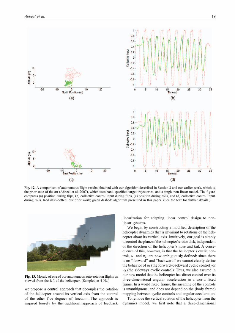
we propose a control approach that decouples the rotation

of the helicopter around its vertical axis from the control

of the other five degrees of freedom. The approach is

inspired loosely by the traditional approach of feedback

linearization for adapting linear control design to non-

linear systems.

We begin by constructing a modified description of the

helicopter dynamics that is invariant to rotations of the heli-

copter about its vertical axis. Intuitively, our goal is simply

to control the plane of the helicopter’s rotor disk, independent

of the direction of the helicopter’s nose and tail. A conse-

quence of this, however, is that the helicopter’s cyclic con-

trols, u1 and u2, are now ambiguously defined: since there

is no ‘‘forward’’ and ‘‘backward’’ we cannot clearly define

the behavior of u1 (the forward–backward cyclic control) or

u2 (the sideways cyclic control). Thus, we also assume in

our new model that the helicopter has direct control over its

three-dimensional angular acceleration in a world fixed

frame. In a world fixed frame, the meaning of the controls

is unambiguous, and does not depend on the (body frame)

mapping between cyclic controls and angular acceleration.

To remove the vertical rotation of the helicopter from the

dynamics model, we first note that a three-dimensional

Fig. 12. A comparison of autonomous flight results obtained with our algorithm described in Section 2 and our earlier work, which is

the prior state of the art (Abbeel et al. 2007), which uses hand-specified target trajectories, and a single non-linear model. The figure

compares (a) position during flips, (b) collective control input during flips, (c) position during rolls, and (d) collective control input

during rolls. Red dash-dotted: our prior work; green dashed: algorithm presented in this paper. (See the text for further details.)

Fig. 13. Mosaic of one of our autonomous auto-rotation flights as

viewed from the left of the helicopter. (Sampled at 4 Hz.)

Abbeel et al. 19

–4 –2 0 2 4 6700

750

800

850

900

950

1000

1050

1100

1150

1200

Time (s)

RPM

–4 –2 0 2 4 6750

800

850

900

950

1000

1050

1100

1150

1200

Time (s)

RPM

(e)(a)

–4 –2 0 2 4 6–5

0

5

10

15

20

25

30

35

Time (s)

Alti

tude

(m

)

–4 –2 0 2 4 60

5

10

15

20

25

30

Time (s)

Alti

tude

(m

)

(f)(b)

–4 –2 0 2 4 60

2

4

6

8

10

12

X V

eloc

ity (

m)

Time (s)–4 –2 0 2 4 60

1

2

3

4

5

6

7

8

9

X V

eloc

ity (

m)

Time (s)(g)(c)

–4 –2 0 2 4 6–30

–25

–20

–15

–10

–5

0

5

10

15

20

Time (s)

Pitc

h (D

egre

ss)

–4 –2 0 2 4 6–25

–20

–15

–10

–5

0

5

10

15

20

Time (s)

Pitc

h (D

egre

ss)

(h)(d)

Fig. 14. (a) Main rotor speed during autonomous auto-rotation flights. (b) Altitude of the helicopter during autonomous auto-rotation

flights. (c) Forward velocity of the helicopter during autonomous auto-rotation flights. (d) Pitch angle for the helicopter during

autonomous auto-rotation flights. (e) Main rotor speed in (closed-loop) simulation. (f) Altitude of the helicopter in (closed-loop)

simulation. (g) Forward velocity of the helicopter in (closed-loop) simulation. (h) Pitch angle for the helicopter in (closed-loop)

simulation. (See the text for further details.)

20 The International Journal of Robotics Research 00(000)

rotation can be decomposed into two rotations: a rotation that

is purely about the X - and Y -axes, and another rotation

about the Z-axis. In particular, if we consider a rotation

Dt;tþ1q (represented as a direction cosine matrix, or as a

quaternion) representing the rotation of the helicopter from

time t to time t þ 1, then we can write

Dt;tþ1q ¼ Dt;tþ1½qxyDt;tþ1½qz where it is possible to achieve

the rotation Dt;tþ1½qxy using only rotation about the X - and

Y - (lateral) axes of the helicopter at time t, and Dt;tþ1½qzcan be achieved purely by pirouetting, i.e. rotating around

the Z-axis of the helicopter at time t.

When presented with a target trajectory for the heli-

copter, we can apply the above described procedure to

eliminate any pirouetting in all time steps from t to

t þ 1. For this new target we can run Gauss–Newton LQR

(and receding horizon Gauss–Newton LQR) as used in all

previous experiments. We can similarly modify our

dynamics model to not include the pirouetting degree of

freedom. Hence in the three-dimensional angular rate con-

trol input space, only a two-dimensional subspace will

affect the dynamics. We use a cost function that does not

consider the pirouetting degree of freedom.

Finally, note that the controller in the new dynamics

model uses world-frame angular accelerations as its con-

trol inputs rather than the rudder and cyclic pitch con-

trols. As these controls offer three degrees of freedom,

our controller might seem over-actuated, since only two

degrees of freedom remain in the orientation state. How-

ever, since our dynamics model leaves the state

unchanged when applying an angular acceleration along

the helicopter’s Z-axis, and since our cost function pena-

lizes any non-zero control input, the irrelevant subspace

of controls will not be used.

With our reformulated dynamics model, we can run

Gauss–Newton LQR to acquire a controller that generates

a sequence of desired angular accelerations and, by inte-

gration, a sequence of desired angular rates in the world

frame. To execute these desired angular rates, they must

then be converted to body angular rates that can be

mapped to the helicopter’s cyclic and rudder controls

(u1, u2, and u3). Provided that the helicopter’s pirouette rate

is zero (that is, there is no yaw input, u3 ¼ 0), then the

world angular rate sequence generated by our controller

can be converted directly to body coordinates. This body

angular rate sequence is then used as the target trajectory

in a closed-loop rate controller for each axis (each designed

online using receding horizon Gauss–Newton LQR on a

single degree of freedom).

However, if we attempt to use a non-zero pirouette

rate, for instance, by locking the rudder control u3 at a

fixed value, then the situation is different. Note that the pir-

ouette rate has no direct impact on the output of our reced-

ing horizon Gauss–Newton LQR controller, which is now

designed to ignore rotation about the helicopter’s vertical

axis. However, for high pirouette rates, simply converting

the world-frame angular rates to the helicopter’s body

frame will not work correctly. During the 1/20th second

over which the helicopter’s controls are held fixed

(between control updates), the body of the helicopter is

rotating, and thus the direction in which these controls act

is changing. Hence, simply choosing controls to achieve a

fixed, body-coordinate angular rate will fail, because these

controls fail to account for the pirouette rate of the helicop-

ter. It turns out that one can compensate for this effect

rather easily. Given a target body-coordinate angular rate

in the helicopter’s X –Y plane (assuming no Z-axis rota-

tion), o�xy 2 R2, and a desired pirouette rate o�z , we can

compute a compensated target:

o�xy ¼ R � 1

2o�zDt

� �o�xy;

where RðyÞ is the 2� 2 rotation matrix that rotates a vector

by y.

Fig. 15. (a) Altitude during four autonomous auto-rotation descents. (b) Main rotor speed during four autonomous auto-rotation

descents. (See the text for further details.)

Abbeel et al. 21

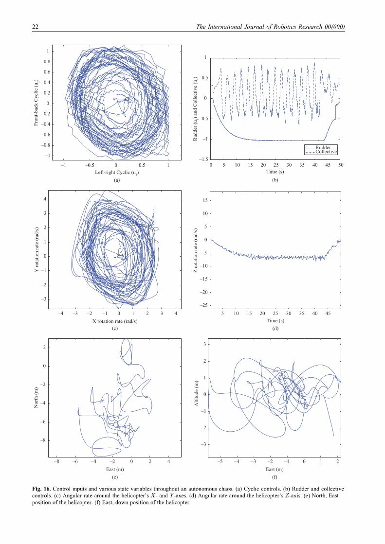
–1 –0.5 0 0.5 1

–1

–0.8

–0.6

–0.4

–0.2

0

0.2

0.4

0.6

0.8

1

Left-right Cyclic (u1)

Fron

t-ba

ck C

yclic

(u 2)

0 5 10 15 20 25 30 35 40 45 50–1.5

–1

0.5

0

0.5

1

Time (s)

Rud

der

(u3)

and

Col

lect

ive

(u4)

RudderCollective

(b)(a)

–4 –3 –2 –1 0 1 2 3 4

–3

–2

–1

0

1

2

3

4

X rotation rate (rad/s)

Y r

otat

ion

rate

(ra

d/s)

5 10 15 20 25 30 35 40 45

–25

–20

–15

–10

–5

0

5

10

15

Time (s)

Z r

otat

ion

rate

(ra

d/s)

(d)(c)

–8 –6 –4 –2 0 2 4

–8

–6

–4

–2

0

2

East (m)

Nor

th (

m)

–5 –4 –3 –2 –1 0 1 2

–3

–2

–1

0

1

2

3

East (m)

Alti

tude

(m

)

(f)(e)

Fig. 16. Control inputs and various state variables throughout an autonomous chaos. (a) Cyclic controls. (b) Rudder and collective

controls. (c) Angular rate around the helicopter’s X - and Y -axes. (d) Angular rate around the helicopter’s Z-axis. (e) North, East

position of the helicopter. (f) East, down position of the helicopter.

22 The International Journal of Robotics Research 00(000)

Using this modified control algorithm we have flown

many of our standard maneuvers, including in-place flips

and rolls, where our controllers simply follow the rotor

disk specified by the maneuver, but allow the tail direc-

tion to change over time. For instance, if we specify that

the yaw rate of the helicopter should be regulated toward

zero while performing an in-place flip, the helicopter will

flip over in place as usual, allowing the tail to drift

slowly over time eventually resulting in the body of the

helicopter flipping or rolling around different axes. This

does not change the motion of the rotor disk, however, which

continues to flip around the same axis as before. To perform

a ‘‘chaos’’, we simply select a fixed angular rate target

for the Z-axis. In our experiments, we used a target

pirouette rate of 320 per second (� 5:6 rad per second).

Figure 16 shows the state of our helicopter throughout a

sustained chaos.

10. Discussion

10.1. When Obtaining the Target Trajectory from

the Multiple Suboptimal Demonstrations, Why

Still Run the Offline Gauss–Newton LQR? Would

Offline LQR be Sufficient?

Indeed, since we learn the corrections to the model (through

the ‘‘bias’’ terms), you can, in principle, fly the trajectory

exactly according to the learned dynamics model, and hence

you only need to run the dynamic programming (LQR)

backups once. We have done this successfully.

However, after the first autonomous trial, our algorithm

incorporates the flight data to improve the dynamics model.

While in principle we could re-learn the target trajectory

while accounting for the new flight data in the dynamics

model; in practice that takes longer than is desirable in

between flights. Hence, after having incorporated the

new data (from the autonomous flight) into the dynamics

model, the target trajectory need not be flyable anymore

according to the updated dynamics model. In this setting,

Gauss–Newton LQR is not equivalent to LQR.

In addition, when we learn the locally weighted models

post-hoc from the demonstration data, this will also

break the assumption that the target trajectory is feasi-

ble—running Gauss–Newton LQR is the ‘‘safe and generic

solution’’ which covers all cases.

10.2. Is the Interpolation Between the Next State

as Predicted by the Dynamics Model and the

Target Next State Needed in the Initial Iterations

of the Offline Gauss–Newton LQR Runs to Assure

Convergence?

As our target trajectory is fairly consistent with the helicop-

ter’s dynamics, this interpolation does not matter much for

our ‘‘usual’’ airshows (slow rotation). Occasionally it pre-

vents divergence once the autonomous flight data has been

incorporated and the target trajectory has become somewhat

less consistent with this updated dynamics model.22

In earlier work, we attempted to handcode the target trajec-

tories which resulted in target trajectories that were inconsis-

tent with the helicopter dynamics. In this setting, the

interpolation greatly improved convergence of the offline runs.

10.3. Why a Two-second Receding Horizon?

Simulator experiments have shown us that a 5-s horizon

would be ideal if we had sufficient computational power

to do so in real time. In 5 s the helicopter tends to get all

the way back to the target and hence the cost-to-go at the

last time step, which is obtained from offline Gauss–

Newton LQR, is as accurate as if we would use a longer

horizon. Two seconds seemed ‘‘good enough’’ in our

simulator experiments: this usually brings the helicopter

about 80% of the way back to the target trajectory. Given

the amount of deviation we typically encounter (due to

gusts of wind, etc.), making it 80% back to the target

is sufficient for the quadratic approximation of the cost-

to-go (from the offline run) to be a reasonable approxi-

mation. There is a trade-off between more iterations in

the Gauss–Newton outer loop, a longer horizon, and the

amount of latency introduced by the computation time.

Using the 2-s horizon gave us four iterations of Gauss–

Newton LQR during the online receding horizon execu-

tion. These extra iterations might be a little overkill for

most maneuvers, but really hard maneuvers (tic-toc and

chaos) benefited substantially more from the added itera-

tions than from longer horizons.

We also performed some flight tests with varying hori-

zons: 2 s, 1 s, and 0 s (0 s means simply using the sequence

of linear feedback controllers obtained from offline Gauss–

Newton LQR). In these tests we repeatedly flew Airshow 2

on a pretty calm day (winds less than 5 mph). In each of the

three cases, the airshow was successfully completed in

repeated tests. That being said, the cost encountered

throughout the trajectory was significantly higher for

shorter horizons.

Fig. 17. Main rotor speed simulation. (See the text for further

details.)

Abbeel et al. 23

On days with more wind (e.g. 20 mph) we have

observed the receding horizon controller complete maneu-

vers that were not possible without the receding horizon.

For example, during a tic-toc, the helicopter got pushed

so far off by the wind that it had to turn inward 90 to return

to the correct position. This would not have been possible

otherwise.

10.4. What Do the Cost-to-Go Functions

Obtained from offline Gauss–Newton LQR Look

Like? Are They Trajectory Specific, or Always the

Same?

The cost-to-go matrices are fairly low rank (the top 6 eigen-

values of the cost-to-go matrix account for 97% of the sum

of all 17 eigenvalues, and this is true for most of the trajec-

tory). We inspected the dominant eigenvectors of the cost-

to-go matrix, but could not identify consistently dominant

eigenvectors or subspaces.

10.5. Are There Any Formal Robustness

Guarantees?

At the core, our feedback controllers are designed using

standard linear quadratic control design methodology;

they inherit this methodology’s robustness properties,

which includes certain gain and phase margin properties.

(See, e.g., Anderson and Moore (1989).) However, such

robustness analysis is not explicitly accounting for the

specifics of helicopter control, when one might be inter-

ested in robustness with respect to changing mass,

engine, air density, and servo properties. Moreover, the

linear quadratic analysis would not capture the improve-

ments obtained through the receding horizon aspects of

the controller. A theoretical robustness analysis is

beyond the scope of this paper. Practically speaking, our

control system appears to be nearly as reliable as a

human pilot for most of the maneuvers performed based

on the large number of successful trials the controller

has performed in actual flight and our own extensive

simulator testing. Indeed, this is the only ‘‘guarantee’’

we have for human pilots performing the same maneu-

vers. Degradation of equipment and changes in mass

and balance can affect the performance of our control-

lers. Nevertheless, significant changes are quite manage-

able: the online learning phase where the model is

adjusted based on flight data is able to remove many

errors caused by wind and modest changes in the aircraft

characteristics without the need to rebuild controllers.

This is quite comparable to human performance,

where changes to the aircraft require a short ‘‘feeling

out’’ period where the human pilot builds up muscle

memory for various maneuvers. Even without this step,

the controllers are (qualitatively) tolerant to wind and

dynamics errors though sometimes resulting in reduced

performance.

10.6. Does this Apprenticeship Learning

Approach Require Demonstrations for Every

Possible Mission to be Flown?

No. To fly an arbitrary mission, we would first use our tra-

jectory learning algorithm to learn a library of short trajec-

tories/maneuvers. We would then feed the resulting library

of short trajectories into a high-level (mission level) plan-

ner that sequences them together. To account for which

maneuvers can be executed after which other maneuvers,

one could use approaches such as those proposed by Fraz-

zoli et al. (2002, 2005).

11. Conclusion

We have presented apprenticeship learning algorithms for

learning control policies. While these algorithms are not

specific to helicopters, they have enabled us to efficiently

find high-performance controllers for the very challenging

control problem of autonomous helicopter aerobatics. Our

helicopter is the first autonomous helicopter capable of fly-

ing a very wide range of highly challenging aerobatics at

the same level as human expert pilots.

Acknowledgments

We thank Garett Oku for piloting and building our helicop-

ters. This work was supported in part by the DARPA

Learning Locomotion program under contract number

FA8650-05-C-7261. Adam Coates is supported by a Stan-

ford Graduate Fellowship.

Appendix A: Trajectory Learning Algorithm

As described in Section 2, our algorithm (approxi-

mately) solves

maxτ;Sð�Þ;d logPðy; ρ; τ ; Sð�Þ; dÞ: ð13Þ

Then, once our algorithm has found τ; d;Sð�Þ, it finds the

most likely hidden trajectory, namely the trajectory z that

maximizes the joint likelihood of the observed trajectories

y and the observed prior knowledge about the ideal trajec-

tory ρ for the learned parameters τ; d;Sð�Þ. To optimize

Equation (13), we alternatingly optimize over Sð�Þ, d, and

τ. Section 4.2 provides the high-level description, below

we provide the detailed description of our algorithm.

1. Initialize the parameters to hand-chosen defaults.

A typical choice: Sð�Þ ¼ I ; dki ¼ 1

3;

τkj ¼ j T�1

Nk�1:

2. E-step for latent trajectory: for the current setting of

τ;Sð�Þ run a (extended) Kalman smoother to find the

distributions for the latent states, NðmtjT�1;StjT�1Þ.3. M-step for latent trajectory: update the covariances

Sð�Þ using the standard EM update.

4. E-step for the time indexing (using hard assignments):

run dynamic time warping to find τ that maximizes the

joint probability Pðz; y; r; τÞ, where z is fixed to mtjT�1,

24 The International Journal of Robotics Research 00(000)

namely the mode of the distribution obtained from the

Kalman smoother.

5. M-step for the time indexing: estimate d from τ.

6. Repeat steps 2–5 until convergence.

A.1 Steps 2 and 3 Details: EM for Non-linear Dynamical

Systems

Steps 2 and 3 in our algorithm correspond to the

standard E and M steps of the EM algorithm applied

to a non-linear dynamical system with Gaussian

noise. For completeness we provide the details below.

In particular, we have

ztþ1 ¼ f ðztÞ þ ot; ot � Nð0;QÞ;

ytþ1 ¼ hðztÞ þ nt; nt � Nð0;RÞ:

In the E-step, for t ¼ 0; . . . ; T � 1, the Kalman smoother

computes the parameters mtjt and Stjt for the distribution

Nðmtjt;StjtÞ, which is the distribution of zt conditioned on

all observations up to and including time t. Along the way,

the smoother also computes mtþ1jt and Stþ1jt. These are the

parameters for the distribution of ztþ1 given only the

measurements up to time t. Finally, during the backward

pass, the parameters mtjT�1 and StjT�1 are computed, which

give the distribution for zt given all measurements.

After running the Kalman smoother (for the

E-step), we can use the computed quantities to updateQ and R in the M-step. In particular, we can compute23

dmt ¼ mtþ1jT�1 � f ðmtjT�1Þ;At ¼ Df ðmtjT�1Þ;Lt ¼ StjtA

Tt S�1tþ1jt;

Pt ¼ Stþ1jT�1 � Stþ1jT�1LTt AT

t � AtLtStþ1jT�1;

Q ¼ 1

T

XT�1

t¼0

dmtdmTt þ AtStjT�1AT

t þ Pt;

dyt ¼ yt � hðmtjT�1Þ;Ct ¼ DhðmtjT�1Þ;

R ¼ 1

T

XT�1

t¼0

dytdyTt þ CtStjT�1CT

t :

A.2 Steps 4 and 5 Details: Dynamic Time Warping

In Step 4 our goal is to compute �t as

�τ ¼ arg maxτ logPð�z; y; ρ; τ;Sð�Þ; dÞ¼ arg maxτ logPðyj�z; τÞPðρj�zÞPð�zÞPðτÞ¼ arg maxτ logPðyjz; τÞPðτÞ;

ð14Þ

where z is the mode of the distribution computed by the

Kalman smoother (namely, �zt ¼ mtjT�1) and Equation (14)

made use of independence assumptions implied by our

model (see Figure 3). Again, using independence proper-

ties, the log likelihood above can be expanded to

�τ ¼ arg maxτXM�1

k¼0

XNk�1

j¼0

‘ðykj j�zτk

j; τk

j Þ þ ‘ðτkj jτk

j�1Þh i

: ð15Þ

Note that the inner summations in the above expression are

independent: the likelihoods for each of the M observation

sequences can be maximized separately. Hence, in the fol-

lowing, we omit the k superscript, as the algorithm can be

applied separately for each sequence of observations and

indices.

At this point, we can solve the maximization over τusing a dynamic programming algorithm known in the

speech recognition literature as dynamic time warping

(Sakoe and Chiba 1978) and in the biological sequence

alignment literature as the Needleman–Wunsch algorithm

(Needleman and Wunsch 1970). For completeness, we pro-

vide the details for our setting below.

We define the quantity Qðs; tÞ to be the maximum

obtainable value of the first sþ 1 terms of the inner sum-

mation if we choose τs ¼ t.

For s ¼ 0, we have

Qð0; tÞ ¼ ‘ðy0j�zτ0; τ0 ¼ tÞ þ ‘ðτ0 ¼ tÞ; ð16Þ

and for s > 0,

Qðs; tÞ ¼ ‘ðysj�zτs; τs ¼ tÞ

þmaxτ1;...;τs�1‘ðτs ¼ tjτs�1Þ½

þXs�1

j¼0

½‘ðyjj�zτj; τjÞ þ ‘ðτjjτj�1Þ:

ð17Þ

The latter equation can be written recursively as

Qðs; tÞ ¼ ‘ðysj�zτs; τs ¼ tÞ

þmaxt0 ‘ðτs ¼ tjτs�1 ¼ t0Þ þ Qðs� 1; t0Þ½ :ð18Þ

Equations (16) and (18) can be used to compute

maxtQðN k � 1; tÞ for each observation sequence (and the

maximizing solution, τ), which is exactly the maximizing

value of the inner summation in Equation (15). The maxi-

mization in Equation (18) can be restricted to the relevant

values of t0. In our application, we only allow

t0 2 ft � 3; t � 2; t � 1g. As is common practice, we typi-

cally restrict the time-index assignments to a fixed-width

band around the default, equally spaced alignment. In our

case, we only compute Qðs; tÞ if 2s� C � t � 2sþ C, for

fixed C.

In Step 5 we compute the parameters d using stan-

dard maximum-likelihood estimates for multinomial

distributions.

Appendix B: Helicopter Model During

Auto-rotation

During auto-rotation, we use the following model

structure:

Abbeel et al. 25

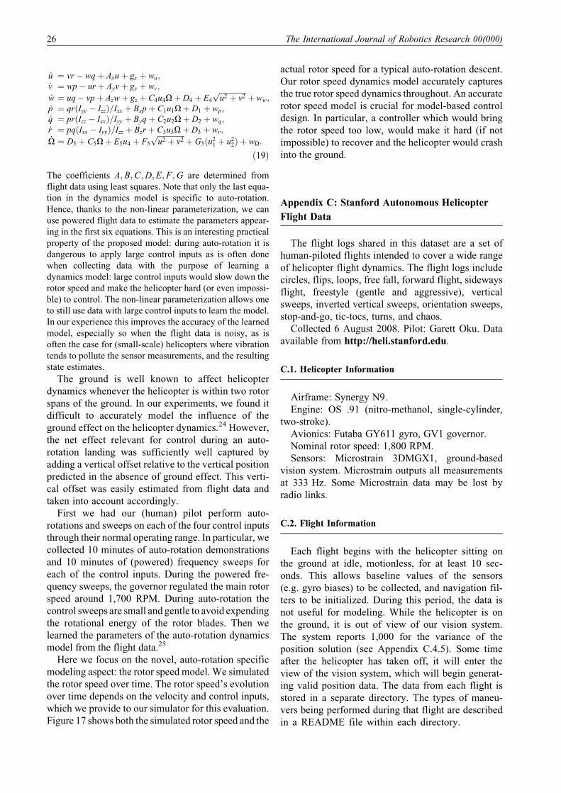
_u ¼ vr � wqþ Axuþ gx þ wu;_v ¼ wp� ur þ Ayvþ gy þ wv;

_w ¼ uq� vpþ Azwþ gz þ C4u4Oþ D4 þ E4

ffiffiffiffiffiffiffiffiffiffiffiffiffiffiffiu2 þ v2p

þ ww;_p ¼ qrðIyy � IzzÞ=Ixx þ Bxpþ C1u1Oþ D1 þ wp;_q ¼ prðIzz � IxxÞ=Iyy þ Byqþ C2u2Oþ D2 þ wq;_r ¼ pqðIxx � IyyÞ=Izz þ Bzr þ C3u3Oþ D3 þ wr;_O ¼ D5 þ C5Oþ E5u4 þ F5

ffiffiffiffiffiffiffiffiffiffiffiffiffiffiffiu2 þ v2p

þ G5ðu21 þ u2

2Þ þ wO:

ð19Þ

The coefficients A;B;C;D;E;F;G are determined from

flight data using least squares. Note that only the last equa-

tion in the dynamics model is specific to auto-rotation.

Hence, thanks to the non-linear parameterization, we can

use powered flight data to estimate the parameters appear-

ing in the first six equations. This is an interesting practical

property of the proposed model: during auto-rotation it is

dangerous to apply large control inputs as is often done

when collecting data with the purpose of learning a

dynamics model: large control inputs would slow down the

rotor speed and make the helicopter hard (or even impossi-

ble) to control. The non-linear parameterization allows one

to still use data with large control inputs to learn the model.

In our experience this improves the accuracy of the learned

model, especially so when the flight data is noisy, as is

often the case for (small-scale) helicopters where vibration

tends to pollute the sensor measurements, and the resulting

state estimates.

The ground is well known to affect helicopter

dynamics whenever the helicopter is within two rotor

spans of the ground. In our experiments, we found it

difficult to accurately model the influence of the

ground effect on the helicopter dynamics.24 However,

the net effect relevant for control during an auto-

rotation landing was sufficiently well captured by

adding a vertical offset relative to the vertical position

predicted in the absence of ground effect. This verti-

cal offset was easily estimated from flight data and

taken into account accordingly.

First we had our (human) pilot perform auto-

rotations and sweeps on each of the four control inputs

through their normal operating range. In particular, we

collected 10 minutes of auto-rotation demonstrations

and 10 minutes of (powered) frequency sweeps for

each of the control inputs. During the powered fre-

quency sweeps, the governor regulated the main rotor

speed around 1,700 RPM. During auto-rotation the

control sweeps are small and gentle to avoid expending

the rotational energy of the rotor blades. Then we

learned the parameters of the auto-rotation dynamics

model from the flight data.25

Here we focus on the novel, auto-rotation specific

modeling aspect: the rotor speed model. We simulated

the rotor speed over time. The rotor speed’s evolution

over time depends on the velocity and control inputs,

which we provide to our simulator for this evaluation.

Figure 17 shows both the simulated rotor speed and the

actual rotor speed for a typical auto-rotation descent.

Our rotor speed dynamics model accurately captures

the true rotor speed dynamics throughout. An accurate

rotor speed model is crucial for model-based control

design. In particular, a controller which would bring

the rotor speed too low, would make it hard (if not

impossible) to recover and the helicopter would crash

into the ground.

Appendix C: Stanford Autonomous Helicopter

Flight Data

The flight logs shared in this dataset are a set of

human-piloted flights intended to cover a wide range

of helicopter flight dynamics. The flight logs include

circles, flips, loops, free fall, forward flight, sideways

flight, freestyle (gentle and aggressive), vertical

sweeps, inverted vertical sweeps, orientation sweeps,

stop-and-go, tic-tocs, turns, and chaos.

Collected 6 August 2008. Pilot: Garett Oku. Data

available from http://heli.stanford.edu.

C.1. Helicopter Information

Airframe: Synergy N9.

Engine: OS .91 (nitro-methanol, single-cylinder,

two-stroke).

Avionics: Futaba GY611 gyro, GV1 governor.

Nominal rotor speed: 1,800 RPM.

Sensors: Microstrain 3DMGX1, ground-based

vision system. Microstrain outputs all measurements

at 333 Hz. Some Microstrain data may be lost by

radio links.

C.2. Flight Information

Each flight begins with the helicopter sitting on

the ground at idle, motionless, for at least 10 sec-

onds. This allows baseline values of the sensors

(e.g. gyro biases) to be collected, and navigation fil-

ters to be initialized. During this period, the data is

not useful for modeling. While the helicopter is on

the ground, it is out of view of our vision system.

The system reports 1,000 for the variance of the

position solution (see Appendix C.4.5). Some time

after the helicopter has taken off, it will enter the

view of the vision system, which will begin generat-

ing valid position data. The data from each flight is

stored in a separate directory. The types of maneu-

vers being performed during that flight are described

in a README file within each directory.

26 The International Journal of Robotics Research 00(000)

C.3. Log Files

Each directory contains a set of ASCII text files.

The contents of each file are:

� comments.txt: comments from the software operator

during the flight.

� controls.txt: pilot controls.

� filter.txt: state estimate from the flight software’s

Kalman filter.

� imuaccel.txt: acceleration from Microstrain unit.

� imugyro.txt: angular rate from Microstrain unit.

� imumag.txt: magnetic field measurements from Micro-

strain unit.

� smoother.txt: state estimate from Kalman smoother

(post-processed).

� vision.txt: measurements from ground-based vision.

� logfile.txt: interleaved (by time) data from all files.

C.4. Formats

Each file is a sequence of tuples separated by

newlines. The first entry of each line is a digit iden-

tifying the type of data to follow. logfile.txt contains

all of the data, and thus each line may have a differ-

ent format. The data has been separated out (based

on the leading type digit) into the other files for

simplicity.

0 Comment

1 IMU accelerometers

2 IMU gyros

3 IMU magnetometers

The type of

data associated

with each digit is:

4 Vision

5 Controls

6 Filter

7 Smoother

Each tuple has one of the following formats,

depending on the leading digit.

C.4.1. Comments

0 time comment_text

time:time in seconds. This is the time at which the

comment was entered into the software by the opera-

tor and may only roughly correspond to the event

referred to in the text.

comment_text:all remaining text on the line

(including spaces) is the comment text entered by the

operator.

C.4.2. IMU Accelerometers

1 time accel_x accel_y accel_z

time:time in seconds. This is the time at which the

measurement was processed by the software (not

necessarily when it was sensed).

accel_x: acceleration in meters per second per

second along the helicopter’s local X -axis (forward).

accel_y: acceleration in meters per second per

second along the helicopter’s local Y -axis (right).

accel_z: acceleration in meters per second per

second along the helicopter’s local Z-axis (down).

C.4.3. IMU Gyros

2 time rate_x rate_y rate_z

time:time in seconds. This is the time at which the

measurement was processed by the software (not

necessarily when it was sensed).

rate_x: angular rate in radians per second

around the helicopter’s local X -axis (forward).

rate_y: angular rate in radians per second around

the helicopter’s local Y -axis (right).

rate_z: angular rate in radians per second around

the helicopter’s local Z-axis (down).

C.4.4. IMU Magnetometers

3 time field_x field_y field_z

time:time in seconds. This is the time at which the

measurement was processed by the software (not

necessarily when it was sensed).

field_x: magnetic field strength in Gauss along

the helicopter’s local X -axis (forward).

field_y: magnetic field strength in Gauss along

the helicopter’s local Y -axis (right).

field_z: magnetic field strength in Gauss along the

helicopter’s local Z-axis (down).

Units may not be exactly Gauss. The local mag-

netic variation at the flying field is approximately15:5 (0.27 rad) East. The local magnetic dip at the flying

field is approximately 62.

C.4.5. Vision

4 time pos_n pos_e pos_d var_n var_e var_d

cam0_u cam0_v cam0_n cam0_e cam0_d cam1_u

cam1_v cam1_n cam1_e cam1_d

time: time in seconds. Time at which the measure-

ment was processed by software.

pos_n/e/d: three-dimensional position in the navi-

gation frame (North–East–down), measured in

meters. North refers to true North, not magnetic.

Abbeel et al. 27

var_n/e/d: variance of the position solution. Gener-

ally the fitting error is very small and, unfortunately,

does not reflect actual accuracy.

If the helicopter is currently not being tracked (out

of the camera view, or lost track), these values are set

to 1,000. The Kalman filter/smoother data may be

unreliable during this time (and shortly before/after

depending on the nature of the outage).

cam0_u/v: U ;V coordinates of helicopter in camera 0’s

image.

cam0_n/e/d: a vector pointing from camera

0’s focal point to the helicopter, expressed in the

North–East–down frame.

cam1_u/v: U ;V coordinates of helicopter in camera 1’s

image.

cam1_n/e/d: a vector pointing from camera 1’s

focal point to the helicopter, expressed in the

North–East–down frame.

The vision system consists of two cameras mounted

at fixed locations on the field. Intrinsic parameters

(principal point and focal lengths) were determined

by standard methods. Their extrinsic parameters were

calibrated using location data from a high-accuracy

GPS unit appearing in the camera views.

Each camera outputs a 640� 480 image. The U ;Vcoordinates are image coordinates of the helicopter: U spe-

cifies the column and V specifies the row within the image

(starting from the top-left corner of the image). These U ;Vcoordinates are converted (using intrinsic parameters) to a

local three-dimensional ray, then rotated to the nav frame,

yielding the cam*_n/e/d vectors. Along with the positions

of the cameras in the North–East–down frame, these navi-

gation frame rays are intersected (least squares) to find the

three-dimensional position of the helicopter.

The intrinsic parameters for the cameras are

Camera 0 U V

Focal length 1,142.4746 1,140.8725

Principal point 328.14 231.89

Camera 1 U VFocal length 1,043.9616 1,043.3972

Principal point 319.5 239.5

The extrinsic parameters for the cameras are

Camera 0

Rotation vector �1.3898633 �1.6186237 �1.0987801Translation

vector

8.7648435 4.7797100 4.752933

Camera 1

Rotation vector �1.6861621 �1.2023404 �0.86853279Translation

vector�9.1579315 5.8206285 12.334456

The rotation vectors are axis-angle rotations of

the navigation frame relative to the camera (see

cvRodrigues2 in the OpenCV Library documentation).

The translation vectors are the position of the origin

expressed in the camera frame.

C.4.6. Controls

5 time aileron elevator rudder collective

time: time in seconds. Time at which the measure-

ment was processed by software.

aileron: aileron (lateral cyclic) stick position. The

lateral cyclic controls the helicopter’s left–right tilt

(roll). This is the horizontal axis of the pilot’s right

stick.

elevator: elevator (longitudinal cyclic) stick posi-

tion. The longitudinal cyclic controls the helicopter’s

forward–backward tilt (pitch). This is the vertical axis

of the pilot’s right stick.

rudder: rudder stick position. The rudder controls

the helicopter’s rotational rate about its vertical axis

(yaw). This is the horizontal axis of the pilot’s left

stick.

collective: collective stick position. The collective

controls the main rotor collective pitch, increasing

and decreasing vertical thrust. This is the vertical axis

of the pilot’s left stick.

Each control is normalized approximately to the

range ½�1;þ1 (it should be considered unsafe to exceed

this range under computer control). Positive aileron

corresponds to a positive rotational rate about the

helicopter’s X - (forward) axis, and a right stick deflection.

Positive elevator corresponds to a negative rotational rate

about the helicopter’s Y - (right) axis, and an upward stick

deflection. Positive rudder corresponds to a positive rota-

tion rate about the helicopter’s Z- (down) axis (hence,

clockwise viewed from above). This corresponds to a right

stick deflection. Positive collective corresponds to an

upward blade pitch (zero pitch corresponds to the 0 posi-

tion), which generates upward thrust (along the negative

Z-axis). This corresponds to upward stick deflection.

Copies of the servo commands sent to the helicop-

ter are received by a second radio receiver attached to

the flight computer. These servo positions are mixed

together by our Futaba transmitter and, thus, not direct

measurements of the pilot’s controls. The controls in

the log file are ‘‘unmixed’’ by inverting the mixing

process applied by the transmitter.

C.4.7. Filter

6 time pos_n pos_e pos_d q_x q_y q_z q_w vel_n

vel_e vel_d w_n w_e w_d vdot_n vdot_e vdot_d

wdot_n wdot_e wdot_d euler_roll euler_pitch

euler_yaw

time: Time in seconds at which the filter estimate

was computed.

28 The International Journal of Robotics Research 00(000)

pos_n/e/d: Estimated position of the helicopter in

the North–East–down frame, measured in meters.

q_x/y/z/w: Quaternion representation of the

helicopter’s orientation relative to the North–East–

down frame. The quaternion 0,0,0,1 corresponds to

the helicopter having its X -axis aligned with North, Y -

axis aligned with East, and Z-axis aligned with down.

vel_n/e/d: the helicopter’s linear velocity in meters

per second in the North–East–down frame.

w_n/e/d: the helicopter’s angular velocity in

radians per second in the North–East–down frame.

vdot_n/e/d: the helicopter’s linear acceleration in

meters per second per second in the North–East–down

frame.

wdot_n/e/d: the helicopter’s angular acceleration in

radians per second per second in the North–East–

down frame.

euler_roll: roll angle of the helicopter in radians.

euler_pitch: pitch angle of the helicopter in radians.

euler_yaw: yaw angle (heading) of the helicopter in

radians.

The euler angles are included for human readability

and sanity checking. Rotations are done in roll–pitch–

yaw order (standard aviation convention). Note that

small rotations in roll, pitch, or yaw from the starting

orientation (level, facing North) correspond to posi-

tive rotations about the North, East, down axes.

Note that many references differ in their quaternion

conventions. The following matrix transformation is

equivalent to the rotation represented by a quaternionðx; y; z;wÞ:

R(x,y,z,w) ¼[1-2yy-2zz, 2xy - 2zw, 2xz þ 2yw]

[2xy þ 2zw, 1-2xx-2zz, 2yz - 2xw]

[2xz - 2yw, 2yz þ 2xw, 1-2xx-2yy]

This rotation matrix, when applied to a vector ‘‘v’’

expressed in the helicopter frame results in a vector

expressed in the navigation frame. Alternatively, the trans-

formation is the operator which rotates the helicopter from

the default orientation (level, facing North) to the orienta-

tion represented by the quaternion ðx; y; z;wÞ. Comparing

this with other conventions will often avoid confusion

and/or mixing of incompatible code.

C.4.8. Smoother

7 time pos_n pos_e pos_d q_x q_y q_z q_w vel_n

vel_e vel_d w_n w_e w_d vdot_n vdot_e vdot_d

wdot_n wdot_e wdot_d euler_roll euler_pitch euler_

yaw

Same format as Filter data.

Notes

1. In a bit more detail: the main rotor pitch angle can be expressed

u4+u1 sin y + u2 cos y as where y is the phase of the main rotor

in its rotation around the vertical axis of the helicopter. The

pitch angle of the main rotor affects the force generated by the

main rotor, which, through the main rotor hub and shaft, results

in pitch and roll torques being exerted on the helicopter.

2. The state transition model also predicts the controls as a func-

tion of the previous state and controls. In our experiments we

predict u�tþ1 as u�t plus Gaussian noise.

3. Even though our observations, y, are correlated over time

with each other due to the dynamics governing the observed

trajectory, our model assumes that the observations y kj are

independent for all j ¼ 0; . . . ; Nk � 1 and k ¼ 0 . . . ; M � 1.

4. Our generative model can incorporate richer local models.

We discuss our choice of merely using biases in our genera-

tive trajectory model in more detail in Section 5.

5. Note that maximizing over the hidden trajectory and the cov-

ariance parameters simultaneously introduces undesirable

local maxima: the likelihood score would be highest (namely

infinity) for a hidden trajectory with a sequence of states

exactly corresponding to the (crude) dynamics model f (�) and

state-transition covariance matrices equal to all-zeros as long

as the observation covariances are non-zero. Hence, we mar-

ginalize out the hidden trajectory to find τ, d, Sð�Þ.6. Fixing z means the dynamic time-warping step only approx-

imately optimizes the original objective. Unfortunately, with-

out fixing z, the independencies required to obtain an efficient

dynamic programming algorithm do not hold. In practice, we

find our approximation works very well.

7. During real-time control execution, our model is queried

roughly 52,000 times per second. Even with KD-tree

(Preparata and Shamos 1985; Moore et al. 1997) or cover-

tree Beygelzimer et al. 2006) data structures a full locally

weighted model would be much too slow.

8. In practice, the data points along a short segment of the trajec-

tory lie in a low-dimensional subspace of the state space. This

sometimes leads to an ill-conditioned parameter estimation

problem. To mitigate this problem, we regularize our models

toward the ‘‘crude’’ model f (�). Or, in other words, we learn a

correction to the crude model.

9. We could learn the richer local model within the trajectory

alignment algorithm, updating the dynamics model during the

M-step. We chose not to do so since these models are more

computationally expensive to estimate. The richer models have

minimal influence on the alignment because the biases capture

the average model error: the richer models capture the deriva-

tives around it. Given the limited influence on the alignment,

we chose to save computational time and only estimate the

richer models after alignment.

10. In prior work we have referred to our control approach as

DDP. However, technically, we have always used Gauss–

Newton LQR.

11. See, e.g., Randlov and Alstrom (1998) for another example of

homotopy/continuation methods applied in reinforcement

learning.

12. When adding the integrated error in position to the cost we

did not experience any benefits. Even worse, when increasing

its weight in the cost function, the resulting controllers were

often unstable. This could be related to the helicopter being

underactuated: it can only directly compensate for position

error in the direction of its vertical thrust. Moreover, this

Abbeel et al. 29

direction changes over time as the helicopter’s orientation

changes over time.

13. The high-frequency noise on the IMU measurements is

caused by the vibration of the helicopter. This vibration is

mostly caused by the blades spinning at 30 Hz.

14. This port is known as a ‘‘buddy port’’, and is a standard com-

ponent of most hobby transmitters. It is usually used for train-

ing human pilots.

15. One must choose these somewhat carefully, since some

extreme control stick positions can saturate the servo outputs,

which would result in a non-linear mapping.

16. Special care must be taken for the throttle servo mapping,

which is often a ‘‘V’’-shaped function rather than linear func-

tion (for aerobatics). Typically, the throttle PWM value is a

piecewise linear function of the collective, which is easily

determined from the captured data.

17. For implementational convenience, we use numerical (finite-

difference) linearizations of the non-linear measurement and

dynamics functions.

18. These are the position coordinates projected into a plane

orthogonal to the axis of rotation.

19. While engine failure is one reason to fly a helicopter in auto-

rotation, auto-rotation is also crucial in the case of tail-rotor

failure. In the case of tail-rotor failure, if one keeps the engine

running, the torque from the engine causes the helicopter to

rotate (quickly) around its vertical axis, which makes it very

hard (if not impossible) to fly the helicopter reliably. Switch-

ing off the engine removes the torque that causes this rotation.

Hence, in the case of tail rotor failure, the pilot can still main-

tain control of the helicopter by disengaging the engine and

performing an auto-rotation descent and landing.

20. Indeed, in principle it might have seemed a natural choice to

just use the slowest demonstrated flare. However, there is a

big discrepancy between sensing capabilities of our autono-

mous helicopter and our expert pilot. In particular, our expert

pilot has better accuracy in sensing the distance of the heli-

copter from the ground. On the other hand, our autonomous

helicopter has better rotor speed sensing accuracy. As a con-

sequence, the naturally safest auto-rotation trajectories are

different for our expert pilot and our autonomous helicopter.

Our expert pilot prefers the helicopter to have high velocity,

and can then time his controls just right relative to the ground

to transfer (forward) velocity into rotor speed when pitching

back during the flare. By contrast, our autonomous helicopter

can more accurately maintain rotor speed during the descent.

Hence, it does not need as much forward velocity to ensure

sufficient rotor speed in the flare and landing phase. As a con-

sequence, the safer approach for our autonomous helicopter is

to execute a slowed-down version of our expert’s auto-

rotation.

21. The engine is not actually turned off. Instead, the throttle is

reduced to idle, causing the clutch attached to the main rotor

to disengage. In this state the main rotor spins freely and is no

longer driven by the engine.

22. In principle we could of course re-learn the target trajectory to

ensure consistency with the updated dynamics model, but this

would take several minutes of computational time between

flight trials. Right now, it takes of the order of seconds to

incorporate the new flight data and build the corresponding

controller. Hence, our current setup allows us to run several

flight tests in one tank of gas (about 8 minutes of flight time

per tank of gas), which greatly increases the amount of flight

testing we can perform.

23. The notation Df ðzÞ is the Jacobian of f evaluated at z.

24. Close to the ground, one cannot safely exert the large control

inputs standardly used to collect flight data for system

identification.

25. The parameters we found for our helicopter were: Ax=�0.05;

Ay =�0.06; [Az; C4; D4; E4] = [�1.42;� 0.01;�0.47;�0.15];

[Bx; C1; D1] = [�5.74; 0.02; �1.46]; [By; C2; D2] = [�5.32;

�0.01; �0.23]; [Bz; C3; D3] = [�5.43; 0.02; 0.52]; [D5; C5;

E5;F5; G5] = [106.85; �0.23; �68.53; 22.79; 2.11;�6.10].

References

Abbeel, P., Coates, A., Hunter, T. and Ng, A. Y. (2008). Autono-

mous auto-rotation of an RC helicopter. Proceedings of ISER.

Abbeel, P., Coates, A., Quigley, M. and Ng, A. Y. (2007). An

application of reinforcement learning to aerobatic helicopter

flight. Proceedings of NIPS 19.

Abbeel, P., Ganapathi, V. and Ng, A. Y. (2006a). Learning vehi-

cular dynamics with application to modeling helicopters. Pro-

ceedings of NIPS 18.

Abbeel, P. and Ng, A. Y. (2004). Apprenticeship learning via

inverse reinforcement learning. Proceedings of ICML.

Abbeel, P. and Ng, A. Y. (2005a). Exploration and apprenticeship

learning in reinforcement learning. Proceedings of ICML.

Abbeel, P. and Ng, A. Y. (2005b). Learning first order Markov

models for control. Proceedings of NIPS 18.

Abbeel, P., Quigley, M., and Ng, A. Y. (2006b). Using inaccurate

models in reinforcement learning. Proceedings of ICML.

An, C. H., Atkeson, C. G. and Hollerbach, J. M. (1988). Model-

Based Control of a Robot Manipulator. Cambridge, MA, MIT

Press.

Anderson, B. and Moore, J. (1989). Optimal Control: Linear

Quadratic Methods. Englewood Cliffs, NJ, Prentice-Hall.

Atkeson, C. G., Moore, A. W. and Schaal, S. (1997). Locally

weighted learning for control. Artificial Intelligence Review,

11(1–5).

Atkeson, C. G. and Schaal, S. (1997). Robot learning from

demonstration. Proceedings of the 14th International Confer-

ence on Machine Learning. San Mateo, CA, Morgan

Kaufmann, pp. 12–20.

Bagnell, J. and Schneider, J. (2001). Autonomous helicopter con-

trol using reinforcement learning policy search methods. Inter-

national Conference on Robotics and Automation. Piscataway,

NJ, IEEE Press.

Bar-Itzhack, I. Y. and Oshman, Y. (1985). Attitude determination

from vector observations: Quaternion estimation. IEEE Trans-

action on Aerospace and Electronic Systems.

Bertsekas, D. P. (2001). Dynamic Programming and Optimal

Control, volume 1, 2nd edn. New York, Athena Scientific.

Beygelzimer, A., Kakade, S. and Langford, J. (2006). Cover trees

for nearest neighbor. ICML ‘06: Proceedings of the 23rd Inter-

national Conference on Machine Learning.

Boutilier, C., Friedman, N., Goldszmidt, M. and Koller, D.

(1996). Context-specific independence in Bayesian networks.

Proceedings of UAI.

30 The International Journal of Robotics Research 00(000)

Calinon, S., Guenter, F. and Billard, A. (2007). On learning, rep-

resenting and generalizing a task in a humanoid robot. IEEE

Transaction on Systems, Man, and Cybernetics, Part B, 37.

Coates, A., Abbeel, P. and Ng, A. Y. (2008). Learning for control

from multiple demonstrations. Proceedings of ICML.

Dempster, A. P., Laird, N. M. and Rubin, D. B. (1977). Maximum

likelihood from incomplete data via the EM algorithm. Jour-

nal of the Royal Statistical Society.

Frazzoli, E., Dahleh, M. and Feron, E. (2002). Real-time motion

planning for agile autonomous vehicles. AIAA Journal on Gui-

dance, Control and Dynamics.

Frazzoli, E., Dahleh, M. and Feron, E. (2005). Maneuver-based

motion planning for nonlinear systems with symmetries. IEEE

Transactions on Robotics.

Gavrilets, V., Martinos, I., Mettler, B. and Feron, E. (2002a). Con-

trol logic for automated aerobatic flight of miniature helicop-

ter. AIAA Guidance, Navigation and Control Conference.

Gavrilets, V., Martinos, I., Mettler, B. and Feron, E. (2002b).

Flight test and simulation results for an autonomous aerobatic

helicopter. AIAA/IEEE Digital Avionics Systems Conference.

Gavrilets, V., Martinos, M., Mettler, B. and Feron, E. (2002c).

Control logic for automated aerobatic flight of miniature heli-

copter. Proceedings of the AIAA Guidance, Navigation, and

Control Conference.

Gelb, A. (ed.) (1974). Applied Optimal Estimation. Cambrdige,

MA, MIT Press.

Jacobson, D. H. and Mayne, D. Q. (1970). Differential Dynamic

Programming. Amsterdam, Elsevier.

Johnson, W. (1977). Helicopter Optimal Descent and Landing

After Power Loss. Report NASA TM-73244.

Kalman, R. E. (1960). A new approach to linear filtering and pre-

diction problems. Transactions of the ASME–Journal of Basic

Engineering (Series D), 82: 35–45.

La Civita, M., Messner, W. C. and Kanade, T. (2002). Modeling

of small-scale helicopters with integrated first-principles and

system-identification techniques. Proceedings of the 58th

Forum of the American Helicopter Society.

La Civita, M., Papageorgiou, G., Messner, W. C. and Kanade,

T. (2003). Design and flight testing of a gain-scheduled

H-infinity loop shaping controller for wide-envelope flight

of a robotic helicopter. Proceedings of the American Control

Conference.

La Civita, M., Papageorgiou, G., Messner, W. C. and Kanade, T.

(2006). Design and flight testing of a high-bandwidthH1 loop

shaping controller for a robotic helicopter. Journal of Gui-

dance, Control, and Dynamics, 29(2): 485–494.

Lee, A. (1985). Optimal Landing of a Helicopter in Autorotation.

PhD Thesis, Stanford University.

Lefferts, E., Markley, F. L. and Shuster, M. D. (1982). Kalman fil-

tering for spacecraft attitude estimation. Journal of Guidance,

Control, and Dynamics.

Leishman, J. (2000). Principles of Helicopter Aerodynamics.

Cambridge, Cambridge University Press.

Listgarten, J. (2006). Analysis of Sibling Time Series Data: Align-

ment and Difference Detection. PhD Thesis, University of

Toronto.

Listgarten, J., Neal, R. M., Roweis, S. T. and Emili, A. (2005).

Multiple alignment of continuous time series. Proceedings of

NIPS 17.

Mettler, B., Tischler, M. and Kanade, T. (1999). System identifi-

cation of small-size unmanned helicopter dynamics. American

Helicopter Society, 55th Forum.

Moore, A., Schneider, J. and Deng, K. (1997). Efficient locally

weighted polynomial regression predictions. Proceedings of

ICML.

Neal, R. and Hinton, G. (1999). A view of the EM algorithm

that justifies incremental, sparse, and other variants. Learn-

ing in Graphical Models. Cambrdige, MA, MIT Press, pp.

355–368.

Needleman, S. and Wunsch, C. (1970). A general method applica-

ble to the search for similarities in the amino acid sequence of

two proteins. Journal of Molecular Biology.

Neu, G. and Szepesvari, C. (2007). Apprenticeship learning using

inverse reinforcement learning and gradient methods. Pro-

ceedings of UAI.

Ng, A. Y., Coates, A., Diel, M., Ganapathi, V., Schulte, J., Tse, B.,

Berger, E. and Liang, E. (2004a). Autonomous inverted heli-

copter flight via reinforcement learning. Proceedings of ISER.

Ng, A. Y., Kim, H. J., Jordan, M., and Sastry, S. (2004b). Autno-

nomous helicopter flight via reinforcement learning. Proceed-

ings of NIPS 16.

Ng, A. Y. and Russell, S. (2000). Algorithms for inverse reinfor-

cement learning. Proceedings of ICML.

Preparata, F. P. and Shamos, M. (1985). Computational Geome-

try. Berlin, Springer-Verlag.

Ramachandran, D. and Amir, E. (2007). Bayesian inverse reinfor-

cement learning. Proceedings of IJCAI.

Randlov, J. and Alstrom, P. (1998). Learning to drive a bicycle using

reinforcement learning and shaping. Proceedings of ICML.

Ratliff, N., Bagnell, J. and Zinkevich, M. (2006). Maximum mar-

gin planning. Proceedings of ICML.

Roberts, J. M., Corke, P. I. and Buskey, G. (2003). Low-cost flight

control system for a small autonomous helicopter. IEEE Inter-

national Conference on Robotics and Automation.

Sakoe, H. and Chiba, S. (1978). Dynamic programming algorithm

optimization for spoken word recognition. IEEE Transactions

on Acoustics, Speech, and Signal Processing.

Saripalli, S., Montgomery, J. and Sukhatme, G. (2003). Visually-

guided landing of an unmanned aerial vehicle.

Seddon, J. (1990). Basic Helicopter Aerodynamics (AIAA Edu-

cation Series). America Institute of Aeronautics and

Astronautics.

Shuster, M. D. (2003). Constraint in attitude estimation: Part II

unconstrained estimation. Journal of the Astronautical

Sciences.

Syed, U. and Schapire, R. E. (2008). A game-theoretic approach

to apprenticeship learning. Proceedings of NIPS 20.

Tedrake, R., Zhang, T. W. and Seung, H. S. (2004). Stochastic

policy gradient reinforcement learning on a simple 3D biped.

Proceedings of the IEEE International Conference on Intelli-

gent Robots and Systems (IROS).

Tischler, M. and Cauffman, M. (1992). Frequency response

method for rotorcraft system identification: flight application

to BO-105 couple rotor/fuselage dynamics. Journal of the

American Helicopter Society.

Zanetti, R. and Bishop, R. H. (2006). Quaternion estimation and

norm constrained Kalman filtering. AIAA/AAS Astrodynamics

Specialist Conference.

Abbeel et al. 31