Embed Size (px)
Citation preview

THESIS
A DISTRIBUTED NETWORK OF AUTONOMOUS ENVIRONMENTAL
MONITORING SYSTEMS
Submitted by
Kiran Krishnamurthy Kinhal
Department of Electrical and Computer Engineering
In partial fulfillment of the requirements
For the Degree of Master of Science
Colorado State University
Fort Collins, Colorado
Fall 2018
Master’s Committee:
Advisor: Mahmood R. Azimi-Sadjadi
Jesse WilsonSudipto Ghosh

Copyright by Kiran K Kinhal 2018
All Rights Reserved

ABSTRACT
A DISTRIBUTED NETWORK OF AUTONOMOUS ENVIRONMENTAL
MONITORING SYSTEMS
Acoustic wireless sensor networks have found applications in various areas including mon-
itoring, assisted living, home automation, security and situational awareness. The process
of acoustic detection and classification usually demands significant human involvement in
the form of visual and audio examination of the collected data. The accuracy of the de-
tection and classification outcome through this process is often limited by inevitable human
errors. In order to overcome this limitation and to automate this process, we present a
new fully decentralized decision-making platform referred to as Environmental Monitoring
Station (EMS) for sensor-level detection and classification of acoustic airborne sources in
national parks. The EMS automatically reports this information to a park station through
two wireless communication systems. More specifically, in this thesis, we focus on the im-
plementation of the communication systems on the EMS, and also on the design of 1/3rd
octave filter bank that is used for onboard spectral sub-band feature generation.
A 1/3rd octave filter bank was implemented on the ARTIX-7 FPGA as a custom hardware
unit and was interfaced with the detection and classification algorithm on the MicroBlaze
softcore processor. The detection results are stored in an SD card and the source counts are
tracked in the MicroBlaze firmware. The EMS board is equipped with two expansion slots
for incorporating the XBee as well as GSM communication systems. The XBee modules
help to build a self-forming mesh network of EMS nodes and makes it easy to add or remove
nodes into the network. The GSM module is used as a gateway to send data to the web
server. The EMS system is capable of performing detection, classification, and reporting of
the source events in near real-time. A field test was recently conducted in the Lake Mead
ii

National Recreation Area by deploying a previously trained system as a slave node and a
gateway as a master node to demonstrate and evaluate the detection and classification and
the networking abilities of the developed system. It was found that the trained EMS system
was able to adequately detect and classify the sources of interest and communicate the results
through a gateway to the park station successfully.
At the time of writing this document, only two fully functional EMS boards were built.
Thus, it was not possible to physically build a mesh network of several EMS systems. Thus,
future research should focus on accomplishing this task. During the field test, it was not
possible to achieve a high transmission range for XBee, due to RF interference present in
the deployment area. An effort needs to be made to achieve a higher transmission range
for XBees by using high gain antenna and keeping the antenna in line-of-sight as much as
possible.
Due to inadequate training data, the EMS system frequently misclassified the sources
and mis-detected interference as sources. Thus, it is necessary to train the detection and
classification algorithm by using a larger and more representative data set with considerable
variability to make it more robust and less prone to variability in deployment location.
iii

ACKNOWLEDGEMENTS
First and foremost, I would like to thank my advisor, Dr. Mahmood R. Azimi-Sadjadi, who
has looked over many versions of this document patiently and have constantly provided me
invaluable feedback and suggestions that have helped in shaping this thesis. He has taught
me a lot about signal processing, research and the nuances of technical writing which I believe
are important life skills that will help me throughout my career.
I would also like to thank my committee members, Drs. Jesse Wilson and Sudipto Ghosh,
for their time and assistance during the course of my research.
I would like to thank the National Park Service (NPS) for supporting my research under
the cooperative agreement P14AC01166. I would like to especially thank Dr. Kurt Fristrup
for his invaluable guidance that helped in shaping the direction of this Project.
I would like to extend my special thanks to Jarrod Zacher, who has guided me throughout
the course of my thesis and particularly for his contributions in finalizing the hardware and
the EMS website. Without his constant guidance and support, it would not have been
possible to accomplish this work.
I would like to thank Jack Hall for proofreading some of the chapters of this document
and also for his constant brainstorming sessions in the lab, which has helped to enhance my
learning experience at CSU. I would also like to thank Aanand Thiyagarajan for proofreading
Chapter 4 of this document.
I would also like to thank Ashley Pipkin for helping me with the field test during my visit
to the Lake Mead National Recreational Area in June 2018. I would also like to thank my
dear friend, Shashank Satyanarayana for driving me to the site and for helping me conduct
the field test.
Finally, I would like to sincerely thank my parents and my sister for their unwavering
support and guidance throughout my entire education.
iv

DEDICATION
I would like to dedicate this thesis to my parents, Krishnamurthy, Vijalayakshmi and my
sister Kruthi.
v

TABLE OF CONTENTS
ABSTRACT ii
ACKNOWLEDGEMENTS iv
DEDICATION v
1 INTRODUCTION 1
1.1 Problem Statement and Motivations . . . . . . . . . . . . . . . . . . . . . . 1
1.2 Literature Review on Acoustic Wireless Sensor Networks . . . . . . . . . . . 3
1.3 Technical Contributions of the Present Work . . . . . . . . . . . . . . . . . . 5
1.4 Thesis Organization . . . . . . . . . . . . . . . . . . . . . . . . . . . . . . . . 8
2 EMS FULL SYSTEM OVERVIEW 9
2.1 Introduction . . . . . . . . . . . . . . . . . . . . . . . . . . . . . . . . . . . . 9
2.2 Hardware Description and Capabilities . . . . . . . . . . . . . . . . . . . . . 10
2.2.1 Communication Sub-System Overview . . . . . . . . . . . . . . . . . 14
2.2.2 Sensor Suite Overview . . . . . . . . . . . . . . . . . . . . . . . . . . 16
2.3 Software Organization . . . . . . . . . . . . . . . . . . . . . . . . . . . . . . 18
2.3.1 Interrupt Controller Design . . . . . . . . . . . . . . . . . . . . . . . 18
2.4 EMS Operational Overview . . . . . . . . . . . . . . . . . . . . . . . . . . . 22
2.5 Conclusion . . . . . . . . . . . . . . . . . . . . . . . . . . . . . . . . . . . . . 24
3 DESIGN AND ANALYSIS OF ONE-THIRD OCTAVE FILTER BANK 25
3.1 Introduction . . . . . . . . . . . . . . . . . . . . . . . . . . . . . . . . . . . . 25
3.2 Iterative 1/3rd Octave Filter Bank Implementation - An Overview . . . . . . 26
3.3 Quantization Error Analysis of DFII Structure . . . . . . . . . . . . . . . . . 32
vi

3.4 Quantization Error Analysis of Lattice-Ladder
Structure . . . . . . . . . . . . . . . . . . . . . . . . . . . . . . . . . . . . . 37
3.5 Implementation Considerations for Lattice-ladder vs DFII . . . . . . . . . . 40
3.6 Conclusion . . . . . . . . . . . . . . . . . . . . . . . . . . . . . . . . . . . . . 43
4 EMS COMMUNICATION SYSTEMS 45
4.1 Introduction . . . . . . . . . . . . . . . . . . . . . . . . . . . . . . . . . . . . 45
4.2 Zigbee Communication . . . . . . . . . . . . . . . . . . . . . . . . . . . . . . 46
4.3 XBee Mesh Network . . . . . . . . . . . . . . . . . . . . . . . . . . . . . . . 52
4.3.1 XBee Range Test . . . . . . . . . . . . . . . . . . . . . . . . . . . . . 53
4.3.2 XBee Mesh Network Simulation . . . . . . . . . . . . . . . . . . . . . 56
4.4 GSM Communication . . . . . . . . . . . . . . . . . . . . . . . . . . . . . . . 61
4.5 Conclusion . . . . . . . . . . . . . . . . . . . . . . . . . . . . . . . . . . . . . 65
5 FIELD TEST RESULTS 67
5.1 Introduction . . . . . . . . . . . . . . . . . . . . . . . . . . . . . . . . . . . . 67
5.2 Field Test Set Up . . . . . . . . . . . . . . . . . . . . . . . . . . . . . . . . . 68
5.3 Field Test Results and Observations . . . . . . . . . . . . . . . . . . . . . . 74
5.4 Conclusion . . . . . . . . . . . . . . . . . . . . . . . . . . . . . . . . . . . . . 76
6 CONCLUSIONS AND SUGGESTIONS FOR FUTURE WORK 78
6.1 Conclusions . . . . . . . . . . . . . . . . . . . . . . . . . . . . . . . . . . . . 78
6.2 Future Work . . . . . . . . . . . . . . . . . . . . . . . . . . . . . . . . . . . . 79
BIBLIOGRAPHY 83
vii

LIST OF TABLES
3.1 Implementation Cost in terms of Resources for 8th Order IIR Filter . . . . . . . 43
4.1 Modeling Parameters . . . . . . . . . . . . . . . . . . . . . . . . . . . . . . . . . 57
viii

LIST OF FIGURES
2.1 EMS System Overview. . . . . . . . . . . . . . . . . . . . . . . . . . . . . . . . 11
2.2 InvenSense ICS-43432 Magnitude response. . . . . . . . . . . . . . . . . . . . . . 12
2.3 Top view of the EMS board. . . . . . . . . . . . . . . . . . . . . . . . . . . . . . 13
2.4 Bottom view of the EMS board. . . . . . . . . . . . . . . . . . . . . . . . . . . . 14
2.5 EMS System with XBee and GSM expansion modules. . . . . . . . . . . . . . . 16
2.6 EMS Operational Overview. . . . . . . . . . . . . . . . . . . . . . . . . . . . . . 23
3.1 Multi-rate Filter Bank Architecture. . . . . . . . . . . . . . . . . . . . . . . . . 27
3.2 Timing Interleaving Scheme. . . . . . . . . . . . . . . . . . . . . . . . . . . . . . 28
3.3 DF II Second Order Section. . . . . . . . . . . . . . . . . . . . . . . . . . . . . . 29
3.4 Magnitude Response of the 1/3rd Octave Filter Bank. . . . . . . . . . . . . . . 31
3.5 Pole-Zero plots for DFII Structure. . . . . . . . . . . . . . . . . . . . . . . . . . 33
3.6 Time-Frequency 1/3rd Octave Plots for both Systems. . . . . . . . . . . . . . . 35
3.7 Direct Form II Quantization Effects in all the three filters. . . . . . . . . . . . . 36
3.8 Lattice-Ladder Filter Architecture. . . . . . . . . . . . . . . . . . . . . . . . . . 38
3.9 Magnitude Response of Lattice-Ladder Implementation. . . . . . . . . . . . . . 38
3.10 Lattice-Ladder realization Quantization Effects for all the Three Filters. . . . . 39
3.11 Lattice-Ladder implementation vs DF II implementation-Upper band Quantization. 39
3.12 Group Delay for both Filter Implementations. . . . . . . . . . . . . . . . . . . . 41
3.13 Pole-Zero Plots for Lattice-Ladder Structure. . . . . . . . . . . . . . . . . . . . 42
4.1 Zigbee Protocol Stack. . . . . . . . . . . . . . . . . . . . . . . . . . . . . . . . . 47
4.2 API Frame Packet Structure. . . . . . . . . . . . . . . . . . . . . . . . . . . . . 49
4.3 EMS Slave Node Operational Overview. . . . . . . . . . . . . . . . . . . . . . . 50
4.4 A Mesh Network of Six EMS Nodes. . . . . . . . . . . . . . . . . . . . . . . . . 53
4.5 XBee with FTDI Converter. . . . . . . . . . . . . . . . . . . . . . . . . . . . . . 54
4.6 XBee Range Test Configuration. . . . . . . . . . . . . . . . . . . . . . . . . . . . 55
ix

4.7 RSSI Variation with Distance. . . . . . . . . . . . . . . . . . . . . . . . . . . . . 56
4.8 Tracegraph Output Window. . . . . . . . . . . . . . . . . . . . . . . . . . . . . 59
4.9 Packet Loss Percentage as a Function of Distance. . . . . . . . . . . . . . . . . . 60
4.10 GSM Configuration Flowchart. . . . . . . . . . . . . . . . . . . . . . . . . . . . 63
4.11 Updating Detection Thresholds via SMS. . . . . . . . . . . . . . . . . . . . . . . 64
5.1 Detection and Classification Results. . . . . . . . . . . . . . . . . . . . . . . . . 69
5.2 EMS Field Deployment. . . . . . . . . . . . . . . . . . . . . . . . . . . . . . . . 70
5.3 GPS coordinates and Average Source count data. . . . . . . . . . . . . . . . . . 71
5.4 Aircraft Counts Reported on the EMS Website. . . . . . . . . . . . . . . . . . . 72
5.5 3 Axis Digital Accelerometer Data. . . . . . . . . . . . . . . . . . . . . . . . . . 73
5.6 PCB Temperature. . . . . . . . . . . . . . . . . . . . . . . . . . . . . . . . . . . 73
5.7 Absolute Barometric Air Pressure. . . . . . . . . . . . . . . . . . . . . . . . . . 74
5.8 Light Sensor Data. . . . . . . . . . . . . . . . . . . . . . . . . . . . . . . . . . . 74
5.9 3-Axis Digital Compass . . . . . . . . . . . . . . . . . . . . . . . . . . . . . . . 74
x

CHAPTER 1
INTRODUCTION
1.1 Problem Statement and Motivations
Acoustic wireless sensor networks have found applications in various areas including noise
monitoring [1], [2], surveillance [3], [4], home automation [5] and also in assisted living [6].
The problem of acoustic detection and classification is often complicated by various factors
including, a presence of a large variety of sources, environmental influence on the acoustic
signatures of these sources and a lack of availability of adequate data to train the algorithms
that perform these operations. The networking ability of these sensors is limited by the
communication range of the wireless modem that is employed, which is often affected by
the RF interference in the surrounding area and also by other environmental factors such as
weather and terrain shielding.
The work in this thesis focuses on an acoustic wireless sensor network that performs
autonomous aircraft identification and reporting. The motivation for this work is drawn
from a cooperative agreement with the National Park Service (NPS), which is currently
interested in monitoring noise pollution in national parks, caused mainly by man-made
airborne sources and to study its effects on the park ecosystem. More specifically, the goal
of this work is on the development of an Environmental Monitoring System (EMS) which
is designed to identify and count the number of airborne sources and report these events
wirelessly to a park station.
Currently, the NPS performs this analysis by using expensive and bulky sound meters
designed by Larson Davis [7]. The process involves, deploying these devices along with
audio recorders in remote places to capture 1/3rd octave spectral data and audio timeseries
pertaining to the sources of interest. The collected data is then post-processed manually by
1

experts by visual examination of the 1/3rd octave spectral data or listening to the time-series
to locate and label the sources. This process usually involves manual sorting of hundreds of
hours of acoustic data which is extremely laborious. Moreover, to obtain an accurate noise
map of the national park, it is essential that the data is collected and sources are labeled in
various parts of the national park. Hence, the approach employed by the NPS to perform
source detection and classification is not scalable.
In this work, we plan to overcome these limitations by using an ARTIX-7 Field Pro-
grammable Gate Array (FPGA) based EMS system [8] which not only can perform in-situ
detection and classification of the sources of interest but also can report these events auto-
matically to the park station via onboard wireless communication systems. The main focus
of this thesis is on the development of the hardware, software and the firmware around the
communication systems of the EMS system, in order to enable forming a network of several
EMS nodes that can be deployed, unattended for an extended period of time. The detection
and classification on the EMS system is performed in near real-time and the results are
stored in an SD card and reported to the park station once every few hours. Each EMS
node comes with a GPS module which provides accurate coordinates of the sources and the
system is also equipped with a Real Time Clock (RTC) which helps in time-stamping the
occurrences of these sources.
The EMS system is designed to be solar powered during the day and battery powered
at night. The EMS systems are designed to operate on a range of voltages from 3.3V to up
to 15V , which makes it possible to use a wide range of batteries. The EMS system is also
equipped with a charge controller circuitry, which can be used to charge the battery from
solar panels during the day. This ensures that EMS systems can perform acoustic monitoring
for long periods of time without requiring a lot of human intervention.
This thesis mainly focuses on the development of firmware and software for the commu-
nication modules and their integration with the detection and classification algorithm that
is implemented on the EMS system. Each EMS system is equipped with two expansion slots
2

to accommodate XBee and GSM modules. Only the gateways (master) are equipped with
the UBLOX SARA-U260 GSM modules to reduce overall cost, while all the nodes (slave
and master) are equipped with XBee modules. The XBee module (Digi International XBee
PRO S3B) is mainly adopted by the slave nodes to communicate with other nodes in the
network as well as with the gateway. The master node then accumulates these reports and
transmits them to a web server, where the results are displayed and stored. This enables the
EMS systems to be deployed in remote areas with poor cellular connectivity, so long as the
slave nodes are able to route data to the master node using XBee transceivers.
1.2 Literature Review on Acoustic Wireless Sensor Net-
works
A bulk of the material in this section is referred from [8].Several systems have recently
been developed and prototyped to provide different acoustic/sonar detection, classification,
and/or tracking capabilities. The system in [9] was developed to track dolphin population
and habitats using an array of hydrophones attached to the rear of a boat. The FPGA
core in this system is mainly used for data acquisition and buffering while the bulk of the
processing including wavelet-based filtering, detection, and bearing angle estimation are
implemented on a laptop. A perceptron neural network computes the range and bearing
angle associated with the detected underwater source. The system is not decentralized
and lacks networking capabilities, power management, and source identification capabilities.
In [10], the authors of [9] designed a virtual system using 3 hydrophone array for tracking
and localizing the dolphin’s vocalizations. In this system, the localization is achieved with
the help of two GPS modules and the authors used PocketPC iPAQ hp2700 to acquire and
digitize the acoustic data from the hydrophones. The communication was achieved by first
projecting the sound to the base ship and the data is then sent to a web server using a
Wi-Fi network that includes both the remote device and a base station and an additional
access point with a high-gain antenna in order to extend the Wi-Fi network range. The
3

range of the WiFi-based communication employed in this system is not nearly as high as
the GSM module used in our EMS system. Furthermore, it requires that base station and
the remote system to be fairly close to each other. The system uses wavelets and neural
networks for analyzing the audio data and all the post-processing is done in the base station
using a laptop. This system lacks real-time source tracking and localization capabilities
and does not possess any networking features. In [11], the authors proposed a three-tier
decentralized low-power wireless sensor network solution for vehicle classification using their
acoustic signatures. The first tier consists of clusters of wireless sensor nodes (e.g., Mica2
motes) sending the collected data to gateway cluster heads which in turn perform feature
extraction and preliminary decision-making. The third tier is the base station integrated
with other base stations via the Internet to perform high-level decision-making, decision
fusion, and network management. The main goal of the design is to reduce the power
consumption of wireless sensor networks to distribute the processing among cluster-heads
and the base stations. The system employs power-detector, spectral features, and Support
Vector Machine (SVM) [12] for event classification. Although the system offers acoustic
event classification similar to the EMS, it is structurally and algorithmically different, in
many ways. It relies on deploying a multitude of clusters of wireless sensor nodes, gateways,
and base stations communicating through wireless local area network (WLAN) and Internet
access. The nodes dont use FPGA boards and lack many capabilities of the EMS system
including microphone array processing and source trajectory estimation. In [13], the authors
proposed a system for of wireless sensor network for detection of bird species, logrunners in
particular. The detection algorithm is based on a likelihood ratio test between statistical
models of the target and non-target audio frames, similar to the EMS. The feature extraction
is done in this system by passing the signal through Hamming window and then compute
short time power spectrum of the windowed signals as opposed to EMS where we use 1/3rd
octave filtering and calculate Sound Pressure Level (SPL) for each of the 33 sub-bands.
The authors have only mentioned that the algorithm has been implemented on CSIROpsilas
4

wireless sensor network platform, which does not describe the communication scheme clearly.
The authors in [6] proposed an Ambient Assisted Living (AAL) system, where they perform
onboard acoustic detection and classification of the urban noise map related to vehicle traffic,
indoor gunshots, etc, on the ESP32 platform. The authors employ the WiFi chip available
on the ESP32 board to achieve networking among the sensor nodes. Because of the low
communication range of WiFi, it is required that the sensor nodes always remain close
to the base station, which indeed is a limitation. Moreover, the system is only able to
process acoustic data up to 5kHz as the maximum sampling rate that was achieved was
only 10kHz. The EMS system, on the other hand, has a 1/3rd octave filter bank built
on the ARTIX-7 FPGA, which is able to achieve sampling rates up to 100kHz and thus,
enabling it to process the entire audio spectrum effortlessly. Sallai et. al [14], designed
an FPGA-based helmet-mounted sensor node for counter-sniper applications. The sensor
board supports four microphone channels forming a small array for computing the angle of
arrival (AoA) of the muzzle blast and ballistic shockwave wavefronts using the time of arrival
(ToA) estimates for each microphone. The fusion algorithm at a base station then estimates
the shooter location, bullet trajectory, and caliber, as well as the weapon type using the
received information from multiple nodes forming an ad-hoc network. Although there are
some similarities between their sensor node and the EMS architectures, their functionality
and applications are different. Finally, in [15], [16] the authors developed different neural
network-based algorithms for the detection and classification of ground and airborne vehicles
without providing any hardware structure for their implementation.
1.3 Technical Contributions of the Present Work
The main contributions of this work include: (a) implementation of 1/3rd octave filter
bank to generate onboard spectral sub-band features in near real-time, (b) development
of communication system firmware and its integration with the detection and classification
algorithm and (c) the integration of the onboard sensor suite with the rest of the system
5
to enable the EMS to detect, classify and send aircraft and environmental data to a park
station autonomously. The EMS is an ARTIX-7 FPGA based system that is equipped with
inbuilt GPS and Real Time Clock (RTC) modules, which can be used to localize the source
events spatially and temporally. The onboard sensor suite enables monitoring of various
environmental parameters such as pressure, temperature, ambient light, etc.
The 1/3rd octave filter bank was implemented in the FPGA as a custom hardware unit
and the code was written in VHDL. The filter bank is designed to be compliant with the
ANSI S.11 standards and is IEC class 0 accurate. The filter bank samples the acoustic signals
at 50kHz and decomposes the entire audio spectrum into 33 sub-bands and Sound Pressure
Level (SPL) for each sub-band is computed and converted to dB . The Sparse Coefficient
State Tracking (SCST) [17] algorithm which is implemented on the MicroBlaze softcore
processor uses the energy values computed for these spectral sub-bands to perform detection
and classification. The 1/3rd octave data along with the classification results (source labels)
are stored in the SD card which is interfaced with the FPGA through Serial Peripheral
Interface (SPI) protocol. Additionally, an analysis of the effects of quantization error present
in the 1/3rd octave filter bank was made and the strategies that can be employed to minimize
these errors were discussed.
The EMS system is designed and built to function as a fully decentralized acoustic sensor
network. Each EMS node is designed to have two expansion slots to accommodate the XBee
and Global System for Mobile (GSM) communication modules. The XBee in the EMS
system makes it possible to build a self-forming mesh network, where new EMS nodes can
be added or existing nodes can be removed without disturbing the functionality of the overall
network. The GSM module makes it possible to route the classification results to any part of
the world, so long as there is cellular connectivity in the deployment area. Every EMS node
in the network is capable of autonomously performing detection, classification, and reporting
of the aircraft events, hence performing collaborative decision making. Only the nodes that
are equipped with the GSM module can function as a gateway to the park station, while
6

the other nodes in the network route the classification reports to the gateway. The GSM
module transmits data in General Packet Radio Service (GPRS) mode to minimize power
consumption and cost.
The EMS system is only required to send the classification reports once every few hours.
Thus, the communication systems are programmed to operate in idle mode during most of
the system’s operating period. The idle mode operating current of both XBee and GSM
modules used in this system is very low (in the order of micro-amps) and their contribution
to the overall power profile of the system is negligible. This is done to make sure that the
EMS system can be deployed for extended periods of time, even while battery powered, by
avoiding unnecessary power consumption.
An interrupt control logic was developed to successfully integrate the entire system. The
developed logic takes care of all the failure cases and makes sure that the interrupt sources
present in the EMS systems are controlled in such a way that they do not affect each other
and do not cause the system to malfunction. This logic can be further extended when new
subsystems or features are added to the EMS system.
A simulation of XBee mesh network was performed by collecting realistic data to accu-
rately estimate the communication range of XBee transceivers and also to analyze the effect
of location of a node failure on the packet loss percentage. The simulation was performed by
configuring the parameters in such a way that the effects of RF signal reflections due to the
ground and other interference sources were accounted for, while estimating the transmission
range of the XBee modules.
Two fully integrated EMS systems were tested at Indian Pass in Lake Mead National
Recreation Area in Arizona. The system had been previously sent (in July 2016) to a different
site in the same park and deployed there for nearly 48 hours to collect 1/3rd octave data. The
data related to the sources of interest was then manually annotated by visually examining
the 1/3rd octave spectrum and by listening to the audio series. The EMS system was trained
by using this labeled data. The training involved building the dictionary matrices using the
7

K-SVD algorithm [18] for different source and interference types present in that particular
site. The log-likelihood ratio values were computed for each Bayesian network [19] source
model. The dictionaries and the log-likelihood ratios were then stored in the flash memory of
the EMS system. The trained system was then recently (June 2018) deployed in a different
location for nearly 25 hours in Lake Mead National Recreation Area. In this field test, a full
system test of the EMS sensor network was performed where the EMS system performed
autonomous detection and classification of the sources of interest and sent these reports to a
web server by using onboard wireless modems. The reported data was automatically plotted
on the EMS website (emsys.colostate.edu) to enable the NPS to continuously monitor
the air traffic and the surrounding environment. The system was also able to simultaneously
record the classification results and the 1/3rd octave spectral data onto on SD card.
1.4 Thesis Organization
This thesis is organized as follows: In Chapter 2 a full system overview of the EMS
system is presented. This chapter addresses the hardware capabilities and the core software
design principles that were employed in writing the firmware for the EMS system. Chapter
3 provides a brief overview of the design of FPGA based 1/3rd octave filter bank [20]. This
chapter also focuses on addressing the effects of quantization error on the filter bank and
discusses an alternative filter design methodology that can help in overcoming the quanti-
zation errors. Chapter 4 focuses on the design and analysis of the communication systems
used in the EMS system. Chapter 5 presents the results and analysis of the field test that
was conducted in Lake Mead National Recreation Area. Finally, in Chapter 6, a summary
of findings discussed in this thesis and an outline for potential future work is presented.
8

CHAPTER 2
EMS FULL SYSTEM OVERVIEW
2.1 Introduction
The current method employed by the NPS to record the aircraft events involves deploy-
ing a sound meter designed by Larson Davis in the field for a few days and then manually
retrieving the equipment. The retrieved 1/3rd octave data is then post-processed to identify
sources. Larson Davis [7] sound meters and the microphone attachments that come with
these sound meters are expensive and bulky. Additionally, they don’t have any processing
and communication capabilities to automatically identify the source events during deploy-
ment. Thus, there is a huge time gap between the time events are recorded versus the time
events are finally identified and reported.
The main purpose of the EMS system is to eliminate these shortcomings. Additionally,
the EMS is designed to operate in such a way that it requires no human intervention what-
soever except in case the system is broken by an animal or if there is a complete power loss.
The Xilinx Artix-7 FPGA which sits on the EMS system computes the 1/3rd octave data
using a filter bank built into it. The recorded 1/3rd octave spectral data is further processed
using onboard event detector and classifier [21]. The results are then reported to the park
station in near real-time. In addition, the EMS system has the ability to beamform data
from multiple microphones forming an array to track the classified sources to generate their
approximate flight paths. This feature is enabled by having five stereo channels supporting
ten microphones in total. Both azimuth and elevation angles can be generated using the
beamforming algorithm [8]. This automated reporting would eliminate the need for manual
collection of data and would allow NPS to make quicker and more frequent soundscape up-
dates. The cost of EMS in comparison to Larson Davis is substantially lower while the form
9
factor is much smaller. These features enable NPS to deploy a large number of these devices
at different park sites, forming an intelligent network to detect and classify aircraft events
and generate a much better event map compared to the Larson Davis approach.
This chapter will give a brief overview of how the EMS system is designed and operated.
Section 2.2 focuses on describing the EMS hardware and its capabilities. Section 2.3 focuses
on the core of the software design principles employed in writing the firmware for EMS.
Concluding remarks are given in section 2.4.
2.2 Hardware Description and Capabilities
The EMS system is a novel acoustical monitoring system which continuously monitors
aircraft activity by analyzing acoustical data [8]. It comprises multiple channels through
which the data can be fed into it and also enables tracking of the direction of detected
sources [22]. The EMS system has an onboard sensor suite which lets the park service know
of various parameters related the surrounding environment such as temperature, pressure,
light, acceleration, wind speed/direction, digital compass and it also has a GPS module
embedded into it. The module also comes with an embedded real-time clock (RTC) which
enables the time stamping of the events. The heart of the EMS system is the Artix-7
FPGA which performs 1/3rd octave filtering and contains all the necessary glue logic. The
system is equipped with two communication expansion slots which enable the inclusion of
high-performance radio and cellular links. The modalities can then be used to form a mesh
network and to send updates to the park station automatically. The system overview of the
EMS system is shown in Figure 2.1 [8].
The data acquisition subsystem consists of InvenSense ICS-43432 which outputs 24-bit
digital data at 48,000 samples per second. This particular microphone was selected because
of its high dynamic range and low cost. The microphone has nearly a flat magnitude response
up to 10KHz as shown in Figure 2.2 [23]. For this particular application, the maximum
frequency that we are concerned about is less than 10KHz. So, we are able to use this
10

Figure 2.1: EMS System Overview.
microphone without sacrificing any of the functionalities. However, EMS can also be used
with other microphones for other possible applications that require higher frequencies greater
than 10KHz, for example, gunshot location finding.
Figures 2.3 and 2.4 show the top and bottom views, respectively with all the components
that are present in the EMS system. The main processing powerhouse of the EMS system
is the ARTIX-7 FPGA, which allows for easy logic reconfiguration and extensions. The
ARTIX-7 FPGA is responsible for both the 1/3rd octave filtering as well as the glue logic
which binds the entire system together. While the number of logic cells in the FPGA
employed in the actual PCB is sufficient, it has only 608KB of inbuilt RAM. Hence an
additional nonvolatile flash memory block of 256MB was added to the system. This flash
memory stores the bit-stream and also the data file which contains the look-up table. This
11

Figure 2.2: InvenSense ICS-43432 Magnitude response.
look-up table contains a static value of the log-likelihood ratio values computed as a part
of the SCST algorithm [17] for source detection and classification. The FPGA unit has 300
digital IO ports which enable us to interface it with a number of peripherals including the
SD card and the sensor suite. The SD card slot interfaces with the FPGA with the standard
SPI protocol, all the processed data including the 1/3rd octave data, the noise log-likelihood
ratios (NLLR), the signal log-likelihood ratios (SLLR) and the detection results are stored
in the SD card as a backup in addition to reporting these events to the park station through
a cellular modem. SD card can also be used to store the system configuration parameters
which can be specific to different applications.
After the acoustic data is processed in the 1/3rd octave block, it outputs data for all
the 33 frequency bands. There is a conversion state machine [24] that is implemented in
the FPGA which then reads in this data and converts each entry of the matrix from 35 (28
fractional, 7 integer) bit fixed-point to 32-bit floating point representation. Xilinx inbuilt IP
cores have been used in this process to make sure we avoid any overflow/underflow errors
12

Figure 2.3: Top view of the EMS board.
during this process. This 32-bit floating point data-stream is then used for energy calculation
for each sub-band. The sound power level (SPL) in decibels (dB) is given by,
Lw = 20log10(P/P0) (2.1)
where P is the total power at a frequency band in root mean squared (RMS) representation
and P0 is the reference sound power also known as the effective input noise (EIN) of the
microphone. The value of P0 is obtained from the data sheet of InvenSense ICS-43432
microphone.
The EMS system is intended to be deployed in the remote locations where it can perform
detection and classification entirely on its own. To make sure that this happens smoothly,
it is essential that the power system for this system be robust. The EMS system as seen in
Figure 2.1 has two power slots. One for battery and the other for solar/wall power. The
13

Figure 2.4: Bottom view of the EMS board.
barrel jack DC input accepts voltages ranging from 3.3 V (battery) to 5V (solar/wall power).
The light sensor can be used to make decisions as to when to switch from solar to battery
mode. There is also a charge controller circuitry built into the system which in case of
excess solar power can be used to charge the battery. The solar panel also comes with an
MPPT (maximum power point tracking) module which can be used to ensure optimal power
profile while using the solar mode. The battery also comes with a gas gauge to constantly
monitor the amount of charge in the battery, which can then be used to assess the power
consumption. The main idea is that the EMS system should mostly operate on solar power
during the day and switch to battery at night. The power sequencing and the bitstream
programming of the FPGA board are controlled by using Atmel ATtiny88 microcontroller.
2.2.1 Communication Sub-System Overview
Another important highlight of the EMS system is its ability to detect and classify data,
prepare reports and automatically send them to a cloud hosting platform. In addition to
14

this feature, when a number of EMS systems are deployed in the field, they are able to form
a mesh network and function as a decentralized network of intelligent agents. Each EMS
system comes with two expansion slots, one for XBee and the other one for the GSM module.
It is important to note that not all the EMS are required to have GSM modules, except the
modules that communicate with the base station.
The Zigbee radio module that is currently being used is XBee PRO S3B by Digi Inter-
national, which is used for WLAN communication of all the information including sensor
data, logistics of a number of man-made airborne vehicles and system health. XBee commu-
nication is mainly used by slave modules to communicate with the anchor (Master) module
in a particular distribution network. In a network of sensors, such as the EMS system, it
is necessary for the Master module to be able to communicate with various slave devices
to accumulate and transmit data to the base station. Hence, the XBees of the Master and
Slave devices are configured in the Application Programming Interface (API) mode . In this
mode, data is communicated in a structured manner in the form of organized packets and in
a determined order which will be clarified in Section 4.2. This functionality allows us to not
have to define our own protocol in a complex communication network such as EMS sensor
network. API mode also allows the modules that receive information wirelessly to identify
the source, which is necessary to pinpoint the actual location of the source event that has
occurred, as all the modules are equipped with GPS functionality. In API mode we can
also find out the signal strength of each received packet to dynamically estimate the link
strength. Moreover, API mode enables us to gather information related to packet loss and
we could also send firmware updates from a remote location or configure other XBees in a
particular local network, if necessary.
Upon reception of packets sent by slave modules, the master module now has to update
these values in the online server. The Master module has both XBee and GSM functionality.
The GSMmodule on the EMS is the UBLOX-SARAU260, which is first configured in General
Packet Radio Service (GPRS) mode. The HTTP requests are then sent to the server to
15

enable the server to receive the packets sent by EMS system. GPRS supports TCP/IP mode
of operation. We send the data in this mode which automatically takes care of the pauses
during handover and packet losses are handled by the TCP protocol. In particular, the
system uses HTTP POST messages at the application layer to transfer data between the
base station and web server. Using the POST method, the EMS system creates and sends
requests to a web server to store reports contained in the body of the POST message. The
server stores all report data in a structured query language (SQL) database. Queries can
then be made against the database for further data analysis and visualization. The EMS
system coupled with XBee and GSM modules is shown in Figure 2.5.
Figure 2.5: EMS System with XBee and GSM expansion modules.
2.2.2 Sensor Suite Overview
In addition to performing acoustic monitoring, EMS is also capable of collecting general
environmental data by the use of an onboard analog sensor suite shown in the Figure 2.1.
All the sensors are interfaced with the ARTIX-7 through an IIC interface. In the version
1.2 of the EMS, however, the IIC line enable pin is controlled by the microcontroller Atmel
16

ATtiny88. EMS has an inbuilt barometric pressure sensor (bmp280) which monitors the air
pressure. There is also an inbuilt temperature sensor which is used to monitor the PCB
temperature. There is a provision to mount an external temperature sensor (LM75B) to
monitor the environmental temperature. The system is also equipped with the HMC5883L
3-axis compass which provides a precise orientation of the system. This information is
valuable to the beamforming algorithm which is used to compute the angle of arrival (AoA)
of the sources. An ADXL345 accelerometer provides information about board orientation to
determine if the board has been knocked over by wind or an animal. The light sensor ISL
29023 can be used for power management part of the system. The EMS system also comes
with an MTK339 GPS module and a DS1338 Real Time clock (RTC) which are used for
node localization and Time synchronization. The RTC is first configured by the GPS module
to acquire the time in UTC format through the satellites. The RTC is then periodically
synchronized to the error precision of the GPS module (10 ns for MTK3339) just in case to
prevent the effects of clock drift. The RTC is used to time-stamp the acoustic events. The
GPS will also provide accurate (to within 3 meters or 50 meters depending on how much
signal interference is present) information about the node location. Additionally, these in-
situ measurements can be used to estimate the speed of sound depending on temperature
and wind velocity profiles used in the beamforming algorithm to obtain more accurate AoA
estimates.
17

2.3 Software Organization
It is extremely important that the software written for any complex hardware in an
embedded system be really efficient for optimizing the power utilization while maximizing
the performance of the system. Hardware/software co-design methodologies employed in
the building of EMS focuses on this requirement. The 1/3rd octave filter bank, the sensor
drivers for the onboard GPS module, the drivers for the two communication system expansion
modules (GSM and XBee) and the fixed interval timer are parts of the programmable logic of
the system. That is, the hardware for these components are explicitly coded in VHDL. The
logic for the SCST algorithm, sensor suite, communication system and also the sensor drivers
for the analog sensor suite are all written as a part of the processing system, MicroBlaze
softcore processor of the ARTIX-7 FPGA. After building the custom logic and interfacing
the custom hardware with the MicroBlaze and its peripherals, a bit-stream is generated.
This bit-stream is then used to create a board support package which comprises of all the
generic code and the libraries to support the hardware. The MicroBlaze is configured to have
512KB of instruction and data caches, which happens to be the maximum allowable cache
memory for the MicroBlaze soft-core processor in the ARTIX-7 hardware. The available
cache memory is more than enough for the processor to execute the firmware efficiently.
2.3.1 Interrupt Controller Design
In total, the peripherals in the EMS system generates nine hardware and software in-
terrupts to the softcore processor MicroBlaze. The MicroBlaze module handles all these
interrupts through an interrupt controller. The interrupt controller governs the way in which
the system can function optimally without any of the interrupts interfering with the system
functionality. Hence, the interrupt controller in a way is the core of the MicroBlaze software.
The 9 interrupt sources in the EMS system are : a) 1/3 Octave filter bank, b) Debug port
(UART), c) Record Toggle (push button), d) XBee Uart, e) GSM Uart, f) GPS Uart, g) IIC
Bus, h) GPS Hardware Unit and i) Fixed Interval Timer .
18

In the EMS system, the 1/3rd octave filter bank generates a valid input for energy levels
for each frequency band it outputs and all these valid bits are stored in a 33-bit wide register.
When all the bits in this 33-bit register are high, the filter bank generates an interrupt. This
interrupt signal occurs every second. The processing core of SCST algorithm is activated
only after this interrupt occurs. The record toggle interrupt occurs when the user pushes a
record button. This interrupt handles the functionalities such as creating and opening the
relevant files in the SD card and writing data into them and also closing the file when the
record operation is complete. The XBee and GSM communication systems are interfaced
with the FPGA through UART. Both communication systems generate an interrupt signal
as soon as they have data at their respective transmission and receive ports. It is essential
that all the peripherals operate in the interrupt mode as opposed to polled mode because in
the polled mode, the processor checks the Tx (Transmission) and Rx (Receive) ports of the
peripherals irrespective of whether there is data present or not and this causes unnecessary
power consumption. The drivers and the interrupt receptors for the onboard GPS module are
written in the register transfer logic (RTL) using VHDL. As soon as the GPS module starts
receiving a signal it will start sending interrupts once every second. The GPS UART module
then receives the serial data from the Tx port of the GPS module and it sends an interrupt
to the MicroBlaze and this interrupt lasts until the whole string of data is received. The
inter-integrated circuit (IIC) bus also generates an interrupt when it is trying to configure
(IIC write) the sensors and when it is trying to read (IIC read) from the sensor suite. There
is also a Fixed interval timer built into the system. The reason why this timer is necessary is
that the reporting of the events to the park station is done only a few times per day. In the
current implementation, the data is reported once every 3 hours. So, this module generates
an interrupt once every 3 hours. The fixed interval timer can very easily be re-configured
within the microblaze block design to adjust the frequency of data reporting. Finally, there
is also a debug port which interfaces with the FPGA through UART, that was embedded
just for the purposes of debugging the FPGA software configuration of the EMS system.
19

It is straightforward to understand that these interrupts play a vital role in the operation
of the EMS. So, assigning proper priorities to each interrupt is very crucial, without which the
system will never function as planned. The record toggle interrupt is generated by the user
by pushing the record button available on the board. This interrupt is given the least priority
due to the fact that the interrupt line will stay high as long as the recording operation is not
fully accomplished (files are closed), which happens by pushing the record button for the
second time. Thus, if the record toggle interrupt is assigned a higher priority, this interrupt
will always occupy the interrupt lines of the MicroBlaze causing the other interrupts to never
occur, which will result in system failure. The record toggle interrupt is explicitly enabled
every second in an infinite loop to make sure the other interrupts don’t turn off this interrupt
which might otherwise result in relinquishing control over file writing and storing the data in
the SD card, causing permanent data loss. The interrupt that is generated from the 1/3rd
octave filter bank occurs every second, i.e, it also is the most frequently occurring interrupt.
The second most occurring interrupt in the EMS is generated from the GPS hardware unit.
From the time that the antenna starts receiving the signal, the GPS hardware unit generates
an interrupt every second. It can be clearly understood that, if these interrupts were given
the highest priority, they would always stall the other interrupts and the comm systems or
the sensor suite will never get a chance to communicate with the processor. For this very
reason, the 1/3rd Octave filter bank and the GPS hardware unit have been assigned the least
priorities after the record toggle interrupt. However, just like it was done with the record
toggle interrupt, it is essential to enable the interrupt from the filter bank every second
in an infinite loop to make sure that the data acquisition and the execution of the SCST
algorithm does not collapse due to the overpowering of certain other interrupts. The debug
UART has been given the highest priority in the interrupt controller. This is because this
interrupt never occurs unless we are trying to debug the software with a computer, making
it the least occurring or in fact a non-occurring interrupt while the EMS is deployed. The
second highest priority is given to the second least occurring interrupt in the system, which
20

happens to be the fixed interval timer. The interrupt for this timer occurs once every three
hours and all the sensor data acquisition and the communication system deployments are
tied to this interrupt. Hence, it is very crucial that this interrupt gets the highest priority
when the board is deployed in the field. The IIC bus is assigned the third highest priority
because it has multiple sensors interfaced with it and it needs to communicate with all the
sensors and wait until they respond. If the interrupt control from the IIC bus is relinquished
by any other higher priority interrupt, there is a possibility that the whole system will enter
an infinite loop where the software will be stuck in one place trying to read from the sensor
which is not able to send data on to the IIC bus because the interrupt lines are occupied
by the other higher priority interrupts. To make sure that this problem does not occur, the
code is written in such a way that the other higher priority interrupts never occur when the
IIC bus is operational. In this case, it is the fixed interval timer whose interrupt always
occurs before the occurrence of IIC bus interrupt. The other interrupts are the XBee Uart,
GSM Uart, and the GPS Uart. It is essential to make sure that among these, the GPS Uart
is given the least priority because that occurs more frequently in comparison to the GSM
and XBee. Among the XBee and GSM, the priority order is really not that important as
they never will depend on each other.
Advanced eXtensible Interface (AXI) Interrupt Controller (INTC) [25] which is inbuilt
in the Vivado IP catalog manager is the chosen interrupt controller for this system. All the
interrupts of the system are first concatenated into a vector of 9 bits. This 9 - bit vector is
then given as an input to the interrupt controller module. According to the Xilinx interrupt
controller module, the interrupt that is associated with the least significant bit (LSB) always
gets the highest priority and the interrupt associated with the most significant bit (MSB)
in the vector will always get the least priority. The interrupts are arranged in the following
priority order : 1) Debug port (UART), 2) Fixed Interval Timer, 3) IIC Bus, 4) XBee Uart,
5) GSM Uart, 6) GPS Uart, 7) GPS Hardware Unit, 8) 1/3rd Octave Filter Bank and
9) Record Toggle (Push Button) .
21

2.4 EMS Operational Overview
The operational diagram of the EMS system is shown in Figure 2.6. As soon as the
system is powered on, the EMS system will start acquiring the acoustic data and generating
the 1/3rd octave spectral features while simultaneously looking for sources of interest. There
is also a provision for recording all the necessary data on to an SD card simultaneously while
performing detection and classification by pushing the record button. The SCST algorithm
[17] which is implemented on the Microblaze softcore processor, first performs sparse coding
by using fast Orthogonal Matching Pursuit (OMP) [26] technique. The sparse coded data is
then sent to a discriminative four level quantizer [17] - [27] to reduce the number of possible
states. The conditional probabilities of the quantized vector given the previous observations
are computed under each source and interference model using a Bayesian network [19]. The
log-likelihood ratios are then computed and added to their respective sums. This result is
then compared to a predefined threshold for making decisions. If the log-likelihood ratio value
is greater than this threshold value, then the source is detected. For quiescent detection, the
log-likelihood ratios are computed and accumulated for each source of interest. If the value
of the log-likelihood ratio is greater than a pre-set threshold γ, then the end of the source
is detected and the source is classified. After that, the cumulative ratios are set to zero and
then the algorithm starts to look for a new source. For more detailed description, the reader
is referred to [8], [17]
There are two counters currently set in the MicroBlaze firmware which counts up when
a source is detected. When the processor sees an interrupt from the fixed interval timer,
the processor will start querying the sensor suite for the values of pressure, temperature,
etc and waits until there is a GPS signal lock. Once the GPS signal is locked, the system
will first configure the RTC with the help of satellite data acquired by the GPS module
to make sure that the time-stamping of the events are accurate at all times. Then, the
software prepares a string in a format that is readable by the Structured Query Language
(SQL) database hosted by an online server. This string contains information about the
22

system node localization (GPS coordinates), node ID, all the sensor values, the information
pertaining to the number of classified sources (example: Jets and Helicopters). Once the
string is prepared, the data is either sent directly to the cloud platform (if the module has
a cellular connection) or it routes all the data to a gateway in the network with the help of
the XBee transceiver. The source count values are then reset and the fixed interval timer is
turned off. During this process, which typically takes about a few hundred milliseconds, the
system is not able to do any detection and classification. Once this operation is completed,
the detection and classification operation will resume again. All the signal labels are stored
in a file in the SD card and the data can still be retrieved, just-in-case, the communication
system should malfunction. The SD card slot of the EMS system has a capacity of up to 32
GB, which is a lot of storage space to dump 1/3rd octave data and the classification results.
One need not worry about filling up the SD card completely for up to several weeks or even
months.
Figure 2.6: EMS Operational Overview.
23
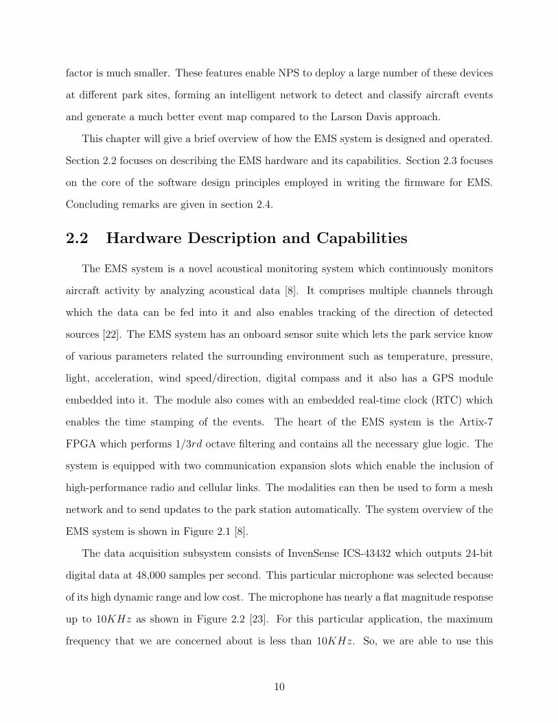
2.5 Conclusion
EMS system is a powerful extension to the existing acoustical monitoring technology
which typically uses expensive sound meters and microphones. The features that are present
in the EMS make it possible to perform onboard detection and classification without any
human intervention. The currently used Larson Davis method requires deploying the system
in a remote area and then retrieve it to manually process the 1/3rd octave data. This is done
by an expert using visual evaluation of the 1/3rd octave spectral data and then classifying
the sources of interest. EMS system, on the other hand, automatically records the acoustic
data, performs 1/3rd octave decomposition, detects and classifies the sources, and wirelessly
reports the events every few hours. EMS system can be used to form a mesh network and
work with other nodes for more accurate generation of noise map in national parks. However,
when using a large number of EMS nodes, there are practical issues such as routing latency,
packet losses and excessive flooding of packets that are bound to happen especially when the
source to destination path is longer than one hop. These considerations limit the number of
XBee nodes to a few hundred in order to maintain a reliable operation.
It must be pointed out that in comparison to the Larson Davis system the 1/3rd octave
filter on the EMS uses a bank of digital filters as opposed to analog filters which don’t suffer
from quantization problems. However, the SCST algorithm works on sparsely coded and
quantized data [17], hence these quantization effects may have little impact on the final
detection and classification results. The application of EMS need not be limited to just the
detection and classification of airborne vehicles. The hardware and software of the FPGA
core can be reconfigured for different applications including: a) detection, classification, and
tracking of ground vehicles for surveillance, traffic monitoring, and border control; b) gun-
shot detection and location finding for both indoor and outdoor settings; c) detecting and
localizing poachers, etc.
24

CHAPTER 3
DESIGN AND ANALYSIS OF ONE-THIRD
OCTAVE FILTER BANK
3.1 Introduction
The purpose of the one-third (1/3rd) Octave filter implementation is to be able to gen-
erate 1/3rd spectral sub-band sound data on the EMS system. The data that is generated
from the filter bank module is then used by the onboard processing system (MicroBlaze) to
make detection and classification decisions. A spectral band is said to be an octave when
the highest frequency of the sub-band is twice the value of the lowest frequency in that
sub-band. Similarly, a spectrum is said to be a 1/3rd octave spectrum when the upper-edge
frequency in the sub-band is equal to lower-edge frequency times the cubed root of 2 [28].
For the purposes of this application, the iterative filter bank [20] implemented on the EMS
board splits the entire audio spectrum into 33 frequency bands or 11-octave bands where
each octave band has three sub-band frequencies or 1/3rd octave frequencies. The 1/3rd
octave filters have been implemented on the ARTIX-7 FPGA as a custom hardware unit so
that the full advantage of computational parallelism that is available on the FPGA can be
exploited.The filters that are designed meet the ANSI.S11 standards and are IEC class 0
compliant [28]- [29] . The implemented filters are 8th order digital infinite impulse response
(IIR) Butterworth filters, which are obtained by cascading four second order IIR sections.
This chapter aims to provide a description of the design strategies employed in the imple-
mentation of the 1/3rd octave filter bank explained in Section 3.2. In Section 3.3 effects of
quantization have been analyzed for the Direct Form II implementation of the 1/3rd octave
filter bank. Section 3.4 discusses some of the issues related to the quantization noise in the
25

upper band filters associated with the Direct Form II structure and ways to correct it by
using a Lattice-Ladder implementation of the 1/3rd octave filter bank.
3.2 Iterative 1/3rd Octave Filter Bank Implementation
- An Overview
In an ideal situation, in order to split the spectrum into 33 sub-bands, we would need
to apply 33 filtering operations. However, to reduce the number of resources needed for the
implementation, the specification has been achieved iteratively by making use of only one
second-order Direct Form II (DF II) IIR Butterworth filter. The iterating effect is achieved
by cascading four second-order sections (SOS) to achieve a 8th order filter. The other 1/3rd
octave frequency components in the octave spectrum are then obtained by just switching
the coefficients of the same filter by the use of a finite state machine. From the properties
of multirate systems, it is known that, downsampling a signal by a factor of N in the time
domain, stretches its spectrum in the frequency domain by a factor of N. The higher frequency
components present in the downsampled signal are aliased and need to be removed through
low-pass filtering prior to processing it in the filter bank. Hence, by just downsampling the
data by a factor of two for up to 11 times during successive iterations, one is able to sweep
through the whole audio spectrum and split it into 33 sub-bands. The multi-rate filter bank
architecture that is used to achieve this functionality is shown in Figure 3.1. In this figure,
SOS corresponding to the first row is associated with the anti-aliasing low-pass filter, the
second row corresponds to the band-pass filter in the upper band, the third row corresponds
to the band-pass filter in the middle band and the fourth row corresponds to the band-pass
filter in the lower band. Each row in the Figure 3.1 has four SOS’s, implementing an 8th
order filter. The sampling rate switching is controlled by a finite state machine in the code,
which also handles the switching of coefficients to extract the samples in the upper band,
the middle band, and the lower band, respectively. The sampling rate is initially set to the
highest value of 50kHz and once the filtering is done in the higher, middle and lower bands
26

at the highest sampling rate, the state machine then downsamples the input and then the
input is bandlimited by using a low-pass filter to remove the aliasing effects which occur due
to downsampling and the process is repeated. The Multi-rate Timing block shown in the
Figure 3.1 contains the logic for filter selection by sending the appropriate select line bits
to the multiplexer module and also the logic for sampling rate reduction. The Multi-rate
Timing block implements 11 rates in total, and at each rate, the input is downsampled by a
factor of 2.
Figure 3.1: Multi-rate Filter Bank Architecture.
Figure 3.2 shows the time interleaving scheme employed in the 1/3rd octave filter bank
design [20]. Each colored box represents one-time step. Since the filters are operating at a
frequency of 50kHz, each time step is 20µs. The marked box indicates that the corresponding
octave was executed during that time step. It can be noted from Figure 3.2 that the highest
octave bands are executed in every time step, the second highest octave in every two time
steps, the third highest octave in every four time steps, the fourth highest octave in every 8
time steps, and so on. Hence, the last octave or the 11th highest octave which corresponds
to the lowest sampling rate is executed every 210 time steps. It can also be noted that during
each time step two octave bands or six 1/3rd octave bands are computed. The Multi-rate
Timer block in Figure 3.1 first also decides the octave that needs to be executed during each
27

time step and then executes the filters corresponding to those octaves. The upper, middle
and lower band associated band-pass filters within each octave are executed by choosing the
appropriate coefficient inputs. The choice of switching the coefficients is made by keeping
track of the number of clock cycles. This is done in VHDL by tracking this information in a
counter array which is 4 bits wide and 6 bits deep. The reason why this array is 4 bit wide
is that the first two bits keeps track of the individual second-order section (four) while the
last two bits keep track of the number of stages in each 1/3rd octave band (four). The four
stages in each 1/3rd octave band are the three band-pass filters corresponding to the upper,
middle, lower sub-bands in that octave and the fourth stage corresponds to the anti-aliasing
low-pass filter. The counter array is 6 bits deep to account for the fact that, during each
time step, six 1/3rd octave filters or two-octave filters are executed.
Figure 3.2: Timing Interleaving Scheme.
The Direct Form II implementation of a single section is shown in the Figure 3.3. The
current Direct Form II implementation has only 3 multipliers, 4 adders, 2 delay blocks and
there is one multiplier to account for the gain factor. The filter coefficients of the Direct
Form II filter are 35 bit wide. The reason for choosing 35 bits is to reduce the coefficient
quantization effects. It can also be noted that the Direct Form II filter structure uses the
smallest number of delay blocks which makes it the most suitable filter structure to be
implemented on the FPGA because of its inherent low memory requirements. The transfer
28

function for the low-pass and the band-pass filters for each type is represented by,
H(z) =4∏
k=1
Hk(z) (3.1)
where Hk(z) is given by,
Hk(z) =4∏
k=1
(b0k + b1kz
−1 + b2kz−2
1 + a1kz−1 + a2kz−2) (3.2)
where a1k, a2k, b1k and b2k are the filter coefficients for the low-pass and the band-pass filters.
The filter coefficients A1, A2, B1, B2 in Figure 3.3 are related to those in (3.2), i.e.: a1k = A1,
a2k = A2, b0k = G, b1k = B1G, and b2k = B2G, respectively.
Figure 3.3: DF II Second Order Section.
The two delay blocks shown in Figure 3.3 are implemented in the FPGA by designing
two 256 bit RAM modules with an 8-bit addressing scheme. As stated previously, the 1/3rd
octave filter bank computes 6 1/3rd octave time step. Hence, the RAM needs to be able to
buffer six samples of data, with each sample being 35-bits. This is the reason why the RAM
was designed to have 256 bits of memory. The delay elements are stored in this RAM by
explicitly specifying a write address and this write address is a function of the current sam-
pling rate, the filtering stage, and the current computational stage, where rate corresponds
29

to the sampling rate currently being used. The computational stage array explicitly keeps
track of each filtering stage which corresponds to the band-pass filters in the upper, middle,
lower sub-bands and the low-pass filtering stage. The computational stage is kept track of
by using an array which is 6 bits deep and 2 bits wide. The reason for using 6 bits is that
the FPGA computes the filtered output for 6 1/3rd octave segments per time step. The 2
bits in each row of the array keeps track of all the four stages that are available in the filter
bank. The filtering stage component is also an array that is 6 bits deep and 2bits wide.
The filtering array keeps track of each individual second-order section in the band-pass filter
modules of the 1/3rd octave filter bank. All the band-pass filters and also the anti-aliasing
low-pass filter has four SOS associated with it and all the four second order sections can
be tracked from the two bits that are available in the filter array. The computational stage
array and the filter stage both ultimately functions of the number of clock cycles and these
arrays are updated by using the counter array by referencing the appropriate bits and rows
from the counter array. The information pertaining to the first two bits of every row in the
count array is associated with the completion of each SOS and the last two bits are associ-
ated with each stage present in the octave band. A write address for the RAM is generated
by concatenating the values of current rate and the appropriate bits in the filter array and
the computational stage array. The read address for the RAM is also generated in a similar
fashion by tracking the same components. The operation of coefficient switching is also
performed by tracking the filter array and the computational stage array. The 3 coefficients
A1, A2, B1 and the gain factor G (from low pass filtering) of the Direct Form II filter shown
in the Figure 3.3 are stored in the form of a 4 × 4 array and the fourth coefficient B2 is
hardcoded to unity. The coefficients are changed by indexing into these coefficient arrays by
using the filter array and the computational stage arrays which ultimately are functions of
the number of clock cycles occurred since a new sample was received. The first three rows in
the coefficient array are associated with one of the upper, middle, lower band-pass filters of
the 1/3rd octave sub-band, while the fourth row is associated with the anti-aliasing low-pass
30

filter. As an example, the coefficient array for the B1 coefficient in Figure 3.3 is expressed as,
2 2 2 2
2 2 −2 −2
2 2 −2 −2
2 2 −2 −2
Figure 3.4 shows the generalized magnitude response of three band-pass filters. The
normalized center frequencies associated with the upper band, middle-band and the lower
band are 0.78π, 0.625π and 0.488π, respectively. Depending on the sampling rate, the actual
value of these center frequencies will change for each octave.
Figure 3.4: Magnitude Response of the 1/3rd Octave Filter Bank.
Once the filtering is performed for each of the 33 sub-bands in the 1/3rd octave spectrum,
a valid bit associated with each of those is set to high. Since there are 33 sub-bands, a 33-bit
wide register vector is maintained to keep track of the valid bits for all the sub-bands. The
filter module produces raw output samples, each of which are represented by 35 bit wide
fixed-point numbers. The filter output is then converted to 32-bit floating point format to
obtain higher precision before energy is calculated for each of the 33 sub-bands in every one-
second interval. Once the energy is computed, it is then converted to Sound Pressure Level
31

and expressed in dB (SPLdB). Note that the Effective Input Noise (EIN) of the microphone
is subtracted from the energy value before it is converted to dB. This process is repeated
across all the 33 sub-bands and for each sub-band and there is a valid bit associated with
every calculated energy level. A 33-bit wide register vector is maintained to keep track of
the valid bits for all the energy levels. Once all these valid bits are set to 1, the 1/3rd octave
filter bank generates an interrupt to the MicroBlaze processor, which typically occurs once
every second.
3.3 Quantization Error Analysis of DFII Structure
Here, we only consider the effects of product quantization since this is the most dominant
source of error in digital filters. Additionally, the effects of coefficient quantization are almost
insignificant and don’t alter the location of poles and zeros of the transfer function enough to
distort the frequency response of the system. This can be verified from the pole-zero location
plots in Figures 3.5a, 3.5b, 3.5c for DFII-based IIR Butterworth digital filters and using a
coefficient word length of 35 bits . The locations for the quantized and non-quantized pole
locations are marked by ’+’ and ’*’ in these figures and it can be seen that they are nearly
at the same spot in the unit circle. All the filter coefficients for this system were designed
using fixed-point arithmetic instead of floating-point arithmetic as floating-point operations
are computationally expensive. An analysis was done by designing the 1/3rd octave filter
bank at various coefficient word lengths and it was found that 35 bits is the optimum word
length at which the system produces a frequency response with minimal deviation from the
ideal non-quantized version.
32

(a) Upper Band-Pass Filters.
(b) Middle Band-pass Filters.
(c) Lower Band-pass Filters.
Figure 3.5: Pole-Zero plots for DFII Structure.
33

As mentioned before, the Larson Davis system uses analog filters and hence, do not suf-
fer from quantization effects. As a result, we can use the 1/3rd octave spectrum generated
by Larson Davis as a basis of comparison to analyze how much the 1/3rd octave spectrum
generated by EMS is distorted due to the effects of quantization. A test was conducted in
an abandoned airport in Fort Collins where a chirp signal from 250Hz to 2kHz was played
through the speakers while both EMS and Larson Davis were placed approximately in the
same location. The collected 1/3rd octave data is used to generate time-frequency plots for
EMS and Larson Davis as shown in Figures 3.6a and 3.6b, respectively. As can be clearly
seen, the Larson Davis system produced clean 1/3rd octave data while the data produced
by EMS is slightly distorted since the energy values actually leak into adjacent frequency
bands. As can be seen, the leaking effect is more pronounced in the higher frequency bands.
This may be attributed to aliasing effects due to the folding of the spectrum caused by
downsampling and the imperfections of the anti-aliasing low-pass filter which does not com-
pletely remove these effects. If this leaking effect becomes more prominent, the detection
and classification accuracy could potentially suffer, despite the fact that the SCST algorithm
uses quantized data after sparse coding to perform detection and classification.
Product quantization is observed at the output of every multiplier module in the digital
filter. The outputs of these multipliers are used to generate a sum of the signal and the
quantization error at each adder output. Product quantization is usually the most prominent
type of quantization error. This is because, when two numbers each with a word length of
B bits are multiplied, together the product could yield 2B − 1 bit result. But in order
to maintain a constant word length of B bits, the B − 1 LSB bits have to be truncated
or rounded-off. This process can result in serious quantization errors, which is especially
prominent for IIR systems because of the recursive nature. For a multiplier with coefficient
bi and input x(n), the product quantization error e(n) is defined as,
e(n) = bix(n)−Q[bix(n)] (3.3)
34

(a) EMS System. (b) Larson Davis.
Figure 3.6: Time-Frequency 1/3rd Octave Plots for both Systems.
where Q[.] stands for the quantization process.
It can be easily verified [30] that the mean and the variance of e(n) for round-off error
are,
µe = E[e(n)] = 0 (3.4)
σ2
e = E[e(n)2] = (2−2B)/12 (3.5)
where E[.] is the expectation operation.
It is also known that for a Direct Form II filter, the round-off noise power spectrum is
given by,
Sff (ejΩ) = σ2
e |Hef (ejΩ)|2 + 2πµ2
fδ(Ω) (3.6)
where Hef (ejΩ) is the frequency response of the filter and µf is the mean at zero frequency
given by,
µf = µeHef (ej0) (3.7)
35

Round-off error analysis is performed using DSP toolbox in MATLAB which uses (3.6) for
Direct Form II filter implementation using structure used in the filter design to generate a
round-off noise power spectrum. The noise power values observed at the center frequencies
of the associated power spectrum at each sampling rate are used to form the basis of analysis
in this chapter.
Figure 3.7 shows the plots of the upper band, middle band and lower band frequency
filters and their round-off noise power spectrum values in dB at various sampling rates. It
can be seen from this figure that the upper band filters are more susceptible to round-off
noise compared to the lower ones. This can be due to imperfections in the anti-aliasing
low-pass filter that are used to remove high frequency aliased components resulted from
downsampling. The other reason could stem from the fact that the microphone only produces
24-bit samples which might not provide enough resolution to accurately capture the data.
Another observation that can be made is that, as the sampling rate reduces, the round-off
noise power values increase. It was seen from the Figure 3.2 that as the sampling rate reduces,
the lower octaves are executed a smaller number of times compared to higher ones. That is,
we have a smaller number of samples adding up to one second, thus it may not provide an
accurate average power. Thus, the lowest center frequencies are the most affected ones.
Figure 3.7: Direct Form II Quantization Effects in all the three filters.
36

3.4 Quantization Error Analysis of Lattice-Ladder
Structure
It is clear from the analysis presented in Section 3.3 that at certain frequencies (20Hz
and 40Hz) the quantization effects are very dominant, though the sources of interest do not
lie in this frequency range. It must be pointed out that for the test results shown in Figures
3.6a and 3.6b, the lowest frequency considered was 250Hz, and the round-off noise at this
frequency was −145dB which is fairly low and does not degrade the SNR enough to cause
any detection and classification issues. The question is: Is it possible to improve the overall
SNR of the 1/3rd octave spectrum and decrease the quantization effects considerably so that
the EMS can operate nearly as good as the Larson Davis?. The answer to this question is
yes, and the solution is Lattice−Ladder architectures [31]. Prior research [32] shows that for
fixed-point IIR filter implementation, the stability and frequency response of Lattice-Ladder
structures are less prone to round-off errors. This would mean that we can implement the
same filter bank with coefficients of smaller word length without causing significant round-off
errors. Lattice-ladder structures are also shown [33] to have fewer limit cycle oscillations as
compared to classical implementations. In this thesis, the Butterworth filter coefficients that
were originally computed for the Direct Form II structure have been reconfigured to fit the
lattice-ladder structure by using filter convert method readily available in MATLAB’s DSP
toolbox. This is done to make sure that our comparison is consistent and we can attribute
the change in behavior solely to the filter structure and not any to any other design changes.
Figure 3.8 shows lattice-Ladder implementation of the same 1/3rd octave filter bank .
Note that this figure only shows a part of the complete implementation (3 sections) out of the
8 sections for 8th order filter implementations. The word length of the filter coefficients in
this implementation is chosen to be 24-bits as opposed to 35-bits in the case of Direct Form
II considered before. Figure 3.9 shows the magnitude responses of the three band-pass filters
for the lattice-ladder implementation of the 1/3rd octave filter bank. As can be seen from
Figures 3.4 and 3.9, even at 24-bit coefficient quantization, the lattice- ladder architecture
37

Figure 3.8: Lattice-Ladder Filter Architecture.
exhibits similar magnitude responses compared to the DF II implementation with 35-bit
coefficient word length.
Figure 3.9: Magnitude Response of Lattice-Ladder Implementation.
For the sake of consistency, a similar quantization error analysis was done for the lattice-
ladder filter realization by computing the round-off noise power at all the 11 sampling rates in
order to compare the results with those of the 35-bit DF II implementation as shown in Figure
3.10. More specifically, the performance of both filter architectures is benchmarked at higher
frequency bands with higher (for DFII) round-off error issue. Figure 3.11 gives a plot of the
38

noise power versus frequency, evaluated at higher frequency bands for both DFII and Lattice-
ladder realizations. From these results, it is evident that the lattice-ladder implementation
performs better and is much less susceptible to the quantization errors at these frequency
bands. The noise power value at 20Hz and 40Hz for lattice-ladder architecture is −60dB
which reveals a significant improvement over Direct Form II-based implementation.
Figure 3.10: Lattice-Ladder realization Quantization Effects for all the Three Filters.
Figure 3.11: Lattice-Ladder implementation vs DF II implementation-Upper band Quanti-zation.
39

3.5 Implementation Considerations for Lattice-ladder
vs DFII
Group Delay: While the magnitude response of a filter gives the information about the
signal output strength across the various frequencies, the phase component gives a way to
measure the signal distortion that is, the rate of change of phase. Group delay, τ , is defined
as the rate of change of phase, φ, with respect to the frequency, ω, which gives a measure of
signal distortion,
τ = −∂φ/∂ω (3.8)
From Figures 3.5 and 3.13 we can see that the poles for both realizations are located at
approximately same locations, while in case of DF II realization the zeros are located on the
unit circle, so opposed to the zeros of Lattice Ladder implementation which are scattered
all over the z-plane. This implies that both systems are essentially non-minimum phase
systems. Hence, the group delay for both systems would not be minimized. Nevertheless,
it can be noticed from Figures 3.12a and 3.12b that the group delay of the lattice-ladder
architecture is about a few tens of microseconds versus that of the for Direct Form II which
turns out to be a few tens of milliseconds. Moreover, the group delay in DF II realization is
not constant for all frequency components as opposed to the lattice-ladder realization which
exhibits a nearly constant group delay at all frequencies. A non-constant group delay usually
translates to signal distortion. This might explain why the EMS system could not produce
1/3rd octave data as accurately as the Larson Davis system (refer to Figure 3.6).
40

(a) DF II Implementation.
(b) Lattice-Ladder Implementation.
Figure 3.12: Group Delay for both Filter Implementations.
Hardware Implementation Complexity and Resource Consumption: When de-
signing filters on the custom system on chips such as FPGAs, it is usually a standard
practice to go with the DF II structure with cascaded SOS’s when it comes to IIR filter
design. Moreover, implementing DFII filter on the hardware through RTL coding is fairly
straightforward and simple. The main reason is that it is easily scalable to higher orders
while keeping the resource requirements constant. Whereas, lattice-ladder implementation is
significantly more complex to code if we do not break the filter into sections and modularize
it. The caveat here is that we need to accurately know what poles and zeros to pair up when
we modularize lattice structure to make sure that the frequency response is not distorted
41

(a) Upper Band-Pass Filters.
(b) Middle Band-pass Filters.
(c) Lower Band-pass Filters.
Figure 3.13: Pole-Zero Plots for Lattice-Ladder Structure.
42

and the stability is not compromised. This is actually a laborious process. Referring to Fig-
ures 3.13a, 3.13b, 3.13c, it can be seen that this could be a challenging problem to properly
accomplish for all the octaves in our hardware as the zeros are scattered all over the z-plane.
Table 3.1: Implementation Cost in terms of Resources for 8th Order IIR Filter
Filter Structure Number of Adders Number of Multipliers Number of Delay BlocksDF II 4 43 2Lattice-Ladder 23 24 8
Additionally, lattice-ladder realizations inherently consume more resources than other
traditional forms of filter realizations on the FPGA [32]. From Table 3.1 it can be seen that
for 8th order filter implementation, lattice-ladder filter uses a significantly higher amount of
resources compared to DFII realization, which can pose scalability issues. Higher resource
utilization usually translates to higher power dissipation and this can be undesirable in
battery operated sensor nodes.
3.6 Conclusion
The 1/3rd octave filter bank implemented on the EMS system is highly resource efficient
and capable of achieving high sampling rates. The filter bank is designed in such a way that
the filter order can be scaled without causing significant hardware overhead. The analysis of
quantization effects of the DF II filter structure indicated that the upper-frequency band-pass
filters were more susceptible to quantization errors compared to other frequency bands. We
also verified numerically that a lattice-ladder implementation of the 1/3rd octave filter led
to less susceptibility to quantization effects compared to the DF II filter structure. However,
was also noted that implementing a lattice-ladder filter bank is significantly more complex
compared to the implementation of DF II on the FPGA. The higher amount of resource
consumption and hence, higher power requirement makes it unsuitable for FPGA based
environments. Moreover, as discussed in Section 3.3 the center frequencies that are more
susceptible to quantization noise are 20Hz and 40Hz. But, the acoustic signature produced
43

by the sources of interest is usually higher than 100Hz and any signal below this frequency
is usually treated as interference and canceled out by the SCST algorithm. Thus, this issue
is not likely to affect our detection and classification results.
44

CHAPTER 4
EMS COMMUNICATION SYSTEMS
4.1 Introduction
As mentioned in Section 2.2.1 one of the main features of the EMS system is its ability
to autonomously report the classified events to the park station. EMS system is designed
with two expansion slots: one for a cellular module and another for an XBee transceiver.
This flexibility allows the EMS systems to use either the GSM module or the XBee radio
and transmit data to a park station depending on the availability of cellular service in the
deployment location and the distance between the deployment sites and the park station. It
is important to note that only a few EMS nodes, known as the master nodes, will need to be
facilitated with the GSM feature, whereas all the EMS nodes will have XBee communication
facility. The nodes that only have XBee’s mounted on them are referred to as slave nodes.
The master modules act as gateways in the network. This communication scheme allows
slave nodes to be deployed in areas with poor cellular connectivity so long as they are able
to communicate to adjacent nodes using the XBee radios and route their data to a master
node which has good cellular connectivity. The EMS Xilinx Artix 7(XC7100T)-based main
board populated with the GSM and XBee expansion prototypes were shown in Figure 2.5.
This chapter focuses mainly on the design and analysis of the communication system for
the EMS board. Section 4.2 focuses on addressing some of the terminologies related to the
Zigbee protocol and Zigbee communication as applied to the EMS system. In Section 4.3
a mesh network consisting of six EMS nodes is simulated and an analysis is presented to
evaluate packet losses in the network as a function of the distance between the nodes and
also as a function of a node failure within the network.
45

Section 4.4 describes how the data is transmitted to the park station using the GSM
module. Conclusions are presented in Section 4.5.
4.2 Zigbee Communication
XBee is a brand name for Zigbee’s developed by Digi International. Xbee PRO is a high
power version of the XBee which comes with a much higher transmission range and receiver
sensitivity in comparison to standard XBee. The XBee module currently being employed in
the EMS system is the XBee PRO S3B paired up with a 2.1 dBi (decibel with respect to
isotropic) half wave dipole antenna [34].
Zigbee protocol can be understood by reviewing its four important layers : a) Physical
layer (PHY), b) Media Access Control layer (MAC), c) Network layer and d) Application
Layer as shown in Figure 4.1. The PHY and the MAC layers of the Zigbee are defined by the
IEEE 802.15.4 Wireless Personal Area Network (WPAN) standards [35] while the Network
and the Application layers are defined by the Zigbee Alliance [36]. IEEE 802.15.4 WPAN
standards define two PHY layer formats, one for modules operating at 2.4GHz and the
other for modules operating at 868/915MHz. The 868MHz band is allowed only in Europe
while the 915MHz band is allowed in the North American region for radio communication.
From the literature it is known [37]- [38] that the path loss is proportional to the logarithmic
inverse of wavelength. The modules operating in the 868/915MHz have more than twice
the transmission range in comparison to the modules operating at 2.4GHz [38]. Hence, a
Zigbee module which operates at 915MHz frequency was specifically chosen for EMS appli-
cation. At the MAC layer, Zigbee uses Carrier Sense Multiple Access protocol with Collision
Avoidance feature (CSMA/CA). In the CSMA/CA protocol, the packet transmission to the
destination node is only performed when the communication channel is available. If the com-
munication channel is occupied, the transmitter holds the packet for a random time frame
defined as the backoff factor which is basically a down counter that has a pre-set maxima.
The transmission channel is checked again after the backoff counter gets to zero and if the
46

channel is free, the packet is transmitted or else the backoff factor is re-adjusted and the
whole scenario is repeated again until the channel becomes available. Once the packet is
transmitted, the source looks for an acknowledgment from the receiver by waiting for a short
time frame known as the receiver timeout. If the acknowledgment is not received within
this time frame, the packet is assumed to be lost and a re-transmission is set up. It is to be
noted that the transmission process will be initiated only if the destination node is within
the transmission range of the source. Moreover, the Collision Avoidance (CA) feature of
the MAC layer ensures that no two valid packets of the 802.15.4 format [39] are transmitted
simultaneously to the same receiver. The transmission range at the MAC layer is defined
by a factor known as Receiver Sensitivity [40]. Receiver sensitivity is defined as the lowest
power at which the signal is distinguishable from the noise. This information is provided by
the Zigbee manufacturer.
Figure 4.1: Zigbee Protocol Stack.
At the Network layer, Zigbee uses a routing protocol known as Ad-HOC On-Demand
Distance Vector (AODV) [41]. In this protocol, the source to destination path is not fixed
and the path is dynamically allocated during each transmission through a process known
as route discovery. In this networking scheme, a routing table is maintained at every node
that records all possible active paths from source to destination and also flags the nodes
that are part of the active connection. The routing table also stores information about the
destination address, next hop address, sequence number and the lifetime of the route. If the
47
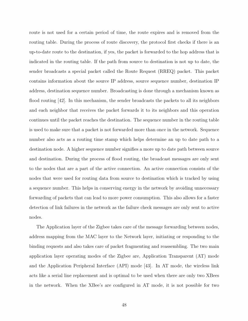
route is not used for a certain period of time, the route expires and is removed from the
routing table. During the process of route discovery, the protocol first checks if there is an
up-to-date route to the destination, if yes, the packet is forwarded to the hop address that is
indicated in the routing table. If the path from source to destination is not up to date, the
sender broadcasts a special packet called the Route Request (RREQ) packet. This packet
contains information about the source IP address, source sequence number, destination IP
address, destination sequence number. Broadcasting is done through a mechanism known as
flood routing [42]. In this mechanism, the sender broadcasts the packets to all its neighbors
and each neighbor that receives the packet forwards it to its neighbors and this operation
continues until the packet reaches the destination. The sequence number in the routing table
is used to make sure that a packet is not forwarded more than once in the network. Sequence
number also acts as a routing time stamp which helps determine an up to date path to a
destination node. A higher sequence number signifies a more up to date path between source
and destination. During the process of flood routing, the broadcast messages are only sent
to the nodes that are a part of the active connection. An active connection consists of the
nodes that were used for routing data from source to destination which is tracked by using
a sequence number. This helps in conserving energy in the network by avoiding unnecessary
forwarding of packets that can lead to more power consumption. This also allows for a faster
detection of link failures in the network as the failure check messages are only sent to active
nodes.
The Application layer of the Zigbee takes care of the message forwarding between nodes,
address mapping from the MAC layer to the Network layer, initiating or responding to the
binding requests and also takes care of packet fragmenting and reassembling. The two main
application layer operating modes of the Zigbee are, Application Transparent (AT) mode
and the Application Peripheral Interface (API) mode [43]. In AT mode, the wireless link
acts like a serial line replacement and is optimal to be used when there are only two XBees
in the network. When the XBee’s are configured in AT mode, it is not possible for two
48

sources to send packets to the same destination simultaneously. The sources are required
to be temporally synchronized in such way that the transmission overlap is avoided, which
otherwise, can lead to loss of information. Moreover, the destination node needs to be
re-configured before sending each packet, making it difficult to use AT mode in an XBee
network. On the other hand, API mode is specifically designed so that communication
between multiple nodes can be easily established without the worry of information loss. In
API mode, instead of directly sending raw serial data over the air, the data is sent in the
form of packets known as API frames. The frame consists of various fields as shown in
Figure 4.2. The start delimiter field consists of a predefined data sequence (0x7E) which
indicates the beginning of a data frame. The length field is used to denote the number
of bytes present in the frame data field. The frame data field consists of the 64 bit MAC
address of the destination device along with the actual payload. Lastly, the checksum field
is used to evaluate the data integrity. In API mode, the packet source address can be easily
identified as the received data includes the sender’s address, that can be used to pinpoint
node failures. Each received packet also contains the Receiver Signal Strength Index (RSSI)
value, which helps in evaluating link quality.
Figure 4.2: API Frame Packet Structure.
In the EMS system, the XBee is interfaced with the ARTIX-7 FPGA through a Universal
Asynchronous Receiver Transmitter (UART) bus. The UART is configured to operate in the
interrupt mode, which means that the processor will be stalled until the whole string of data
is transmitted or received through the UART. The interrupt handler for the XBee UART
consists of an event counter which counts up after each byte of data is processed by the
UART. The interrupt is not released until a pre-specified number of bytes of data has been
processed. The EMS system is configured to send the GPS coordinates, time stamps, the
49

sensor suite measurements, node ID and actual counts of the classified sources. The data is
packaged in the string format. The range of possible values for the length of this string was
experimentally determined to be between 120 to 128 bytes. The actual size of the string will
vary depending on the sensor outputs. Since it is hard to predict the actual size of the string,
the XBee UART is configured in such a way that it always sends and receives 128 bytes. If
the actual length of the string is less than 128 bytes, the string is simply zero-padded and
transmitted. This redundancy ensures that correct data is transmitted at all times. Since
XBee’s in the EMS are functional only a few times a day, the power consumed through
transmission and reception of data through XBee does not contribute to the average power
consumption of the board.
Figure 4.3: EMS Slave Node Operational Overview.
50

The operational overview of the communication systems of the slave module is shown in
Figure 4.3. The actual counts of the sources of interest are tracked using two counters that are
interfaced with the SCST algorithm in the MicroBlaze firmware. The current design reports
wirelessly to the park station once every few hours. This transmission event is controlled by
a timer interrupt that has been interfaced with the MicroBlaze softcore processor. Once the
interrupt is triggered, the GPS module is queried for Recommended Minimum Configuration
(RMC) data by sending a Proprietary MediaTek (PMTK) command to the GPS module
through serial UART bus, which is a transfer protocol for Global Navigation for Satellite
Systems (GNSS) designed by MediaTek. The queried RMC message contains information
related to the latitude, longitude, the time stamp of the coordinate lock, date, and speed
over the ground in knots. The obtained date and time information are used to initialize the
onboard real-time clock (RTC). The coin cell battery that is present in the EMS system, is
coupled with the RTC to make sure its values are always up to date , even when the board
is not powered. It can be noted from Figure 4.3 that, the reporting process is not initiated
unless GPS lock is obtained. This is because GPS is used to synchronize the RTC to get
accurate timestamps of the source events and this is very important for the beamforming
algorithm [22]. The softcore processor communicates with the IIC bus in parallel to read
the outputs from all the sensors, including the barometric pressure sensor, PCB temperature
sensor, accelerometer, 3-axis digital compass, light sensor and the battery gas gauge which
outputs the actual amount of charge in coulombs that is present in the battery. In the
SCST algorithm, two counters have been set up to keep a track of the number of events of
Jet and Helicopter classes . The collected data is then packaged into a string along with a
pre-specified node ID in a format that is compatible with the HTTP (Hyper Text Transfer
Protocol) post method and the PHP (Hypertext Preprocessor) application script that runs
on the server. Once, the XBee transmission is complete, the XBee UART interrupts are
disabled and the source counts are reset to zero. The timer interrupts are disabled and the
SCST algorithm will resume detection and classification.
51

4.3 XBee Mesh Network
At the time of writing this document, only two fully functional EMS nodes were built.
Thus, it was not possible to physically build a mesh network and instead, a network of
EMS nodes was built using a simulator to analyze packet losses as a function of the dis-
tance between the nodes. Additionally, intermediate node failure cases were introduced to
understand their impact on packet losses. Network Simulator-2 (NS-2) [44] simulator was
chosen to study the EMS network because of the substantial support it provides to simulate
802.15.4 modules and also due to its extensive use in literature to study wireless sensor net-
works. NS-2 is an open source simulator whose source code is written in C++. This allows
the user to easily modify the source code of the routing protocols to suit the specifics of the
system. NS-2 also allows the user to be very specific in defining the modeling parameters,
including the antenna details , radio propagation models, and network traffic details. The
simulator environment of NS-2 is based on Object-oriented Transaction command language
(OTcl) [44]. These features make NS-2 a perfect choice to study the EMS wireless sensor
network compared to other competitors.
In our simulation, a mesh network was constructed by considering six EMS nodes in the
NS-2 platform as shown in Figure 4.4 where nodes are classified as Coordinator, Routers,
and End device. This classification is done based upon the functionality of each node. The
coordinators and the routers in the network are fully functional devices (FFD), meaning, they
are able to transmit, receive and forward packets. The end device, on the other hand, is a
reduced functional device (RFD) which can only send and receive data but cannot forward
any packets. EMS end device, also known as the gateway, is equipped with both GSM and
XBee functionalities and acts as a gateway to the park station. The end device is mostly
asleep and only wakes up at certain times of the day to service other nodes in the network,
making it suitable to operate on battery for a longer period of time. In a XBee network,
there can only be one coordinator at any given time, which is responsible for initiating and
forming the network. The coordinator acts as a parent node to the router nodes that are a
52
part of the active connection from source to destination. A router node is also an FFD much
like the coordinator node, but it is mainly used to expand the network [45]. The routers are
also responsible for allowing new nodes to join the network.
Figure 4.4: A Mesh Network of Six EMS Nodes.
4.3.1 XBee Range Test
The purpose of this experiment was to understand how the packet losses vary as a function
of the distance between the nodes in the presence of interference and also to evaluate how
they would change when a node close to the gateway fails versus when a node far from the
gateway fails. In order to model the network as close to the real hardware as possible, the
range of the XBees used in the EMS system was first assessed in an environment consisting of
a fair amount of obstacles in the form of walls, trees, steel. The test was performed with two
XBee modules, by connecting one of the modules to the laptop using the Future Technology
Devices International (FTDI) XBee to USB adapter as shown in Figure 4.5. The other XBee
module was connected to the EMS board. The XBee connected to the EMS board acted as
the receiver while the XBee connected to the laptop was the sender. The data transmission
53

from the laptop to the EMS was set up by using XCTU software [46], provided by Digi
International.
Figure 4.5: XBee with FTDI Converter.
The two XBees were first pre-configured to operate in AT mode using XCTU. The test
configuration used in the XCTU software is shown in Figure 4.6. Cluster ID 0x12 was chosen
as the range type test, where the destination node echoes transmitted packets back to the
source as an indication of reception acknowledgment. Receiver (Rx) timeout is defined as
the maximum time in milliseconds the source waits to receive an acknowledgment. This
value is set as 1000 milliseconds. The Tx time is basically the time interval in milliseconds
between successive packets and this is set as 4000 milliseconds to allow for sufficient trials of
re-transmissions, in case of bad connectivity. The GUI in the XCTU software clearly displays
the RSSI values and the packet loss percentages. The test was carried out by placing the
two XBees 50m, 100m, 150m, 200m, 300m, 450m apart. The value of RSSI was noted down
at each of these cases and is plotted separately as a function of the distance between the
nodes in Figure 4.7.
It can be noted from Figure 4.6 that a packet was lost at an RSSI value of −60 dBm
(decibel milli-watt). By referencing Figure 4.7, it can be roughly estimated that packet
losses start occurring when the nodes are placed at 300 - 350m apart in a noisy environment
54

Figure 4.6: XBee Range Test Configuration.
constituting of trees, walls, ground etc. It must be noted that in this experiment, at each
proximity several RSSI values were obtained by aligning the Xbee’s at various angles other
than the line of sight and also by hiding one of the modules behind a tree or a wall to
induce shadowing effects. An average value of the RSSI measurements was then taken at
each proximity. The two-ray ground radio propagation model in the NS-2 simulator requires
the information about the receiver signal strength at all the node proximities to accurately
model the transmission range of the XBees. Hence, the RSSI values measured from this
experiment were used as a measure for range modeling in the simulator to create a more
practical scenario.
55

Figure 4.7: RSSI Variation with Distance.
4.3.2 XBee Mesh Network Simulation
The main purpose of this experiment was to understand the impact of router failures on
the packet transmission reliability when data is sent from the coordinator to the end device.
In this experiment, the source and the destination nodes were kept more than one hop
distance apart and the packets were forced to go through routers to reach the destination.
In a mesh network, there is often more than one path from source to destination, but this
will not be the case when some of the nodes in the network fail due to various reasons like
power loss or loss of line-of-sight. Hence, it is important to understand how the locations of
node failures affect the packet loss percentage in the network.
The simulation was executed by specifying the details shown in the Table 4.1. The an-
tenna that is coupled with the XBee PRO S3B module is a 2.1dBi half-wave dipole antenna,
which in linear scale translates to a transmission gain of 1.6. A half- wave dipole antenna is
an omnidirectional antenna, i.e., it has a spherical radiation pattern. The PHY and MAC
layers are defined by IEEE 802.15.4 standards as mentioned in Section 4.2.
The NS-2 simulator supports three radio propagation models, namely, the free space
model, the two ray ground reflection model, and the shadowing model. The free space and
56

Channel type WirelessChannelPHY Wirelessphy/802.15.4MAC 802.15.4Radio Propagation Model TwoRayGroundTwoRayGround System Loss factor 1Antenna Type OmnidirectionalAntenna gain 1.6Operating Band 915MHzData rate 40kbpsNumber of nodes 6Routing Protocol AODVMax Packet size (Bytes) 128Traffic Type constant bit rate (cbr)
Table 4.1: Modeling Parameters
the two-ray ground reflection models assume that the antenna’s radiation pattern is circular
in shape, whereas, the shadowing model assumes distorted radiation patterns (elliptical in
this case). The free space model assumes that there are no obstacles or interferences in the
path between source and destination. Free space model assumes the communication range
as a circle centered around the transmitter. If the nodes are within the circumference of the
circle, the nodes receive all the packets, if not, the nodes lose all the packets. The received
signal power Pr(d) in free space at a distance d is calculated by using Friis equation [47],
Pr(d) =PtGtGrλ
2
4π2d2L(4.1)
where Pt is the transmitted antenna power, Gr and Gt are the transmitter and receiver
antenna gains, respectively, λ is the wavelength of the RF carrier and L is the system loss
factor. It must be noted that a ground level sensor network will never satisfy a free space since
a significant fraction of the RF energy bounces off the ground, which results in reflection
losses. The closer the antennae are to the ground, the higher are the chances of ground
reflections and path loss. This can be understood by referring to the Okumura model [48]
57

for path loss, described by the equation
Pathloss ≈ Pr(d) + A(f, d)−G(htr)−G(hre). (4.2)
where, Pr(d) is the free space path loss, A(f, d) is the medium loss as a function of distance
and frequency, G(htr) and G(hre) are the gain due to the height of the transmitting and
receiving antenna from the ground.
The radio propagation model used in this experiment is the two-ray-ground reflection
model. This model considers both the reflected path and a direct path between the source
and the destination. Hence, this model gives a more accurate prediction of the link quality
between the nodes. When using the two ray ground reflection model, NS-2 calculates the
received signal strength PTRG(d) [47] as a function of distance d according to the following
equation,
PTRG(d) =PtGtGrh
2
th2
r
d4L(4.3)
where, Pt ,Gt and Gr were defined before, ht and hr are the heights of the transmitting
and the receiving antenna respectively. Here, the path loss factor L is assumed to be equal
to unity by default. The operating frequency band is set to 915MHz and the raw over
the air data rate corresponding to this frequency band is set to 40kbits per second. The
routing protocol, packet size, and the traffic type are set as indicated in Table 4.1. The
simulation was executed by placing the routers at 200m, 300m, 350m, and 450m apart. In
this experiment, the source (Node 0) and the destination (Node 3) were always placed more
than one hop distance apart as shown in Figure 4.4. This experiment is intended to evaluate
the effects of packet losses in the network based on the distance between router nodes and
based on node failure scenarios. The node failure cases were simulated in three separate
scenarios by causing a node close to the gateway to fail and a node far from the gateway
to fail. One more test case was also considered where one node close to the gateway and
another node far from the gateway fail simultaneously. This particular experiment was set
58

up such that Node 0 (coordinator) sends data to Node 3 (end device) while the other Nodes
act as routers. A constant bit rate traffic was set up between Node 0 and Node 3. Random
sized packets with a maximum allowed size of 128 bytes were sent continuously at a time
interval of 100 milliseconds between the packets and the simulation was run for a period of 20
seconds. Upon successful completion of the simulation, NS-2 simulator outputs a trace file
which contains the information about the number of packets generated, number of packets
dropped, number of packets received, number of packets sent and number of packets lost in
the network. The output trace file is then read into another tool called as tracegraph, which
helps in parsing the trace file and outputs the packet statistics as shown in Figure 4.8. The
packet loss percentage is calculated by using,
Packet Loss Percentage = (Number of Packets Lost x AveragePacket Size
Number of Bytes Sent) x100
(4.4)
Figure 4.8: Tracegraph Output Window.
In this experiment, the node failure cases were introduced by simply moving the nodes out
of the transmission range of all the other nodes. The node failure cases also were analyzed
by keeping the nodes apart at different distances away from each other. It is interesting
to note that the location of node failure also has an impact on the percentage of packets
lost. Figure 4.9 shows how the percentage of packet losses scale as a function of the distance
between the nodes when all nodes are healthy and also when there are node failures. It can
be noted that, when all nodes were healthy, packet losses don’t occur until 300m and there is
59

some packet loss observed when the nodes are placed at 350m apart. This is consistent with
the earlier test that was conducted to estimate the range of XBee’s in an environment that
was obstacle prone. As the distance between the adjacent nodes is increased, the percentage
of packet loss also increased. Another interesting fact that can be noted from Figure 4.9 is
that the percentage of packet losses are higher when a node close to the gateway fails as
opposed to the failure of a node far from the gateway. This is because, when node 2 fails,
during the process of flooding, Nodes 5 and 4 will try to flood the packets to Node 1, causing
the communication channel of Node 1 to be always busy. This results in more number of
re-transmissions and reception timeouts which ultimately translates to lost packets. The
situation becomes even worse when two routers fail in the network shown in Figure 4.9.
This happens because there is only one path from source to destination and in a ground
level sensor network scenario, it is highly probable that this path is obstacle prone which
decreases the effective transmission range.
Figure 4.9: Packet Loss Percentage as a Function of Distance.
60

4.4 GSM Communication
GSM functionality is exclusive only to the gateway in the EMS network. The GSM mod-
ule that is currently being employed is the UBLOX SARA-U260, which is a 3G module with
2G fallback compatibility. SARA-U260 supports High-Speed Packet Access (HSPA)/GSM
bands in North America [49]. High-Speed Packet Access (HSPA) is compliant with 3G tech-
nology while the Global System for Mobile Communication (GSM) is compliant with the
2G operating technology. SARA-U260 module can be coupled with T-Mobile and AT&T
sim cards in North America. The radio communication features supported by AT&T are
HSPA, High-Speed Uplink Packet Access (HSUPA) and High-Speed Downlink Packet Ac-
cess (HSDPA), in 3G operating mode, while also supporting LTE. T-Mobile, on the other
hand, supports GSM and Enhanced Data Rate for GSM Evolution (EDGE), both of them
being 2G operating modes. T-Mobile also has support for HSPA, HSUPA, HSDPA, and
Long Term Evolution (LTE). In addition, T-Mobile supports General Packet Radio Service
(GPRS) mode of communication, in which the network providers charge only for the amount
of data used and not for the duration of data used in this mode. GPRS is a packet-based
data service system that establishes communication with web applications through TCP/IP
sockets which can then be used to make HTTP (Hyper Text Transmission Protocol) POST
requests to the server. Additionally, HSPA and other LTE modes on the SARA U-260 mod-
ules are not optimized for power consumption. GPRS mode consumes less than a third
of the amount of power that is consumed in HSPA mode [49]. Since EMS only sends 128
bytes of data per transaction, it is unnecessary to operate the SARA-u260 module in the
high-speed HSPA or LTE modes. Hence, GPRS has been chosen as the preferred mode of
communication.
The SARA U-260 module is interfaced with the ARTIX-7 FPGA through a UART bus,
configured in the interrupt mode. Configuration and data transfer with the SARA-U260
module is done with the help of AT commands. Firstly, it is necessary to configure the
module with the appropriate Access Point Name (APN) , which is specific to the network
61

provider. The APN must be written into the nonvolatile memory of the SARA-U260 device,
before using it to send data to the park station. A GSM data transmission outlining the
following process is shown in Figure 4.10. Once data packets are received from the slave
module, the XBee interrupt lines are disabled and the GSM interrupt lines are enabled.
This is done to ensure that the GSM UARTS have full control over the MicroBlaze interrupt
lines until the data is transmitted. The configuration written in the non-volatile memory of
the GSM device is first read by the application layer of the GSM module. The GSM module
is then configured to communicate in GPRS mode. Next, a valid port number is assigned
to be able to send POST requests through TCP/IP sockets. The port number is set to 80
because the HTTP internet communication protocol uses Port 80 by default. HTTP POST
requests containing source counts, GPS coordinates, and sensor data are then sent to the
server application script that is written in PHP. As the server application receives the ASCII
data from the EMS board, data is parsed into variables. Single alphabetic letters are used
as parsing delimiters to reduce the amount of data sent per report. The variables are then
processed to convert them into appropriate units (SI) and stored in a MySQL (Structured
Query Language) database. The SQL database can then be queried to read each field and
plot the metrics on the website.
62
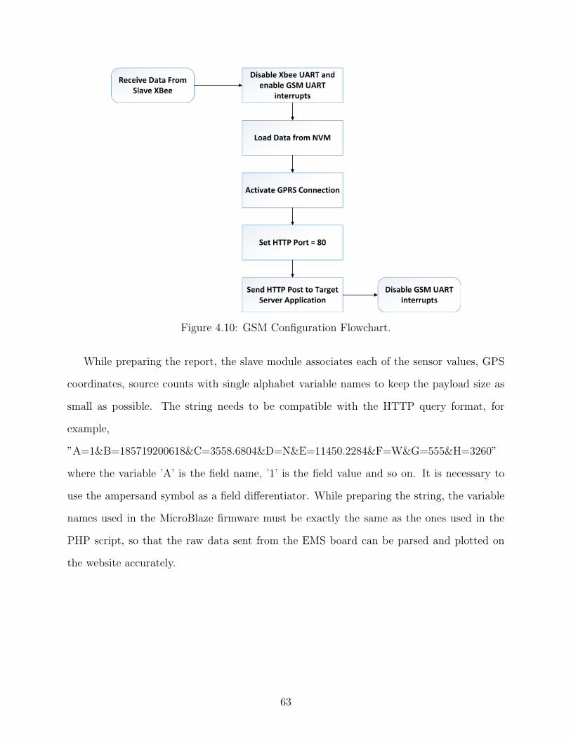
Figure 4.10: GSM Configuration Flowchart.
While preparing the report, the slave module associates each of the sensor values, GPS
coordinates, source counts with single alphabet variable names to keep the payload size as
small as possible. The string needs to be compatible with the HTTP query format, for
example,
”A=1&B=185719200618&C=3558.6804&D=N&E=11450.2284&F=W&G=555&H=3260”
where the variable ’A’ is the field name, ’1’ is the field value and so on. It is necessary to
use the ampersand symbol as a field differentiator. While preparing the string, the variable
names used in the MicroBlaze firmware must be exactly the same as the ones used in the
PHP script, so that the raw data sent from the EMS board can be parsed and plotted on
the website accurately.
63

Updating Detection Threshold Values through GSM: As mentioned previously,
the EMS system makes decisions using two detectors. The transient event detector looks for
the presence of sources under the assumption that none were previously present while the
quiescent detector looks for the spectral features that correspond to the end of the dominant
source event. The detection threshold values of these detectors need to be experimentally
determined and set before deploying the EMS system in the field. Currently, in the EMS
system, there is a provision to update these values from a remote location by sending text
messages to the GSM module as described in Figure 4.11.
Figure 4.11: Updating Detection Thresholds via SMS.
The GSM module is configured to accept text messages only from phone numbers that are
present in the approved list and text messages from other sources are deleted. The text
messages are configured to be stored in the SIM card memory to keep track of the received
64
messages in an orderly manner. As can be seen from Figure 4.11, the thresholds can be
updated either at power-on and/or once every few hours (whenever the EMS sends reports
to the web server). The approved user has to send the text message in the prescribed format
for example: ”S100” or ”s100” and ”N010” or ”n010” for updating transient and quiescent
detection thresholds, respectively. It must be noted that if the text messages are not in
the prescribed format, they will be discarded. The format, however, can be changed in the
future to suit the requirements.
4.5 Conclusion
The EMS system is designed to collect acoustic data, perform near real-time processing
on the data and send out periodic reports about the classified sources and the environmental
parameters. Every EMS node is equipped with a low power XBee transceiver, which allows
multiple EMS systems to be easily deployed in the form of an intelligent network in national
parks. As mentioned in this chapter, the XBee uses a process is known as route discovery
to dynamically estimate a routing path. That is, the EMS network can be designed to be
self-forming and self- healing, especially when there is more than one path from the source
to destination. This also indicates that new nodes can be easily added or the existing nodes
can be removed from the EMS sensor network without disturbing the functionalities of other
nodes. Ground reflections play a major role in reducing the transmission range of the XBee.
This issue can be minimized by mounting the XBee antennae on a high post to avoid these
reflections. An experiment was conducted to study the variation of the packet loss percentage
with respect to the location of the node failure. It was observed that more packets are lost
when a router node close to the gateway fails as opposed to the case where a router far
from the gateway fails. However, it is to be noted that, the environment where the data
was collected for the XBee range test consisted of interference from steel and various ground
automobiles such as cars, buses, etc. These sources of interference are unlikely to be present
deep within national parks. This would mean that, potentially, a better transmission range
65

can be expected from the XBee modules, provided the antennae are kept sufficiently off the
ground. EMS gateway is equipped with the GSM facility which is used to send data to a
park station. It has to be noted that the gateway must have good cellular connectivity at
all times to ensure the reports are reliably sent to the park station as there is currently no
efficient way to build redundancy into the system to deal with this issue. But as addressed
in Section 4.4, it is known that SARA-U260 module supports T-Mobile and AT&T carriers,
and these two network providers combined, provide sufficient coverage throughout out the
US. Hence, EMS, as it is, should be deployable in most national parks.
66

CHAPTER 5
FIELD TEST RESULTS
5.1 Introduction
Two EMS systems were recently deployed at the Lake Mead National Recreation Area,
where one system (slave) was deployed for the purposes of detection and classification, while
the other EMS system served as the master or gateway to the park station. The slave module
performed the detection and classification while also collecting the information about the
surrounding environment such as air pressure, temperature, etc and sent these reports to
the gateway wirelessly through the XBee link. The main function of the gateway was to
collect the data sent by the slave node through the XBee module and then hand over those
reports to the park station with the help of the onboard GSM module. The slave module
was first trained based upon annotated and labeled 1/3 octave data previously collected
over a 48-hour period (from 7/5/2016 to 7/7/2016) at Lake Mead National Recreation Area
(different physical location). The training involved building the dictionary matrices using the
K-SVD algorithm [18] for different source types and interference present at that particular
site and computing the log-likelihood values for each Bayesian network source model. These
dictionary matrices and log-likelihood values were then stored in the flash memory of the
EMS slave node. The system was specifically trained to detect and classify helicopters and
jets as these were the dominant sources of interest present at this particular site.
This chapter mainly focuses on analyzing the system performance and deployment limita-
tions using the results obtained during the recent field test conducted in Lake Mead National
Recreation Area. Section 5.2 focuses on explaining the experimental setup used in the field
test. Section 5.3 focuses on the analysis of the results and concluding remarks are presented
in Section 5.4.
67

5.2 Field Test Set Up
The trained system along with the gateway were deployed during June 20 to 21, 2018 in
Temple Bar Marina, located in the Lake Mead Recreational Area. The deployment location
was not the same as the one that was used to collect the training data. As a result, it was
important to re-evaluate the detection and quiescent threshold values before deploying the
systems to conduct a full system test.
As mentioned before, the detection and classification tasks on the EMS is done in two
phases: 1) signal detection to locate the presence of a transient signal of an unknown source
under the assumption that none were present and 2) quiescent detection to find the end
point of the transient signal by searching for observations where the particularly dominant
source is no longer present under the assumption that there was one present. Hence, the
EMS system was set up for a test run for an hour or so in the field to obtain the 1/3rd
octave data and also the log-likelihood ratios computed by the SCST algorithm, in the
presence of helicopter sources. The collected data was then plotted using MATLAB to
visually correlate the detection results corresponding to the generated 1/3rd octave spectral
images in order to set the right threshold values before the system was actually deployed.
These tests were conducted multiple times by re-configuring the EMS board each time with
quiescent threshold values namely, 5, 30, 50 while keeping the transient detection threshold
value at 100. The test conducted by keeping the quiescent detection threshold at γ = 10 and
the transient detection threshold at η = 100, yielded acceptable results for the helicopter
class. The high energy signatures shown by the yellow markings in the 1/3rd octave spectral
image in Figure 5.1a indicates the presence of helicopter sources. The quiescent and transient
threshold values are also displayed in Figures 5.1b and 5.1c. When the quiescent statistic of
a particular source type crosses the pre-set threshold (γ = 10), end of the source is declared
and the winning source is classified. As can be seen from Figures 5.1a, 5.1b and 5.1c, the
detection results correlate well visually with the 1/3rd octave data. Hence the EMS was
reconfigured with these quiescent and transient detection threshold values for this test.
68

(a) 1/3rd Octave Plot.
(b) Noise Log-likelihood ratio.
(c) Signal Log-likelihood ratio.
Figure 5.1: Detection and Classification Results.
To keep the EMS systems secure during the field test they were put in modified pelican
cases to ensure where the antennae are not enclosed within the case as shown in Figures 5.2b
69

(a) EMS slave node with microphone.
(b) Pelican Case architecture for Slave node. (c) Pelican Case architecture for Masternode.
Figure 5.2: EMS Field Deployment.
and 5.2c. The antennae of GSM and the GPS modules were connected to the case by using
suitable male-female SubMiniature Version A (SMA) extension cables and adapters, while
the XBee antenna was connected using reverse polarity SMA cables. The slave module was
connected to the digital microphone (Ivensense ICS-43432) and the time-series of the events
were recorded by using an audio recorder whose input lines were connected to an analog
microphone as shown in Figure 5.2a. The deployment set up for slave node along with the
microphones are shown in Figure 5.2a.
The test was conducted in a location which was exposed to a good amount of source
70
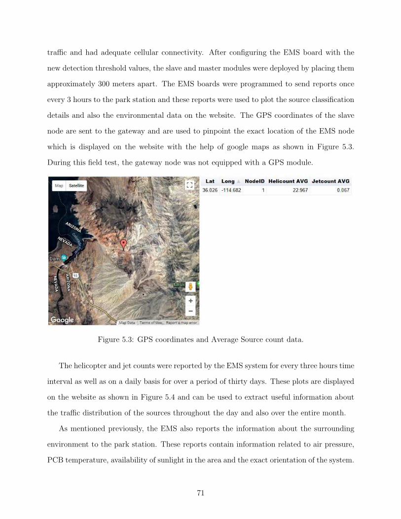
traffic and had adequate cellular connectivity. After configuring the EMS board with the
new detection threshold values, the slave and master modules were deployed by placing them
approximately 300 meters apart. The EMS boards were programmed to send reports once
every 3 hours to the park station and these reports were used to plot the source classification
details and also the environmental data on the website. The GPS coordinates of the slave
node are sent to the gateway and are used to pinpoint the exact location of the EMS node
which is displayed on the website with the help of google maps as shown in Figure 5.3.
During this field test, the gateway node was not equipped with a GPS module.
Figure 5.3: GPS coordinates and Average Source count data.
The helicopter and jet counts were reported by the EMS system for every three hours time
interval as well as on a daily basis for over a period of thirty days. These plots are displayed
on the website as shown in Figure 5.4 and can be used to extract useful information about
the traffic distribution of the sources throughout the day and also over the entire month.
As mentioned previously, the EMS also reports the information about the surrounding
environment to the park station. These reports contain information related to air pressure,
PCB temperature, availability of sunlight in the area and the exact orientation of the system.
71

Figure 5.4: Aircraft Counts Reported on the EMS Website.
The sensor data collected during the field test are also provided on the EMS website. For
the period of our tests, these plots that were generated and shown in Figures 5.5 - 5.9
correspond to 3-axis digital accelerometer, PCB temperature, air pressure, light sensor, and
3-axis digital compass, respectively.
It is important that the onboard electronic components always operate well within the
specified operating temperature range. During the field test, it was noticed that the PCB
temperature measured by the onboard sensor reached as high as 65 degree Celsius. It is
possible that the temperatures could get close to the operating temperature limit of some of
the onboard electronic components. It should also be noted that the Li-ion battery that was
used in this field test has an optimal temperature range from 0 - 45 Celsius. The battery life
and the charge acceptance will significantly reduce as the operating temperatures increase
beyond the optimal range [50]. The PCB temperature plots serve as an important tool
to monitor these factors and take appropriate actions to fix them. The light sensor data
72

shown in Figure 5.8 can be used for power management purposes by powering down some
non-essential systems when there is not much sunlight available to operate the system and
charge the battery. The 3-Axis digital compass data shown in Figure 5.9 can be used to
assess the precise orientation of the microphone array and the system in the beamforming
algorithm to estimate accurate Angle of Arrival (AoA) of the sources. This information was
not used in this study.
Figure 5.5: 3 Axis Digital Accelerometer Data.
Figure 5.6: PCB Temperature.
73

Figure 5.7: Absolute Barometric Air Pressure.
Figure 5.8: Light Sensor Data.
Figure 5.9: 3-Axis Digital Compass
5.3 Field Test Results and Observations
As shown in Section 5.2, the EMS system was able to perform detection and classification
of the sources, collect environmental data, and report all of this information automatically
to the park station. The detection and classification results in Figure 5.4 indicated that the
74

EMS system reported more than 600 helicopters while identifying only a few jet sources.
These results might suggest that there could have been quite a bit of misclassification of
the jet class. The helicopter sources occur more frequently compared to the jets because of
high traffic due to air tours at this particular park. Since the helicopters fly at a much lower
altitude compared to the jets, their acoustic signatures are also stronger (i.e, higher SNR).
There was also a significant amount of propeller plane traffic in the area and their acoustic
signature resembled very closely with those of the helicopter sources and could have led the
EMS system to misclassify them as helicopters. This is mainly due to the fact that the
training data for the system did not include any examples of the propeller plane sources [8].
Additionally, the training data was collected in a windy environment and labeling of this data
was performed by visual evaluation of the 1/3rd octave spectrum and also by listening to
the actual time-series data recorded during the system deployment. From the audio data, it
was evident that the acoustic signatures produced by the jet sources closely resembled strong
wind hence, causing misclassification and false alarms. Insufficient training data (imbalance)
pertaining to the jet class also indicates that the system was not trained well to identify all
cases of jet sources. Another key factor for classification error can be attributed to the fact
that the system was not deployed in the same location that was used to collect the training
data. This indicates that the SCST algorithm is not robust enough to a substantial variation
of location and needs to be trained on a larger set of data containing both helicopter and jet
sources to perform accurate detection and classification irrespective of where it is deployed
as the surrounding landscape has a huge impact on the captured acoustic signatures.
From the communication system standpoint, it was observed that the Lake Mead National
Recreational area does not have good cellular coverage in general, especially deeper within
the park. Even though there are a few cell phone towers present around the Lake Mead area,
the range of these towers is limited by terrain shielding caused due to the presence of hills
and mountains. It was observed during the field test that the cellular service in this area is
not reliable as the EMS system abruptly lost cellular connectivity for nearly nine hours and
75
had to be moved to a slightly different location before the tests were resumed again. Hence,
it is important to thoroughly investigate the location and make sure it has good cellular
coverage before deploying the system.
A range test similar to the one described in Section 4.3 was performed in the field be-
fore deploying the EMS systems. It was found that 300 meters separation between the slave
node and the master node was approximately the farthest distance that the slave and master
systems could be placed apart so that the no packets are lost at the time of XBee commu-
nication. At the time of this test, there was no provision to place the XBee antennae higher
above the ground and the terrain shielding in the vicinity made it harder to achieve a higher
transmission range for the XBee. The XBee PRO S3B module that was used during this test
has a line of sight range up to 9 miles [34], provided there is absolutely no RF interference
in the deployment region. Although it might not be possible to achieve this theoretical limit
in the field, the transmission range of the XBee modules can be improved by placing them
higher above the ground to avoid ground reflections as much as possible.
5.4 Conclusion
This chapter presented the results of our recent field test that was conducted in the Lake
Mead National Recreation Area. Two EMS systems were deployed in the field, where one
system was trained to perform detection and classification while the other system functioned
as a gateway. The detection threshold values were determined in the field by conducting
a test runs and visually evaluating the detection results collected during this test. Due
to insufficient training data available for the jet source class, it was noted that the system
wrongly classified a number of the jets as helicopters. The low detection threshold values may
have caused the system to perform classifications even before there was enough confidence to
make a decision. The detection and classification accuracy can be improved by re-training
the EMS system with a larger set of data and by more accurately determining the detection
threshold values by conducting multiple test runs in the field and verifying the onset and
76

endpoint of the detected sources as well as comparing the obtained classification results with
a truth table.
The EMS systems were, however, able to autonomously perform detection and classifi-
cation and send reports to a web server with the help of GSM and XBee modules. It was
noted in Section 5.3 that, the GSM module lost cellular connectivity abruptly during the
test. This was mainly due to the effects of terrain shielding in the deployment area. This
issue can be overcome by thoroughly investing the deployment area and making sure that
there is sufficient cellular connectivity before deploying the devices. It is also possible to
add another gateway in the network as a means of redundancy to account for this failure.
The transmission range of the XBee modules can be increased by placing the XBee antennae
within the line-of-sight and by keeping the antennae sufficiently off the ground to minimize
RF signal reflections.
77

CHAPTER 6
CONCLUSIONS AND SUGGESTIONS FOR
FUTURE WORK
6.1 Conclusions
The work in this thesis focused on the development of the communication systems and
their complete integration with the SCST algorithm and with the analog sensor suite on
the ARTIX-7 FPGA-based EMS system. A 1/3rd octave filter bank is implemented on the
FPGA to generate onboard near real-time spectral features of the captured acoustic signal.
The SCST algorithm implemented on the MicroBlaze softcore processor uses the output
of the 1/3rd octave filter bank to perform detection and classification tasks. The SCST
algorithm currently implemented on the EMS was specifically trained to detect and classify
the jet and helicopter sources. The classification results (source labels), along with the 1/3rd
octave data is stored in the SD card, while the source counts are tracked using a counter.
A fixed interval timer was implemented on the FPGA to time the reporting of the source
events.
The EMS node that performs detection and classification, transmits the results along
with the measured sensor data to a network gateway with the help of a XBee transceiver,
once every few hours. The EMS node that is equipped with the GSM module acts as a net-
work gateway and is responsible for posting the reports received from the other nodes onto
a web server. A full system test was conducted by deploying two EMS nodes in the Lake
Mead National Recreation Area during June 20-21, 2018. The EMS system was previously
trained for detection and classification on the data captured over 48 hours during July 5-7,
2016 in Lake Mead Area, though deployed in a different location at much higher elevation.
78

The detection thresholds were experimentally determined and adjusted in the field to accom-
modate for this change in ambient noise levels and signal strengths. It was found that the
EMS system frequently misclassified jets and propeller planes as helicopters. This is mainly
due to a lack of robust training data. Moreover, the training data did not contain examples
belonging to propeller plane class. Additionally, the acoustic signature of jets resembles that
of strong wind which makes the decision-making challenging especially when the training
dataset does not have enough samples of jets. It is also necessary to fine-tune some of the
parameters including the detection thresholds and the dictionary matrices to improve the
detection and classification performance of the algorithm.
As far as the communication systems are concerned, the XBee module was fully func-
tional and the slave system was able to send classification reports (source counters) along
with the measured sensor data to the master node (gateway) successfully. From the XBee
standpoint, it was noted that the farthest the two EMS modules could be placed apart was
approximately 300m to make sure that the packets were transmitted reliably at all times.
This limitation was mainly because the XBee antenna was placed close to the ground which
increased the likelihood of RF signal ground reflections, thereby reducing the effective trans-
mission range. Moreover, there was an intermittent problem related to cellular connectivity
in the deployment area. This issue can be addressed by thoroughly investigating the area
and making sure that there is good cellular coverage before deploying the EMS systems.
6.2 Future Work
Although EMS systems demonstrated autonomous detection, classification and reporting
of the source events, there is still some room for future work that needs to be done before
the EMS systems can be deployed as an acoustic wireless sensor network in the field.
79

Robust Training : It was observed, during the field test, that the SCST algorithm per-
formed many misclassifications. This is mainly due to lack of robust training data, particu-
larly for jet and propeller sources. The EMS systems need to be trained more thoroughly by
using a larger and more representative training data set for all source types present in the
particular site. It is desirable to collect the 1/3rd octave training data from various parts of
the national park to enable the SCST algorithm to accurately perform detection and clas-
sification independent of the deployment location. The detection threshold values also need
to be fine-tuned to make sure that interference signals do not get detected as sources.
Expert Evaluation: It is highly recommended that the detection and classification results
generated by the EMS be ground truth-ed by an expert from NPS to more accurately assess
the source of mis-detections and misclassifications. This evaluation can also help in coming
up with the right threshold values before the system is deployed in the field. It is possible
that most of the acoustic data captured in the field is affected by the terrain itself and this
factor needs to be accounted for while calculating energy values for the frequency sub-bands.
It would be valuable to work with experts at NPS to come with the right models that can
be incorporated in the firmware to cancel out this interference.
Network of Multiple Nodes : As mentioned before, we currently have only two fully
developed EMS systems and hence we were able to achieve automatic report generation from
a single node. This functionality needs to be expanded to multiple nodes to form a mesh
network of EMS systems. This work requires configuring the XBees in the API mode and
also changing the transmitting packet structure to API format as shown in Figure 4.2. The
MicroBlaze firmware for the gateway also needs to be changed by adding an array of buffers
to store the reports that are received from slave nodes to accommodate this feature. An
array of buffers should be added to store the reports that are received from the slave nodes
and data parsing code should be added to the gateway firmware as the received data will be
in API format, unlike the raw format in AT mode.
80

Enclosure Design : As mentioned in Chapter 5, the high ambient temperature in the Lake
Mead could pose a threat to the reliability of the onboard electronics. Hence, it is highly
desirable to conduct an industrial grade environment test on the EMS boards to pre-assess
their limitations during actual deployment. The EMS was enclosed within a pelican case as
shown in Figure 5.2 and this rules out the usage of the light sensor to assess the ambient
sunlight. This can make it challenging to asses when to use a battery and when to use solar
mode during deployment. Hence, there is a need to come up with a new architecture for
EMS casing to make sure that we are able to fully utilize the potential of the board while
keeping it safe from the heat.
XBee System : An effort needs to be made to increase the transmission range of the XBees
during deployment. This can be particularly hard to achieve as a line of sight for the XBee
antenna cannot be guaranteed in the field. A solution is to couple the XBee with a high gain
antenna to increase the RF signal transmit power. Moreover, the XBee antenna needs to be
placed higher above the ground to minimize RF signal ground reflections and maximize the
transmission range. The EMS can send reports to the web server only when there is cellular
connectivity, and currently, there is no easy way to work around this problem. While it is
possible to switch to a different wireless technology like LoRa (Long Range) LpWAN (Low-
power Wide Area Network) by Semtech, instead of XBee, which is more suitable for wide area
outdoor sensor networking, it is not recommended as it would require significant hardware
and firmware changes. The best option we currently have is to increase the transmission
range of the XBee by using a high gain antenna and to make sure the gateway is always
present in a location where it is guaranteed to have good cellular connectivity. Since the
main idea is to cover a larger area of the national park for noise monitoring, an option to
alleviate this problem is, adding redundancy through the deployment of more number of
slave nodes in the network to route the information to the gateway.
81

GSM System : Since the cellular connectivity in the deployment is often patchy, it is
recommended to have more than one gateway in the network to account for losses. However,
to accommodate this feature, extra firmware needs to be added in the slave module in-order
to add the capability of routing the reports to another gateway when one fails. Another
option is by storing the reports sent by the slave nodes in a file in First In First Out (FIFO)
format at the gateway when cellular signal is not available. AT commands can be used to
query the GSM module to assess the available cellular signal strength and as soon as the
module returns acceptable values, the entire FIFO can be sent to the web server, one row
at a time. With this approach, one can be certain to have an accurate alignment of the
reports with the occurrences of the sources. This is because, each report string contains its
own time-stamp and when the data is sent to the web server, the reports are automatically
rearranged and displayed on the website in chronological order, irrespective of when they
are sent.
82

BIBLIOGRAPHY
[1] J. G. Colonna, B. Gatto, E. M. D. Santos, and E. F. Nakamura, “A framework for
chainsaw detection using one-class kernel and wireless acoustic sensor networks into the
amazon rainforest,” in Proc of 17th IEEE International Conference on Mobile Data
Management (MDM), vol. 2, pp. 34-36, June 2016.
[2] M. Hawkes and A. Nehorai, “Acoustic vector-sensor correlations in ambient noise,”
IEEE Journal of Oceanic Engineering, vol. 26, no. 3, pp. 337–347, Jul 2001.
[3] C. Salazar-Garca, R. Castro-Gonzlez, and A. Chacn-Rodrguez, “RISC-V based sound
classifier intended for acoustic surveillance in protected natural environments,” in Proc
of IEEE 8th Latin American Symposium on Circuits Systems (LASCAS), Feb 2017.
[4] A. Digulescu, M. Paun, C. Vasile, T. Petrut, D. Deacu, C. Ioana, and R. Tamas,
“Electrical arc surveillance and localization system based on advanced signal processing
techniques,” in Proc of IEEE International Energy Conference (ENERGYCON), May
2014.
[5] C. J. Baby, N. Munshi, A. Malik, K. Dogra, and R. Rajesh, “Home automation us-
ing web application and speech recognition,” in Proc of International conference on
Microelectronic Devices, Circuits and Systems (ICMDCS), Aug 2017.
[6] M. A. Quintana-Surez, D. Snchez-Rodrguez, I. Alonso-Gonzlez, and J. B. Alonso-
Hernndez, “A low cost wireless acoustic sensor for ambient assisted living systems,”
Applied Sciences, vol. 7, no. 9, 2017.
[7] Model 831 Sound Level Meter Technical Reference Manual, Larson Davis, 2006.
83

[8] V. Yaremenko, M. R. Azimi-Sadjadi, and J. Zacher, “Unattended acoustic sensor sys-
tems for source detection, classification, and tracking,” to appear, IEEE Transactions
on Instrumentation and Measurement.
[9] O. Postolache, P. Girao, and M. Pereira, “Underwater acoustic source localization based
on passive sonar and intelligent processing,” in Proc of of IEEE Instrumentation &
Measurement Technology Conference (IMTC), 2007.
[10] O. Postolache, M. D. Pereira, and P. Girao, “Intelligent distributed virtual system for
underwater acoustic source localization and sounds classification,” in IEEE Workshop
on Intelligent Data Acquisition and Advanced Computing Systems: Technology and Ap-
plications, Sept 2007.
[11] F. Pianegiani, M. Hu, A. Boni, and D. Petri, “Energy-efficient signal classification in
ad hoc wireless sensor networks,” IEEE Transactions on Instrumentation and Measure-
ment, vol. 57, no. 1, pp. 190–196, January 2008.
[12] S. Haykin, Neural Networks and Learning Machines. Prentice Hall, 2003.
[13] D. Moore, “Demonstration of bird species detection using an acoustic wireless sensor
network,” in Proc of 33rd IEEE Conference on Local Computer Networks (LCN), Oct
2008.
[14] J. Sallai, W. Hedgecock, P. Volgyesi, A. Nadas, G. Balogh, and A. Ledeczi, “Weapon
classification and shooter localization using distributed multichannel acoustic sensors,”
J. of Systems Architecture: Embedded Systems Design, vol. 57, no. 10, pp. 869–885,
2011.
[15] P. William and M. Hoffman, “Classification of military ground vehicles using time do-
main harmonics’ amplitudes,” IEEE Transactions on Instrumentation and Measure-
ment, vol. 60, no. 11, pp. 3720–2731, November 2011.
84

[16] S. Akhtar, M. Elshafei-Ahmed, and M. Ahmed, “Detection of helicopters using neural
nets,” IEEE Transactions on Instrumentation and Measurement, vol. 50, no. 3, pp.
749–756, June 2001.
[17] N. Wachowski and M. Azimi-Sadjadi, “Detection and classification of nonstationary
transient signals using sparse approximations and Bayesian networks,” Audio, Speech,
and Language Processing, IEEE/ACM Transactions on, vol. 22, no. 12, pp. 1750–1764,
December 2014.
[18] M. Aharon, M. Elad, and A. Bruckstein, “K-SVD: An algorithm for designing overcom-
plete dictionaries for sparse representation,” IEEE Transactions on Signal Processing,
vol. 54, no. 11, pp. 4311–4322, 2006.
[19] F. V. Jensen, Bayesian Networks and Decision Graphs. Springer, 2001.
[20] A. Lozano and A. Carlosena, “DSP-based implementation of an ANSI S1.11 acoustic
analyzer,” IEEE Trans. on Instrumentation and Measurements, vol. 52, no. 4, pp. 1213–
1219, August 2003.
[21] N. Wachowski, “Characterization of multiple time-varying transient sources from mul-
tivariate data sequences,” Ph.D. dissertation, Colorado State University, 2007.
[22] M. Azimi-Sadjadi, A. Pezeshki, and N. Roseveare, “Wideband DOA estimation algo-
rithms for multiple moving sources using unattended acoustic sensors,” IEEE Trans-
actions on Aerospace and Electronic Systems, vol. 44, no. 4, pp. 1585–1599, October
2008.
[23] Ivensense ICS-43432 Data Sheet, Ivensense Inc., 2016.
[24] A. Irturk, B. Benson, and R. Kastner, “An efficient FPGA implementation of scalable
matrix inversion core using QR decomposition,” UCSD Technical Report, CS2009-0938,
2009.
85
[25] AXI Interrupt Controller (INTC) v4.1, Xilinx, April 2018.
[26] M. R. Azimi-Sadjadi, J. Kopacz, and N. Klausner, “K-SVD dictionary learning us-
ing a fast OMP with applications,” Proc of IEEE International Conference on Image
Processing (ICIP), October 2014.
[27] J. N. Tsitsiklis, “Extremal properties of likelihood-ratio quantizers,” IEEE Transactions
on Communications, vol. 41, no. 4, pp. 550–558, April 1993.
[28] “Specification for octave, half-octave, and third octave band filter sets,” ANSI S1.11-
2004, 2004.
[29] “Electroacoustics - octave-band and fractional-octave-band filters - part 1: Specifica-
tions,” IEC 61260-1:2014, 2014.
[30] John.G.Proakis and D. G. Manolakis, Digital Signal Processing Principles, Algorithms
and Applications. Prentice Hall International INC, 1996.
[31] U. Meyer-Baese, Digital Signal Processing with Field Programmable Gate Arrays.
Springer.
[32] M. Martinez-Peiro, J. Valls, T. Sansaloni, A. P. Pascual, and E. I. Boemo, “A Compar-
ison between Lattice, Cascade and direct form FIR filter structures by using a FPGA
bit-serial Distributed Arithmetic Implementation,” in Proceedings of ICECS ’99, The
6th IEEE International Conference on Electronics, Circuits and Systems, 1999.
[33] Elimination of Limit Cycles and Overflow Oscillations in Time-Varying Lattive and
Ladder Digital Filters, no. STAN-M-35, San Jose, CA, USA, 05/1986 1986. [Online].
Available: https://ccrma.stanford.edu/files/papers/stanm35.pdf
[34] DIGI XBEE-PRO XSC - Data Sheet, DIGI International, 2018.
[35] IEEE Standard for Local and metropolitan area networks - Part 15.4: Low-Rate Wireless
Personal Area Networks (LR-WPANs), IEEE, 2011.
86

[36] Zigbee Alliance, 2018, http://www.zigbee.org/.
[37] H. Sizun, Radio Wave Propagation for Telecommunication Applications. Springer,
2005.
[38] 900 MHz versus 2.4 GHz, 2018, https://www.digi.com/resources/standards-and-
technologies/rfmodems/frequency-comparison.
[39] “IEEE standard for low-rate wireless networks,” IEEE Std 802.15.4-2015 (Revision of
IEEE Std 802.15.4-2011), April 2016.
[40] J. Hofhiens, WF101: RF Essentials. DIGI.
[41] A. Lozano and A. Carlosena, “Ad hoc on-demand distance vector routing,” Technical
Report, July 2003.
[42] M. Marti, Directed Flood Routing Framework. Institute for Software Integrated Sys-
tems, Vanderbilt University, Nashville, TN, USA, 2004.
[43] DIGI, XBee-PRO 900HP/XSCRF Modules S3 and S3B, 2018.
[44] T. Issariyakul and E. Hossain, Introduction to Network Simulator 2 (NS2). Springer
US, 2012.
[45] M. Hilman, “An overview of zigbee networks,” MWR infosecurity.
[46] DIGI, XCTU Configuration and Test UtilitySoftware, 2018.
[47] T. S. Rappaport, Wireless communications, principles and practice. Prentice Hall,
1996.
[48] H. L. Bartoni, Radio propagation for Modern Wireless Systems. Prentice Hall, 2000.
[49] UBLOX, SARA-U2 series HSPA modules with 2G fallback.
87

[50] BU-410: Charging at High and Low Temperatures., 2018. [Online]. Available:
http://batteryuniversity.com/learn/article/charging
88