http://www.scritube.com/limba/engleza/technical/Automobile‐Suspension‐Bracket‐112771015.php 

 

 

Automobile Suspension Bracket Analysis technical

 

  

 

ALTE DOCUMENTE

YoKo keys 

12 to 120 Volt Inverter Circuit  

Elements of Energy Efficient House 

Yamaha R1 Tacho Pinouts  

Do you hate school 

Adjustable High Voltage Power Supply 

Wooden Low‐RPM Alternator  

Basics of Electricity ‐ Basic Definitions ‐ Circuit Elements ‐ Real Wire  

NPN Common‐Emitter Amplifier  

eRecovery Procedure before Vista Upgrade  

 

Automobile Suspension Bracket Analysis This exercise will analyze an automobile suspension bracket. The bracket is mounted to the automobile frame in the center hole, and to the wheel linkage on the front and rear holes. The objective of the analysis is to evaluate stresses under a limit load condition. The bracket is expected to yield, therefore a plastic analysis will be necessary. The Parasolid model will be imported into ANSYS and shell meshed, and analyzed elastically entirely within the MTB the first time through. We will then transition to ANSYS Mechanical to perform a plastic analysis.

 

 

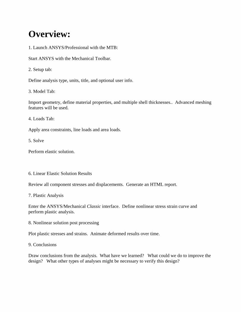
Overview: 1. Launch ANSYS/Professional with the MTB:

Start ANSYS with the Mechanical Toolbar.

2. Setup tab:

Define analysis type, units, title, and optional user info.

3. Model Tab:

Import geometry, define material properties, and multiple shell thicknesses.. Advanced meshing features will be used.

4. Loads Tab:

Apply area constraints, line loads and area loads.

5. Solve

Perform elastic solution.

6. Linear Elastic Solution Results

Review all component stresses and displacements. Generate an HTML report.

7. Plastic Analysis

Enter the ANSYS/Mechanical Classic interface. Define nonlinear stress strain curve and perform plastic analysis.

8. Nonlinear solution post processing

Plot plastic stresses and strains. Animate deformed results over time.

9. Conclusions

Draw conclusions from the analysis. What have we learned? What could we do to improve the design? What other types of analyses might be necessary to verify this design?

Step-by-step Instructions: Before beginning this problem, create a separate folder on your computer for this job and copy the suspension Parasolid part file suspension.xmt_txt to this folder.

If you do not have a parasolid translator, copy the file suspension.db instead. When you reach section 3.1 (Model Import), select ANSYS (*db*) for type of file and import the suspension.db file.

1. Launch ANSYS/Professional

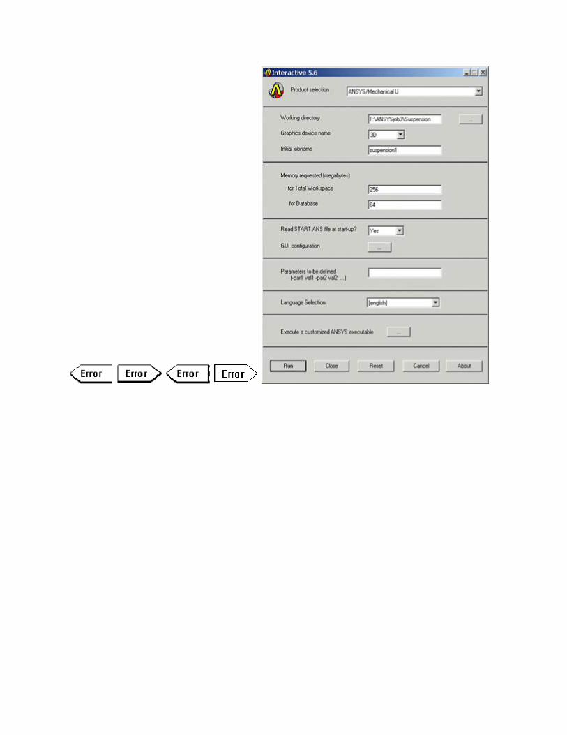
1.1. Launch ANSYS using your start menu.

A. Browse to select the working directory you just created for this job.

B. Enter a job name (suspension1). All ANSYS files created for this problem will have a filename of suspension1 followed by a unique extension.

C. Change the workspace and database sizes for this job to be 256 and 64 respectively.

D. Click RUN to start the ANSYS GUI.

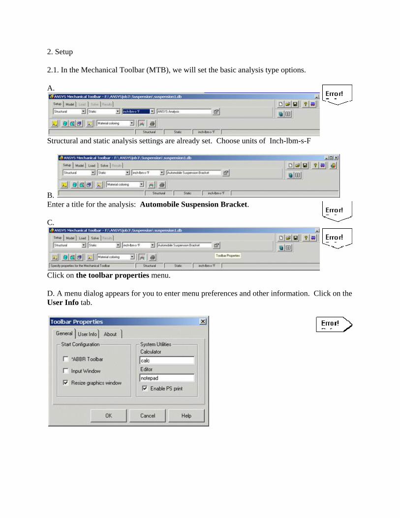
2. Setup

2.1. In the Mechanical Toolbar (MTB), we will set the basic analysis type options.

A.

Structural and static analysis settings are already set. Choose units of Inch-lbm-s-F

B. Enter a title for the analysis: Automobile Suspension Bracket.

C.

Click on the toolbar properties menu.

D. A menu dialog appears for you to enter menu preferences and other information. Click on the User Info tab.

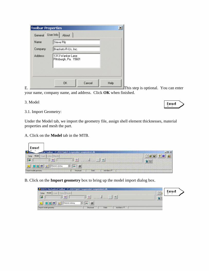
E. This step is optional. You can enter your name, company name, and address. Click OK when finished.

3. Model

3.1. Import Geometry:

Under the Model tab, we import the geometry file, assign shell element thicknesses, material properties and mesh the part.

A. Click on the Model tab in the MTB.

B. Click on the Import geometry box to bring up the model import dialog box.

C. Change the Files of type: option to Parasolid.

D. In the file list, highlight the file named suspension.xmt_txt. If you do not have a parasolid translator, select ANSYS (*db*) for type of file and import the suspension.db file.

E. Click Open.

F. Another dialog box will open asking you to choose import options. Select Shell or 2-D Solid.

G. Leave the No model clean-up (faster) option set.

H. Click OK.

I. ANSYS will import the Parasolid file and draw the part in the graphics window. Use the dynamic viewing controls to view all portions of the model.

3.2. Model Thickness

A. A pop up dialog box will come up for you to input a default property name and thickness for the model. Let's call this property Frame and use a thickness of 0.0875.

B. Click OK.

C. We need to assign this property to the model. Click on the Assign Shape dialog box.

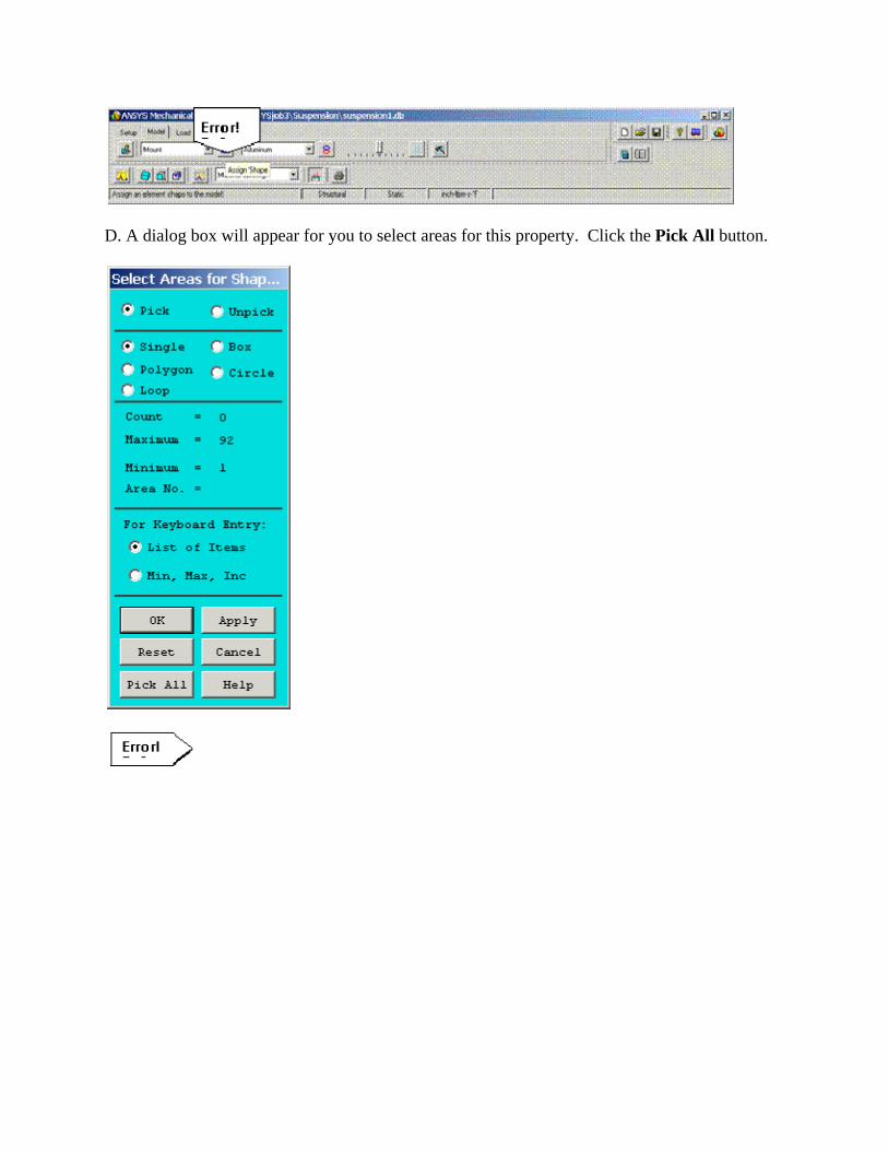
D. A dialog box will appear for you to select areas for this property. Click the Pick All button.

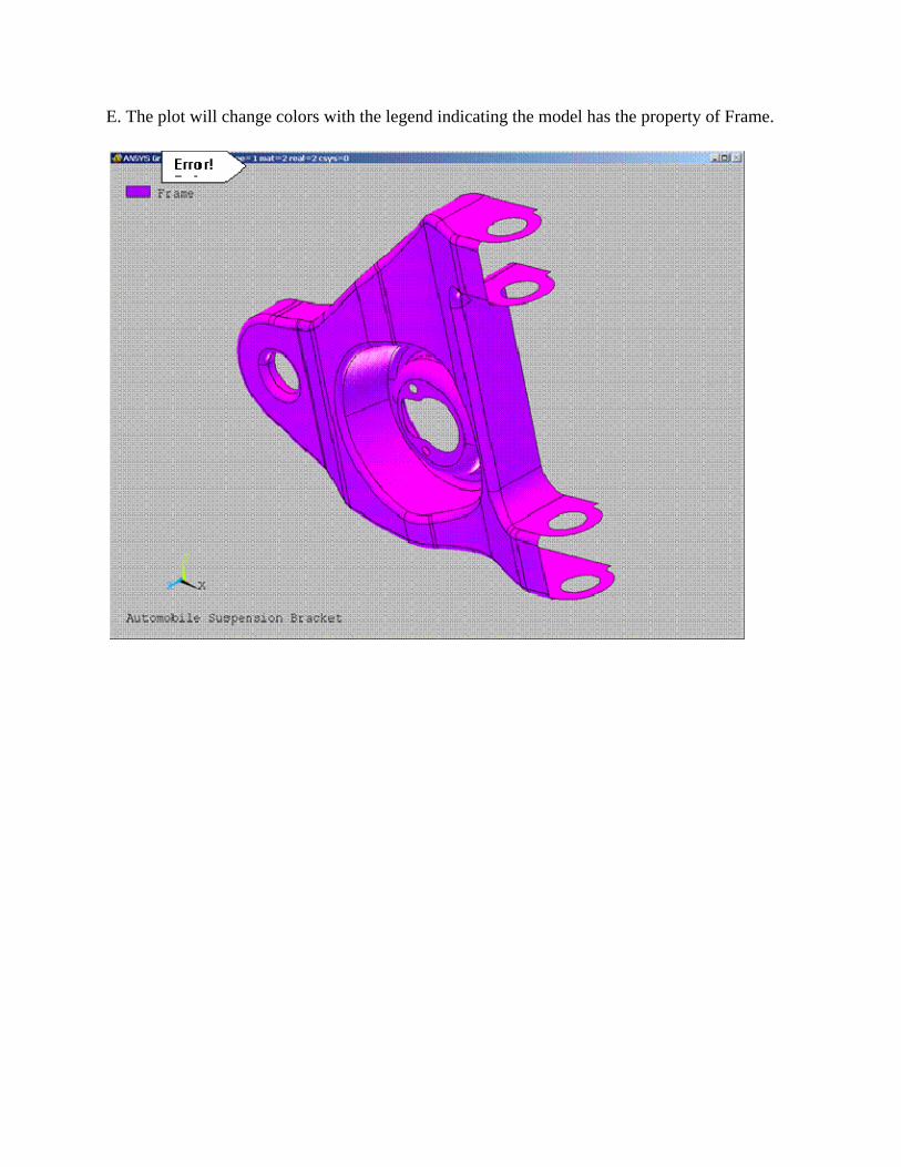
E. The plot will change colors with the legend indicating the model has the property of Frame.

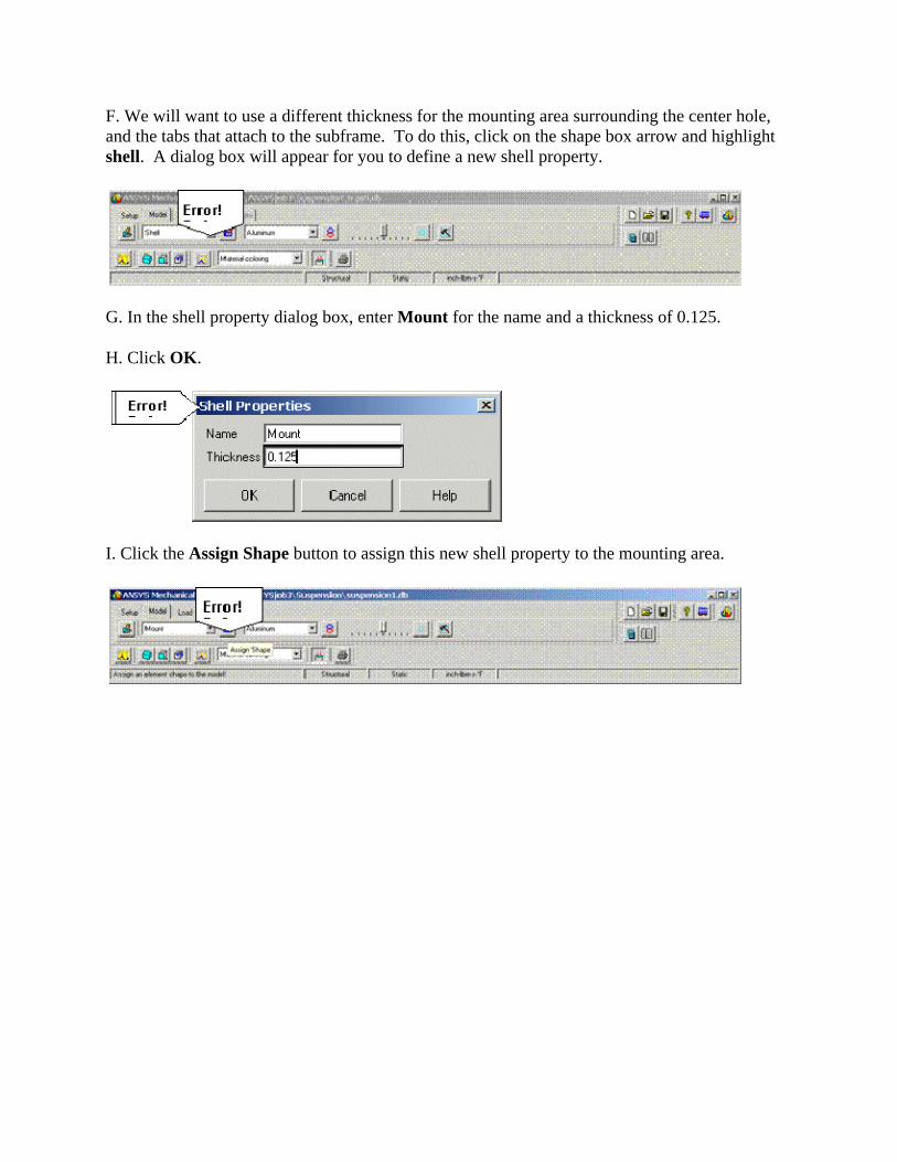
F. We will want to use a different thickness for the mounting area surrounding the center hole, and the tabs that attach to the subframe. To do this, click on the shape box arrow and highlight shell. A dialog box will appear for you to define a new shell property.

G. In the shell property dialog box, enter Mount for the name and a thickness of 0.125.

H. Click OK.

I. Click the Assign Shape button to assign this new shell property to the mounting area.

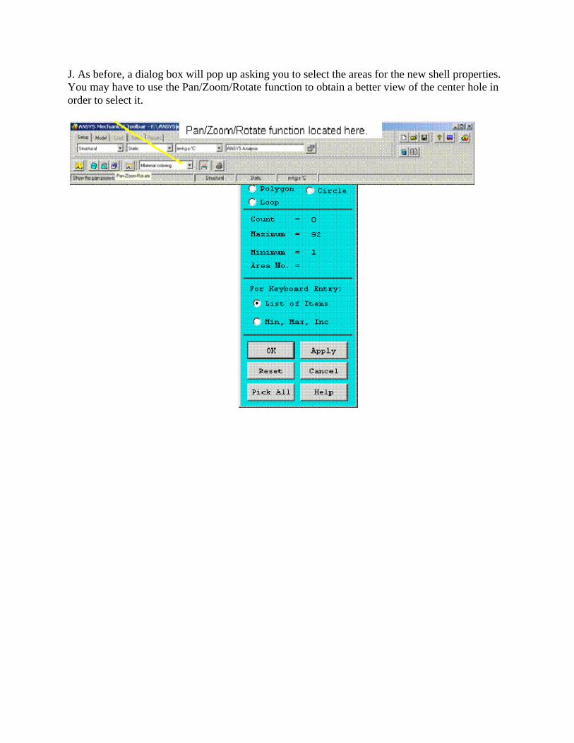
J. As before, a dialog box will pop up asking you to select the areas for the new shell properties. You may have to use the Pan/Zoom/Rotate function to obtain a better view of the center hole in order to select it.

K. Use the mouse to select the areas shown below. There are three areas at the center hole. Click near the center to select the keyhole shaped area, and off to the sides to select the two fillet areas surrounding the center hole. Hold down the left button and drag the mouse until the proper area is highlighted. The selection will be made when you release the button.

L. Also select the four holes, which make up the tabs that mount to the subframe.

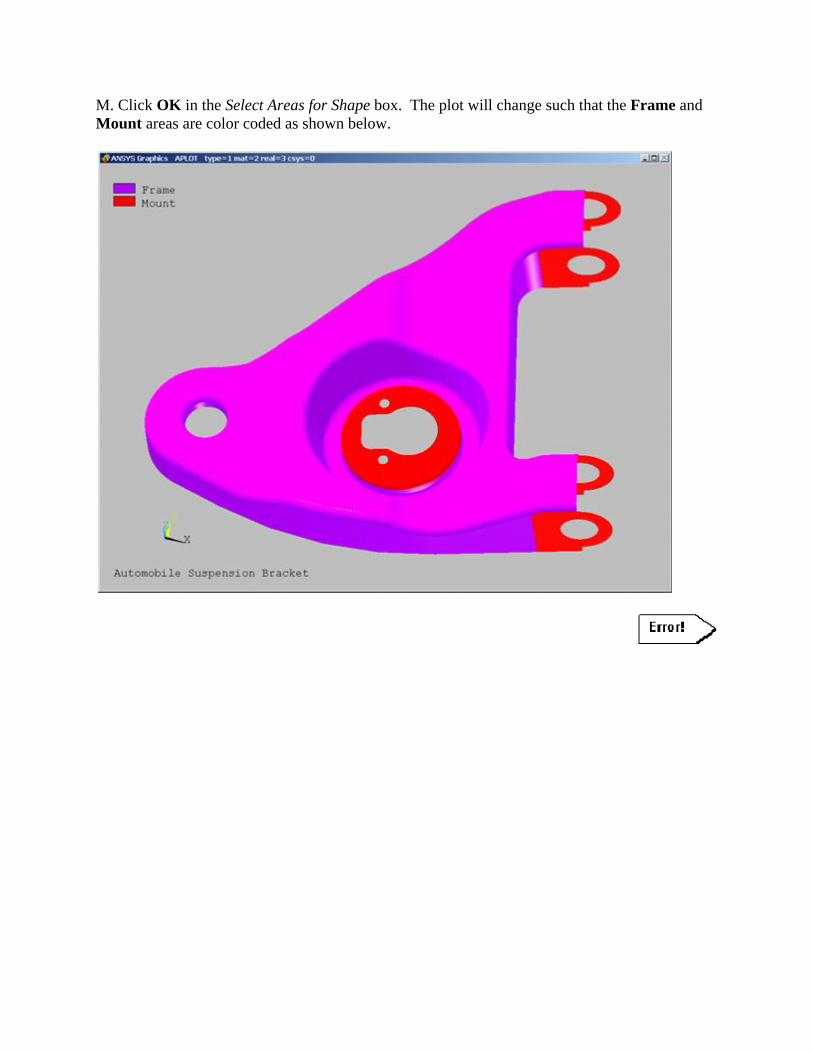
M. Click OK in the Select Areas for Shape box. The plot will change such that the Frame and Mount areas are color coded as shown below.

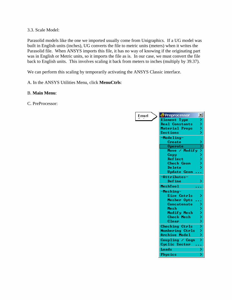
3.3. Scale Model:

Parasolid models like the one we imported usually come from Unigraphics. If a UG model was built in English units (inches), UG converts the file to metric units (meters) when it writes the Parasolid file. When ANSYS imports this file, it has no way of knowing if the originating part was in English or Metric units, so it imports the file as is. In our case, we must convert the file back to English units. This involves scaling it back from meters to inches (multiply by 39.37).

We can perform this scaling by temporarily activating the ANSYS Classic interface.

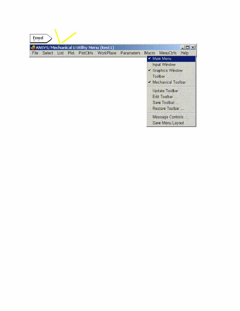
A. In the ANSYS Utilities Menu, click MenuCtrls:

B. Main Menu:

C. PreProcessor:

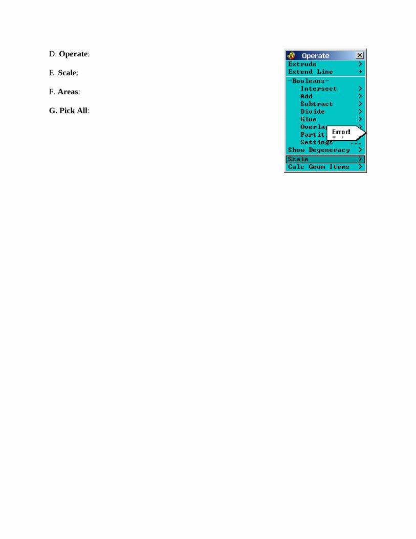
D. Operate:

E. Scale:

F. Areas:

G. Pick All:

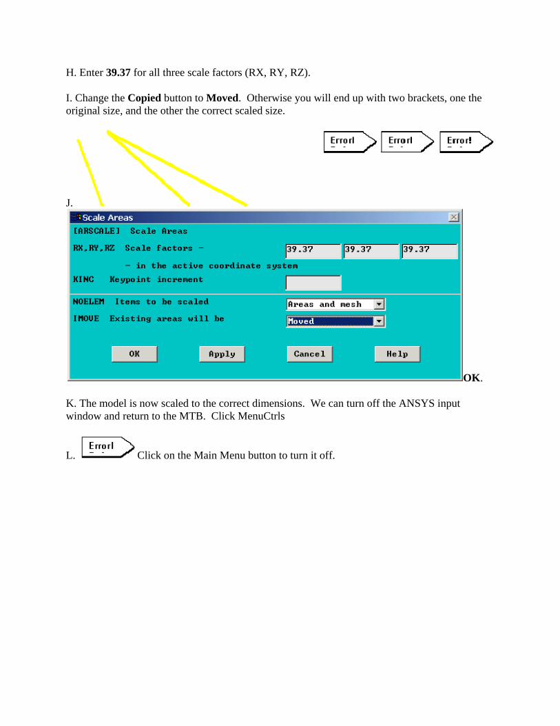
H. Enter 39.37 for all three scale factors (RX, RY, RZ).

I. Change the Copied button to Moved. Otherwise you will end up with two brackets, one the original size, and the other the correct scaled size.

J.

OK.

K. The model is now scaled to the correct dimensions. We can turn off the ANSYS input window and return to the MTB. Click MenuCtrls

L. Click on the Main Menu button to turn it off.

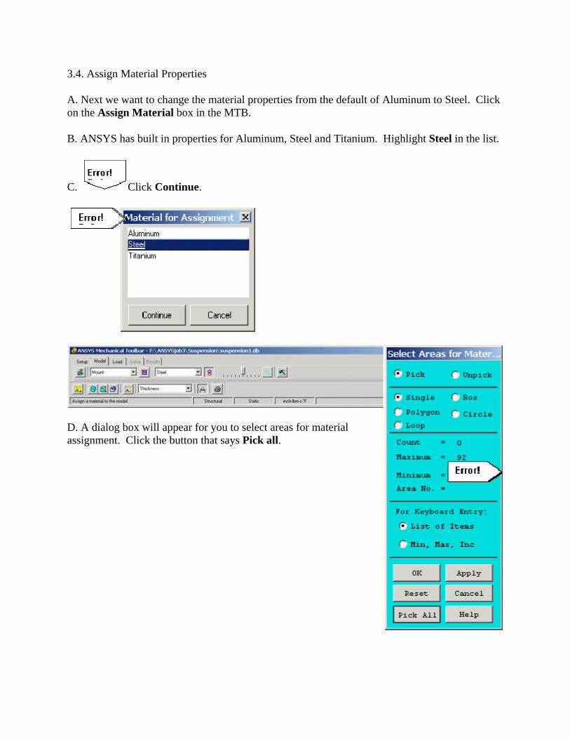
3.4. Assign Material Properties

A. Next we want to change the material properties from the default of Aluminum to Steel. Click on the Assign Material box in the MTB.

B. ANSYS has built in properties for Aluminum, Steel and Titanium. Highlight Steel in the list.

C. Click Continue.

D. A dialog box will appear for you to select areas for material assignment. Click the button that says Pick all.

E. The plot will change color with the legend indicating that the entire part is Steel.

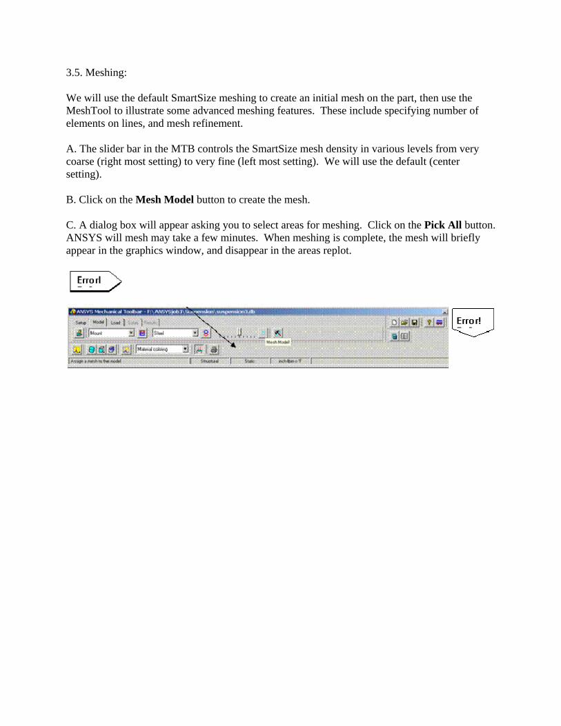
3.5. Meshing:

We will use the default SmartSize meshing to create an initial mesh on the part, then use the MeshTool to illustrate some advanced meshing features. These include specifying number of elements on lines, and mesh refinement.

A. The slider bar in the MTB controls the SmartSize mesh density in various levels from very coarse (right most setting) to very fine (left most setting). We will use the default (center setting).

B. Click on the Mesh Model button to create the mesh.

C. A dialog box will appear asking you to select areas for meshing. Click on the Pick All button. ANSYS will mesh may take a few minutes. When meshing is complete, the mesh will briefly appear in the graphics window, and disappear in the areas replot.

.

D. In the MTB, click and hold on the Area Plot button momentarily until the fly-out options appear.

E.

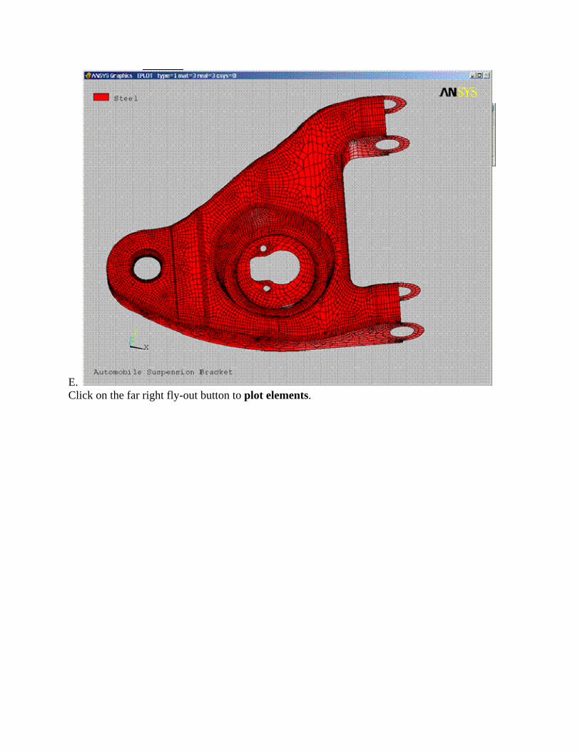
E. Click on the far right fly-out button to plot elements.

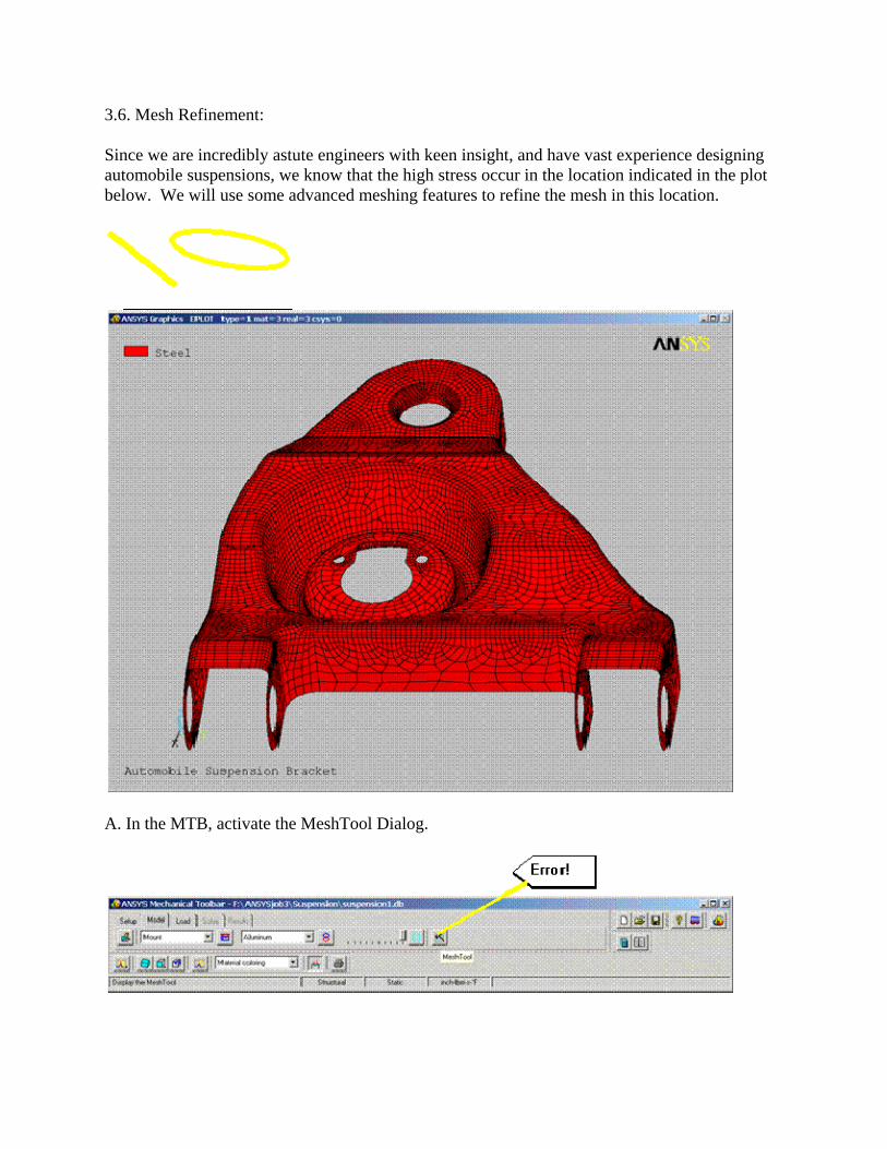
3.6. Mesh Refinement:

Since we are incredibly astute engineers with keen insight, and have vast experience designing automobile suspensions, we know that the high stress occur in the location indicated in the plot below. We will use some advanced meshing features to refine the mesh in this location.

A. In the MTB, activate the MeshTool Dialog.

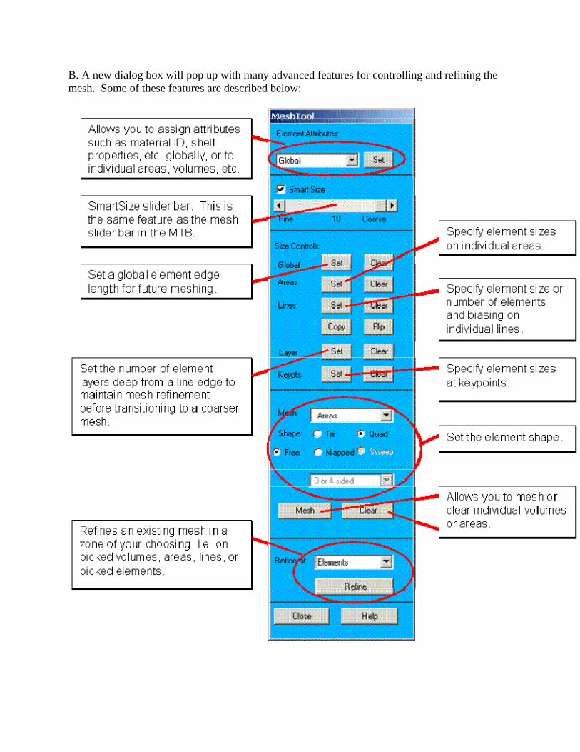
B. A new dialog box will pop up with many advanced features for controlling and refining the mesh. Some of these features are described below:

C. Let's start by refining the mesh in the high stress zone indicated above. Near the bottom of MeshTool, change the Refine at: Elements to Areas.

D. Click the Refine button.

E. A dialog box will appear asking you to select areas for refinement.

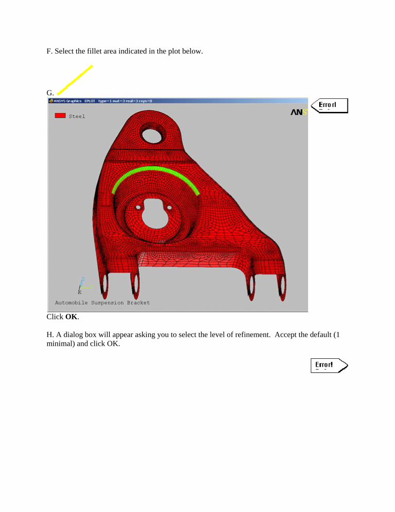
F. Select the fillet area indicated in the plot below.

G.

Click OK.

H. A dialog box will appear asking you to select the level of refinement. Accept the default (1 minimal) and click OK.

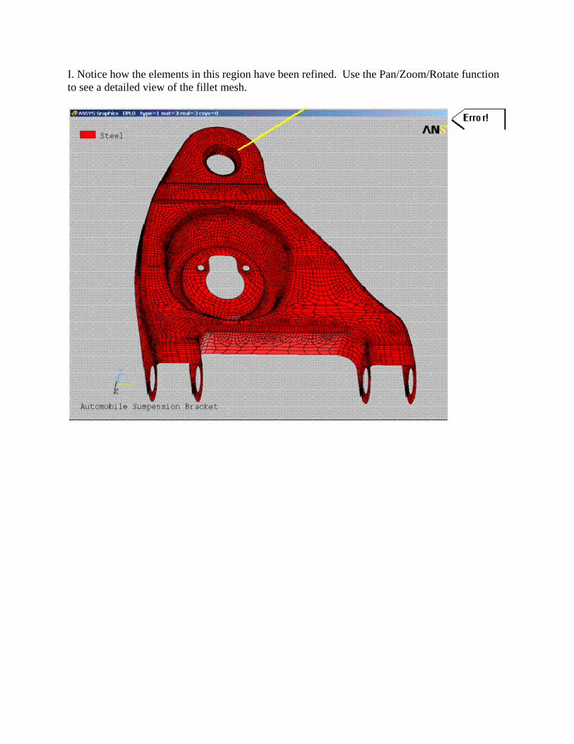
I. Notice how the elements in this region have been refined. Use the Pan/Zoom/Rotate function to see a detailed view of the fillet mesh.

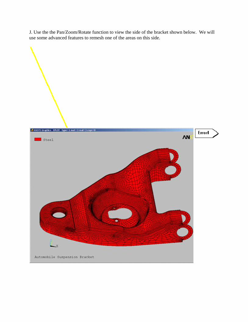
J. Use the the Pan/Zoom/Rotate function to view the side of the bracket shown below. We will use some advanced features to remesh one of the areas on this side.

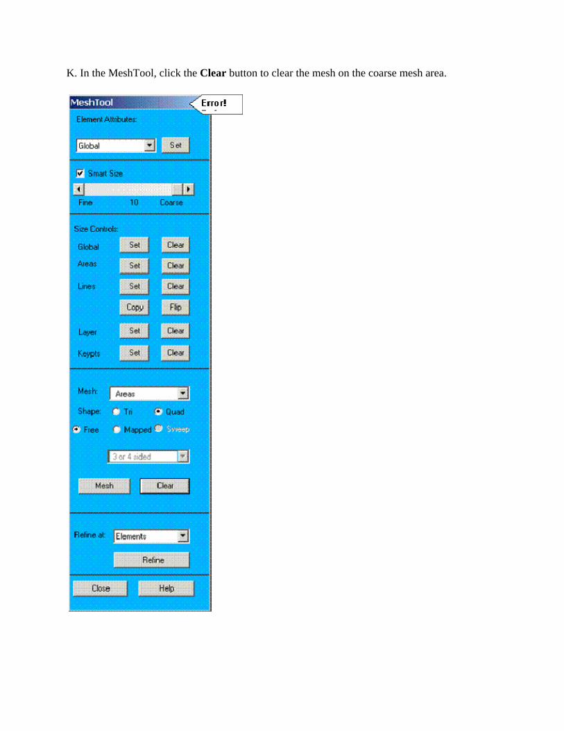
K. In the MeshTool, click the Clear button to clear the mesh on the coarse mesh area.

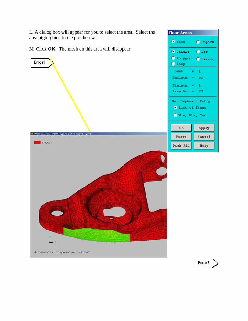
L. A dialog box will appear for you to select the area. Select the area highlighted in the plot below.

M. Click OK. The mesh on this area will disappear.

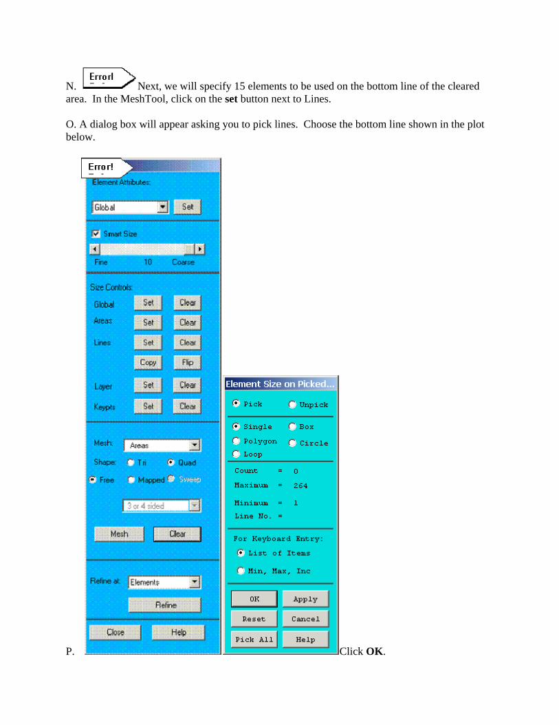
N. Next, we will specify 15 elements to be used on the bottom line of the cleared area. In the MeshTool, click on the set button next to Lines.

O. A dialog box will appear asking you to pick lines. Choose the bottom line shown in the plot below.

P. Click OK.

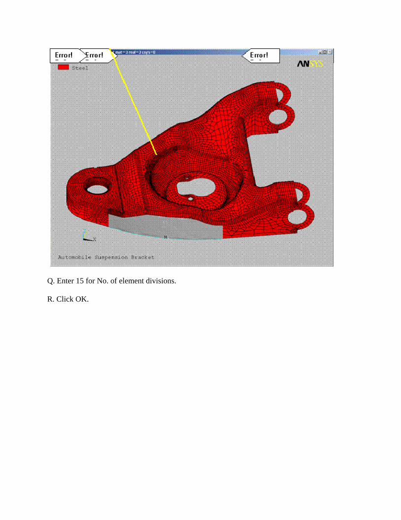
Q. Enter 15 for No. of element divisions.

R. Click OK.

S. Now we will remesh the area. Click on the mesh button. A dialog box will appear asking you to select the area for meshing.

T. Click on the area to be meshed shown in the plot below.

U. Click OK. The new mesh should look like the one in the plot below.

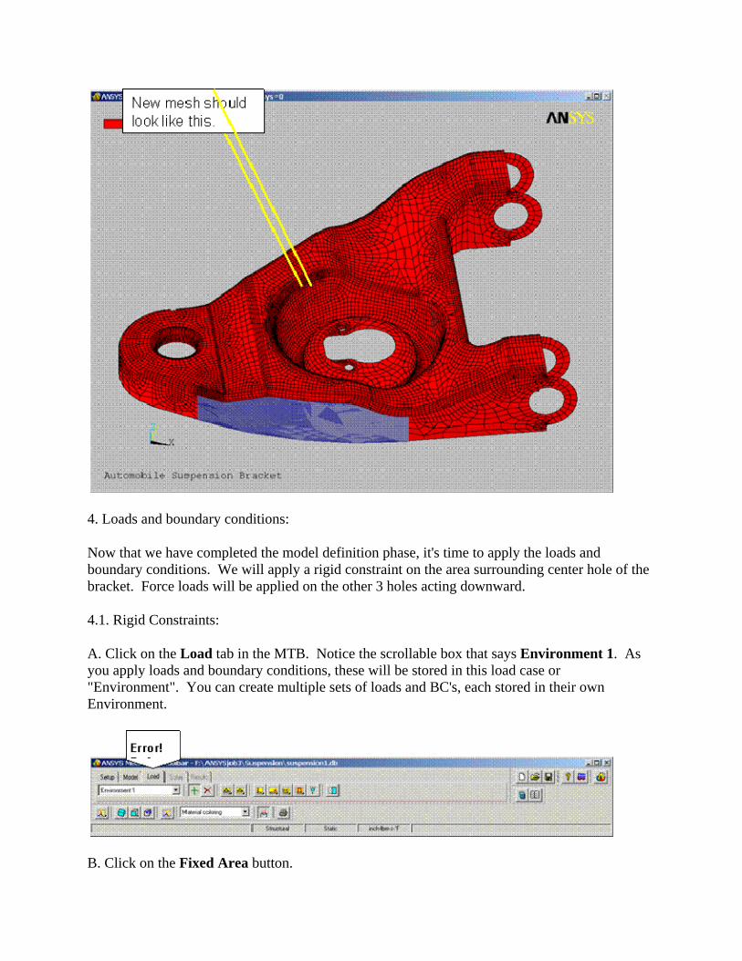
4. Loads and boundary conditions:

Now that we have completed the model definition phase, it's time to apply the loads and boundary conditions. We will apply a rigid constraint on the area surrounding center hole of the bracket. Force loads will be applied on the other 3 holes acting downward.

4.1. Rigid Constraints:

A. Click on the Load tab in the MTB. Notice the scrollable box that says Environment 1. As you apply loads and boundary conditions, these will be stored in this load case or "Environment". You can create multiple sets of loads and BC's, each stored in their own Environment.

B. Click on the Fixed Area button.

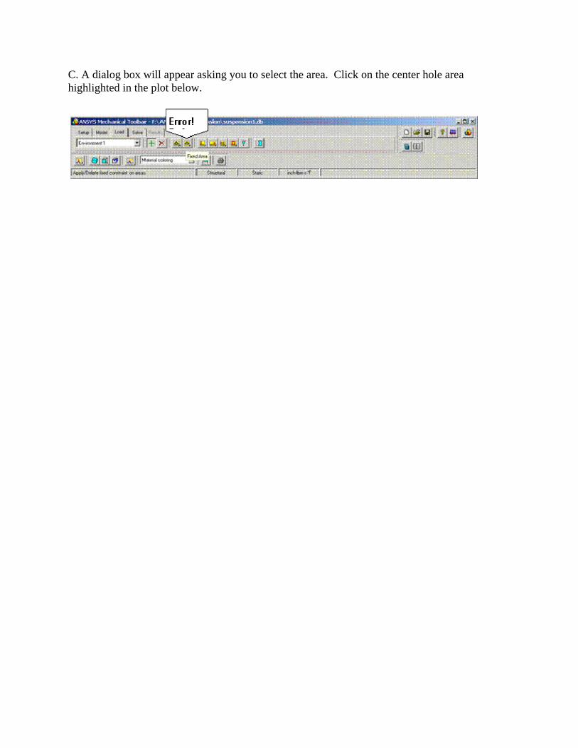
C. A dialog box will appear asking you to select the area. Click on the center hole area highlighted in the plot below.

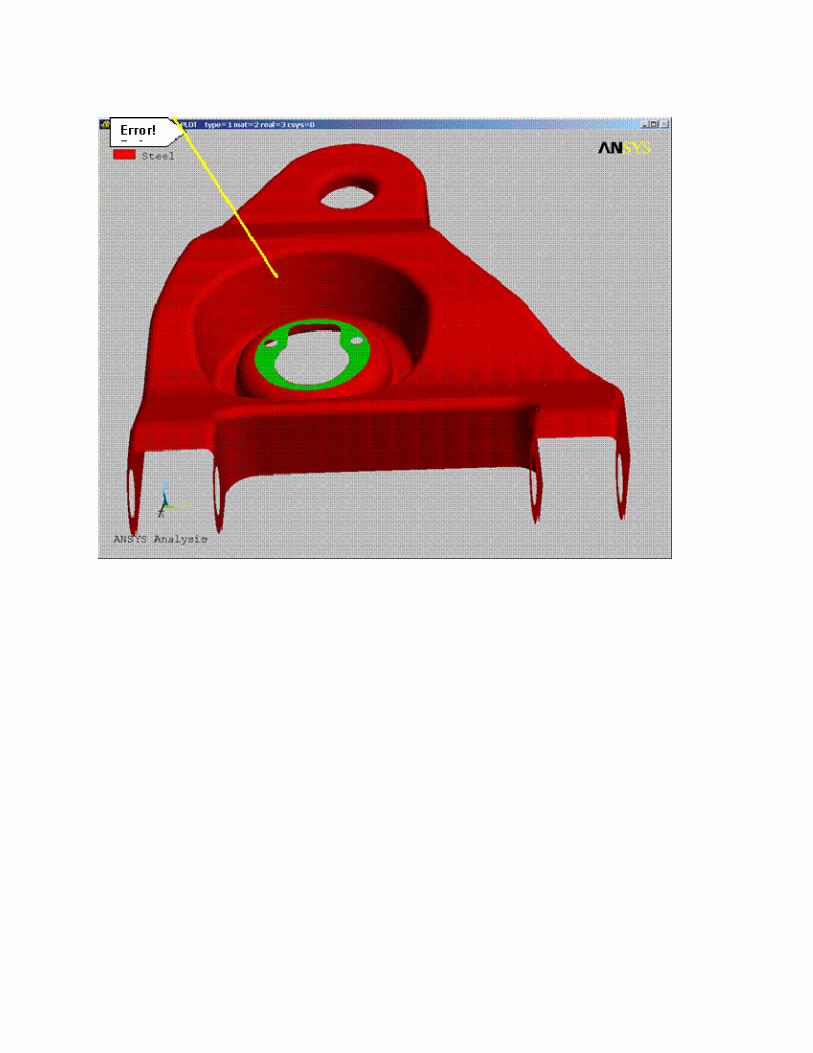
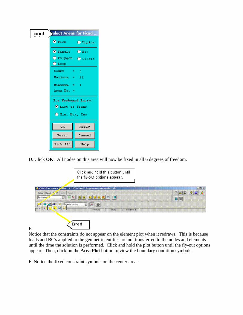
D. Click OK. All nodes on this area will now be fixed in all 6 degrees of freedom.

E. Notice that the constraints do not appear on the element plot when it redraws. This is because loads and BC's applied to the geometric entities are not transferred to the nodes and elements until the time the solution is performed. Click and hold the plot button until the fly-out options appear. Then, click on the Area Plot button to view the boundary condition symbols.

F. Notice the fixed constraint symbols on the center area.

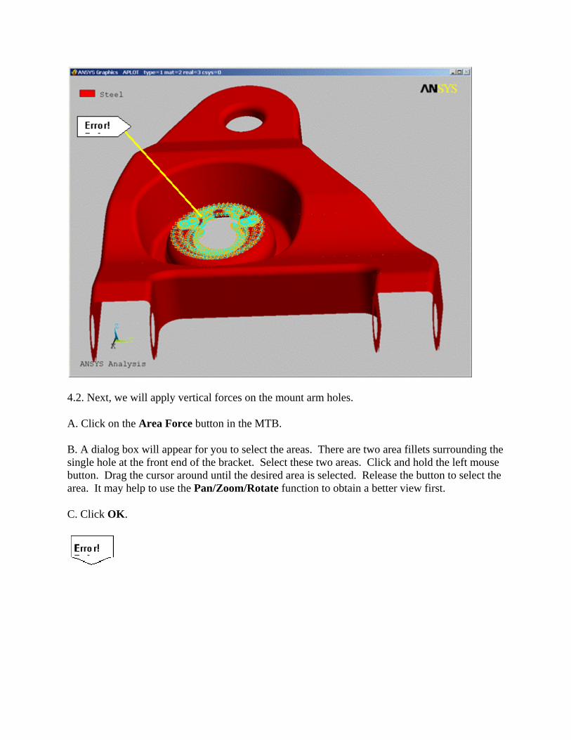
4.2. Next, we will apply vertical forces on the mount arm holes.

A. Click on the Area Force button in the MTB.

B. A dialog box will appear for you to select the areas. There are two area fillets surrounding the single hole at the front end of the bracket. Select these two areas. Click and hold the left mouse button. Drag the cursor around until the desired area is selected. Release the button to select the area. It may help to use the Pan/Zoom/Rotate function to obtain a better view first.

C. Click OK.

D. Another dialog box will appear for you to enter the force direction and values. The vertical direction is Z. We want to apply a total force of 600 pounds acting downward. Enter a value of -600 in the Z direction box.

E. Click OK. The force will be distributed such that a uniform total load of 600 pounds acts on two areas.

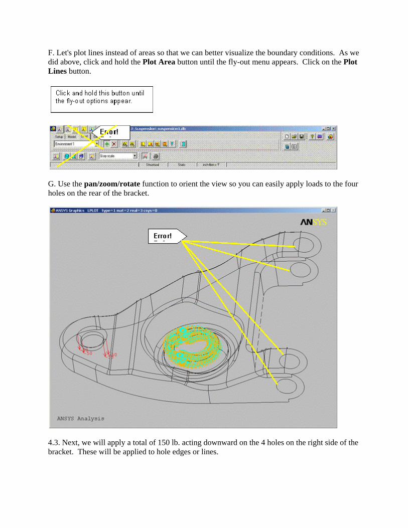
F. Let's plot lines instead of areas so that we can better visualize the boundary conditions. As we did above, click and hold the Plot Area button until the fly-out menu appears. Click on the Plot Lines button.

G. Use the pan/zoom/rotate function to orient the view so you can easily apply loads to the four holes on the rear of the bracket.

4.3. Next, we will apply a total of 150 lb. acting downward on the 4 holes on the right side of the bracket. These will be applied to hole edges or lines.

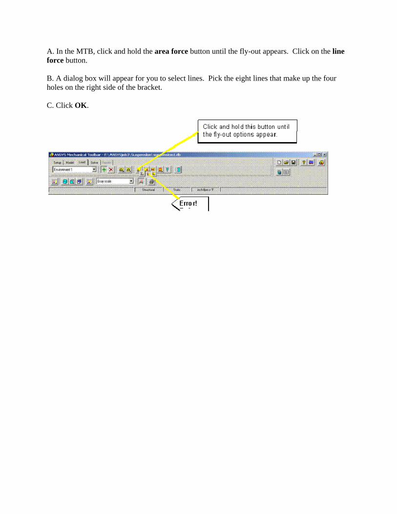
A. In the MTB, click and hold the area force button until the fly-out appears. Click on the line force button.

B. A dialog box will appear for you to select lines. Pick the eight lines that make up the four holes on the right side of the bracket.

C. Click OK.

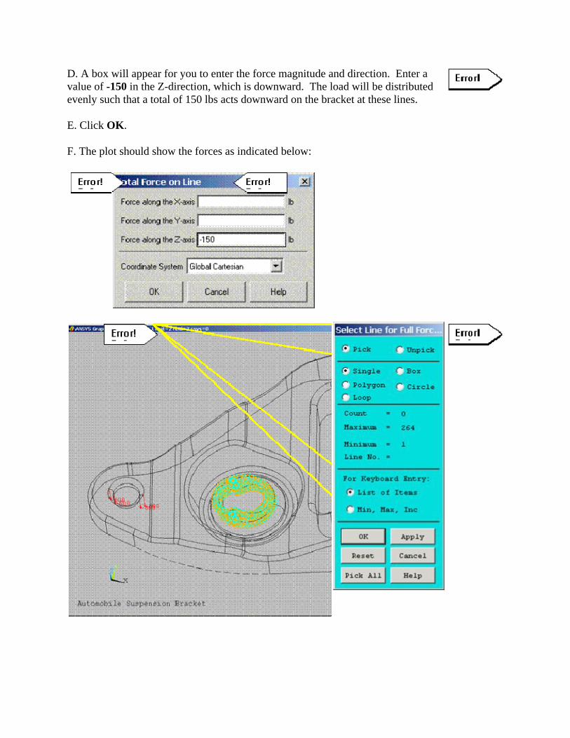
D. A box will appear for you to enter the force magnitude and direction. Enter a value of -150 in the Z-direction, which is downward. The load will be distributed evenly such that a total of 150 lbs acts downward on the bracket at these lines.

E. Click OK.

F. The plot should show the forces as indicated below:

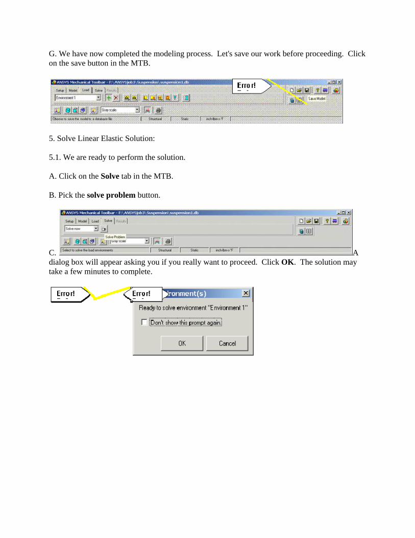
G. We have now completed the modeling process. Let's save our work before proceeding. Click on the save button in the MTB.

5. Solve Linear Elastic Solution:

5.1. We are ready to perform the solution.

A. Click on the Solve tab in the MTB.

B. Pick the solve problem button.

C. A dialog box will appear asking you if you really want to proceed. Click OK. The solution may take a few minutes to complete.

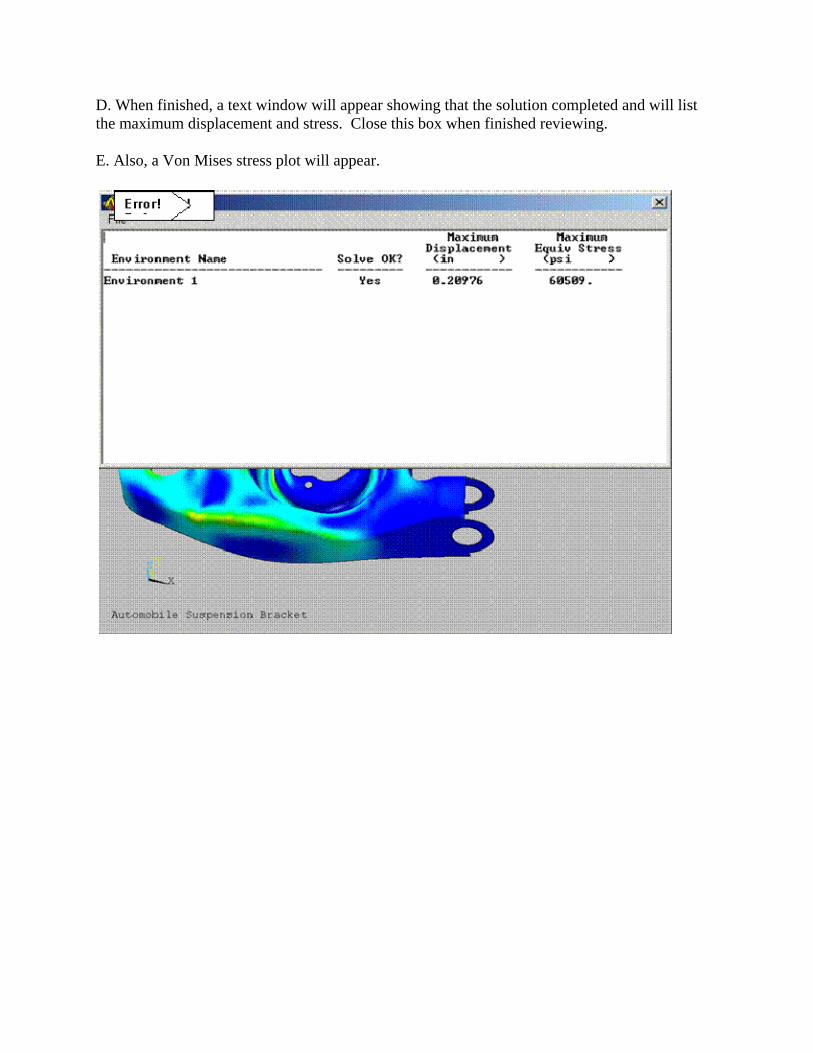
D. When finished, a text window will appear showing that the solution completed and will list the maximum displacement and stress. Close this box when finished reviewing.

E. Also, a Von Mises stress plot will appear.

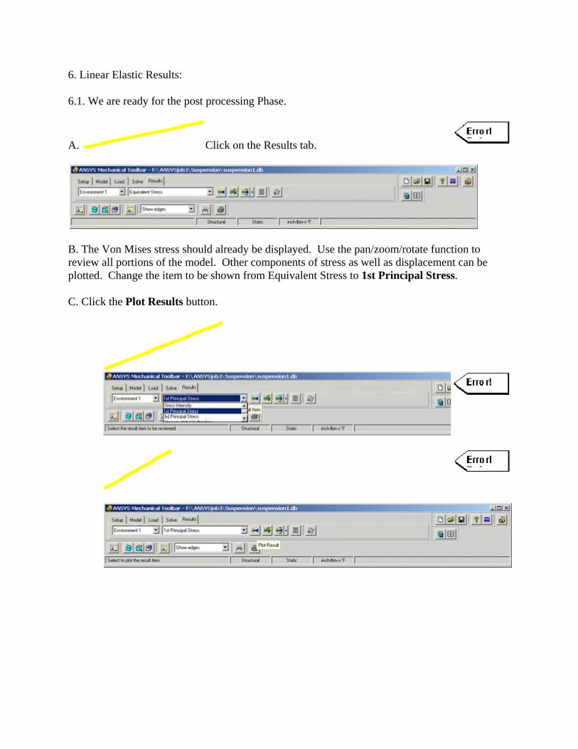
6. Linear Elastic Results:

6.1. We are ready for the post processing Phase.

A. Click on the Results tab.

B. The Von Mises stress should already be displayed. Use the pan/zoom/rotate function to review all portions of the model. Other components of stress as well as displacement can be plotted. Change the item to be shown from Equivalent Stress to 1st Principal Stress.

C. Click the Plot Results button.

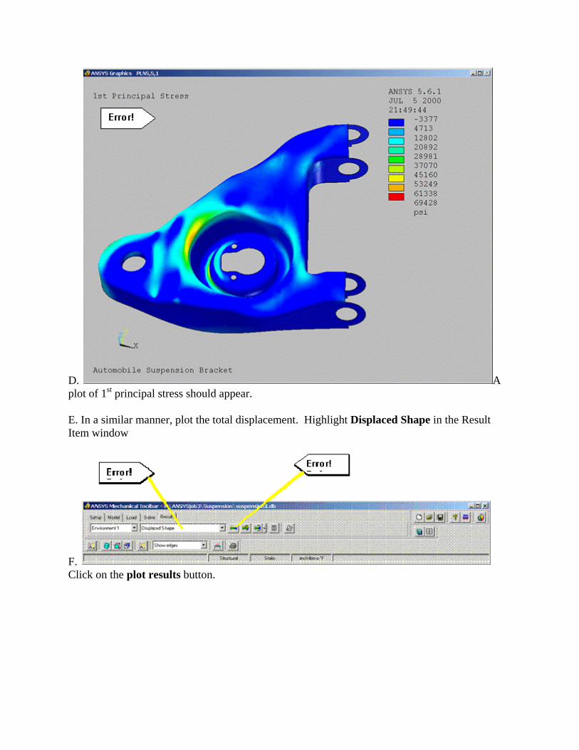
D. A plot of 1st principal stress should appear.

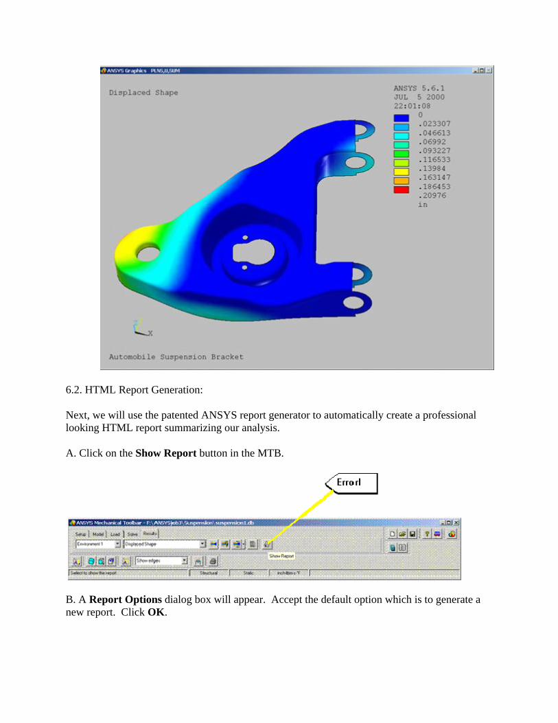
E. In a similar manner, plot the total displacement. Highlight Displaced Shape in the Result Item window

F. Click on the plot results button.

6.2. HTML Report Generation:

Next, we will use the patented ANSYS report generator to automatically create a professional looking HTML report summarizing our analysis.

A. Click on the Show Report button in the MTB.

B. A Report Options dialog box will appear. Accept the default option which is to generate a new report. Click OK.

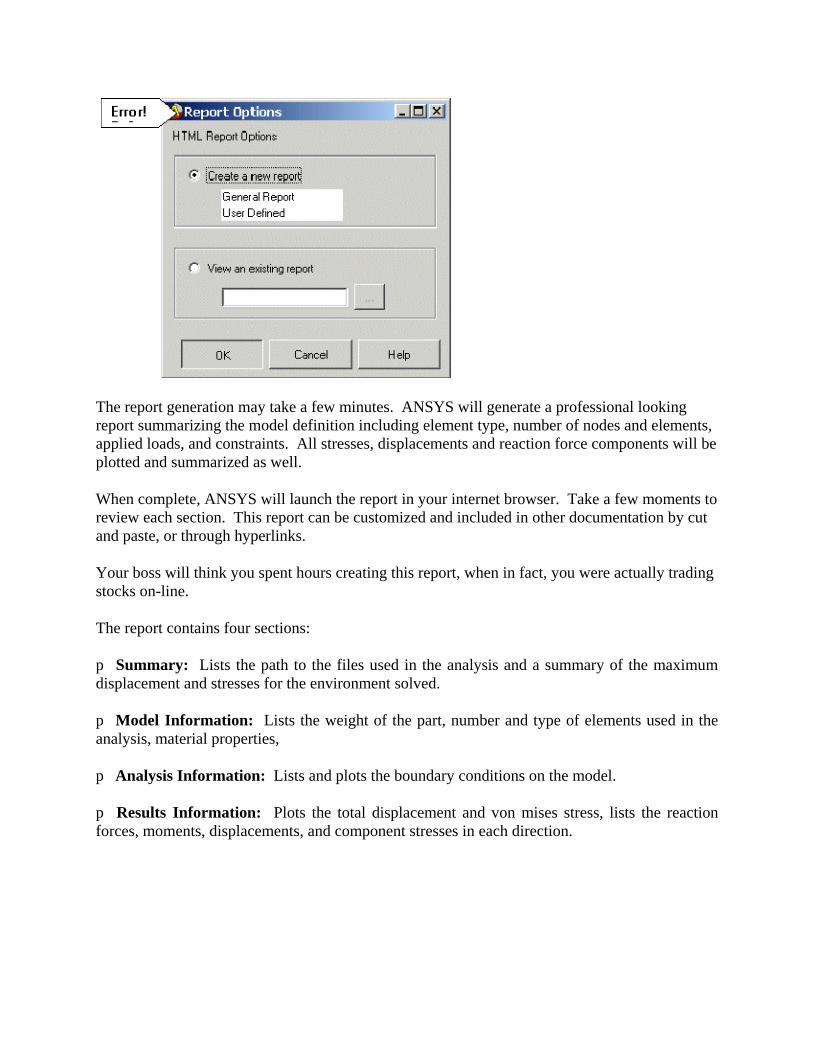
The report generation may take a few minutes. ANSYS will generate a professional looking report summarizing the model definition including element type, number of nodes and elements, applied loads, and constraints. All stresses, displacements and reaction force components will be plotted and summarized as well.

When complete, ANSYS will launch the report in your internet browser. Take a few moments to review each section. This report can be customized and included in other documentation by cut and paste, or through hyperlinks.

Your boss will think you spent hours creating this report, when in fact, you were actually trading stocks on-line.

The report contains four sections:

p Summary: Lists the path to the files used in the analysis and a summary of the maximum displacement and stresses for the environment solved.

p Model Information: Lists the weight of the part, number and type of elements used in the analysis, material properties,

p Analysis Information: Lists and plots the boundary conditions on the model.

p Results Information: Plots the total displacement and von mises stress, lists the reaction forces, moments, displacements, and component stresses in each direction.

7. Plastic Analysis:

7.1. ANSYS Classic Interface:

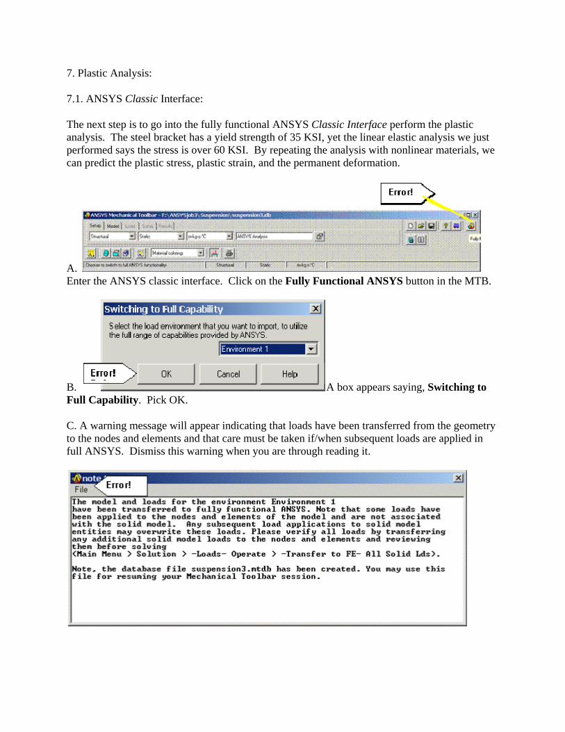
The next step is to go into the fully functional ANSYS Classic Interface perform the plastic analysis. The steel bracket has a yield strength of 35 KSI, yet the linear elastic analysis we just performed says the stress is over 60 KSI. By repeating the analysis with nonlinear materials, we can predict the plastic stress, plastic strain, and the permanent deformation.

A. Enter the ANSYS classic interface. Click on the Fully Functional ANSYS button in the MTB.

B. A box appears saying, Switching to Full Capability. Pick OK.

C. A warning message will appear indicating that loads have been transferred from the geometry to the nodes and elements and that care must be taken if/when subsequent loads are applied in full ANSYS. Dismiss this warning when you are through reading it.

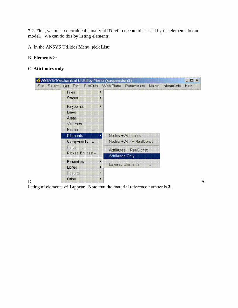
7.2. First, we must determine the material ID reference number used by the elements in our model. We can do this by listing elements.

A. In the ANSYS Utilities Menu, pick List:

B. Elements >:

C. Attributes only.

D. A listing of elements will appear. Note that the material reference number is 3.

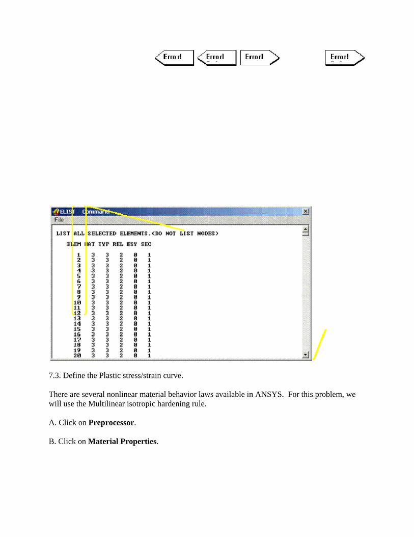
7.3. Define the Plastic stress/strain curve.

There are several nonlinear material behavior laws available in ANSYS. For this problem, we will use the Multilinear isotropic hardening rule.

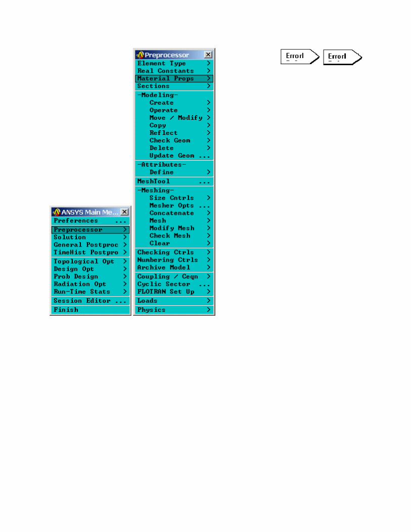
A. Click on Preprocessor.

B. Click on Material Properties.

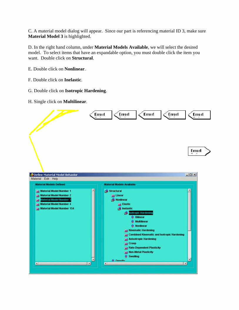
C. A material model dialog will appear. Since our part is referencing material ID 3, make sure Material Model 3 is highlighted.

D. In the right hand column, under Material Models Available, we will select the desired model. To select items that have an expandable option, you must double click the item you want. Double click on Structural.

E. Double click on Nonlinear.

F. Double click on Inelastic.

G. Double click on Isotropic Hardening.

H. Single click on Multilinear.

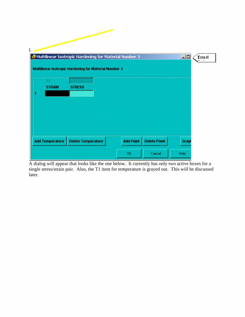
I.

A dialog will appear that looks like the one below. It currently has only two active boxes for a single stress/strain pair. Also, the T1 item for temperature is grayed out. This will be discussed later.

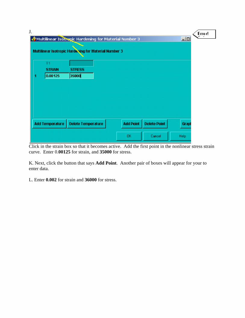
J.

Click in the strain box so that it becomes active. Add the first point in the nonlinear stress strain curve. Enter 0.00125 for strain, and 35000 for stress.

K. Next, click the button that says Add Point. Another pair of boxes will appear for your to enter data.

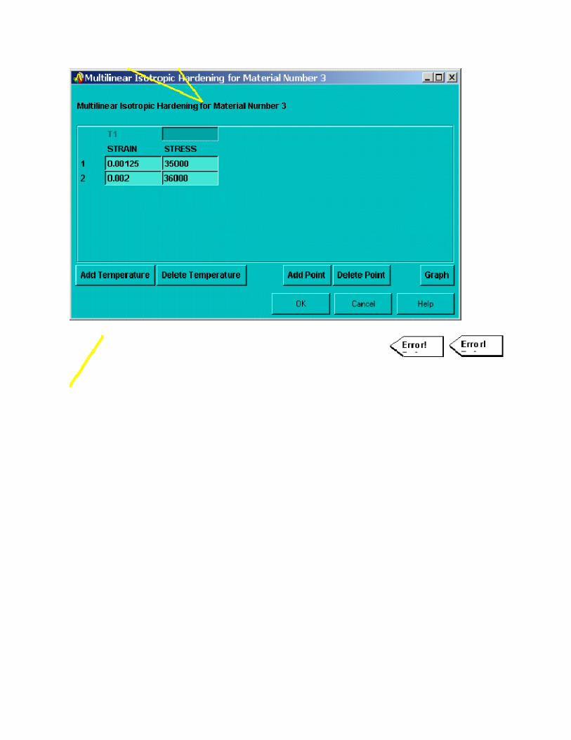
L. Enter 0.002 for strain and 36000 for stress.

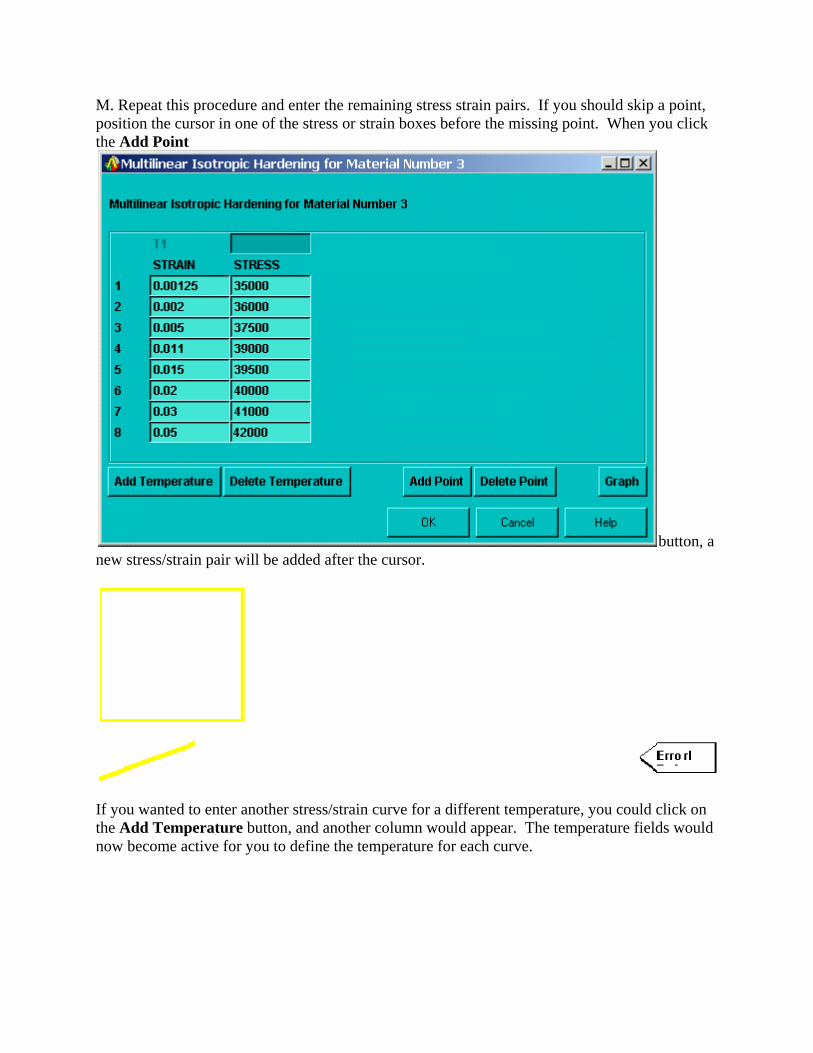
M. Repeat this procedure and enter the remaining stress strain pairs. If you should skip a point, position the cursor in one of the stress or strain boxes before the missing point. When you click the Add Point

button, a new stress/strain pair will be added after the cursor.

If you wanted to enter another stress/strain curve for a different temperature, you could click on the Add Temperature button, and another column would appear. The temperature fields would now become active for you to define the temperature for each curve.

N. Next, lets plot our stress strain curve to visually verify it. Pick the Graph button.

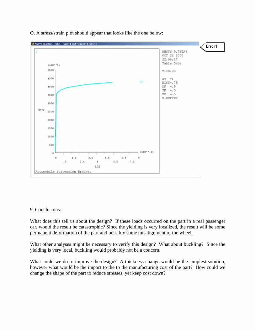
O. A stress/strain plot should appear that looks like the one below:

9. Conclusions:

What does this tell us about the design? If these loads occurred on the part in a real passenger car, would the result be catastrophic? Since the yielding is very localized, the result will be some permanent deformation of the part and possibly some misalignment of the wheel.

What other analyses might be necessary to verify this design? What about buckling? Since the yielding is very local, buckling would probably not be a concern.

What could we do to improve the design? A thickness change would be the simplest solution, however what would be the impact to the to the manufacturing cost of the part? How could we change the shape of the part to reduce stresses, yet keep cost down?