Automobile demand, model cycle and age effectspeople.bu.edu/jordij/papers/autdemand.pdfAutomobile demand, model cycle and age effects 1996, we observe the monthly registrations (sales)

Span Econ RevDOI 10.1007/s10108-006-9014-y

R E G U L A R A RT I C L E

Automobile demand, model cycle and age effects

María José Moral · Jordi Jaumandreu

© Springer-Verlag 2006

Abstract This paper is aimed at exploring the existence of typical patterns ofautomobile model life and the formal test for age effects in a discrete-choicedemand framework estimated with data on the models sold in the Spanish mar-ket. Estimates show that the evolution of market shares entails and quantifiesage effects resulting from consumer demand. These effects are clearly distin-guishable from the impacts generated by changes in attributes and firm pricing.They carry an exogenous factor that is full of implications for firm behaviourover the life of a model: the modification of demand price sensitivities. As aresult, for example, equilibrium own-price elasticities are observed to decreaseuntil the fourth year of a model life, and then to increase again.

JEL Classification D43

Keywords Model life cycle · Automobile demand · Discrete-choice ·Differentiated products

Introduction

Car model turnover is an important characteristic of the automobile market.The entry of new models and the exit of others over time are quantitatively

M. J. Moral (B)Universidad Nacional de Educación a Distancia,Dpto. de Economía Aplicada e Ha Económica,Senda del Rey 11, 28040 Madrid, Spaine-mail: [email protected]

J. JaumandreuDpto. de Economía, Madrid 126, 28903 Getafe, Spaine-mail: [email protected]

M. J. Moral and J. Jaumandreu

important. Moreover, the exit of a model and the entry of another are oftenthe two sides of a unique operation synchronized by their manufacturer. Hencethere exist life cycles of models. Some are short, others longer. The life ofextremely successful models is boosted by producers at certain moments in timewith changes in the current version, but old models are often simply replacedby new ones.

The life cycles of models must be seen as the result of the interaction betweenconsumers’ preferences and producers’ decisions, but consumers’ demand evo-lution is likely to play a crucial role. The presence of defined patterns of demandassociated with model age (the time that a model has been marketed) suggestsa likely explanation for market shares evolution over time. And consumers’age-related behaviour is likely to impact the price sensitivity of demand withrespect to the own-price of models and to the prices of competitor models. Aslong as firms react to these changes, the resulting equilibrium elasticities are,of course, endogenously determined, but the evolution of consumer demandcarries an important non-controlled factor of modification by the firm, giventhe remaining factors.

The purpose of this paper is to explore the effects of the age of a modelon automobile demand, both descriptively and using techniques of the dis-crete-choice approach to market demand estimation. In particular, we beginby looking at the characteristics of the life cycle of models by means of a non-parametric description of the relationships between model shares and modelages. Then we specify and test for the presence of age effects on the demandfor models using the discrete-choice framework [see Berry (1994) and Berry,Levinsohn and Pakes (1995) – hereafter BLP – for a paramount application tothe automobile market.1]

Consumer demand change with model age is likely to have important conse-quences for firm behaviour. Firstly, firms are likely to respond to these changesin the short run with (optimal) pricing adjustments. Secondly, firms are likely tocarry out minor model changes in order to try to enhance the durability of themodels. Thirdly, firms will adopt the exit–entry decisions of their models accord-ing to the impact of these changes on profits. The entry decisions of models areassociated with large sunk costs (design, plant adaptation, launch,. . .), and boththe decisions of new entry as well as the replacement of a model by another(cannibalisation) will be adopted only when the evolution of demand makesthis change profitable. All this makes the study of the age effects on demandan interesting step previous to undertaking more complete specifications of theforces underlying product decisions.

This study relies on a constructed panel data set for the Spanish car market,a particularly useful tool for studying model dynamics. Over the 7 years 1990–

1 The discrete-choice approach to demand estimation, developed for differentiated products mar-kets, has recently been enlarged, enriched, and applied extensively to the modelling of severalmarkets, in particular to the automobile market. Bresnahan’s (1987) automobile article can beconsidered a precedent of this type of model. Goldberg (1995), Feenstra and Levinsohn (1995),Verboven (1996), Berry et al. (1999, 2004), Goldberg and Verboven (2001) and Petrin (2002) includeautomobile demand estimations related to the discrete-choice method.


1996, we observe the monthly registrations (sales) of a total of 182 models,which account for virtually the entire market and are subject to a high turn-over. The data have been elaborated and matched to a database on prices andtechnical characteristics.

Results clearly show that car models have life cycles. Firstly, shares tend toincrease until the course of the fourth year in the life of a model. Secondly,shares subsequently tend to decrease as time goes by, and this deteriorationmay account for, on average, one third of its value. Thirdly, shares of surviv-ing models tend to be higher, denoting that firms decide to discontinue themodels with the worst evolution. On the other hand, we highlight the fact thatdemand age effects exist and are important in explaining shares patterns: oncemodel attributes, exogenous time demand determinants and price effects areaccounted for, age explains a significant part of the evolution of shares. In addi-tion, equilibrium elasticities betray the impact of model age: average elasticitiesdecrease during the three first years of model life and increase afterwards.

The rest of the paper is organized as follows. Age effects section discussesthe possible meaning of age effects in more detail and briefly relates this studyto other empirical findings. Car model turnover in the Spanish market sectionintroduces the data. Exploring model life cycle section is devoted to a descrip-tion of the models of life cycles by means of non-parametric analysis. Thedemand for models over time section explains the specification of age effects ina discrete choice framework, and Econometric estimation and results sectionpresents the estimation and results. Finally, Conclusion section concludes. Adata appendix gives some details on the sample and variables.

Age effects

Consumer demand evolution presumably has an important role in the life cyclesof models.2 In fact, there seem to be defined patterns of demand associated withmodel age, i.e., how long the car model stays on the market. Shares, as a matterof fact, tend to change over time much more pronouncedly than what can beexplained by observed relative model attributes.

One possible explanation is that consumers also valuate the degree to whichnew models possess disembodied attributes like “newness” or “latest design,”and old models possess “prestige” or “good reputation,” all of them attributesthat change with age. It may be that consumers simply like a series of minorembodied but unobservable technical features included in the newest modelsand judge them to be incorporated (or not) in enduring models. If this were thecase, the explanation for the evolution of market shares over time would be theevolution of average valuation with model age.

Most marketing literature on product life cycle, however, uses the alternative“adoption” approach. The path of sales over product age would be explained by

2 In general, demand change and technological progress interact in raising product life cycles [for ageneral presentation of cycles, mainly at the industry level, see Klepper (1996)]. However, productcycles present many industry-idiosyncratic characteristics.


the long-term purchasing behaviour of some consumers who act as “innovators”while others behave as “imitators.” See Kwoka (1996) for an application of thisapproach to the life cycle of minivans. But even if consumers do not differ intheir time readiness to buy newly introduced models, the choice sets of consum-ers may be changing as information about the new models spreads. See Goeree(2005) for an application of the impact of advertising on the enlargement of thechoice set of consumers in the computer market.

In practice, it seems difficult to disentangle these two explanations that prob-ably operate at the same time. And, in fact, it seems perfectly possible to testfor the presence of time effects and remain uncertain about the precise originof them. We are going to add the time effects to the usual linear utility spec-ification. In the first case, one can interpret the age effects as reflecting theevolution of the average valuation of consumers. In the second case, one cantake the age effects as a simple reduced form specification for the shift of therelevant distribution of consumers over time.

The effects of model age through changes of demand can be examined bystudying their impact on the elasticity of demand with respect to the own-priceof the model (and on the cross-price elasticities, i.e., the elasticities with respectto the prices of competing models.) As long as firms react optimally to thechanges in demand, price elasticities are, of course, variables endogenouslydetermined in equilibrium. They also depend on the firms’ decisions on prices,changing attributes and introducing models. But equilibrium elasticities are animportant tool for description and analysis (e.g., in the study of mark-ups), andhence the impact of age on (equilibrium) elasticities is worthy of assessmenteven in the absence of a structural model to separate all the effects.

In that sense, changes in price elasticities can help to understand differentphenomena that arise in these markets. For example, if a multiproduct firm facesown-price product sensitivities whose absolute value increases over time (andparallel exposure to rival price competition) it is likely to revise its product mixaccordingly. It may be in the firm’s interest to eventually substitute new prod-ucts for the oldest ones in order to preserve the maximisation of the expectedprofitability of the product mix that it sells. In the long run, the evolution ofelasticities and the effect of age are likely to be linked to all product decisions,from model improvements 3 to entry–exit decisions.

Only a few papers have directly addressed the life cycle of products intro-duced by multiproduct firms in a differentiated product industry, and mostof these papers have been devoted to industries experiencing a high prod-uct turnover derived from an intense process of innovations. Bresnahan et al.(1997) is perhaps the closest to our setting. Working within a discrete choicedemand framework, they study how two disembodied attributes of IBM-com-patible personal computers (being a “frontier” product, being branded) impactdemand elasticities and hence temporary market power, finding a role for thesetwo sources of differentiation. Davis (2006), which also uses a discrete-choice

3 Management literature stresses the importance of adopting techniques to enhance the durabilityof products.


demand model, introduces a time effect (weeks that a film is at a theater) as acharacteristic. Other studies have instead focused directly on the description ofthe entry and exit process, trying to assess determinants and choices. Amongthem, Stavins (1995) describes the positioning in the attributes’ space and theprobabilities of exit in personal computers, and Greenstein and Wade (1998)the product introduction determinants and hazard rates of mainframes. Animportant exception to the highly changing technological setting is Asplundand Sandin (1999), who study the Swedish beer market during the 1990s, amarket also characterised by a rapid product turnover. Studying hazard rates,they find patterns of product life and turnover that are very similar to the oneswe obtain in our demand framework.

Car model turnover in the Spanish market

This section briefly discusses the data and then characterises model turnoverduring the 1990s in the Spanish car market.

Car producers distinguish models, characterised by a model name, from theversions of these models, which they present as slight variations in the character-istics of the model. Our data set takes models, just as they have been defined byproducers, as the elemental units of analysis (see below for a detailed justifica-tion). The basic data consists of the breakdown of monthly new car registrations(sales) by models from January 1990 to December 1996 (an entry occurs whena new models appears.) A total of 182 models is covered (see Data appendix).

The information gathered for each model includes price (list retail price),attributes (for the attribute variables used in this paper, see Table 8) and thevariable that is crucial to our analysis: age. This variable measures in monthshow long, at time t, a model has been on the Spanish automobile market.

We group models into five categories that closely resemble common indus-try and marketing classifications. The classes considered are: small, compact,intermediate, luxury and minivan. For some purposes, we will also distinguishbetween the small “mini” or city cars, and the small “domestic” cars, the verypopular, somewhat superior models produced domestically. The number ofmodels in each segment is, respectively, 33, 37, 56, 47 and 9.4 We will distin-guish between “domestic” and “foreign” cars, by employing standard demand(not supply) criteria. We will call “domestic” the models sold by the brandswhich have domestic production, neglecting the fact that some of them arereally produced abroad and imported. There are seven big (export-oriented)multinational manufacturers that produce domestically, but whose domesticoutput is subject to complex transnational decisions about how to allocate theproduction of the models geographically.5 We will call “foreign” the cars sold

4 This classification is close to those used by Verboven (1996) for European cars (mini and small,medium, large, executive, luxury and sports), and Goldberg (1995) for the American car market(subcompact, compact, intermediate, standard, luxury and sports.) The main differences are theaggregation of luxury and sports cars in a single class, and the specification of a class for minivans.5 Citroen, Ford, Opel, Peugeot, Renault, Seat and Volkswagen.


by the firms without any domestic production. Grouping together the modelsmanufactured by the same producer gives a total of 31 firms or brands, sevenwith domestic production and 24 foreign producers.

Models seem to be a basic product category, both for demand and supplyreasons. On the one hand, models have a name and an image, and firms investheavily in advertising their models. This implies that consumers basically chooseamong models, and that firms incur some demand-rooted sunk costs in launch-ing models. On the other hand, models also have some basic attributes thatremain fairly stable over time. As Table 1 illustrates, for our 182-model sample,these attributes seem to be related mainly to size and power characteristics.This strongly suggests that model launching also implies technology-relatedsunk costs (design, manufacturing facilities adaptation, etc.). Demand and costside sunk costs provide a rationale for firms to stay with their living models. Infact, life spans are, as we will see below, heterogeneous, and they can be spottedby minor modifications in model characteristics. Producers try to boost the lifeof models at certain moments with small changes.6

The ideal data for the exercise we want to perform are data with strong entryand exit of models. The Spanish car market of that time meets this requirement,as shown in Tables 2 and 3. There is an important increase in the number ofmarketed models (36%) and a rather high rate of model turnover (20%). Theevolution of the market over our sample period shows two other important facts(see Table 2): some significant demand variability and a fall in tariffs, perfectlyforeseeable years earlier, followed by the corresponding increase in foreign carpenetration. There was an important demand downturn in 1993 and, to a lesserextent, in 1995 (and also a fall in prices), and in 1990, 1991 and 1992, the tariffsfor EEC imports and non-EEC countries were gradually reduced.7 As a result,the share of domestic models tends to fall as of 1992, while the share of foreignmodels increases (from 18 to almost 25%).

Let us concentrate on model increase and turnover. Table 2 reports an impor-tant increase in the number of models marketed (36%) and the correspondingfall in sales per model, given the detrended demand. The net entry of modelsis especially important in the first half of the period, but continues until theend. Table 3 details gross entry and exit and the age distribution evolution. Ascan be seen in the last two rows, a high, rather stable yearly rate of turnover

6 BLP define models in their 20-year US sample by requiring, in addition to the same name, thatthe width, length, horsepower or wheelbase do not change by more than 10%. Comparing our datawith BLP data, it turns out that we observe more or less the same cross-sectional average numberof models (110 vs. 118), but also that a model lasts on average 4.2 years, while they observe a modellasting only 2.2 years. Of course, our definition of model is not the same (we only rely on the name)but, from Table 1, it can be verified that the adoption of similar criteria to BLP would have a smalleffect (in fact it would only reduce our average number of years from 4.2 to 3.3). This seems to saythat our turnover level is not so high by US standards.7 The tariffs for the EEC imports were gradually reduced to 13.1, 8.7 and 4.4%, disappearing thefollowing year. The tariffs for the non-EEC countries were reduced during the same years to 23.1,18.8 and 14.4% and have been fixed at 10.3% since 1993.


Table 1 Degree of stability in model characteristics (no. and percentage of models with significantchanges)a,b

Characteristics Extent of the change

2% 5% 10%

StableNo. cyl 7 (3.85) 7 (3.85) 7 (3.85)Length 21 (11.54) 7 (3.85) 0 (0.00)Width 16 (8.79) 5 (2.74) 2 (1.10)

VaryingFiscalp 42 (23.08) 29 (15.93) 15 (8.24)CC 44 (24.17) 39 (21.43) 29 (15.93)Luggage 47 (25.82) 40 (21.97) 29 (15.93)

Greatly varyingHP 77 (42.31) 69 (37.91) 55 (30.22)RPM 64 (35.16) 49 (26.92) 18 (9.89)Maxspeed 74 (40.66) 38 (20.88) 11 (6.04)C90 83 (45.60) 64 (35.16) 39 (21.42)C120 81 (44.50) 59 (32.42) 39 (21.42)Ctown 79 (43.41) 62 (34.07) 38 (20.88)Weight 73 (40.11) 59 (32.42) 25 (13.73)

aEvery column reports the number (percentage) of models that fail to pass the correspondingstability test. The test is passed if the characteristic does not change by more than, respectively, 2,5 or 10% in a period of 12 months or lessbThe definitions of the variables are in Table 8 of the Data appendix

Table 2 The Spanish car market in the 1990s

Year Registrations Indexa No. of models Average monthly Priceb Sales ofsales by model domestic

modelsc

1990 971,466 109.7 98 851 1.976 82.01991 878,594 99.2 106 712 1.948 80.01992 973,414 109.9 117 700 1.876 81.31993 737,938 83.3 120 520 1.928 80.21994 901,754 101.8 124 616 1.925 78.71995 829,797 93.7 127 556 1.982 77.21996 906,444 102.3 133 580 1.986 75.2

aIndex = 100 at the time average of registrationsbSales-weighted mean price, in millions of pesetas circa 1992. The weight for each monthly modelobservation is the average share of the model in the corresponding yearcModels sold by firms with domestic production, regardless of whether they are imported

underlies net entry (entry + exit over the existing models is about 20%.8) As aresult, only one fourth of the models marketed by 1997 are models that werealready on the market at the beginning of the 1990s.

8 In total, many more models (103) enter than the number of models marketed before the begin-ning of the period (98 − 19 = 79.) But the exit of models is equally important (59), increasing afterthe two first years of the period, and tends to concentrate in some ages (from 4 to 8 years, say).


Table 3 Entry, age distribution of models and exit

Age (in years) 1990 1991 1992 1993 1994 1995 1996 Exitc: until1995 + 1996

Agea,b ≤ 1 19 10 16 12 13 17 161 < age ≤ 2 3 19 10 16 12 13 17 12 < age ≤ 3 7 3 19 10 16 11 13 43 < age ≤ 4 18 7 3 18 10 14 10 54 < age ≤ 5 5 18 6 3 18 7 13 6 + 25 < age ≤ 6 8 4 15 6 3 16 7 3 + 16 < age ≤ 7 6 8 4 13 6 3 15 5 + 37 < age ≤ 8 5 6 8 3 12 4 2 78 < age ≤ 9 6 4 6 6 2 10 3 89 < age ≤ 10 4 6 4 4 3 2 7 + 110 < age ≤ 11 4 4 6 4 4 3 2 411 < age ≤ 12 0 4 4 5 2 3 3 212 < age ≤ 13 1 0 3 3 5 2 3 213 < age ≤ 14 4 1 0 3 2 5 1 1 + 114 < age ≤ 15 3 4 1 0 3 2 4 + 115 < age ≤ 16 5 3 4 1 0 3 216 < age ≤ 17 5 3 4 1 0 317 < age ≤ 18 5 3 4 1 018 < age ≤ 19 5 3 4 1 119 < age ≤ 20 4 3 4 120 < age ≤ 21 3 321 < age ≤ 22 3

No. of models 98 106 117 119 124 127 133Totals

Entry 19d 10 16 12 13 17 16 103Exit 2 5 10 9 14 10 9 59

aThe first category represents a number of months equal to or less than 12bEach entry is the number of models of a given age observed during the yearcExits are equal to the difference between the number of models belonging to the interval of syears at time t and the number of models in the interval s + 1 years at time t + 1. Exits during 1996cannot be observed in this way and we report them separatelydIncludes the entry of eight models in January 1990. Four of them stay until the end of the sampleand the other four exit before December 1996

However, the market context implies that the study of model turnover mustbe carried out in a situation of increasing product competition interwovenwith a market opening (which probably triggered the new competitive inten-sity.) Accordingly, some remarks are pertinent. Firstly, it must be noted that theincrease in the number of products is mainly an endogenous outcome generatedby all the participants. For example, Asian producers account for a somewhatdisproportionate share of gross (and net) entry of models, but all firms contrib-ute to the increase in the number of models.9 Secondly, most of the productentry and exits come from the decisions to replace one model with another.

9 Asian producers market a number of new models (28) that almost doubles the initial numberaccounted for them (15), while the entry of models by domestic producers (28) and non-Asianforeign producers (48) approximately matches their initial contribution of models (35 and 48,respectively).


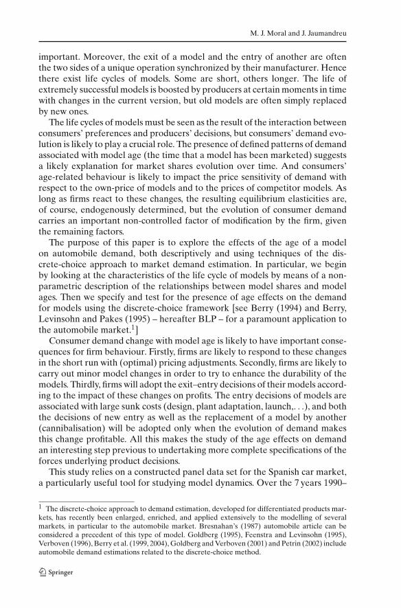
Table 4 Entry and exit of models by firms

Table 4, which reports all the entries and exits of the models, depicts the firms’entry–exit pairs that are only separated by one or, at most, 2 years’ delay. Thesepairs amount to more than 90% of the number of exits. Given these two char-acteristics, increased competition seems to have influenced the pace of modelintroduction more than changed its form. In principle, this justifies treating allthe models symmetrically.

Exploring model life cycle

The data set provides us with extensive information on the different phases ofthe life of models. We observe the entry of models, the market evolution ofmodels that have been marketed for different time intervals, and exit. In this


section, we focus on the simple description of the evolution of market sharesover model ages to detect and characterise average properties of the life cycleof models. To do this, we will employ non-parametric regression techniques.

Let s be the market share of a model at a given moment in time (we dropmodel and time subindices for simplicity), and let τ be its age or time elapsedfrom the moment that it was released on the market. Our first aim is to describemodel shares as a function of model age, that is, the expectation of model sharesconditional on τ , E( s | τ ).

For each model/month in the sample, we have a market share value thatis associated with the age of the model, which gives a total of 9,251 non-zeroshare-age observations. Moreover, for each model that exits the sample beforeDecember 1996, we complete its sample observations with the assignment ofa zero market share until reaching the maximum age that we will consider(180 + 84 = 264 months.) This is all we observe, because we have two types ofcensoring. For the non-exiting models, we cannot observe their shares from theirlast observation onwards (right censoring). We also cannot observe the early lifeobservations of the models, which were already on the market by January 1990(left censoring). To perform our descriptive exercises, we will pool together allthe non-censored (positive and zero) observations, which gives a total of 19,528observations. Interestingly enough, the density of these observations is ratheruniform throughout the ages considered (see Fig. 4)

The conditional expectation of s may be written by the law of iterated expec-tations as

E ( s | τ ) = P (s > 0 ) E ( s | τ , s > 0 ) + P (s = 0 ) E ( s | τ , s = 0 )

= P (s > 0 ) E ( s | τ , s > 0 )(1)

where the second equation follows from E(s|τ , s = 0) = 0. This expressionshows that the expected share is the result of two factors: the probability of stillbeing on the market for each age, or probability of survival, and the expectedshare conditional on age and survival. Therefore, to decompose and interpretthe expectation of s conditional on age, we will also estimate and study thesurvival function P ( s > 0 | τ ) and the expectation of s conditional on age andsurvival E ( s | τ , s > 0).

We non-parametrically estimate E(s|τ) and E(s|τ , s > 0) by means of thesimple Nadaraya-Watson estimator (see, for example, Wand and Jones 1995),using the entire sample and the subsample of positive shares, respectively. Toestimate the survival function, we compute the ratios at each τ of the numberof models with positive shares to the total number of observations for this age(see Kiefer 1988).

Figure 1 shows the result of estimating the expectation of s conditional onage. Figure 2 depicts the results of estimating the two components according toexpression (1) of this expectation. Panel a of Fig. 2 shows the estimation of thesurvival function and Panel b reports the result of estimating the expectationof s conditional on age and survival. Finally, the different panels of Fig. 3 givethe results of estimating the expectation of shares conditional on age in four car


Fig. 1 Conditional expectation function of shares. Shares are computed by taking the currentnumber of households at the market size

subsamples (small, compact, intermediate and luxury) of domestic and foreignmodels.

The curves show many things about model life cycles. Firstly, the expectationof s conditional on age shows that models invariably come out on the marketwith relatively high sales, probably due to the advertising campaigns that pre-cede their entry. However, for most models, it takes some time to reach themaximum market share. This time seems to range between 24 and 48 months(shares peak over the course of the third and fourth year), though it is clearlyless for foreign cars.

Secondly, according to the survival function, the probability of leaving themarket before the first 24 months is negligible, and only 10% of the models exitbefore the first 48 months. But 50% of the models have disappeared from themarket by the end of the eighth year, and 75% by the completion of the 12th.

Thirdly, the survival function shows that the probability of leaving the mar-ket increases steadily from the 4th to the 12th year, while the expected shareconditional on age and survival tends to increase during the same period: theaverage share of the surviving models tends to be somewhat higher. This showsthat exit particularly affects shares under the average size and/or poor growthperspectives.

Fourthly, the small fraction of models that reaches the age of 12 years canstill endure longer, maintaining high relative shares.


a

b

Fig. 2 a Survival function of models. b Expectation of market share conditional on age and survival

As far as the differences between domestic and foreign cars are concerned,there are two main points that are worthy of comment. First of all, the sharpestcontrast is between the shares reached by the domestic models and the smaller


Small Compact

Intermediate Luxury

Small Compact

Intermediate Luxury

a

b

Fig. 3 a Conditional expectation functions of shares of domestic models. b Conditional expectationfunctions of shares of foreign models


shares reached by foreign models. Secondly, smaller domestic cars and biggerforeign cars tend to last longer on the market than their respective counterparts.

This simple description of average model life cycles does not pretend todetermine the different forces at work and, in particular, whether there is anyrole for the age of the model separate from the role of the observed model attri-butes and their evolution over time. However, the reported evidence revealsstrong share evolution patterns that suggest a positive answer. The followingsections are devoted to the specification and estimation of age effects in anexplicit demand framework to confirm this hypothesis.

The demand for models over time

Discrete-choice demand models seem to be the natural context in which tointroduce and investigate changes in consumer demand over time (see the ref-erences in the introduction). These models build up the demand equationsbased on explicit links between product market shares and the frameworkof consumer utility. Furthermore, the standard model employed can be easilyenlarged to account for these types of changes. Let us explain our specification.

The discrete choice approach obtains the demand equations by relating ob-served market shares with the shares predicted by the utility framework. Fol-lowing Berry (1994), and employing the standard linear utility specification, ademand equation for model j can be written relating a non-linear transforma-tion of the vector of observed market shares s to the average utility level formodel j as

δj(s) = δj(xj, pj, ξj) = xjβ − αpj + ξj (2)

where pj is the price of the model, xj is the vector of observed product charac-teristics, and ξj represents the effect of product characteristics unobserved bythe econometrician on utility. In particular, if consumer utility is assumed to beuij = δj(xj, pj, ξj) + εij, with εij identically and independently distributed overproducts and consumers with the extreme value distribution, the market shareequals the probability of a logit model. Then δj(s) is the simple transformationln sj − ln s0, where s0stands for the share of the so-called outside good or thealternative of not buying any of the models, which provides a useful linearestimable model.10

In this framework, the probability of buying a particular product and hencethe predicted share for this product is the probability of uij > uikfor all k. Wenaturally enlarge the framework by considering δj(xj, pj, ξj, τj), i.e., mean choicealso depends on the age of the model. As remarked in Age effects section, this

10 The logit model also provides a simple theoretical context in which the relative deterioration ofan attribute of a good implies, in a Bertrand equilibrium context, a higher (absolute value) own-price demand elasticity and a fall in the market share of the good. The price set by the firm reactsin order to soften the direct share effect, but the firm finds it optimal not to offset it completely.


specification is uncertain about the origin of the effect, that is, which part comesfrom a change in valuation and which part from a change in the consumersconcerned.

We specify δj(xj, pj, ξj, τj)including two possible consumer utility effects ofmodel age. Firstly, we include a direct effect. The standard specification (2)already uses ξj as disturbances to account for unobserved factors. Our specifi-cation can be simply seen as splitting the unobserved utility effects into threecomponents: ξ(τj), the time-varying effect of unobserved attributes measuredthrough the impact of model age; ξj, a time-invariant component related tostable, unobservable characteristics of the model; and ξjt, the remaining time-varying unobserved effects on the utility of model j.

Secondly, we will include an additional possible age effect through the mar-ginal utility of income α. Parameter α may be argued to reflect the differentmarginal utilities associated with buying models with different degrees of pene-tration in the market, perhaps of the average consumer or perhaps of differentconsumer distributions. To test for these age effects, we will specify the marginalutility of income as α + α(τj).

The simplest logit specification imposes strong constraints on the pattern ofsubstitution among goods, but several model extensions have been developedin order to relax these constraints. The constraints follow from the exclusiveadditive specification of consumer heterogeneity. BLP-type model specifica-tions reinforce heterogeneity through random attribute and price coefficients.One sensible alternative which relaxes constraints by incurring lower compu-tational costs are nested logit models, where alternatives are grouped usinga-priori information.11 In this study, we combine coefficients varying acrosssegments, which we will write as αg, with a nested logit- type estimation,by including segment-specific dummies in order to pick up the segmenteffects ηg.12 It turns out to be a simple, theoretically suitable specification whenincome effects are expected and, in practice, gives sensible demand elasticityestimates.13

Allowing for a time subscript, the enlarged logit specification can be writtenas

ln sjt − ln s0t = xjtβ∗ − (α∗

g + α∗(τj))pjt + η∗g + ξ∗(τj) + ξj + ξjt (3)

where asterisks indicate that the corresponding coefficients must be understoodto be scaled by the factor (1 − σ). Equation 3 can be estimated subject to theconstraint that the coefficients of segment dummies add up to zero, giving an

11 A good source of discussion about this is Nevo (2000).12 We interpret their values as the realisations of the random variables conjugate to the extremevalue errors that raise nested probabilities (Cardell 1997).13 Car model demands are likely to entail important income effects, with consumers tending tocluster around model classes (segments) according to their income level, and average segment-spe-cific marginal utilities are expected to reflect this heterogeneity. This preserves the useful linearform of Eq. 2 and will allow us to focus on the instrumental variables estimation choices (see thenext section and Appendix).


estimate of the effects up to a constant. Then mean utilities can be estimatedup to a constant (and hence “inclusive values” up to a multiplicative factor),and σ can be obtained in a second step by means of an auxiliary regression.14

Relationship 3 is the equation that we estimate in the next section.

Econometric estimation and results

Estimation strategy

As it is well known, one of the main problems to be solved in the specifica-tion and estimation of demand equations is the treatment of the endogeneityof prices. In addition, our data consist of unbalanced panel observations for arather standard number of individuals (182 models) but with a more unusualdata frequency: monthly during a seven-year period. This entails some advan-tages to estimating the parameters of interest, but also the need for specificmethods to address some estimation problems: the heterogeneity of the timeinformation content (T is large, but only with respect to the frequency of changeof some variables), and the serial correlation of the disturbances. In what fol-lows, we briefly explain our estimation choices.

Prices are likely to be correlated with the ξj and ξjt components of the distur-bance (the time-invariant impact of unobserved model characteristics and theshocks.) In the first case, this happens because there are presumably many unob-served characteristics that go into determining the marginal cost of the models,and hence their prices, which simultaneously influence consumer utility. Inthe second case, it occurs because prices are determined at the same time asconsumer demand, and both variables are likely to be influenced by commonmarket shocks.15 Accordingly, we will use as instruments, in a GMM frame-work, the differences of the prices with respect to their individual time means,pjt = pjt − (1/T)

∑s pjs, lagged a number of periods. This is likely to pick up

just the time variations of prices (and not over models), and only those which

14 Estimation of Eq. 3, using the constraint∑

g(ηg − η) = 0 to specify all the segment effects (ηrepresents the average of these effects), gives coefficient estimates up to the scale factor (1−σ) andmixes two unidentifiable components in the regression constant. Then, to estimate the σ parameter,

we construct estimates of the “inclusive values” Dg = ∑j∈Jg e

uj(1−σ) up to a multiplicative constant

and perform the regression ln P(g) − ln P(0) = c + (1 − σ) ln D∗g . To avoid simultaneity biases, the

“inclusive values” are constructed with the price values predicted by using the instruments.15 The most standard way of treating such a setting is to estimate the equation by taking firstdifferences in order to difference out the individual correlated component, and to use lags of theendogenous variable to set valid moment restrictions (see, for example, Arellano and Honoré(2001).) In our case, this is an undesirable alternative because T is short in relation to the pace ofvariation of attributes (many attributes change very little or not at all in the 7 years). The differen-tiation of the attributes would eliminate crucial information contained in the levels equation andwould exacerbate the variance of the disturbances.


occur prior to the contemporaneous market events.16,17 To test the validity ofthe instruments employed, we will use the Sargan test statistic of the overiden-tifying restrictions.

Individual effects and short-term movements will induce autocorrelatederrors. To obtain inferences robust to serial correlation, we will need to use arobust estimate of the variance-covariance matrix. To obtain such an estimate,we will use an average over individuals of Newey–West-type computations ofthe individual autocovariances that take advantage of the size of T (see Neweyand West (1987)).

Econometric specification and estimation

The dependent variable consists of the (log of the) monthly share observationsof the models minus the (log of the) monthly shares of the outside good. Bothshares are computed by taking the current number of households as the mar-ket size.18 Among the explanatory variables, we can distinguish three groups:control variables, model attributes and price, and variables aimed at pickingup the age effects. To control for seasonality and unspecified time effects (forexample, the fall in demand), we include a set of monthly dummies and anotherof yearly time dummies, respectively. Let us detail the second and the thirdgroup of variables.

We employ the following attributes: measure of power, the cubic centimetresto weight ratio (CC/weight); fuel efficiency, the km to litre ratio (km/l), measureof size and safety, length times width (Size), and the “luxury” proxy, maximumspeed in km/h (Maxspeed). The use of other characteristics or a more completelist does not change the main results. The price effects are specified for the mainfive segments used in the estimation: Small, Compact, Intermediate, Luxuryand Minivan. We expect lower coefficients (in absolute value) the higher thesegment is. When specifying the segment dummies, however, we also considerthe division of small cars into two subgroups: small-mini and small-domestic.

The direct age effects are included as a third-order polynomial of the agemeasured in months (higher order terms turned out not to be significant.) Themarginal utility effects of age are specified by including the set of dummiesinteracted with price and corresponding to the age intervals (in years) observed

16 Instruments of this type were first proposed by Bhargava and Sargan (1983), and momentrestrictions of this type have been studied in Arellano and Bover (1995). A recent application ofmoment restrictions that involve differenced instruments and level equations to treat persistentdata is Blundell and Bond (2000).17 The differences of a predetermined or endogenous variable with respect to its time mean intro-duce some correlation of the lags of the variable with the differenced error term that is likelyto generate estimation biases in short panels (this is the type of bias analysed by Nickell 1981.)However, this bias is likely to be negligible as T grows large enough.18 Collected from the population survey Encuesta de Población Activa. The monthly shares aremultiplied by 12 in order to facilitate comparability to the elasticities obtained with yearly data.


in the sample. After some experimentation, we established the 36 to 48-monthage interval as the reference interval.

Several instrument sets were tested with very similar results, invariably usingprice differences with respect to the individual time means with different lags.19

The reported estimate uses as instruments the 6th and 12th lags of the (segment)price variables in differences, 20 age dummies (in years) and 20 interactions ofthe ages, and the 12th lag of the variable price in differences. The number ofoveridentifying restrictions of our preferred estimation is hence 25, althoughvery similar results can be obtained with a smaller number of instruments. Aswe employ 12 period-lagged variables, we must discard all the individuals with12 or fewer observations, retaining 164, and use a maximum of 72 time obser-vations. Note that this implies that we are not able to estimate the age effectsduring the first year of the model life (the year 0).

The reported coefficient estimates are one-step GMM estimates, obtained byemploying the standard weighting matrix20 (the (

∑j Z

′jZj)

−1consistent estimate

of the inverse of E(Z′jξjξ

′j Zj), where ξj = (ξj + ξj1, ..., ξj + ξjT)′ and Zj represents

the set of instruments for individual j). All the statistics are then computedusing the robust to heteroskedasticity and serial autocorrelation “two-step”weighting matrix.21 The reported Sargan test is also a two-step statistic.

Results

Table 5 presents the results of our preferred estimation. The statistics andestimated coefficients are sensible. The Sargan test confirms the validity ofthe instruments employed. Control variables present sensible patterns and theattributes show the expected impacts. The implications concerning the role ofage are reasonable. We comment in more detail below.

Let us focus on the price effects. Table 6 reports a sample of the estimatedprice elasticities,22 which includes three models for each segment. Firstly, own-price elasticities of intermediate and luxury cars, preferred mostly at higherincome levels, are clearly lower than the elasticities shown by the small andcompact cars. Secondly, intra-segment cross-price elasticities tend to be lowerthe higher the segment is. Thirdly, cross-segment cross-price elasticities are

19 We also experimented with sums of characteristics across own-firm products and rival firm prod-ucts, in their totality and by segments. In general, they were found to be poorer instruments thanthe lagged price differences and tended to produce worse values for the Sargan statistic.20 GMM estimation of panel linear models is summarised in Arellano and Honoré (2000).21 To estimate a robust inverse of E(Z

′j ξj ξ

′j Zj), we assume that ξj ξ

‘′j = j are matrices correspond-

ing to conditional homoscedastic errors, and we obtain j values using the Newey–West Bartlettkernel computations for the autocovariances of individual j. Then we employ the usual “two-step”estimate (

∑

jZ

′jjZj)

−1. We use 72 time observations as the maximum lag that we take into account

in the Bartlett kernel.22 For each time observation, we compute own-price elasticities of model j as ηj = αgpj(1 − sj +

σ1−σ

(1 − sjg)), where sjg is the share of model j in segment g.


Table 5 Logit demand for car models with age effects

Dependent variable: ln sj − ln s0 Estimation method: GMMa

Sample periodb: I-1990 to XII-1996 Observationsb: 7,122; No. of modelsb: 164

Variable Coefficient t-ratioc

Constant −15.840 −6.70CC/weight 1.332 2.46Maxspeed 0.034 2.92km/l 0.071 1.61Size 0.651 3.42Segment effectsd

Small domestic 5.152 3.49Intermediate −2.831 −1.97Luxury −4.969 −3.57

Price × segmentSmall −4.916 −2.67Compact −3.374 −2.65Intermediate −0.931 −3.53Luxury −0.593 −2.97Minivan −2.575 −3.12

Age polynomiale

Age −4.816 −2.27Age2 3.884 1.93Age3 −0.905 −1.62

Price × age f

1 < age ≤ 2 −0.381 −3.372 < age ≤ 3 −0.135 −2.014 < age ≤ 5 −0.015 −0.205 < age ≤ 6 0.023 0.246 < age ≤ 7 −0.085 −0.857 < age ≤ 8 −0.037 −0.328 < age ≤ 9 0.081 0.649 < age ≤ 10 0.161 1.2710 < age ≤ 11 −0.052 −0.4011 < age ≤ 12 −0.041 −0.2912 < age ≤ 13 0.099 0.66. . . . . . . . . . . . . . .

21 < age ≤ 22 0.100 0.51Seasonal dummies YesTime dummies Yesσ estimate 0.842 7.51Sargan testg (25 df ) 35.86Serial autocorrelation statistich (m12) 5.921

aInstruments: differences of prices with respect to their time mean lagged 6 and 12 months (inter-acted with the segment dummies), 20 age dummies, interactions of the age dummies with the pricedifferences lagged 12 monthsbInstruments lagged 12 months imply that models with 12 or fewer observations must be removedcStandard errors are robust to heteroscedasticity and serial correlationdSmall-mini, compact and minivan dummy coefficients constrained to be equal to the average effecteAge in monthsfAge intervals in years. We exclude the category 3 < age ≤ 4. Intervals from 9 to 21 years not showngTwo-step statistichConstructed as Arellano-Bond m-statistics


Tabl

e6

Asa

mpl

eof

own

and

cros

s-pr

ice

elas

tici

ties

a(×

100

cros

s-pr

ice

cros

s-se

gmen

tela

stic

itie

sb,c )

Smal

lmin

iSm

all

Com

pact

Inte

rmed

iate

Lux

ury

Fiat

Seat

Rov

erFo

rdSe

atP

euge

otFo

rdO

pel

VW

Cit

roen

Ford

Ope

lB

MW

Mer

cede

sV

olvo

Uno

Mar

bella

114

Fies

taIb

iza

205

Esc

ort

Ast

raG

olf

Xan

tia

Mon

deo

Vec

tra

525

300

850

Fiat

Uno

−4.0

331.

185

0.16

90.

421

0.39

00.

203

0.27

90.

420

0.27

80.

019

0.02

40.

021

0.00

70.

017

0.01

4Se

atM

arbe

lla1.

396

−3.2

350.

144

0.41

70.

399

0.19

20.

278

0.39

40.

277

0.03

70.

042

0.03

40.

007

0.01

70.

012

Rov

er11

41.

215

1.08

5−6

.227

0.41

00.

381

0.16

70.

282

0.40

00.

266

0.01

40.

017

0.03

80.

007

0.01

60.

013

Ford

Fies

ta0.

081

0.06

00.

010

−5.7

760.

913

0.45

50.

280

0.40

50.

267

0.01

00.

012

0.01

90.

007

0.01

60.

013

Seat

Ibiz

a0.

081

0.06

00.

010

0.94

9−5

.820

0.45

50.

280

0.40

40.

268

0.01

00.

012

0.01

90.

007

0.01

70.

013

Peu

geot

205

0.08

10.

059

0.01

00.

949

0.91

3−5

.899

0.28

00.

400

0.26

90.

009

0.01

10.

021

0.00

70.

017

0.01

3Fo

rdE

scor

t0.

080

0.05

80.

010

0.41

50.

399

0.19

3−5

.294

0.90

90.

616

0.20

70.

231

0.13

90.

009

0.01

80.

006

Ope

lAst

ra0.

044

0.04

90.

007

0.38

70.

389

0.14

00.

721

−5.7

640.

586

0.21

00.

234

0.08

10.

009

0.01

60.

005

VW

Gol

f0.

080

0.05

90.

010

0.41

40.

399

0.19

30.

740

0.90

9−7

.030

0.25

40.

285

0.15

50.

010

0.01

80.

004

Cit

roen

Xan

tia

0.01

70.

045

0.00

50.

417

0.43

00.

140

0.29

70.

361

0.25

6−2

.449

0.64

30.

440

0.01

10.

013

0.00

0Fo

rdM

onde

o0.

019

0.04

40.

005

0.41

40.

424

0.13

90.

294

0.35

90.

255

0.58

0−2

.410

0.43

80.

011

0.01

40.

000

Ope

lVec

tra

0.07

60.

051

0.00

90.

422

0.40

20.

189

0.28

00.

403

0.26

70.

581

0.65

1−2

.477

0.01

70.

023

0.00

0B

MW

525

0.07

40.

046

0.00

80.

425

0.40

30.

186

0.28

40.

426

0.25

31.

567

1.74

81.

021

−2.6

310.

545

0.43

3M

erce

des

300

0.07

30.

044

0.00

80.

427

0.40

40.

185

0.28

60.

440

0.24

32.

012

2.23

91.

201

0.32

1−3

.258

0.43

3V

olvo

850

0.03

20.

040

0.00

60.

403

0.40

70.

134

0.27

30.

382

0.24

81.

206

1.34

90.

301

0.35

00.

515

−2.7

97

aC

elle

ntri

esj,

k,w

here

jis

row

and

kco

lum

n,gi

veth

epe

rcen

tcha

nge

insa

les

(or

mar

kets

hare

)of

mod

eljw

ith

aon

epe

rcen

tcha

nge

inpr

ice

ofm

odel

kb

Cro

ss-p

rice

elas

tici

ties

betw

een

mod

els

ofdi

ffer

ents

egm

ents

are

mul

tipl

ied

by10

0(t

hesa

mpl

ein

clud

esan

aver

age

of11

0m

odel

s/ye

ar)

cB

old

valu

esm

ean

own

and

cros

sel

asti

citi

esw

ithi

nse

gmen

ts


significantly lower, presenting a fall that is highly influenced by a high estimatedlevel of similarity among models inside the nests (0.84, which, notwithstanding,turns out to be a low value when compared with the σ obtained in standardnested estimations). Cross-segment cross-prices, however, show a very definedpattern. Price changes of small-mini and luxury cars, the two extremes of thescale, have very small impacts on the demands for cars from all the other seg-ments. Price changes of small-domestic and compact cars, however, have highereffects more or less disseminated throughout the other classes. Also, the price ofintermediate cars has mainly significant impacts on the demand for luxury cars.Reading this the other way, the smallest cars are relatively good substitutes forother small and compact cars, as are luxury cars especially for the intermediatecars, while price changes of the smallest and luxury cars promote substitutionrelatively more intensely inside the segment. Everything looks as though wehave a sensible estimate of price effects.

Let us now concentrate on the age effects, focussing on the first 12 years oflife. First of all, the direct effect implied in Table 5 by the age polynomial isclearly significant. Additionally, marginal utility of income is also influencedby age, although to a limited extent. Only the first two price-age interactionterms before the reference interval are individually significant. That is, ageinfluences the marginal utility of models before they reach their 36th monthon the market. All the other interaction terms individually present statisticallynon-significant values and show no defined pattern. The age polynomial plusthe first two indirect age effects give a clear pattern of change of mean utilityδj(xj, pj, ξj, τj), evaluated at the median price, which is summarised in the thirdcolumn of Table 7. In contrast to the non-parametric regressions of Car modelturnover in the Spanish market section, notice that here we are measuring netage impacts on shares, free of price and attribute change effects, reflecting howaverage consumer valuation changes with age.

The effects imply that, when a model is brought out on the market, timefavours the increase of its market share. Consumers may have a high initialvaluation of the attributes embodied in the new model, but they are initiallyreluctant to choose it when offered similar alternatives. The tendency of sharesto increase with the passing of time ends, however, when the model has beenmarketed for 3 years. From this moment on, the simple age of models ceases tofavour them and begins to show the opposite effect until the moment the carreaches its eighth year of life. The average market share’s damage attributableto the course of time during this stage is more than one third of the share. How-ever, models that surpass this time threshold (and remember that only 50%do), show higher market shares. Additionally, the 30% that go beyond the ageof 12 years continue to show high shares for a number of years.

As a consequence of age effects, equilibrium elasticities vary with model age.Columns four to sixteen of Table 7 give segment averages of elasticities overages, using models that fit two groups: models that survive less than 7 years andmodels that survive between 7 and 13 years. This splitting is used to highlightthe evolution of elasticities with age: as models that survive more years tend


Tabl

e7

Age

effe

cts

and

own-

pric

eel

asti

citi

es

Age

aSu

rviv

alM

ean

Ave

rage

elas

tici

ties

byag

e,se

gmen

tand

inte

rval

ofsu

rviv

ald

func

tion

but

ility

cTo

tal

Tota

lSm

all

Smal

lSm

all

Smal

lC

ompa

ctC

ompa

ctIn

term

.In

term

.L

uxur

yL

uxur

yM

iniv

anm

ini

min

ido

m.

dom

.

1–6e

7–12

e1–

67–

121–

67–

121–

67–

121–

67–

121–

67–

121–

6

11.

001.

004.

525.

646.

566.

733.

273.

326.

512

0.99

1.29

3.94

2.41

5.31

6.07

6.25

2.77

2.47

2.50

2.34

5.97

30.

961.

343.

783.

215.

196.

436.

345.

572.

452.

221.

941.

845.

154

0.92

1.09

3.92

3.69

5.73

6.10

6.99

5.33

6.50

7.01

2.31

2.38

2.37

2.11

5.58

50.

810.

964.

133.

506.

175.

607.

095.

106.

326.

402.

212.

412.

281.

986

0.73

0.89

4.26

3.81

6.21

6.00

7.18

6.05

6.85

6.40

2.32

2.83

2.31

2.71

70.

650.

873.

816.

206.

116.

422.

482.

528

0.56

0.88

3.78

6.38

5.70

7.54

2.33

2.07

90.

480.

933.

775.

496.

782.

401.

7410

0.39

0.99

4.55

6.00

6.07

3.30

2.98

110.

371.

084.

996.

186.

383.

603.

0812

0.29

1.18

5.31

6.12

3.73

a Age

xis

shor

than

dfo

rth

enu

mbe

rsof

mon

ths

com

pris

edbe

twee

nx

and

x+

1ye

ars

bA

geef

fect

sar

eco

ndit

iona

lon

surv

ival

c Rat

ioof

mea

nut

ility

atth

esp

ecifi

edag

eto

age

1,ke

epin

gev

eryt

hing

but

age

cons

tant

.The

sign

ifica

ntm

argi

nal

utili

tyef

fect

sar

eco

mpu

ted

atth

esa

mpl

em

edia

npr

ice

(2.5

)d

Ave

rage

sof

the

elas

tici

ties

obse

rved

atth

ein

dica

ted

age

and

segm

entf

orm

odel

sbe

long

ing

toth

esp

ecifi

edsu

rviv

alin

terv

ale I

nter

vals

ofsu

rviv

al:1

–6,c

ars

whi

chsu

rviv

efr

om1

to7

year

s;7–

12,c

ars

whi

chsu

rviv

efr

om7

to13

year

s


to show somewhat lower elasticities, putting all models together tends to blur thetrends. The table shows that own-price elasticities clearly decrease steadily dur-ing the first years of a model’s life. On average, own-price elasticity decreasesuntil the fourth year of life. Moreover, elasticities tend to rise more or lesssteadily with the age of the model.

Conclusion

Car model turnover is an important characteristic of the automobile market.Entry, exit, and the specific entry of new models to replace old ones are quan-titatively important and, in our Spanish sample as probably in most countries,have been recently increasing over time. Model life cycle is reflected in typicalpatterns of evolution of model market shares, hardly explainable if one onlyconsiders the evolution of their attributes and price. These patterns suggest linksbetween consumer demand for models and their marketing age, and these linksare likely to have important consequences for firm strategies, which respondto consumer and market evolution via pricing, change of attributes and, finally,model exit–entry decisions.

This paper has been aimed at exploring the existence of typical patterns ofmodel life and the formal specification and test for age effects in a frameworkof demand for car models. We have used a suitable data set which includesdetailed model sales over time, in addition to information on model attributes,price and age, in a period of high entry and exit. Age effects have been specifiedby enlarging the discrete-choice approach to the estimation of market demandsto explain the evolution of market shares. Estimations have shown that theevolution of shares includes age effects which are clearly distinguishable fromthe impacts generated by changes in attributes and firm pricing. The impact ofattributes and prices has been estimated well enough to ensure the reliabilityof the conclusions on age effects.

Our study has shown that, ceteris paribus, shares of models tend to increasethe three first years they are marketed and then begin to deteriorate as timegoes by. Firms can boost model presence on the market with different versionimprovements and, if a model survives, its reputation is likely to give new iner-tia to shares at later stages. However, age effects carry an exogenous factor ofmodification of the relevant model elasticities, to which firms must react withtheir pricing and product strategies. Average elasticities betray these age effects,first decreasing and then increasing. The full understanding of age effects andthe interaction of age with firm strategies deserve further research. The test-ing and specification of age effects must be considered a first step towards thedevelopment of structural models for product decisions.

Data appendix

This paper uses a constructed data set created for the analysis of the automobilemarket during the 1990s (details on the construction of the data set can be found


Fig. 4 Frequencies of the non-censured observations (19,528 observerations)

Table 8 Variables

Price Market price in millions of pesetas circa 1992. It includes indirect tax, transportand registration cost.

CC Cubic centimetresHP HorsepowerFiscalp Fiscal power, fiscal horses according to Spanish legislation.RPM Revolutions per minuteMaxspeed Maximum speed (in kph)C90 Consumption (in litres) to cover 100 km at a constant speed of 90 kph.C120 Consumption (in litres) to cover 100 km at a constant speed of 120 kph.Ctown Consumption (in litres) to cover 100 km in town at a constant speed of 90 kph.Length Length in cmWeight Weight in kgWidth Width in cmLuggage Luggage capacity in cm3

No. cyl Number of cylindersAge Time (measured either in months or years) elapsed since the model appeared on

the Spanish market.

in Moral 1999.) The basic data consist of the breakdown by models of monthlynew car registrations (sales). Registrations come from an administrative source,the Dirección General de Tráfico, and have been supplied by ANFAC. The dataset has been cleaned, retaining 99% of the registrations, and has been matchedto a database on prices and technical and physical characteristics of the models,collected and elaborated from a specialized review (Guía del Comprador deCoches.)

The data set takes models just as they have been defined by producers. Onlysuper-luxury and marginal models have been dropped from the sample, andsome similar models with extremely small sales have been aggregated in asingle model. On the other hand, to meaningfully fix the date of exit of models,


we have selected the month in which the previous 6-month mobile average ofunit registrations of a model falls below 10 units. This leaves a total of 182 carmodels, with an average of 110 models marketed per month and an average of50 monthly observations per model.

The matching of the model sales data with model attributes has been carriedout using, when possible, the characteristics of the model version with the high-est sales. Unfortunately, detailed sales per version are not available for importedcars. In these cases, an intermediate version has been selected, sometimes basedon incomplete information on sales of the versions.

The information gathered for each model includes prices (list retail priceand manufacturer’s price), power-related variables, performance characteris-tics, consumption, size-related variables and, finally, the presence of standardequipment and the availability of options. In addition, the variable age mea-sures how long a model has been on the Spanish automobile market. For themodels already existing at the beginning of the sample, the marketing age at thestarting observation (January 1990) has been approximated with market infor-mation on external used cars and by considering a maximum of 180 months(15 years.) Table 8 reports the content of each variable that we use in this paper.

Acknowledgments We are grateful to A. Aizcorbe, M. Arellano, R. Carrasco, M. Delgado, J.C.Farib1as, A.E. Hall, J.A. Mdfb1ez, P. Marf8n, A. Pakes, C. Pazó, L. Robles and M. Waterson foruseful comments and suggestions. We also wish to thank the audiences at many seminars and theASSA meetings (Boston, 2006). This research has been partially funded by the projects SEJ2005-07913, SEJ2004-02525, SEC97-1368, DGI SEC2000-0268 and PGIDIT03PXIC30004PN. The usualdisclaimer applies.

References

Arellano M, Honoré B (2001) Panel data models: some recent developments. In Heckman J,Leamer E (eds) Handbook of Econometrics, vol 5, ch. 5. Elsevier, Amsterdam, pp 3229–3296

Arellano M, Bover O (1995) Another look at the instrumental-variable estimation of error com-ponents models. J Econ 68:29–51

Asplund M, Sandin R (1999) The survival of new products. Rev Ind Organization 15:219–237Berry ST (1994) Estimating discrete-choice models of product differentiation. RAND J Econ

25:242–262Berry ST, Levinsohn J, Pakes A (1995) Automobile prices in market equilibrium. Econometrica

63:841–890Berry ST, Levinsohn J, Pakes A (1999) Voluntary export restraints on automobiles: evaluating a

trade policy. Am Econ Rev 89:400–430Berry ST, Levinsohn J, Pakes A (2004) Differentiated product demand systems from a combination

of micro and macro data: the new car market. J Polit Econ 112(1):68–105Bhargava A, Sargan JD (1983) Estimating dynamic random effects models from panel data covering

short time periods. Econometrica 51:1635–1659Blundell R, Bond S (2000) GMM estimation with persistent panel data: an application to production

functions. Econ Rev 19(3):321–340Bresnahan TF (1987) Competition and collusion in the American automobile industry: the 1955

price war. J Ind Econ 35:457–482Bresnahan TF, Stern S, Trajtenberg M (1997) Market segmentation and the sources of rents from

innovation: personal computers in the late 1980s. RAND J Econ 28:17–44Cardell NS (1997) Variance components structures for the extreme-value and logistic distributions

with applications to models of heterogeneity. Econ Theory 13(2):185–213Davis P (2006) Spatial competition in retail markets: movie theatres. RAND J Econ (in press)


Feenstra R, Levinsohn J (1995) Estimating markups and market conduct with multidimensionalproduct attributes. Rev Econ Stud 62:19–52

Goeree M (2005) Advertising in the US personal computer industry. Claremont McKenna College,Mimeo

Goldberg PK (1995) Product differentiation and oligopoly in international markets: the case of theU.S. automobile industry. Econometrica 63:891–951

Goldberg PK, Verboven F (2001) The evolution of price dispersion in the European car market.Rev Econ Stud 68:811–848

Greenstein SM, Wade JB (1998) The product life cycle in the commercial mainframe computermarket, 1968–1982. RAND J Econ 29:772–789

Kiefer M (1988) Economic duration data and hazard functions. J Econ Lit 26:646–679Klepper S (1996) Entry, exit, growth and innovation over the product life cycle. Am Econ Rev

86:562–583Kwoka JE (1996) Altering the product life cycle of consumer durables: the case of minivans. Manage

Decis Econ 17:17–25Moral MJ (1999) El Mercado De Automóviles En España: Un Modelo De Oligopolio Con Producto

Diferenciado. Doctoral thesis, Universidad Complutense de MadridNevo A (2000) A practitioner’s guide to estimation of random coefficients logit models of demand.

J Econ Manag Strategy 9:513–548Newey WK, West KD (1987) A simple, positive semi-definite, heteroskedasticity and autocorrela-

tion consistent covariance matrix. Econometrica 55:703–708Nickell S (1981) Biases in dynamic models with fixed effects. Econometrica 49:1417–1426Petrin A (2002) Quantifying the benefits of new products: the case of minivan. J Polit Econ

110(4):705–729Stavins J (1995) Model entry and exit in a differentiated-product industry: the personal computer

market. Rev Econ Stat 77:571–584Verboven F (1996) International price discrimination in the European car market. RAND J Econ

27:240–268Wand MP, Jones MC (1995) Kernel Smoothing. Chapman & Hall, London

Documents

Automobile demand, model cycle and age effectspeople.bu.edu/jordij/papers/autdemand.pdfAutomobile demand, model cycle and age effects 1996, we observe the monthly registrations (sales)