Automatic vegetation identification in Google Earth images using a convolutional … · convolutional neural network: A case study for Japanese bamboo forests Shuntaro Watanabe 1,

1

Automatic vegetation identification in Google Earth images using a

convolutional neural network: A case study for Japanese bamboo

forests

Shuntaro Watanabe1, Kazuaki Sumi2, Takeshi Ise1,3

1. Field Science Education and Research Center (FSERC), Kyoto University,

Kitashirakawaoiwake-cho, Sakyo-ku, Kyoto 606-8502, Japan

2. Graduate School of Agriculture, Kyoto University, Kitashirakawaoiwake-cho,

Sakyo-ku, Kyoto 606-8502, Japan

3. PRESTO, Japan Science and Technology Agency, 7 Goban-cho, Chiyoda-ku, Tokyo

102-0076, Japan

Running head: Vegetation identification using deep learning

Author for correspondence: SW

E-mail: [email protected] (SW)

was not certified by peer review) is the author/funder. All rights reserved. No reuse allowed without permission. The copyright holder for this preprint (whichthis version posted November 7, 2018. . https://doi.org/10.1101/351643doi: bioRxiv preprint

mailto:[email protected]

https://doi.org/10.1101/351643

2

ABSTRACT 1

Classifying and mapping vegetation are very important tasks in environmental science 2

and natural resource management. However, these tasks are not easy because 3

conventional methods such as field surveys are highly labor intensive. Automatic 4

identification of target objects from visual data is one of the most promising ways to 5

reduce the costs for vegetation mapping. Although deep learning has become a new 6

solution for image recognition and classification recently, in general, detection of 7

ambiguous objects such as vegetation still is considered difficult. In this paper, we 8

investigated the potential for adapting the chopped picture method, a recently described 9

protocol for deep learning, to detect plant communities in Google Earth images. We 10

selected bamboo forests as the target. We obtained Google Earth images from three 11

regions in Japan. By applying the deep convolutional neural network, the model 12

successfully learned the features of bamboo forests in Google Earth images, and the 13

best trained model correctly detected 97% of the targets. Our results show that 14

identification accuracy strongly depends on the image resolution and the quality of 15

training data. Our results also highlight that deep learning and the chopped picture 16

method can potentially become a powerful tool for high accuracy automated detection 17

and mapping of vegetation. 18

19

Key Words 20

Deep learning, Convolutional neural network, Vegetation mapping, Google Earth 21

imagery 22

23


https://doi.org/10.1101/351643

3

INTRODUCTION 24

Classifying and mapping vegetation are essential tasks for environmental science 25

research and natural resource management1. Traditional methods (e.g., field surveys, 26

literature reviews, manual interpretation of aerial photographs), however, are not 27

effective for acquiring vegetation data because they are labor intensive and often 28

economically expensive. The technology of remote sensing offers a practical and 29

economical means to acquire information on vegetation cover, especially over large 30

areas2. Because of its systematic observations at various scales, remote sensing 31

technology potentially can enable classification and mapping of vegetation at high 32

temporal resolutions. 33

Detection of discriminating visual features is one of the most important steps in 34

almost any computer vision problem, including in the field of remote sensing. Since 35

conventional methods such as support vector machines3 require hand-designed, time-36

consuming feature extraction, substantial efforts have been dedicated to development of 37

methods for the automatic extraction of features. Recently, deep learning has become a 38

new solution for image recognition and classification because this new method does not 39

require the manual extraction of features. 40

Deep learning4,5 is one type of machine learning technique that uses algorithms 41

inspired by the structure and function of the brain called artificial neural networks. Deep 42

learning involves the learning of features and classifiers simultaneously, and it uses 43

training data to categorize image content without a priori specification of image 44

features. Among all deep learning-based networks, the convolutional neural network 45

(CNN) is the most popular for learning visual features in computer vision applications 46

including remote sensing. Recent research has shown that CNN is effective for diverse 47


https://doi.org/10.1101/351643

4

applications4-7. Given its success, deep learning has been used intensively in several 48

distinct tasks for different academic and industrial fields including plant science. Recent 49

research has shown that the deep learning technique can successfully detect plant 50

disease, correctly classify the plant specimens in a herbarium 8-10 51

Deep learning is a promising technology also in the field of remote sensing 11,12. 52

Recently, Guirado et al., (2017)13 demonstrated that the deep learning technique 53

successfully detect plant species of conservation concern and it provides better results 54

than the conventional object detection methods. However, application of deep learning 55

to vegetation mapping are not sufficient yet because vegetation in the aerial image often 56

shows ambiguous and amorphous shape, and automatic object identification including 57

deep learning tends not to work well on such objects. 58

Recently, Ise et al., (2018)14 developed a method to extract relevant 59

characteristics from ambiguous and amorphous objects. This method dissects the 60

images into numerous small squares and efficiently produces the training images. By 61

using this method, Ise et al. (2018)14 correctly classified three moss species and “non-62

moss” objects in test images with an accuracy of more than 90%. 63

In this paper, we investigated the potential for adapting a deep learning model 64

and the chopped picture method to automatic vegetation detection in Google Earth 65

images, and bamboo forests were used as the target. In recent years, bamboo has 66

become invasive in Japan. The bamboo species moso (Phyllostachys edulis) and 67

madake (P. bambusoides Siebold ) are the two main types of exotic bamboo. Since the 68

1970s, the bamboo industry in Japan had declined as a result of cheaper bamboo 69

imports and heavy labor costs15. Consequently, many bamboo plantations were left 70

unmanaged, which led to the eventual invasion of adjacent native vegetation 16-18. 71


https://doi.org/10.1101/351643

5

In this study, we specifically addressed the following questions: 1) how does the 72

resolution of images affect the accuracy of detection; 2) how does the chopping size of 73

training images affect the accuracy of detection; and 3) can a model that learned in one 74

geographical location work well for a different location? 75

76

MATERIALS AND METHODS 77

Target area and image acquisition 78

In this study, we chose three regions (Sanyo-Onoda, Ide, and Isumi) in Japan to conduct 79

the analyses (Figure 1). We used Google Earth as the source of imagery. From a given 80

sampling location, we obtained the images at zoom levels of 1/500 (~0.13 m/pixel 81

spatial resolution), 1/1000 (~0.26 m/pixel spatial resolution), and 1/2500 (~0.65 m/pixel 82

spatial resolution). 83


https://doi.org/10.1101/351643

6

84

FIGURE 1 Target regions of this research. 85

86

Methods and background concepts for the neural networks 87

In this study, we employed convolutional neural networks (CNN; Figure 2). A CNN is a 88

special type of feedforward neural network that consists of a convolutional layer and 89


https://doi.org/10.1101/351643

7

pooling layer.90

91

FIGURE 2 Schematic diagram of the convolutional neural networks. 92

93

A feedforward neural network is an artificial neural network wherein 94

connections between the nodes do not form a cycle. These networks, which conduct 95

modeling similar to the neuron activity in the brain, are generally presented as systems 96

of interconnected processing units (artificial neurons) that can compute values from 97

inputs leading to an output that may be used on further units. Artificial neurons are 98

basically processing units that compute some operation over several input variables and, 99

usually, have one output calculated through the activation function. Typically, an 100

artificial neuron has a weight 𝑤𝑖 that represents the degree of connection between 101

artificial neurons, some input variables 𝑥𝑖, and a threshold vector 𝑏. Mathematically, 102

the total input and output of artificial neurons can be described as follows: 103

104

𝑢 = ∑ 𝑤𝑖𝑥𝑖𝑖 (1) 105

106


https://doi.org/10.1101/351643

8

𝑧 = 𝑓(𝑢 + 𝑏) = 𝑓(∑ 𝑤𝑖𝑥𝑖𝑖 + 𝑏) (2) 107

108

where 𝑢, 𝑧, 𝑥, 𝑤, and 𝑏 represent the total input, output, input variables, weights, and 109

bias, respectively. 𝑓(∙) denotes an activation function; a nonlinear function such as a 110

sigmoid, hyperbolic, or rectified linear function is provided in 𝑓(∙). We employed a 111

rectified linear function as the activation function, and this function is referred to as the 112

Rectified Linear Unit (ReLU). The definition of ReLU is shown in the following 113

equation: 114

115

𝑓(𝑢) = max{0, 𝑢} = {𝑢 (𝑢 > 0)

0 (𝑢 ≤ 0) (3) 116

117

As mentioned above, a CNN is a special type of feedforward neural network that 118

is usually used in image classification and identification. A CNN consists of a 119

convolutional layer and pooling layer. The convolutional layer plays a role in capturing 120

the features from the images. In this process, a fixed-sized window runs over the image 121

and extracts the patterns of shades of colors in the image. After each convolutional 122

layer, there are pooling layers that are created in order to reduce the variance of 123

features, which is accomplished by computing some operation of a particular feature 124

over a region of the image. 125

The pooling layer has the function of reducing the position sensitivity of the 126

feature that is extracted at the convolution layer so that the output amount of the pooling 127

layer does not change even when the position of the feature amount extracted by the 128

convolution layer is shifted within the image. Two operations may be realized on the 129


https://doi.org/10.1101/351643

9

pooling layers, namely, max or average operations, in which the maximum or mean 130

value is selected over the feature region, respectively. This process ensures that the 131

same results can be obtained, even when image features have small translations or 132

rotations, and this is very important for object classification and detection. Thus, the 133

pooling layer is responsible for sampling the output of the convolutional one and 134

preserving the spatial location of the image, as well as selecting the most useful features 135

for the next layers. 136

After several convolutional and pooling layers, there are fully connected ones, 137

which take all neurons in the previous layer and connect them to every single neuron in 138

its layer. 139

Finally, following all of the convolution, pooling, and fully connected layers, a 140

classifier layer may be used to calculate the class probability of each instance. We 141

employed the softmax function in this layer. The softmax function calculates the 142

probabilities of each target class over all possible target classes. The softmax function is 143

written as follows: 144

145

𝑦𝑘 = softmax𝑘(𝑢1, 𝑢2, ⋯ , 𝑢𝐾) =𝑒𝑢𝑘

∑ 𝑒𝑢𝑗𝐾

𝑗=1

(4) 146

147

where 𝑘 represents the number of the output unit and 𝑢 represents input variables. 148

In order to evaluate the performance of the network, a loss function needs to be 149

defined. The loss function evaluates how well the network models the training dataset. 150

The goal of the training is to minimize the error of the loss function. Eq. (5) presents the 151

cross entropy of the softmax function that was employed in this study: 152


https://doi.org/10.1101/351643

10

153

𝐸 = − ∑ ∑ 𝑡𝑛,𝑘 log 𝑦𝑘𝐾𝑘=1

𝑁𝑛=1 (5) 154

155

where 𝑡 is the vector for the training data, 𝐾 represents the possible class, and 𝑁 156

represents the total number of instances. 157

158

Approach 159

A schematic diagram of our approach is shown in Figure 3. We prepared the training 160

data by using the chopped picture method 14. First, in this method, we collected the 161

images that were (1) nearly 100% covered by bamboo and (2) not covered by bamboo. 162

Next, we “chopped” this picture into small squares with 50% overlap both vertically 163

and horizontally. 164

165

FIGURE 3 Schematic diagram of the research approach. This figure was 166

generated using data from Google Earth image (Image data: ©2018 167

CNES/Airbus & Digital Globe). 168

169


https://doi.org/10.1101/351643

11

We made a model for image classification from a deep CNN for the bamboo 170

forest detection. As opposed to traditional approaches of training classifiers with hand-171

designed feature extraction, the CNN learns the feature hierarchy from pixels to 172

classifiers and trains layers jointly. We used the final layer of the CNN model for 173

detecting the bamboo coverage from Google Earth images. To make a model for object 174

identification, we used the deep learning framework of NVIDIA DIGITS19. We used 175

75% of the obtained images as training data and the remaining 25% as validation data. 176

We used the LeNet network model20. The model parameters implemented in this study 177

included the number of training epochs (30), learning rate (0.01), train batch size (64), 178

and validation batch size (32). 179

180

Evaluation of the learning accuracy 181

Validation of the model in each learning epoch was conducted by using the accuracy 182

and loss function obtained from cross validation images. The accuracy indicates how 183

accurately the model can classify the validation images. Loss represents the inaccuracy 184

of the prediction of the model. If model learning is successful, loss (val) is low and 185

accuracy is high. However, when loss (val) becomes high during learning, this indicates 186

that over fitting is occurring. 187

188

Evaluation of the model performance 189

We obtained 10 new images, which were uniformly covered by bamboo forest or 190

objects other than bamboo forest, from each study site. Next, we re-sized the images by 191

using the chopped picture method. Third, we randomly sampled 500 images from the 192


https://doi.org/10.1101/351643

12

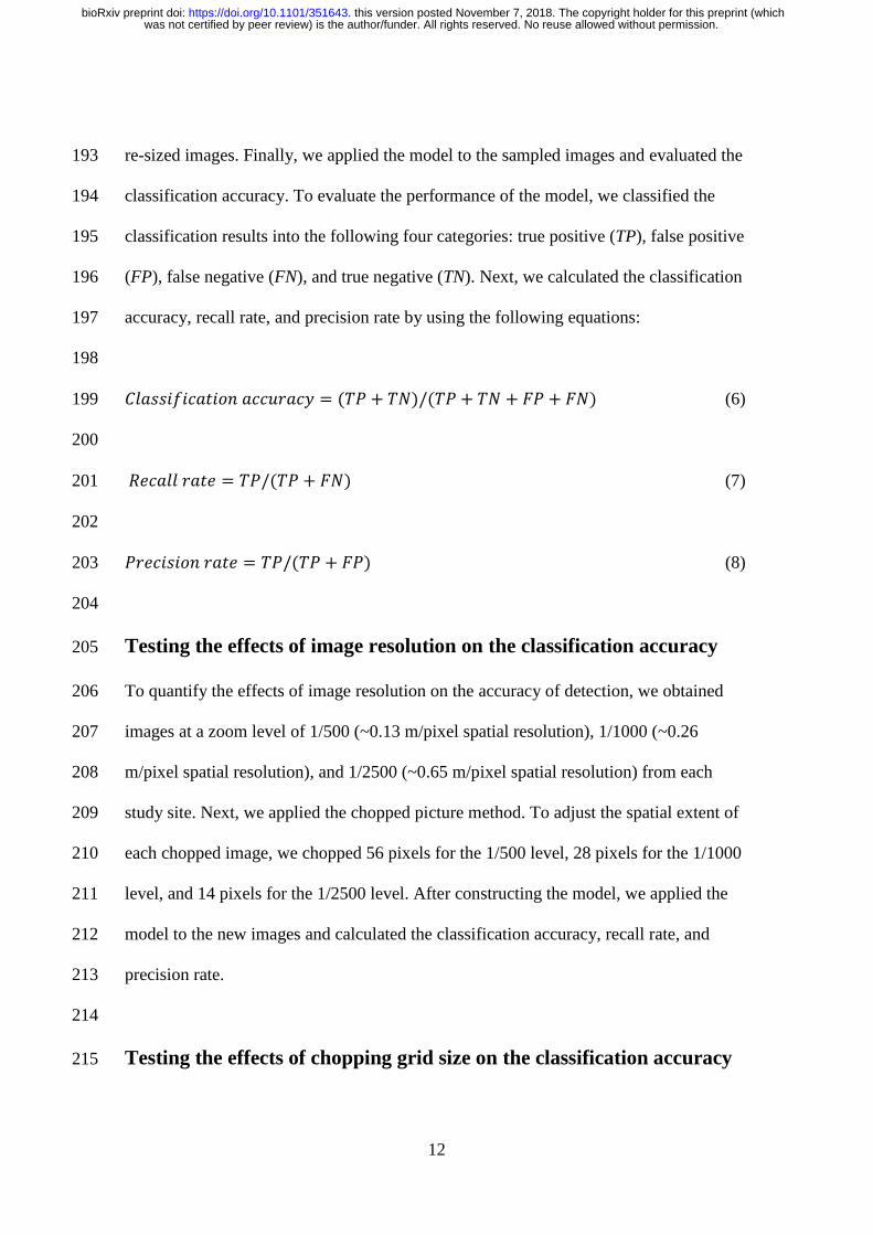
re-sized images. Finally, we applied the model to the sampled images and evaluated the 193

classification accuracy. To evaluate the performance of the model, we classified the 194

classification results into the following four categories: true positive (TP), false positive 195

(FP), false negative (FN), and true negative (TN). Next, we calculated the classification 196

accuracy, recall rate, and precision rate by using the following equations: 197

198

𝐶𝑙𝑎𝑠𝑠𝑖𝑓𝑖𝑐𝑎𝑡𝑖𝑜𝑛 𝑎𝑐𝑐𝑢𝑟𝑎𝑐𝑦 = (𝑇𝑃 + 𝑇𝑁)/(𝑇𝑃 + 𝑇𝑁 + 𝐹𝑃 + 𝐹𝑁) (6) 199

200

𝑅𝑒𝑐𝑎𝑙𝑙 𝑟𝑎𝑡𝑒 = 𝑇𝑃/(𝑇𝑃 + 𝐹𝑁) (7) 201

202

𝑃𝑟𝑒𝑐𝑖𝑠𝑖𝑜𝑛 𝑟𝑎𝑡𝑒 = 𝑇𝑃/(𝑇𝑃 + 𝐹𝑃) (8) 203

204

Testing the effects of image resolution on the classification accuracy 205

To quantify the effects of image resolution on the accuracy of detection, we obtained 206

images at a zoom level of 1/500 (~0.13 m/pixel spatial resolution), 1/1000 (~0.26 207

m/pixel spatial resolution), and 1/2500 (~0.65 m/pixel spatial resolution) from each 208

study site. Next, we applied the chopped picture method. To adjust the spatial extent of 209

each chopped image, we chopped 56 pixels for the 1/500 level, 28 pixels for the 1/1000 210

level, and 14 pixels for the 1/2500 level. After constructing the model, we applied the 211

model to the new images and calculated the classification accuracy, recall rate, and 212

precision rate. 213

214

Testing the effects of chopping grid size on the classification accuracy 215


https://doi.org/10.1101/351643

13

To quantify the effects of the spatial extent of the chopping grid on the accuracy of 216

detection, we chopped the 1/500 images at each study site for three types of pixel sizes 217

(84, 56, 28). After constructing the model, we applied the model to new images and 218

calculated the classification accuracy, recall rate, and precision rate. 219

220

Transferability test 221

Given the large amount of variation in the visual appearance of bamboo forest across 222

different cities, it is of interest to study to what extent a model learned on one 223

geographical location can be applied to a different geographical location. As such, we 224

performed experiments in which we trained a model for one (or more) cities, and then, 225

we applied the model to a different set of cities. Performance of the model was 226

evaluated by the classification accuracy, recall rate, and precision rate. 227

228

RESULTS 229

Fluctuation of accuracy and loss during the learning epochs 230

The accuracy for classifying the validation data of the final layer ranged from 94% to 231

99%. Loss values for the validation data ranged from 0.008 to 0.214 (Figure 4). Values 232

of accuracy increased and loss decreased following the learning epochs (Figure 4). 233

These results suggest the all of the models were not overfit to the datasets and 234

successfully learned the features of chopped pictures. 235


https://doi.org/10.1101/351643

14

236

FIGURE 4 Accuracy and loss (val) of the model at each learning epoch. 237

238

Effects of image resolution on the classification accuracy 239

The classification accuracy ranged from 76% to 97% (Figure 5a). The recall rate and 240

precision rate for bamboo forest ranged 52% to 96% and 91% to 99%, respectively 241

(Figure 5b, d). The recall rate and precision rate for objects other than bamboo forest 242

ranged from 92% to 99% and 67% to 96%, respectively (Figure 5c, e). The recall rate 243

for bamboo forest declined following the decline in the image resolution, and it declined 244


https://doi.org/10.1101/351643

15

dramatically when we used the 1/2500 level (~0.65 m/pixel spatial resolution) (Figure 245

5a). 246

247

FIGURE 5 Sensitivity of the image scale versus the test accuracy. 248

249

Effects of chopping grid size on the classification accuracy 250

The classification accuracy ranged from 85% to 96% (Figure 6a). The recall rate and 251

precision rate for bamboo forest ranged from 79% to 99% and 89% to 98%, respectively 252

(Figure 6b, d). The recall rate and precision rate for objects other than bamboo forest 253


https://doi.org/10.1101/351643

16

ranged from 88% to 98% and 79% to 99%, respectively (Figure 6c, e). The 254

intermediate-sized images (56 pixel) showed the highest classification accuracy at all 255

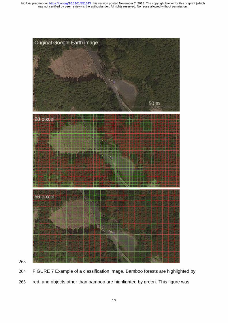
sites (Figure 6a). An example of a classification image is shown in Figure 7.256

257

FIGURE 6 Sensitivity of the pixel size versus the test accuracy. 258

259

260

261

262


https://doi.org/10.1101/351643

17

263

FIGURE 7 Example of a classification image. Bamboo forests are highlighted by 264

red, and objects other than bamboo are highlighted by green. This figure was 265


https://doi.org/10.1101/351643

18

generated using data from Google Earth image (Image data: ©2018 266

CNES/Airbus & Digital Globe). 267

268

Transferability and classification performance 269

In general, performance was poor when training on samples from a given city and 270

testing on samples from a different city (Figure 8a). When the model that was trained by 271

the images of Isumi city was applied to the other cities, the recall rate was the worst 272

(Figure 8b). Conversely, the model that was trained by the images of Sanyo city showed 273

the highest recall rate (Figure 8b). We noticed that a more diverse set (all) did not yield 274

a better performance when applied at different locations than the models trained on 275

individual cities (Figure 8). 276


https://doi.org/10.1101/351643

19

277

FIGURE 8 Transferability of the models learned at one location and applied at 278

another. 279

280

DISCUSSION 281

In this paper, we demonstrated that the chopped picture method and CNN could 282

accurately detect bamboo forest in Google Earth imagery (see Figure 7). Recent 283

research has shown that the deep learning technique is applicable to plant science 284

research 8-11, 21,22; however, applications of DA in plant science have been mainly 285

restricted to photographs taken indoors, and applications to plants in the aerial 286


https://doi.org/10.1101/351643

20

photographs are still limited11. To the best of our knowledge, this is the first study to 287

successfully identify plant communities automatically from Google Earth imagery. 288

Classifying vegetation from remote sensing images generally suffers from 289

several problems, e.g., it can be difficult to establish a specific pattern for each species, 290

given the high intraclass variance, and also to distinguish between different species, 291

given the interclass similarity of distinct species12, 23. So far, it is generally been difficult 292

to detect ambiguous objects such as vegetation, but our results showed good 293

performance during the detection of bamboo forest from Google Earth images by using 294

the chopped picture method even though we employed the most classical CNN (LeNet). 295

Our results highlight that the chopped picture method and CNN would be a powerful 296

method for high accuracy automated bamboo forest detection and vegetation mapping 297

(see Figure 9). 298


https://doi.org/10.1101/351643

21

299

FIGURE 9 Example of applying the model to the wide area of Ide city. The left 300

image is the original Google Earth image, and the right image shows the results 301

of bamboo forest detection. Bamboo forests are highlighted by red, and objects 302

other than bamboo are highlighted by green. This figure was generated using 303

data from Google Earth image (Image data: ©2018 CNES/Airbus & Digital 304

Globe). 305


https://doi.org/10.1101/351643

22

306

307

Effects of image resolution on the classification accuracy 308

Our results indicate that the image resolution strongly affects the identification accuracy 309

(Figure 4). As the resolution rate decreased, performance of the model also declined 310

(Figure 4). 311

Especially in the 1/2500 imagery, the recall rate for bamboo forest of Sanyo-312

Onoda and Isumi city declined to 53% and 64%, respectively (Figure 4b). In contrast, 313

the precision rate for bamboo forest increased as the resolution decreased (Figure 4d). 314

This result means that as the resolution decreases, the model overlooks many bamboo 315

forests; thus, when the image resolution is low, it is difficult to learn the features of the 316

object. This result also suggests that in the deep learning model, misidentification due to 317

false negatives is more likely to occur than misidentification due to false positive as the 318

image resolution declines. 319

320

Effects of chopping grid size on the classification accuracy 321

Our results indicate that the chopping grid size also affects the performance of the 322

model. The classification accuracy was the highest at the medium pixel size (56 × 56 323

pixels; Figure 5a). In contrast to the effects of image resolution, the recall rate and 324

precision rate for bamboo forest was also the highest at the medium pixel size except for 325

the recall rate at Ide city (Figure 5b, d). 326

This result means that if the grid size is inappropriate, both false positives and false 327

negatives will increase. 328


https://doi.org/10.1101/351643

23

Increases of the chopping grid size will cause an increase in the number of 329

chopped pictures in which objects other than bamboo and bamboo are mixed. In this 330

paper, because we evaluated the performance of the model by using images that were 331

uniformly covered by bamboo forest or objects other than bamboo forest, the effects of 332

imagery consisting of mixed objects on the classification accuracy could not be 333

evaluated. Evaluation of the classification accuracy for such images will take place in 334

future research. 335

336

Transferability among the models 337

Results for the transferability tests showed that transferability was generally poor and 338

suggest that the spatial extent of acquisition of training data strongly influences the 339

classification accuracy (Figure 8). The model trained by Sanyo-Onoda city images 340

yielded high recall rates for the images taken at all of the study sites, but the precision 341

rate was lower than that of the other models (Figure 8b, c). This means that the model 342

trained by Sanyo-Onoda city images tends to make false positive mistakes. 343

Interestingly, transferability was not found to be related to the distance among the study 344

sites (Figure 8). This result indicates that classification accuracy across the model 345

reflects the conditions at the local scale such as the climate at the time when the image 346

was taken. Additionally, even when we applied a model that learned from all training 347

images (all), the performance of the model was not as good as when the training data 348

were obtained within the same city. The same tendencies have been reported in studies 349

that classified land use by using deep learning 24. This may suggest that increasing the 350

number of training data may also lead to a decrease in the identification accuracy, and it 351

may be difficult to construct an identification model applicable to a broad area. 352


https://doi.org/10.1101/351643

24

353

Conclusions and future directions 354

Our results show that the deep learning model presented here can detect bamboo forest 355

from Google Earth images accurately. Our results also suggest that deep learning and 356

the chopped picture method would be a powerful tool for high accuracy automated 357

vegetation mapping and may offer great potential for reducing the effort and costs 358

required for vegetation mapping as well as improving the current status of monitoring 359

the distribution of bamboo. Recently, bamboo expansion has become an important 360

problem in Japan because of its invasiveness17. While some research has analyzed the 361

bamboo forest distribution probability on a national scale25, 26, monitoring of bamboo 362

expansion is still a challenging problem because of labor requirements. Our approach 363

could potentially lead to the creation of a semi or even fully automated system for the 364

monitoring of bamboo expansion. 365

Our results also suggest that the identification accuracy depends on the image 366

resolution and chopping grid size. Especially, the spatial resolution of training data 367

strongly affects the model performance. Generally, satellite-based remote sensing has 368

been widely studied and applied but suffers from insufficient information due to low 369

resolution images or inaccurate information due to local weather conditions27. Our 370

results also show that the performance of the model can be greatly influenced by the 371

spatial extent of the acquired training data and a model learned on one geographical 372

location is difficult to apply to a different geographical location. It remains a future task 373

to develop a model that can be applied over a wide spatial scale. 374

375

ACKNOWLEDGEMENTS 376


https://doi.org/10.1101/351643

25

This work was supported by JST PRESTO, Japan (Grant No. JPMJPR15O1). 377

378


https://doi.org/10.1101/351643

26

Author Contributions 379

S. W designed the research based on discussion with T. I. S. W and K. S 380

conducted research. S. W and T. I wrote the manuscript. 381

382

Competing interests 383

The authors declare no competing interests. 384

385

386

387


https://doi.org/10.1101/351643

27

REFERENCES 388

1. Franklin, J. Mapping Species Distributions: Spatial Inference and Prediction. 389

(Cambridge University Press, 2009). 390

2. Xie, Y., Sha, Z., & Yu, M. Remote sensing imagery in vegetation mapping: a review. 391

Journal of Plant Ecology, 1, 9–23. doi: 10.1093/jpe/rtm005 (2008). 392

3. Hearst, M. A., Dumais, S. T., Osuna, E., Platt, J., & Schölkopf, B. Support vector 393

machines. IEEE Intelligent Systems and their Applications, 13, 18–28. doi: 394

10.1109/5254. 708428 (1998). 395

4. Bengio, Y. Learning deep architectures for AI. Foundations and Trends in Machine 396

Learning, 2, 1–127 (2009). 397

5. Goodfellow, I., Bengio, Y. & Courville, A. Deep Learning (MIT press, 2016) 398

6. Karpathy, A., Toderici, G., Shetty, S., Leung, T., Sukthankar, R., & Fei-Fei, L. 399

Large-scale video classification with convolutional neural networks. Proceedings of 400

the IEEE Conference on Computer Vision and Pattern Recognition (Columbus), 401

1725–1732 (2014). 402

7. Yosinski, J., Clune, J., Bengio, Y., & Lipson, H. How transferable are features in 403

deep neural networks? Advances in Neural Information Processing Systems 404

(Montreal), 3320–3328 (2014). 405

8. Mohanty, S. P., Hughes, D. P., & Salathé, M. Using deep learning for image-based 406

plant disease detection. Frontiers in Plant Science, 7, 1419. doi: 407

10.3389/fpls.2016.01419 (2016). 408

9. Ramcharan, A., Baranowski, K., McCloskey, P., Ahamed, B., Legg, J., & Hughes, 409

D. Deep learning for image-based cassava disease detection. Frontiers in Plant 410

Science, 8, 1852 (2017). 411


https://doi.org/10.1101/351643

28

10. Carranza-Rojas, J., Goeau, H., Bonnet, P., Mata-Montero, E., & Joly, A. Going 412

deeper in the automated identification of Herbarium specimens. BMC Evolutionary 413

Biology, 17, 181 (2017). 414

11. Nogueira, K., Penatti, O. A. B., & Dos Santos, J. A. Towards better exploiting 415

convolutional neural networks for remote sensing scene classification. Pattern 416

Recognition, 61, 539–556 (2017). 417

12. Zhu, X.X., Tuia, D., Mou, L., Xia, G.S., Zhang, L., & Xu, F. Deep Learning in 418

Remote Sensing: A Comprehensive Review and List of Resources. IEEE Geosci. 419

Remote Sens. Mag, 5, 8–36 (2017). 420

13. Guirado, E., Tabik, S., Alcaraz-Segura, D., Cabello, J., & Herrera, F. Deep-learning 421

Versus OBIA for Scattered Shrub Detection with Google Earth Imagery: Ziziphus 422

lotus as Case Study. Remote Sensing, 9, 1220. doi: 10.3390/rs9121220 (2017). 423

14. Ise, T., Minagawa, M., & Onishi, M. Classifying 3 moss species by deep learning, 424

using the “chopped picture” method. Open Journal of Ecology, 8, 166–173 (2018). 425

15. Nakashima, A. The present situation of the bamboo forests management in the 426

suburbs: A case study of the bamboo shoot producing districts in the suburbs of 427

Kyoto City. Applied Forest Science, 10, 1–7 (in Japanese with English abstract) 428

(2001). 429

16. Nishikawa, R., Murakami, T., Yoshida, S., Mitsuda, Y., Nagashima, K., & Mizoue, 430

N. Characteristic of temporal range shifts of bamboo stands according to adjacent 431

landcover type. Journal of the Japanese Forestry Society, 87, 402–409 (in Japanese 432

with English abstract) (2005). 433


https://doi.org/10.1101/351643

29

17. Okutomi, K., Shinoda, S., & Fukuda, H. Causal analysis of the invasion of broad-434

leaved forest by bamboo in Japan. Journal of Vegetation Science, 7, 723–728 435

(1996). 436

18. Suzuki, S. Chronological location analyses of giant bamboo (Phyllostachys 437

pubescens) groves and their invasive expansion in a satoyama landscape area, 438

western Japan. Plant Species Biology, 30, 63–71 (2015). 439

19. NVIDIA NVIDIA deep learning gpu training system. 440

https://developer.nvidia.com/digits. Accessed June 1, 2018 (2016). 441

20. LeCun, Y. L., Bottou, L., Bengio, Y., & Haffner, P. Gradient-based learning applied 442

to document recognition. Proceedings of the IEEE, 86, 2278–2324. doi: 443

10.1109/5.726791 (1998). 444

21. Wäldchen, J., Rzanny, M., Seeland, M., & Mäder, P. Automated plant species 445

identification—Trends and future directions. PLoS Computational Biology, 14(4), 446

e1005993. https://doi.org/10.1371/journal.pcbi.1005993 (2018). 447

22. Wäldchen, J., & Mäder, P. Machine learning for image based species identification. 448

Methods Ecol Evol. 2018, 1–10. doi: 10.1111/2041-210X.13075 (2018). 449

23. Rocchini, D., Foody, G. M., Nagendra, H. et al. Uncertainty in ecosystem mapping 450

by remote sensing. Computers and Geosciences, 50, 128–135 (2013). 451

24. Albert, A., Kaur, J., & Gonzalez, M. Using convolutional networks and satellite 452

imagery to identify patterns in urban environments at a large scale. arXiv preprint, 453

arXiv:1704.02965 (2017). 454

25. Someya, T., Takemura, S., Miyamoto, S., & Kamada, M. Predictions of bamboo 455

forest distribution and associated environmental factors using natural environmental 456


https://doi.org/10.1101/351643

30

information GIS and digital national land information in Japan. Keikanseitaigaku 457

[Landscape Ecology], 15, 41–54 (in Japanese with English abstract) (2010). 458

26. Takano, K. T., Hibino, K., Numata, A., Oguro, M., Aiba, M., Shiogama, H., 459

Takayasu, I., & Nakashizuka, T. Detecting latitudinal and altitudinal expansion of 460

invasive bamboo Phyllostachys edulis and Phyllostachys bambusoides (Poaceae) in 461

Japan to project potential habitats under 1.5°C–4.0°C global warming. Ecology and 462

Evolution, 7, 9848–9859 (2017). 463

27. Jones, H. G., & Vaughan, R. A. Remote Sensing of Vegetation: Principles 464

Techniques and Applications (Oxford University Press, 2010). 465

466

467

468

469

470

471

472

473

474


https://doi.org/10.1101/351643

Documents

Automatic vegetation identification in Google Earth images using a convolutional … · convolutional neural network: A case study for Japanese bamboo forests Shuntaro Watanabe 1,