Ing. Richard Schumi BSc

Automatic Test Case Generation from

Formal Models

to achieve the university degree of

MASTER'S THESIS

Master's degree programme: Computer Science

submitted to

Graz University of Technology

Univ.-Prof. Roderick Bloem, M.Sc. Ph.D.

Institute for Applied Information Processing and Communications Head: Univ.-Prof. Dipl-Ing. Dr.techn. Reinhard Posch

Diplom-Ingenieur

Supervisor

Second Supervisor Dipl.-Ing. Franz Röck

Graz, March 2015

AFFIDAVIT

I declare that I have authored this thesis independently, that I have not used other

than the declared sources/resources, and that I have explicitly indicated all ma-

terial which has been quoted either literally or by content from the sources used.

The text document uploaded to TUGRAZonline is identical to the present master‘s

thesis dissertation.

Date Signature

Abstract

Testing is a very important measure to achieve software with high qual-ity and to comply with certain security requirements for security-criticalsystems. It also is very important to find ways to reduce the time consump-tion for testing, because thereby the development costs can be significantlyreduced. Therefore, it is advantageous to use automation.

In this thesis we describe the development of a tool for automatic test casegeneration from formal (NuSMV) models. This tool uses graph-based andlogic-based coverage criteria for the generation of trap properties, whichare given to a model checker in order to produce abstract test cases. First,we evaluate and compare different graph-based and logic-based coveragecriteria. Then, we explain the development process, the structure of the tooland important components like model parsing, counter example generationwith a model checker and test adaption.

Furthermore, we show a case study, where the tool is applied to a realworld project, in order to see if it is practicable. In this case study the modelreflects the behavior of a cache system and it reproduces the actions that arenecessary for the cache access. We show how the counter examples from themodel checker are used as abstract test cases for several systems under testand how the test adaption can be accomplished with different abstractionlevels.

Then, we analyze if the generated test cases have sufficient coverage on themodel and the system under test and if it is possible to find any errors orspecification problems.

iii

Zusammenfassung

Testen ist eine wichtige Maßnahme, um Software mit hoher Qualitat zuentwickeln und um bestimmte Sicherheitsanforderungen bei sicherheitskri-tischen Systemen zu erfullen. Es ist auch sehr wichtig, Wege zu finden,um den Zeitaufwand furs Testen zu reduzieren, weil dadurch die Entwick-lungskosten erheblich gesenkt werden konnen. Daher ist es wesentlich,Automatisierung zu verwenden.

In dieser Arbeit wird die Entwicklung eines Tools zur automatischen Test-fallgenerierung aus formalen (NuSMV) Modellen gezeigt. Das Tool verwen-det graphenbasierte und logikbasierte Testabdeckungskriterien um TrapProperties zu erzeugen, welche dann einen Model Checker ubergebenwerden, um abstrakte Testfalle zu erzeugen. Erst werden verschiedeneTestabdeckungskriterien ausgewertet und verglichen. Dann werden der En-twicklungsprozess und die Struktur des Tools beschrieben und wichtigeKomponenten, wie Modell-Parsing, Gegenbeispielgenerierung mit einemModel-Checker und Testadaption, werden erlautert.

Des Weiteren wird eine Fallstudie durchgefuhrt, bei welcher das Tool furein richtiges Projekt verwendet wird, um zu uberprufen, ob es praktischverwendbar ist. In dieser Fallstudie bildet das Modell das Veralten einesCache-Systems ab und die notigen Aktionen fur den Cache-Zugriff werdenreproduziert. Es wird gezeigt, wie die Gegenbeispiele vom Model-Checkerals abstrakte Testfalle auf verschiedenen zu testenden Systemen verwendetwerden, und wie die Testadaption mit unterschiedlichen Abstraktionsebenendurchgefuhrt werden kann.

Danach wird untersucht, ob die generierten Testfalle eine ausreichendeTestabdeckung auf dem Modell und zu testenden System haben, und eswird uberpruft, ob es moglich ist irgendwelche Fehler oder Spezifikations-abweichungen, zu finden.

iv

Contents

Abstract iii

1 Introduction 11.1 Background . . . . . . . . . . . . . . . . . . . . . . . . . . . . . 1

1.2 Problem Description . . . . . . . . . . . . . . . . . . . . . . . . 3

1.3 Solution . . . . . . . . . . . . . . . . . . . . . . . . . . . . . . . 4

1.4 Overview . . . . . . . . . . . . . . . . . . . . . . . . . . . . . . . 8

2 Basics 102.1 Temporal Logic . . . . . . . . . . . . . . . . . . . . . . . . . . . 10

2.1.1 LTL . . . . . . . . . . . . . . . . . . . . . . . . . . . . . . 10

2.2 Trap Properties . . . . . . . . . . . . . . . . . . . . . . . . . . . 11

2.3 Test Case Concretization and Test Adapter . . . . . . . . . . . 12

2.4 NuSMV . . . . . . . . . . . . . . . . . . . . . . . . . . . . . . . . 13

2.5 NuSMV Model . . . . . . . . . . . . . . . . . . . . . . . . . . . 13

2.6 Graph-based Coverage . . . . . . . . . . . . . . . . . . . . . . . 14

2.6.1 Node Coverage . . . . . . . . . . . . . . . . . . . . . . . 16

2.6.2 Edge Coverage . . . . . . . . . . . . . . . . . . . . . . . 16

2.6.3 Path Coverage . . . . . . . . . . . . . . . . . . . . . . . . 17

2.7 Logic-based Coverage . . . . . . . . . . . . . . . . . . . . . . . 19

2.7.1 Predicate Coverage . . . . . . . . . . . . . . . . . . . . . 19

2.7.2 Clause Coverage (CC) . . . . . . . . . . . . . . . . . . . 20

2.7.3 Combinatorial Coverage (CoC) . . . . . . . . . . . . . . 20

2.7.4 Active Clause Coverage (ACC) . . . . . . . . . . . . . . 21

2.7.5 Correlated Active Clause Coverage (CACC) . . . . . . 22

2.7.6 Restricted Active Clause Coverage (RACC) . . . . . . . 23

2.7.7 RACC versus CACC . . . . . . . . . . . . . . . . . . . . 23

3 Related work 25

v

Contents

4 Combination Method for Coverage Criteria 274.1 Combination of Edge Coverage with CACC . . . . . . . . . . 27

4.2 Combination of Path Coverage with CACC . . . . . . . . . . . 28

5 Tool Development 305.1 Component Structure . . . . . . . . . . . . . . . . . . . . . . . . 30

5.2 Model Parsing . . . . . . . . . . . . . . . . . . . . . . . . . . . . 31

5.2.1 Xtext . . . . . . . . . . . . . . . . . . . . . . . . . . . . . 32

5.2.2 Conversion of the Parsed Object Structure . . . . . . . 32

5.2.3 Parsed Model Structure . . . . . . . . . . . . . . . . . . 32

5.3 Model Visualization . . . . . . . . . . . . . . . . . . . . . . . . 33

5.4 Test Case Generation . . . . . . . . . . . . . . . . . . . . . . . . 35

5.4.1 Trap Property Generation . . . . . . . . . . . . . . . . . 36

5.4.2 Counter Example Generation . . . . . . . . . . . . . . . 37

5.5 Implemented Coverage Criteria . . . . . . . . . . . . . . . . . . 39

5.5.1 Graph-based Coverage Criteria . . . . . . . . . . . . . . 39

5.5.2 Combination of Graph-based Coverage with CACC . . 40

5.6 Configuration Options . . . . . . . . . . . . . . . . . . . . . . . 42

5.7 Additional Features . . . . . . . . . . . . . . . . . . . . . . . . . 43

5.8 Known Limitations . . . . . . . . . . . . . . . . . . . . . . . . . 47

5.9 Define Restriction . . . . . . . . . . . . . . . . . . . . . . . . . . 47

6 Tool Evaluation 496.1 Triangle Example . . . . . . . . . . . . . . . . . . . . . . . . . . 49

6.1.1 Functional Description . . . . . . . . . . . . . . . . . . . 50

6.1.2 SUT . . . . . . . . . . . . . . . . . . . . . . . . . . . . . . 50

6.1.3 Graphical Representation . . . . . . . . . . . . . . . . . 52

6.1.4 Test Adapter . . . . . . . . . . . . . . . . . . . . . . . . . 53

6.1.5 Results . . . . . . . . . . . . . . . . . . . . . . . . . . . . 56

6.2 Car Alarm Example . . . . . . . . . . . . . . . . . . . . . . . . . 58

6.2.1 Functional Description . . . . . . . . . . . . . . . . . . . 58

6.2.2 SUT . . . . . . . . . . . . . . . . . . . . . . . . . . . . . . 60

6.2.3 Graphical Representation . . . . . . . . . . . . . . . . . 62

6.2.4 Test Adaptation . . . . . . . . . . . . . . . . . . . . . . . 64

6.2.5 Results . . . . . . . . . . . . . . . . . . . . . . . . . . . . 64

vi

Contents

7 Case Study 687.1 SUT . . . . . . . . . . . . . . . . . . . . . . . . . . . . . . . . . . 68

7.2 Model Description . . . . . . . . . . . . . . . . . . . . . . . . . 69

7.3 Test Adapter . . . . . . . . . . . . . . . . . . . . . . . . . . . . . 73

7.4 Results . . . . . . . . . . . . . . . . . . . . . . . . . . . . . . . . 74

8 Outlook 78

9 Conclusion 80

Bibliography 84

vii

1 Introduction

1.1 Background

Software testing is a very important part of software engineering. Sometimesthe time consumption for testing can be the biggest part of the softwaredevelopment process. The purpose of testing is to achieve software with highquality, to detect defects and to ensure that requirements and specificationsare satisfied [26].

Software testing approaches can be categorized according to the knowledgeabout the system under test (SUT). Black box testing needs no knowledgeabout the internal structure of the SUT. It is considered as a black boxand only the inputs and outputs are known. White box testing, which issometimes also called structural testing, is a technique that inspects theinternal structure of a system. The source code or other internal componentsare considered when the tests are created. A combination of both approachesis called gray box testing, which for example is used when only limitedinternal information is considered [11, p.7].

Model-based testing is a form of black box software or system testing. Ituses an abstract model respectively formal specification of the behavior ofthe SUT and derives test cases from it. This model reflects certain states ofthe system, particular actions and decisions that lead to other states [30].

A model checker is a tool that takes a formal model in the form of a finitestate machine (FSM) and a specification or property in the form of a formulaas input and automatically checks if the model meets the specification. Whenthe model does not meet the specification, a counter example is produced.The counter example is in the form of a trace and it shows how the propertyis violated on the model. This trace can be used as an abstract test case and

1

1 Introduction

a test adapter executes it as concrete test case on the SUT. In this thesistrap properties are formulated with LTL. Linear temporal logic (LTL) is anextended version of classical logic and includes the classical logic operatorsfor negation, implication, conjunction, disjunction and additionally alsosome special operators that can reflect the temporal connection betweenevents or states [15, p. 2ff.], [20].

There are several assumptions on which model-based testing is based: Theassumption that an adequate model exists for a SUT. This assumption dealswith the abstraction level of the model. When the model is too abstract, thenit may include too less details and so the coverage on the SUT could betoo low. When it is too precise, it may be too complex and the validationcan be difficult. Therefore, it is important to find a good balance betweenabstraction and precision. Another assumption is that if an adequate modelis found, then effective model-based testing is possible and it is possible toreveal errors in the SUT. Furthermore, we assume that a high coverage onthe model also leads to high coverage on the SUT, when an adequate modelwith a good abstraction level was found [29], [30].

Coverage criteria are important to ensure that test cases inspect certainmodel parts. Especially for security-critical systems it is important to en-sure that there are no vulnerabilities that could be used from attackers tocompromise the system. A model of security-critical system component canhelp to find weak points because it can be used to find deviations fromthe specification. These deviations might cause potential vulnerabilities.In order to find these deviations it is important to apply certain coveragecriteria.

When it comes to testing, another important topic is automation. Test casegeneration is a complicated task, which requires experienced tester andmuch time. When it is done manually it is difficult to ensure that the testsmeet all requirements, are consistent and fulfill a certain coverage criterion.For example it would be difficult to ensure that all paths of a certain lengthare covered.

Automatic test case generation has many benefits. It can produce a highnumber of test cases that are reliable and have high quality in a shorttime [27]. It is useful in order to save time and costs and is also usablefrom users with limited experience in this area. Furthermore, it is less error

2

1 Introduction

prone, because an automated system does not forget to cover some modelcomponents.

1.2 Problem Description

Security-critical systems can have certain requirements with regard to test-ing. For example for some high risk areas like safety critical software inaircraft it is necessary to ensure that a specific test coverage criterion isachieved, in order to comply with security standards [28]. For other areas itis important to ensure that there are no vulnerabilities that could be usedfrom attackers to compromise a system. It is necessary that the generatedtest cases cover certain model parts. For example, it could be required thatall transitions of the model are visited with at least one test case. It is alsoimportant that the number of test cases does not become too large, so that itis still manageable.

There are already some approaches that deal with coverage criteria and havea focus on graph-based and logic-based coverage methods. For exampleFraser, Wotawa, and Ammann [12] and Ammann, Offutt, and Xu [2] wroteabout this topic and gave an overview of specific coverage criteria, butthey showed no practical applications and also no combined approachesfor graph-based and logic-based coverage criteria. Although Weißleder [32]presented a combined approach, it was only for very specific model typesand this approach is not so easy to generalize for other models.

So the problem is that mostly only theoretical approaches for graph-basedand logic-based coverage criteria exist and hardly any practical imple-mentations, evaluations and approaches with combinations exist. The onlyapproaches with a combined method, we could find were from Offutt et al.[22], Weißleder [32] and Ammann, Offutt, and Xu [2], but they only showedone combination method.

To the best of our knowledge, we could not find any work that includesdifferent combination methods for graph-based and logic-based coveragecriteria.

3

1 Introduction

In this thesis we want to challenge this problem and find combinations fordifferent graph-based and logic-based coverage criteria, which still producea manageable number of test cases. Furthermore, we want to create anautomatic test case generation tool that implements these combined coveragecriteria and apply it to real world projects and we want to demonstrate thatthe test case generation with these combined coverage criteria can achieve ahigh instruction and branch coverage on the SUTs.

1.3 Solution

Initially we studied the field of model-based testing with a focus on coveragecriteria. Then, we analyzed graph-based coverage criteria and after thatlogic-based coverage criteria.

Graph-based coverage criteria are coverage metrics that require test casesto regard certain graph components from the models. The most commonones are node coverage, edge coverage and path coverage. Node coverageis a very simple form of coverage. In order to fulfill node coverage it isonly necessary that every node in the model is visited at least once. Edgecoverage demands that all edges between each node pair are visited at leastonce. Path coverage is similar to edge coverage, but it does not only consideredges between node pairs, but also connected edges, which form a path. Incontrast to node and edge coverage, complete path coverage is not possiblefor models with loops, but it is possible to fulfill path coverage for paths ofa certain length [2], [12].

Logic-based coverage criteria are applied to logical expressions. In contractto graph-based coverage criteria they deal with predicates and clauses. Inthis thesis they are applied to edge conditions or guards. Very commonlogic-based coverage criteria are predicate coverage, clause coverage andactive clause coverage. Predicate coverage is relatively simple, it requiresthat each predicate has to evaluate to true and false at least one time. Clausecoverage is accomplished when each clause evaluates to true and false atleast once. For Active Clause Coverage (ACC) it is required to test eachclause under circumstances where it has an influence on the predicate value.Correlated Active Clause Coverage (CACC) is also referred to as masking

4

1 Introduction

Modified Condition Decision Coverage (MCDC) and it is the most commonversion of ACC. MCDC is a very common code coverage criterion [2]. Theseterms will be defined in Section 2.7.

In this thesis we apply coverage criteria by using trap properties and anabstract model of the system. Trap properties are formulas that formulate aknown property of the model in negated form. They are used to generatecounter examples that verify a certain property of a model and they canbe used as abstract test cases by a test adapter. In order to produce thesecounter examples, a model checker is needed.

Counter examples generated by a model checker have the advantage thatthey are in an abstract form and can be used very flexible for differentsystems, without the need to generate them again. They are representedas traces and are a sequence of states that shows a state change when thevalue of certain variables changes. For the test adaptation the traces areparsed and converted into variable assignment maps. Each of these tracesrepresents a test case or a sequence of test cases depending on the systemabstraction.

The test adaption with these abstract test cases is also possible in differentways. For example they can be used to directly interact with the SUTand give it inputs and compare the output. Another way is to generatesource code for test function calls with test data and the expected output asarguments. However, the abstract test cases could be used for other adaptionconcepts.

The coverage criteria were implemented by a tool that automatically gen-erates test cases according to a selected criterion. This tool uses a NuSMVmodel file of the SUT as input and generates test cases as output, whichfulfill a certain selected coverage criterion. NuSMV and NuSMV modelsare defined in Section 2.4 and Section 2.5. The tool supports the generationof test cases with different coverage criteria, so that a comparison can bedone.

The structure of the tool was made flexible in order to make it easy toinclude new coverage criteria. It consists of several components. The firstcomponent is the model parser, which uses a NuSMV file and makes anobject representation, which can include one or multiple graphs. This object

5

1 Introduction

Figure 1.1: Schematic overview of the main tool components and their correlation.

representation is then used by the test case generator component, whichuses it to traverse over the graphs and creates trap properties according to acertain selected coverage criterion.

When the trap properties are finished, they are used as input for a NuSMVprocess, which creates counter examples traces that then can be used as testcases by a test adapter.

Figure 1.1 shows an overview of the program components and how theyinteract.

In order to develop combination methods for graph-based and logic-basedcoverage we applied CACC to edge coverage and path coverage. For CACCwe used a given external tool [5] that generates variable assignments for

6

1 Introduction

CACC. The edge conditions are used as input for this tool and the output aredifferent assignment sets. Each of these sets is used in combination with thetrap property of the associated edge, both for edge and path coverage. Theoriginal trap property formula is combined with this generated assignmentsand so a new trap property is formed that considers one case for CACC.

We made several small conceptual examples in order to test the functionalityof the developed tool and to show how it works. They were also usedto demonstrate, how the generated counter examples could be parsedand then executed on the SUT. We used real implementations in order toshow how the test adaption process works and we compared the differentcoverage criteria on the basis of instruction and branch coverage on theseimplementations.

One SUT that we used was for the triangle example as described in Sec-tion 6.1. This example could show that edge coverage could improve thecode coverage compared to node coverage and it also showed what tasks ofthe test generation process need the most execution time. Another examplewas the car alarm system as described in Section 6.1. It could illustrate thatthe combination of graph based coverage criteria with CACC can improvethe branch coverage. This improvement could be shown for edge coverageand for path coverage.

In order to check if the developed tool is usable for real world examples, wemade a case study. For this case study a model of a cache implementationwas developed by Franz Rock and Daniel Hein. The case study shouldanalyze what problems can occur, which coverage criteria are best suitablefor the given model, if there are certain limitations for the trap propertygeneration or any other issues. Furthermore, the performance data and testquality was measured.

As expected, the case study showed some problems. For example the size ofthe model and some additional model features, which were not consideredearlier, caused the necessity for some modifications to the model, to the tooland to the test adaption process. In the test adaption process the abstract testcases in the form of counter examples were parsed and converted to concretetest cases for the SUT. For the cache implementation the abstract counterexamples were used to generate source code in the form of function calls towrapper functions with test data as arguments. These wrapper functions

7

1 Introduction

were used to perform the test execution and to check if the expected cachecontent matches the actual cache content after the execution.

Another issue was the assignment generation with the CACC tool. Definerestrictions for certain variables caused assignments that were not appli-cable on the model. So CACC could not be applied to some problematicvariables, but simple graph-based coverage like edge coverage could beused as alternative. Details about the define restrictions can be found inSection 5.9.

For the given model from the case study edge coverage could reach the bestcoverage on the SUT with the least number of test cases. Edge coveragecombined with CACC could show the best coverage for most model parts,only for certain variables, simple edge coverage produced trap propertieswith a better model coverage. The model coverage was analyzed by visuallyhighlighting the covered model parts, when a valid trap property could beproduced. The coverage on the SUT was measured by line and the branchcoverage. For the involved functions line coverage of 89.52% and branchcoverage of 90.48% could be reached, only some conditions for error checkswere not covered. Moreover, an old version of the cache implementationwith a bug that was only found with a lot of manual effort was tested andthe bug could be found easily.

We showed that the developed tool is useful for real world examples. Fur-thermore, it provides the advantage that a lot of test cases can be generatedin a relatively short time, without the need to be expert for coverage criteriaand with little manual effort.

1.4 Overview

Chapter 2 describes background information for the research field. Temporallogic, trap properties, NuSMV, graph-based and logic-based coverage criteriaare described in detail.

In Chapter 3, the related work, which was used, is analyzed and com-pared.

8

1 Introduction

The combination methods for graph-based and logic-based coverage criteriaare shown in Chapter 4.

Chapter 5 describes how a tool was developed, how it is structured, how itcan be used and what features it provides. The development of the tool isexplained and also some limitations for the functionality are mentioned.

In Chapter 6, simple examples demonstrate how the tool can be used andhow the generated test cases can be applied to the SUT. The examplesalso were used for a first evaluation of the tool and in order to test if thegeneration of the test cases worked as expected.

The case study is shown in Chapter 7. It describes how the tool is used for areal practical example and the problems that occur. Also the quality of thegenerated test cases is measured and other results are shown.

Chapter 8 provides an outlook. It shows how the tool could be improved,what features could be added and how known limitations could be reduced.It also shows what other potential future research could be done. Finally, inChapter 9 there is the conclusion of the work, where the results of thesis aresummarized.

9

2 Basics

In this chapter we explained some basics that were necessary for the under-standing of the research field. First temporal logic, trap properties, NuSMVand NuSMV models are described. Then, different graph-based and logic-based coverage criteria are explained and compared.

2.1 Temporal Logic

The description in this section is based on the work from Lahtinen [20].Temporal logic is an extended version of classical logic, which supportsthe expression of a temporal order of states or events without the need toadd clock values. There are certain additional operators, which are used todescribe this order. There are different forms of temporal logics, which canbe distinguished by their time structure. However, only one of them wasused in this thesis and it is described in the following section. [20]

2.1.1 LTL

Linear temporal logic (LTL) as defined by [25] is a version of temporal logic.It includes the classical logic operators for negation, implication, conjunction,disjunction and additionally there are also some special operators that canreflect the temporal connection between states or events without clockvalues. LTL has linear time structure, which means that it can be used todefine formulas about the future of paths. The additional operators that LTLprovides are the following:

10

2 Basics

• X Next operator: The expression which follows after the operatorhas to be true in the next state.• G Globally operator: This operator requires that the expression,

which follows after it, has to be true on all following states in the path.• F Eventually or Finally operator: For this operator it is required that

the subsequent expression has to evaluate to true at any time of thepath in the future.• U Until operator: The expression on the left side of the operator

has to be true until the expression from the right side of the operatorbecomes true and it is also required that the right expression mustevaluate to true eventually.• R Release operator: Either the expression on the right side of the

operator has to be always true, or at least it has to be true until theexpression on the left side of the operator becomes true.

LTL formulas are structured as follows: The X, G and F operators are unary,so they require an expression that follows them. This expression can alsoinclude LTL operators. The U and R operators are binary and so they needan expression on the left and right side of them. Both expressions can alsoinclude LTL operators. The resulting formulas that can be built with theseoperators, are the following:

φ := true| f alse|φ ∨ φ|φ ∧ φ|¬φ|φ→ φ|

X φ|G φ|F φ|φ U φ|φ R φ

Although LTL has many application areas like definition of safety or livenessproperties, in this thesis LTL is essentially used for the definition of trapproperties. There are many examples in the following chapters, where LTLis applied in order to formulate trap properties [20], [18].

2.2 Trap Properties

Trap properties are formulas that formulate a known property of the modelin negated form. They are used to generate counter example that verify

11

2 Basics

this known property. For example a property could be that it is possible toreach a certain state eventually and the negation would be that it is globallynot possible to reach this state. The negation is needed in order to producethis counter example for the property, which needs to be checked. For thegeneration of the counter examples the trap properties are given to a modelchecker. A model checker is a tool that takes a formal model in the form ofa FSM and a specification or property in the form of a formula as input andautomatically checks if the model meets the specification. When the modeldoes not meet the specification, a counter example is produced. A counterexample is in the form of a trace that shows how the unnegated property isreached in the model. Additionally it can be used as an abstract test case.[15, p. 2ff.]

Trap properties should normally produce a counter example because theyare the negation of a known property of the model. However, in this thesiswe want to create trap property for expected properties and not for knownproperties because for the trap property generation we do not know allproperties precisely. (This is for example the case, when there are definerestrictions in the model as described in Section 5.9.) Hence, in this thesistrap properties are divided in valid and invalid types. A trap propertyis invalid, if it does not produce a counter example because it is true forthe specification, otherwise it is valid. These invalid trap properties arerecognized when they are presented to the model checker and then they aredismissed.

2.3 Test Case Concretization and Test Adapter

In this thesis, counter examples are in the form of traces that show asequence of variable assignments for the model variables. This assignmentsequence reveals how the given property becomes false for the model andit represent an abstract test sequence. This abstract test sequence can beconverted by a test adapter to one or more concrete test cases for the SUT.A test adapter is a tool that parses abstract test cases, makes a connectionwith a SUT and executes these parsed test cases on the SUT. It uses certain

12

2 Basics

variable assignments from the trace as inputs for the SUT and also asexpected outputs, which are compared with the real outputs of the SUT.

A concrete test case is an execution of the SUT with given inputs andexpected outputs. The set of all test cases for a specific coverage criterion iscalled a test suite.

2.4 NuSMV

NuSMV is a new symbolic model checker (SMV) that allows model checkingfor temporal logic defined in LTL and Computational Tree Logic (CTL) andit has a robust and highly modular implementation that is well documented.Furthermore, there is the NuSMV input language that allows the descriptionof models in the form of FSMs and to define model specification with LTLand CTL Formulas. [9]

2.5 NuSMV Model

The NuSMV input language can be used to define FSMs. The FSM structurecan be descried with a tuple M = 〈 Q0, (Q, E), P〉P : finite alphabet of variablesQ : finite set of states respectively nodesQ0 ⊆ Q : finite set of initial statesE ⊆ Q×B(P)× Q : finite list of transitions respectively edges, the list issorted by descending priority. Each edge has a source and target node anda guard B(P), which is a Boolean condition and can include variables fromthe alphabet of variables P. The priority of the edges is necessary, when anode has multiple outgoing edges. Then, the guard with the highest priorityis checked first and the others are only evaluated when the guards of theedges with higher priority are evaluated to false.Although NuSMV also supports asynchronous models, in thesis only syn-chronous models are used. For synchronous models, every model com-ponent performs a transition at each time instant. The main function ofthe model is to represent the transition relations of FSMs. These transition

13

2 Basics

relations can be formulated for every variable. The init keyword is usedto mark the initial state and the next keyword is used to define how thevalue changes from the current value to the next value. When a variablehas defined transitions with a next keyword then it is a deterministic vari-able, because there is a certain next value. When a variable has no definedtransitions, then there are no constraints on its values and it is selectednon-deterministically. For each deterministic variable a separate FSM isincluded in the model and these FSMs can be represented as independentgraphs. The model can be seen as a composition of model components:M = M1 ×M2 × ...×Mn and each of these model components is a FSM:Mi = 〈 Q0i, (Qi, Ei), Pi〉. Model components and variables can be groupedinto modules, which allow a logical separation and reuse [7].

2.6 Graph-based Coverage

Graph-based coverage criteria as referred from [2] are coverage metrics thatrequire that certain graph components from the model, like nodes or edges,are covered from the test cases. They can be divided in two types: controlflow and data flow coverage criteria. In this thesis the focus is on the firstone because the models of the used applications are from this type. Thesegraph-based coverage criteria are applied separately to each FSM that isincluded in the model [12]. For the definition of these criteria we say thatan abstract test case t is a sequence of states and variable assignments and atest suite T is a set of these test cases.

In Figure 2.1 an example model is shown, which was used to demonstratehow this graph coverage criteria can be applied to a simple model. Theassociated NuSMV Model is shown in Listing 2.1. For the definition weassume that the models do not contain disconnected nodes.

14

2 Basics

Figure 2.1: Graphical model representation of a simple model example for the explanationof the coverage criteria. (Edges for the default case, where the guard is true,have no label in order to save space.)

MODULE mainVARe1 : boolean ;e2 : boolean ;e3 : boolean ;e4 : boolean ;s t a t e : {s1 , s2 , s3 } ;ASSIGNi n i t ( s t a t e ) := s1 ;next ( s t a t e ) :=

cases t a t e = s1 & e1 : s2 ;s t a t e = s2 & e2 : s3 ;s t a t e = s3 & e3 : s1 ;s t a t e = s2 & e4 : s1 ;TRUE : s1 ;

esac ;

Listing 2.1: NuSMV test model for the illustration of coverage criteria.

15

2 Basics

2.6.1 Node Coverage

Node coverage is a very simple form of coverage. It is fulfilled, if all nodesare visited at least once during the test execution. A test suite t fulfills nodecoverage on a model M = M1 × ...×Mn, iff ∀i ∈ {1...n}∀q ∈ Qi ∃t ∈ T :q ∈ t. A test case t visits a node q, when it is a counter example for the trapproperty G(¬q). The easiest way to fulfill node coverage is to create onetrap property for each node. This method is not optimal because sometimesit is possible to fulfill node coverage with one trap property. However, it isdifficult to find such trap properties automatically and it is easier to createa separate trap property for each node because so it is ensured that eachnode is visited at least once [12], [2].

For example when we want to create trap properties that fulfill node cov-erage for the model in Figure 2.1 then we only need three trap propertiesfor the three nodes. We assert that the state cannot be reached and then themodel checker computes a counterexample that shows that this specificationis false because the state is reachable.

LTLSPEC G ( s t a t e != s1 ) ;LTLSPEC G ( s t a t e != s2 ) ;LTLSPEC G ( s t a t e != s3 ) ;

2.6.2 Edge Coverage

Edge coverage is a coverage criterion that demands that all edges betweeneach node pair are visited at least once. We define esrc as the source nodeof an edge, eguard is the edge condition or guard, eother guards are the guardsof the other edges from the source node with higher priority and etrgis the target node of an edge. A test suite T fulfills edge coverage onM = M1 × ...×Mn, iff ∀i ∈ {1...n}∀e ∈ Ei ∃t ∈ T : e ∈ t. An edge is visitedby a test case t if it is a counter example for the trap property: G(esrc ∧eguard ∧ ¬eother guards → X(¬etrg)). Edge coverage implies node coveragebecause when the edges are visited also the connected nodes are visited andwe do not have models with disconnected nodes. In order to create a trapproperty for edge coverage, we need to specify the current state, where the

16

2 Basics

edge starts. We also need the guard. Then, we can use the LTL next operatorand assert that the next node is not the target node from the edge. Whenthe current node has edges with higher priority, then the trap property alsohas to include the negated form of the guards of these edges. This must bedone, so that it is clear which outgoing edge is used [12], [2].

The following trap properties demonstrate, how edge coverage can bereached for the model shown in Figure 2.1. It is apparent that more trapproperties are needed than with node coverage and that the formulas aremore complex. However, the advantage is that it covers all edges and alsoall nodes.

G( ( ( s t a t e = s2 ) &(e2 ) )−> X s t a t e != s3 )G( ( ( s t a t e = s2 ) &(e4 ) &!( e2 ) )−> X s t a t e != s1 )G( ( ( s t a t e = s2 ) &!( e2 ) &!( e4 ) ) −> X s t a t e != s1 )G( ( ( s t a t e = s1 ) &(e1 ) )−> X s t a t e != s2 )G( ( ( s t a t e = s1 ) &!( e1 ) ) −> X s t a t e != s1 )G( ( ( s t a t e = s3 ) &(e3 ) )−> X s t a t e != s1 )G( ( ( s t a t e = s3 ) &!( e3 ) ) −> X s t a t e != s1 )

Listing 2.2: Trap properties for edge coverage.

2.6.3 Path Coverage

Path coverage requires that all paths in the model are visited by at leastone test case. The paths always start at an initial node. It is similar to edgecoverage, but it does not only consider edges between node pairs, but alsoconnected edges. These connected edges form a path, when they start fromthe initial node. In contrast to node and edge coverage, it is not possible toaccomplish path coverage for most models. The reason is that when thereare loops in a model then paths of infinite length occur. Therefore, it is notpossible to produce all paths for such models. However, it is possible tofulfill path coverage for paths of a certain length or for paths up to a certainlength. The length of a path corresponds to the number of edges that arecontained in the path. For example when we want to make path coverage upto length three this would include all paths with length one, two and three.A test suite T fulfills path coverage for length k on M = M1 × ...×Mn, iff:

17

2 Basics

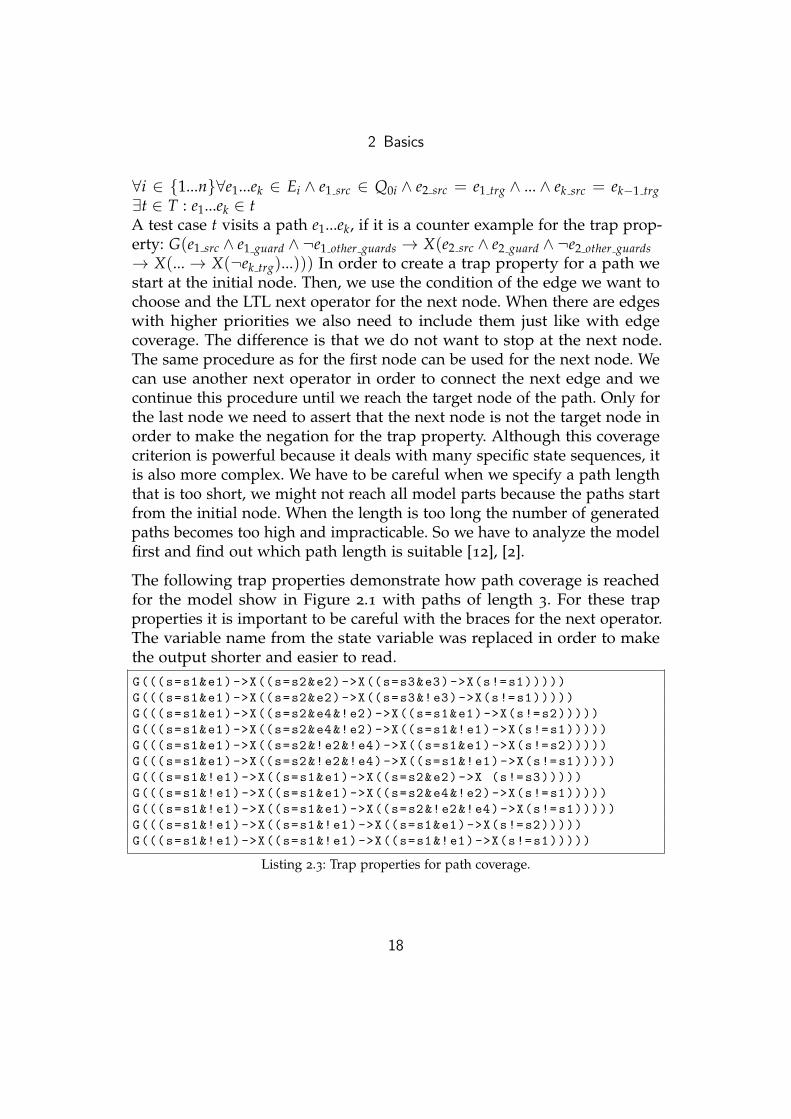
∀i ∈ {1...n}∀e1...ek ∈ Ei ∧ e1 src ∈ Q0i ∧ e2 src = e1 trg ∧ ... ∧ ek src = ek−1 trg∃t ∈ T : e1...ek ∈ tA test case t visits a path e1...ek, if it is a counter example for the trap prop-erty: G(e1 src ∧ e1 guard ∧ ¬e1 other guards → X(e2 src ∧ e2 guard ∧ ¬e2 other guards→ X(...→ X(¬ek trg)...))) In order to create a trap property for a path westart at the initial node. Then, we use the condition of the edge we want tochoose and the LTL next operator for the next node. When there are edgeswith higher priorities we also need to include them just like with edgecoverage. The difference is that we do not want to stop at the next node.The same procedure as for the first node can be used for the next node. Wecan use another next operator in order to connect the next edge and wecontinue this procedure until we reach the target node of the path. Only forthe last node we need to assert that the next node is not the target node inorder to make the negation for the trap property. Although this coveragecriterion is powerful because it deals with many specific state sequences, itis also more complex. We have to be careful when we specify a path lengththat is too short, we might not reach all model parts because the paths startfrom the initial node. When the length is too long the number of generatedpaths becomes too high and impracticable. So we have to analyze the modelfirst and find out which path length is suitable [12], [2].

The following trap properties demonstrate how path coverage is reachedfor the model show in Figure 2.1 with paths of length 3. For these trapproperties it is important to be careful with the braces for the next operator.The variable name from the state variable was replaced in order to makethe output shorter and easier to read.G(((s=s1&e1)->X((s=s2&e2)->X((s=s3&e3)->X(s!=s1)))))

G(((s=s1&e1)->X((s=s2&e2)->X((s=s3&!e3)->X(s!=s1)))))

G(((s=s1&e1)->X((s=s2&e4&!e2)->X((s=s1&e1)->X(s!=s2)))))

G(((s=s1&e1)->X((s=s2&e4&!e2)->X((s=s1&!e1)->X(s!=s1)))))

G(((s=s1&e1)->X((s=s2&!e2&!e4)->X((s=s1&e1)->X(s!=s2)))))

G(((s=s1&e1)->X((s=s2&!e2&!e4)->X((s=s1&!e1)->X(s!=s1)))))

G(((s=s1&!e1)->X((s=s1&e1)->X((s=s2&e2)->X (s!=s3)))))

G(((s=s1&!e1)->X((s=s1&e1)->X((s=s2&e4&!e2)->X(s!=s1)))))

G(((s=s1&!e1)->X((s=s1&e1)->X((s=s2&!e2&!e4)->X(s!=s1)))))

G(((s=s1&!e1)->X((s=s1&!e1)->X((s=s1&e1)->X(s!=s2)))))

G(((s=s1&!e1)->X((s=s1&!e1)->X((s=s1&!e1)->X(s!=s1)))))

Listing 2.3: Trap properties for path coverage.

18

2 Basics

2.7 Logic-based Coverage

The description in this section is based on the work from Ammann, Offutt,and Xu [2] and the formal definitions are based on the work from Bloemet al. [5]. Logic-based coverage criteria are coverage metrics that are appliedto logical expressions. In contrast to graph-based coverage criteria theydeal with predicates and clauses and not with graph components. Logicalexpressions can occur in a variety of places in software, but for this thesislogic-based coverage criteria are applied to the edge conditions or guards ofthe given formal models.

A clause is an expression that can be true, false, a Boolean variable orthe conjunction between two Boolean or non-Boolean variables with thefollowing notion: {a > b; a ≥ b; a < b; a ≤ b; a = b; a 6= b} It does notcontain any logical operators. A predicate is a logical expression and it isevaluated to true or false. It can be a clause or the conjunction of multipleclauses or predicates with the following logic operators: { ¬p; p1 ∧ p2;p1∨ p2 }. For our models the predicates are the edge conditions or guardsof the edges. For the definition of logic-based coverage, we introduce thefollowing semantics: A test case t for a predicate p is an assignments for allvariables t : V → D. For the evaluation of the truth value of a predicate por a clause c we write p(t) and c(t). A clause c is part of the set of clausesof a predicate c ∈ Cs(p).

2.7.1 Predicate Coverage

Predicate coverage is a simple form of coverage, it requires that each predi-cate has to evaluate to true and false at least one time. Predicate coverageis fulfilled by a test suite T, iff for each predicate: ∃t, t′ ∈ T : p(t) ∧ ¬p(t′).A problem of this coverage criterion is that only the predicates as a wholeare evaluated and not the clauses and so when there is a problem with aclause, this might not be covered. For example when there is a clause in themodel that is not correctly mapped in the SUT, then the test cases, whichare generated with this coverage criterion might not find this bug [2].

19

2 Basics

2.7.2 Clause Coverage (CC)

Clause coverage (CC) as referred from [2] is accomplished when each clauseof each predicate evaluates to true and false at least once. A test suite Tfulfills clause coverage, iff for each predicate: ∀c ∈ Cs(p) : ∃t, t′ ∈ T :c(t) ∧ ¬c(t′). Although this coverage criterion considers all clauses, it hasthe problem that it is not guaranteed that predicate coverage is fulfilledwhen clause coverage is fulfilled. For example when there is a predicate withsome clauses, it is possible to make two assignments, one arbitrary and one,which has each clause inverted of this arbitrary assignment. Then, these twoassignments fulfill clause coverage, but not necessarily predicate coverage.This problem can be easily shown with a simple predicate p = a > b∨ b = 5,which can have 4 possible assignments as demonstrated in Table 2.1: For

a b a >b b = 5 a > b ∨ b = 51 6 5 T T T2 3 2 T F T3 4 5 F T T4 2 6 F F F

Table 2.1: Truth table with variable assignments for the demonstration of clause coverage.

this predicate the assignments from row 2 and row 3 would be enoughto fulfill clause coverage, but these two rows would not fulfill predicatecoverage. Therefore, clause coverage does not implicate predicate coverage.However, for many cases predicate coverage is reached when test cases forclause coverage are generated. For example when row 1 and row 4 wouldbe used, then both clause coverage and predicate coverage are reached. Theproblem with this coverage criterion is that important branches from theSUT could be missed because not all condition cases are evaluated.

2.7.3 Combinatorial Coverage (CoC)

Combinatorial coverage (CoC), sometimes also called multiple conditioncoverage, requires that for each predicate all possible combination of truthvalues must be evaluated for the clauses. CoC is fulfilled by a test suite T,

20

2 Basics

iff for each predicate for all clauses c1...cn ∈ Cs(p):∃t ∈ T : c1(t) ∧ c2(t) ∧ ...∧ cn(t)∧∃t ∈ T : ¬c1(t) ∧ c2(t) ∧ ...∧ cn(t)∧∃t ∈ T : c1(t) ∧ ¬c2(t) ∧ ...∧ cn(t)∧∃t ∈ T : ¬c1(t) ∧ ¬cn(t) ∧ ...∧ cn(t) ∧ ...∧∃t ∈ T : c1(t) ∧ c2(t) ∧ ...∧ ¬cn(t)∧∃t ∈ T : ¬c1(t) ∧ c2(t) ∧ ...∧ ¬cn(t)∧∃t ∈ T : c1(t) ∧ ¬c2(t) ∧ ...∧ ¬cn(t) ∧ ...∧∃t ∈ T : ¬c1(t) ∧ ¬c2(t) ∧ ...∧ ¬cn(t).This is equivalent to taking all rows from the truth table of each predicateand forming a test case of each row. When we have a predicate with n inde-pendent clauses it produces 2n test cases. Although this coverage criterionincludes both clause and predicate coverage, the problem with this criterionis that the number of test cases becomes too large and therefore it is notpractically usable, when the number of clauses is not very small [2].

2.7.4 Active Clause Coverage (ACC)

Active clause coverage (ACC) requires that each clause is tested undercircumstances where it affects the predicate value. This is done to avoid anaffect called masking, where regardless of the value of a clause the valueof the predicate does not change. Therefore, it is required that the valueof the predicate changes, when the value of a clause is changed. In orderaccomplish such an approach, the concepts of major clause and minor clausewere introduced. In order to define these concepts formally, we introducethe following semantics: A clause c is a major clause, if it determines thevalue of p for a test case: det(c, p, t), iff p(t) 6= p[c|¬c(t)](t). This meansthat the value of the predicate is changed, when the value of the clause ischanged. The other clauses, called minor clauses c′, then must have valuesthat allow a change of the predicate value when the major clause value ischanged. In order to achieve active clause coverage it is required that foreach major clause and predicate, the minor clauses have to be chosen, sothat the major clause determines the value of the predicate and also the trueand the false case of the major clause must be evaluated [2], [5].

21

2 Basics

The advantage of this approach is that it accomplishes both predicate cover-age and clause coverage and the number of test cases that are required forthis approach is also manageable. ACC is very similar to earlier descriptionsof modified condition decision coverage (MCDC), which is a very commoncode coverage criterion. However, there were some disagreements about thedefinition, concerning what should be done with the minor clause. There-fore, different versions of ACC are mentioned: The most general version iscalled general active clause coverage (GACC), which makes no limitationsfor the minor clauses. GACC is fulfilled by a test suite T, iff for each pred-icate: ∀c ∈ Cs(p) : ∃t, t′ ∈ T : c(t) ∧ ¬c(t′) ∧ det(c, p, t) ∧ det(c, p, t′). Theproblem with this approach is that it does not imply predicate coverageand therefore other versions of ACC, which are described in the followingsections, should be preferred [2], [5].

2.7.5 Correlated Active Clause Coverage (CACC)

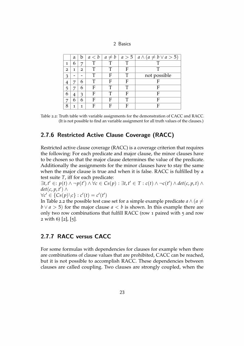
Correlated active clause coverage (CACC) is also referred to as maskingMCDC. It requires that for each predicate and each major clause, the valuesof the minor clauses must be chosen, so that the value of the major clausedetermines the value of the predicate and the both the true and the falsecase of the predicate must be evaluated. CACC is fulfilled by a test suite T,iff for each predicate:∃t, t′ ∈ T : p(t) ∧ ¬p(t′) ∧∀c ∈ Cs(p) : ∃t, t′ ∈ T : c(t) ∧ ¬c(t′) ∧ det(c, p, t) ∧ det(c, p, t′)Table 2.2 shows test cases for the major clause a for an example predicatea ∧ (a 6= b ∨ a > 5). It is apparent that the major clause a < b dictates thepredicate value when the a 6= b ∨ a > 5 part is true, which is the case fortwo assignments. Any combination of these assignments with the true andfalse case of the major clause makes a test case set that accomplishes CACC.For the given example this is done by choosing a pair of test cases one fromrow 1 and 2 and the other from row 5, 6 and 7. This results in 6 possiblecombinations that fulfill CACC for the major clause a < b [2], [5].

22

2 Basics

a b a < b a 6= b a > 5 a ∧ (a 6= b ∨ a > 5)1 6 7 T T T T2 1 2 T T F T3 - - T F T not possible4 7 6 T F F F5 7 6 F T T F6 4 3 F T F F7 6 6 F F T F8 1 1 F F F F

Table 2.2: Truth table with variable assignments for the demonstration of CACC and RACC.(It is not possible to find an variable assignment for all truth values of the clauses.)

2.7.6 Restricted Active Clause Coverage (RACC)

Restricted active clause coverage (RACC) is a coverage criterion that requiresthe following: For each predicate and major clause, the minor clauses haveto be chosen so that the major clause determines the value of the predicate.Additionally the assignments for the minor clauses have to stay the samewhen the major clause is true and when it is false. RACC is fulfilled by atest suite T, iff for each predicate:∃t, t′ ∈: p(t) ∧ ¬p(t′) ∧ ∀c ∈ Cs(p) : ∃t, t′ ∈ T : c(t) ∧ ¬c(t′) ∧ det(c, p, t) ∧det(c, p, t′) ∧∀c′ ∈ {Cs(p)\c} : c′(t) = c′(t′)In Table 2.2 the possible test case set for a simple example predicate a∧ (a 6=b ∨ a > 5) for the major clause a < b is shown. In this example there areonly two row combinations that fulfill RACC (row 1 paired with 5 and row2 with 6) [2], [5].

2.7.7 RACC versus CACC

For some formulas with dependencies for clauses for example when thereare combinations of clause values that are prohibited, CACC can be reached,but it is not possible to accomplish RACC. These dependencies betweenclauses are called coupling. Two clauses are strongly coupled, when the

23

2 Basics

change of the value of one clause always changes the value of the other.They are weakly coupled, when the change of the value of one clause onlysometimes affects the other clause [8]. The problem with RACC is that itdoes not allow a very flexible assignment of combinations. As it was shownin the previous simple example for RACC there were only two possibleways to make a test case set. For CACC there were six possible ways andthe assignment of the minor clauses could also be selected more flexible,which makes the generation of test cases for CACC easier [2].

24

3 Related work

The first approach in the area of model-based testing respectively testingbased on formal specifications, was presented by Bernot, Gaudel, and Marre[3]. Many other publications followed after this work: [33], [23], [22], [12].

However, many approaches only focus on a theoretical definition of cov-erage criteria and have no practical implementation or evaluations on realworld examples. For instance Fraser, Wotawa, and Ammann [12] presenteda survey of different testing methods with model checkers and showedadvantages and issues. Furthermore, they gave an overview of coveragecriteria, trap property definition and mutation-based test case generation.Weyuker, Goradia, and Singh [33] also showed a more theoretical approachto generate test data from specifications. Weißleder [32] gave a broadertheoretical overview of model-based testing and also showed a method forcombining coverage criteria, but another combination approach and alsodifferent model types were used.

Some approaches have a stronger focus on test case generation for the dataflow in the program and not control flow. For example, Hong et al. [17]showed an approach in the area of data flow testing, where an extendedversion of temporal logic and definition-use pairs for variables were used inorder to describe certain data flow coverage criteria.

Fraser [11] gave an overview of test case generation with model check-ers. The focus of this work was more towards optimization possibilitiesfor test case generation. So evaluations about the effectiveness of testing,improvement of LTL formulas, model checker performance and mutantminimization and many other optimization aspects, were shown.

Some approaches focus more on logic-based coverage criteria, for exampleBloem et al. [5] showed an evaluation of CACC or MCDC and it was also

25

3 Related work

analyzed how this coverage criterion could be applied to a real practicalsystem. Furthermore, the developed CACC tool was compared with hand-crafted tests and it was shown how much code coverage could be reached.Chilenski [8] also showed a comparison of different coverage criteria, butthe focus was also only on logic-based coverage criteria.

Lahtinen [20] gives a good overview of temporal logic and about NuSMV.This work also showed how NuSMV counter examples are created and howthey can be converted in a different simplified representation.

A very similar work was presented by Offutt et al. [22], which showed atest data generation technique from formal specifications with MCDC. Theypresented an approach, where parse trees for decisions are traversed inorder to generate test cases for MCDC. They also evaluated this approachwith small examples and with a case study. However, the difference is thatthis approach has more limitations, it only works for Boolean variables.Another difference is that the work did not show different approaches for acombination of logic-based and graph-based coverage criteria.

The closest related work we found was from Ammann, Offutt, and Xu[2]. It was also focused on coverage criteria. Many different versions ofgraph-based and logic-based coverage criteria are explained and comparedin this work. Furthermore, it was shown how logic based coverage criteriacan be applied for formal models in the form of state machines. The authorsdemonstrated this approach on a small example. However, the difference isthat they did not show an extensive evaluation of their approach with realworld examples and they did not demonstrate a practical implementationof their approach. Furthermore, they did not show how logic-based andgraph-based coverage criteria could be combined in different ways.

There are other similar tools that can be used to generate test cases as well.For example, Spec Explorer also is a tool for model-based testing. However,it uses a symbolic exploration algorithm on the model in order to generatetest cases [31]. Our tool uses trap properties and a model checker for the testcase generation. Another example is Uppaal Cover [16]. This test generationtool also supports automatic test case generation for a dynamically selectedcoverage criterion. For example it offers node or edge coverage, but itdoes not provide logic-based coverage criteria and it also uses a differentgeneration method.

26

4 Combination Method forCoverage Criteria

In this chapter we describe our combination methods for graph-based andlogic-based coverage criteria. We combine edge coverage and path coveragewith CACC. Node coverage was not combined with CACC, because it doesnot deal with edge conditions and CACC only is applied to them. The ideaof the combinations is to increase the coverage of the generated test caseson the model and the SUT by applying the strengths of both logic-basedand graph-based coverage criteria. With our combination methods we wantto create test cases that reach a better coverage than a method that only usesgraph-based or logic-based coverage. In addition, our combination methodsshould be practically usable and produce a manageable number of test casesfor real world projects.

4.1 Combination of Edge Coverage with CACC

Our combination of edge coverage with CACC is fulfilled for a modelM = M1 × ...× Mn by test suite T = {{q0a0q1a1...}, {q0a0q1a1...}, ...} andq0a0q1a1... is a sequence of states q0, q1, ... ∈ Qi and assignments sets a, iff:∀i ∈ {1...n}∀e ∈ Ei, if p = eguard ∧ ¬eother guards∃qjajqk ∈ T : qj = esrc ∧ p(aj) ∧ qk = etrg∧∃a, a′ ∈ T : p(a) ∧ ¬p(a′) ∧∀c ∈ Cs(p) : ∃a, a′ ∈ T : c(a) ∧ ¬c(a′) ∧ det(c, p, a) ∧ det(c, p, a′)

For the creation of the combined trap properties we use the trap propertiesfor edge coverage as explained in Section 2.6.2. From each of these trapproperties we use the guard and the negation of the guards of the other

27

4 Combination Method for Coverage Criteria

edges with higher priority eguard ∧¬eother guards as input formula to generatethe assignments for CACC. For the generation we used an external tool thatwas presented by Bloem et al. [5]. This CACC tool uses an SMT solver toproduce the variable assignments and it can handle complex input formulasvery fast.

CACC produces sets of assignments for the included variables in the inputformula. These assignment sets A can be used as predicates as well andwe combine them with the original trap property by replacing the inputformula. The original trap property has the following form:

G(esrc ∧ eguard ∧ ¬eother guards → X(¬etrg))

For each assignment set we create a separate new trap property as follows:

∀a ∈ A :

{G((esrc ∧ a)→ X(¬etrg)) if a makes eguard ∧ ¬eother guards true

G((esrc ∧ a)→ X(etrg)) if a makes eguard ∧ ¬eother guards false

CACC includes both true and false cases for the input formula. In orderto create trap properties that negate a property, we have to handle the trueand false cases differently. For the true cases, we can keep the negation forthe target state of the original trap property. For a false case we remove thenegation because when the guard is false or when the guard of a higherpriority edge is true, then a different edge will be used and a different targetstate will be reached. Therefore, the trap property states that the next stateis the target state of the edge. This is not true for an assignment set for afalse case and so we have the necessary negation for the trap property.

4.2 Combination of Path Coverage with CACC

Path coverage with CACC for all path of length k is fulfilled for a modelM = M1 × ...× Mn by test suite T = {{q0a0q1a1...}, {q0a0q1a1...}, ...}, iff:∀i ∈ {1...n}∀e1...ek ∈ Ei ∧ e1 src ∈ Q0i ∧ e2 src = e1 trg ∧ ...∧ ek src = ek−1 trg, ifp = ek guard ∧ ¬ek other guards∃q0a0...ak−1qk ∈ T : q0 = e1 src ∧ e1 guard(a0) ∧ ...∧ p(ak−1) ∧ qk = ek trg∧∃a, a′ ∈ T : p(a) ∧ ¬p(a′) ∧∀c ∈ Cs(p) : ∃a, a′ ∈ T : c(a) ∧ ¬c(a′) ∧ det(c, p, a) ∧ det(c, p, a′)

28

4 Combination Method for Coverage Criteria

The combination of path coverage with CACC was done similar to edgecoverage, but the variable assignment sets generated by the external CACCtool were only applied to the last edge of the path. For path coverage asdescribed in Section 2.6.3 we have trap properties in the following form:G(e1 src ∧ e1 guard ∧ ¬e1 other guards → X(e2 src ∧ e2 guard ∧ ¬e2 other guards→ X(...→ X(ek src ∧ ek guard ∧ ¬ek other guards → X(¬ek trg))...)))

For our combination approach we apply CACC for the last edge ek ofeach path e1...ek. As input formula for CACC we use ek guard ∧¬ek other guards,just as for edge coverage with CACC and also sets of assignments A areproduced for the included variables. For each assignment set a ∈ A wecreate a separate new trap property as follows:if a makes ek guard ∧ ¬ek other guards true:G(e1 src ∧ e1 guard ∧ ¬e1 other guards → X(e2 src ∧ e2 guard ∧ ¬e2 other guards→ X(...→ X(ek src ∧ a→ X(¬ek trg))...)))if a makes ek guard ∧ ¬ek other guards false:G(e1 src ∧ e1 guard ∧ ¬e1 other guards → X(e2 src ∧ e2 guard ∧ ¬e2 other guards→ X(...→ X(ek src ∧ a→ X(ek trg))...)))

We apply CACC only to the last edge because otherwise the number oftrap properties would be unmanageable, when all CACC assignments ofone edge would be combined with the CACC assignments of other edges.The problem with this approach is that CACC might not be applied forthe first edges in the path. However, it is possible to use the path coveragealgorithm for all paths up to a certain length. With this method CACC canalso be applied for the first edges in a path, without creating too many trapproperties.

29

5 Tool Development

In order to show that the described coverage criteria present a compellingmethod to create abstract test cases and also to show that they are prac-tically usable, we developed a Java Tool. This tool uses a given NuSMVmodel file as input and generates test cases as output, which fulfill a certainselected coverage criterion. These test cases can be used by a test adapter inorder to test the functionality of a SUT. Java was used for the developmentbecause it is platform independent and also because there were alreadyexisting projects, which are described later. We designed our tool with acomponent-based structure in order to make it easily extendable and toallow the integration of further coverage criteria. Furthermore, we includeda feature for process handling in order to make it possible to use external ap-plications, for example for model checking or for the assignment generationfor CACC.

In this chapter the development process of the tool, the component structure,included external applications, algorithmic design and configuration optionsare explained. Furthermore, additional features like model visualizationand known limitations of the tool are mentioned.

5.1 Component Structure

We developed the tool with object-oriented programming and separated itin different components for the different tasks of the generation process.The first component is the model parser, which takes the given NuSMV fileand makes an object representation, which has class instances for the modelcomponents. The model contains at least one deterministic variable, whichis represented as a graph. The states are represented as node objects and

30

5 Tool Development

the transitions as edge objects. The representation is then used by the testcase generator component, which uses it to traverse over the graphs andcreates trap properties according to a certain selected coverage criterion.

Instead of including edge conditions in the trap properties, it is also possibleto include variable assignments. These assignments are generated by anexternal tool that takes the edge condition as input and produces test datafor CACC. We write the formulas from the edge conditions in an input file.Then a process is started for the CACC tool, which reads the input file andproduces assignment for the variables that are part of these conditions. Theseassignments are then used for the trap property definition. The developmentand analysis of the CACC tool was described in [5].

After all trap properties are created, a NuSMV process is started, which usesthem and the NuSMV model file in order to create counter example traces.These traces represent abstract test cases and a test adapter can executethem on the SUT.

Figure 1.1 shows an overview of the tool components and the inputs andoutputs of each component are displayed. Furthermore, the correlationrespectively the sequence, in which the components are used, is shownand also where the configuration arguments from the user are applied andwhere the given external tool is used.

5.2 Model Parsing

The first important part of the tool is the model parser. This component usesa given NuSMV file as input and generates an object structure. The modelparts that are relevant for this object structure are the variable definitions andstate transitions and initial states for deterministic variables. The variabledefinitions include the name of the variable, the type and the options forenumeration type variables. The state transitions include the source and thetarget state and also a condition that has to be fulfilled so that the transitioncan occur. In order to extract information from the given NuSMV modelfile and convert it in a form that is processable, it was necessary to find asuitable parsing solution.

31

5 Tool Development

Due to the fact that model or file parsing is a common task, this part wasnot implemented from scratch. A few projects were analyzed in order tofind a usable solution, which already performs parsing of NuSMV files. AnXtext project called NuSMV-Tools [14] was found, which accomplished thistask properly.

5.2.1 Xtext

Xtext is an open source framework for the development of programminglanguages and domain specific languages and it is mostly used in combi-nation with the Eclipse integrated development environment (IDE) [24]. Itprovides the possibility to develop language extensions for Eclipse and easyways to accomplish features like syntax tree generation, syntax highlighting,editor tools, parsing and so on. For this project only the parsing processwas relevant.

5.2.2 Conversion of the Parsed Object Structure

After the NuSMV file is parsed with the given parser, the produced objectstructure needs some conversions. This is necessary because it includesunnecessary information and complicated representation forms. Some parts,for which a string representation is enough, are stored in a complicatedabstract form. In order to produce a usable object structure, many partsare stored in different classes. For nodes, edges and variables separatedclasses are used with associated attributes. Nevertheless, for some modelparts the generated structure is already very convenient. For instance theedge conditions or guards are already stored in a recursive tree structure,which makes it easy to process these formulas.

5.2.3 Parsed Model Structure

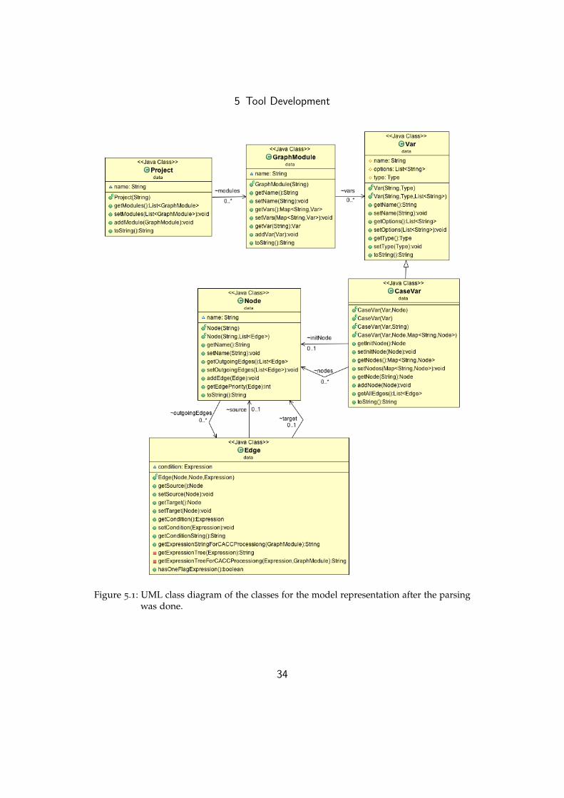
In Figure 5.1 the UML class diagram of the model classes is shown. Theseclasses are for the object structure of the parsed model. The attributes of

32

5 Tool Development

a model are mapped in a project object, which consists of one or moremodules. Each of these modules can have a number of variables and theyare divided in two groups. There are deterministic and nondeterministicvariables, which are represented with the same base class. The differenceis that the deterministic variables include a graph representation and haveclasses for nodes and edges.

5.3 Model Visualization

Visualization is a useful feature, in order to verify manually that the parsingwas done correctly and that the model was designed as expected. It alsohelps to provide a quick general view of the model and this makes it possibleto check easily, if there are any flaws. For example, it can be used to check,if there are no missing edges or if an edge is misplaced between the wrongnodes.

To visualize the object structure, each object has a toString method and thecombined output of these methods is a DOT string. DOT from Graphviz[10] is a textual description language for graphs. It offers a very simple wayto describe a graph in a textual form and there are various tools that are ableto generate a visual image of the graph from this textual representation. Thegreat advantage of the DOT description language is that it is not requiredto deal with aspects like the positioning of the nodes or how the edges areplaced. These settings are automatically chosen from the generation toolsand most of the time the generated graph is formatted neatly. However,there are many styling options that are useful to change some default designdecisions or to change the formatting or styling features [19], [13].

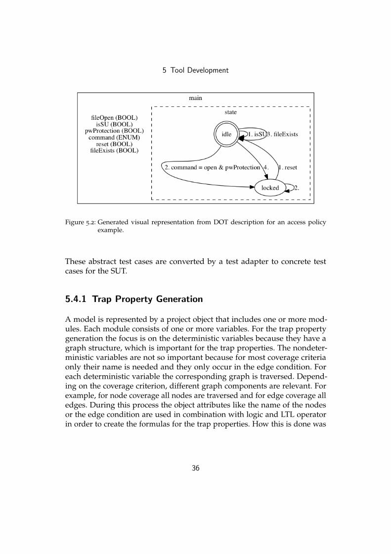
Listing 5.1 shows the generate DOT description of the model of an accesspolicy system and in Figure 5.2 the generated visual image, representationfrom the described graph, is shown. The model of this example demonstratesa simple conceptual access policy system, which regulates the access to thefile system. In this example the access to the file system should only begranted to users with the required permissions. For example a user, whichhas super user permissions should be allowed to access the file system.Furthermore, it should not be allowed to open files that are password

33

5 Tool Development

Figure 5.1: UML class diagram of the classes for the model representation after the parsingwas done.

34

5 Tool Development

protected. When one of the access rules is violated, the system goes in thelocked state, otherwise it remains in the idle state.

digraph AccessPol{ subgraph clustermain {l a b e l =”main ” ;vars [ shape = none l a b e l =” f i leOpen (BOOL) \n

isSU (BOOL) \npwProtection (BOOL) \ncommand(ENUM) \nr e s e t (BOOL) \nf i l e E x i s t s (BOOL) \n ” ] ;

subgraph c l u s t e r s t a t e { s t y l e = ”dashed ” ;l a b e l = ” s t a t e ” ;

i d l e [ shape= d o u b l e c i r c l e ] ;locked ;locked −> i d l e [ l a b e l =”1 . r e s e t ” ] ;i d l e −> i d l e [ l a b e l =”1 . isSU ” ] ;i d l e −> locked [ l a b e l =” 2 . command = open & pwProtection ” ] ;i d l e −> locked [ l a b e l =”4 . ” ] ;i d l e −> i d l e [ l a b e l =”3 . f i l e E x i s t s ” ] ;locked −> locked [ l a b e l =”2 . ” ] ; }

}}

Listing 5.1: DOT output of a small access policy example.

5.4 Test Case Generation

For the test case generation we used the object structure, which was cre-ated by the model parser. According to a user selected coverage criterion,the graphs from the object structure are traversed in order to create trapproperties. These trap properties are given to a symbolic model checker,which checks if the given formulas are true or false for the model. For avalid trap property the formula must be false and then the model checkerproduces a counter example, which can be used as an abstract test case.

35

5 Tool Development

Figure 5.2: Generated visual representation from DOT description for an access policyexample.

These abstract test cases are converted by a test adapter to concrete testcases for the SUT.

5.4.1 Trap Property Generation

A model is represented by a project object that includes one or more mod-ules. Each module consists of one or more variables. For the trap propertygeneration the focus is on the deterministic variables because they have agraph structure, which is important for the trap properties. The nondeter-ministic variables are not so important because for most coverage criteriaonly their name is needed and they only occur in the edge condition. Foreach deterministic variable the corresponding graph is traversed. Depend-ing on the coverage criterion, different graph components are relevant. Forexample, for node coverage all nodes are traversed and for edge coverage alledges. During this process the object attributes like the name of the nodesor the edge condition are used in combination with logic and LTL operatorin order to create the formulas for the trap properties. How this is done was

36

5 Tool Development

already described in Section 2.6 and further implementation details willfollow in Section 5.5.

5.4.2 Counter Example Generation

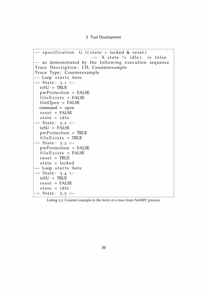
The generated trap properties from the test generator component are usedas input for a symbolic model checker. In this implementation NuSMV wasnot only used in order to specify the model, but also as symbolic modelchecker. So a NuSMV process is started, then the model is loaded and theformulas for the trap properties are given to the process one by one. If a trapproperty is valid the symbolic model checker returns a counter example inthe form of an execution trace, otherwise it states that the formula is true forthe given model and no counter example is generated. Each of these counterexamples is then written to the output file for the test cases. After the testcase generation process is finished, a test adapter can use this output file.So a test adapter can parse the abstract test cases from the file and thenexecute them as concrete test cases on the SUT. Due to the fact that eachSUT needs an individual test adapter, we described it for each illustratedSUT separately.

Listing 5.2 shows a counter example for a trap property for edge coverage,applied to the model shown in Figure 5.2. It can be seen that the NuSMVprocess states that the formula from the trap property is false. Furthermore, aLTL Counterexample in the form of a trace is shown. This trace demonstrateshow a change of the nondeterministic variables influences the deterministicvariables.

37

5 Tool Development

−− s p e c i f i c a t i o n G ( ( s t a t e = locked & r e s e t )−> X s t a t e != i d l e ) i s f a l s e

−− as demonstrated by the fol lowing execut ion sequenceTrace Descr ipt ion : LTL CounterexampleTrace Type : Counterexample−− Loop s t a r t s here−> S t a t e : 5 . 1 <−

isSU = TRUEpwProtection = FALSEf i l e E x i s t s = FALSEfi leOpen = FALSEcommand = openr e s e t = FALSEs t a t e = i d l e

−> S t a t e : 5 . 2 <−isSU = FALSEpwProtection = TRUEf i l e E x i s t s = TRUE

−> S t a t e : 5 . 3 <−pwProtection = FALSEf i l e E x i s t s = FALSEr e s e t = TRUEs t a t e = locked

−− Loop s t a r t s here−> S t a t e : 5 . 4 <−

isSU = TRUEr e s e t = FALSEs t a t e = i d l e

−> S t a t e : 5 . 5 <−Listing 5.2: Counter example in the form of a trace from NuSMV process.

38

5 Tool Development

5.5 Implemented Coverage Criteria

In this section we describe the actual coverage criteria, which are supportedfrom our tool, and we highlight how they were implemented. First, we illus-trate the graph-based coverage criteria and then our combination approachfor logic-based and graph-based coverage criteria.

5.5.1 Graph-based Coverage Criteria

The implementation of graph-based coverage criteria was done accordingto the definitions in Section 2.6 and by using the data from the parsedmodel. For node coverage it was required to iterate over all node objects.During this iteration the name of the node and the concerning variablename was used in order to create the formulas for the trap properties. Theimplementation of edge coverage required an iteration loop over all edgeobjects. For each edge the guard or edge condition, the name of the targetnode and the source node were used for the trap property formulas. Foredges that did not have the highest priority, it was also important to includethe negated guards of the higher priority edges in the formula. Therefore,the guards of the previous iteration steps were stored so that they could beused later in negated form for the formulas for lower priority edges. Detailsfor the creation of the formulas can be found in Section 2.6.

The implementation of trap properties for path coverage was more complexthan for node or edge coverage, because an algorithm with iteration was notenough to build the requested paths. Therefore, a recursive algorithm wasdesigned, which goes to each outgoing edge of a node and continues to callitself again for the target nodes of the outgoing edges. During this process,the data that is needed for the trap properties is obtained from the nodesand edges and the process stops when the path has reached the length thatwas specified from the input parameter.

When the user specifies that all paths up to a certain length are needed,then this algorithm for path coverage is simply executed several times forthe different lengths.

39

5 Tool Development

5.5.2 Combination of Graph-based Coverage with CACC

As explained in Section 5.1, an external tool [5] for the generations ofvariable assignments for CACC coverage was used. In order to integratethis tool, it was started as a separate process. We used the Java processbuilder, which provides an easy way to manage a process and to interactwith this process. In order to communicate with the process of the CACCtool, we write the formula for the edge conditions in an input file. (This isdone for each edge separately.) Then, the process runs and uses the formulafrom this input file to generate an output file with a number of assignmentsets for the variables that occur in the edge conditions. Each of these setshas assignment values for a separate test case and it contains values forall variables that were included in the input formula. The assignment setsare used in combination with the trap property of the associated edge. Thecombination was done as described in Section 4.1.

The assignment sets have one limitation. It is not clear if a given assignmentset represents a true or false case for the edge condition. CACC includesboth true and false cases for the input formula and the output of the CACCtool provides no way to distinguish them. Hence, we create a second trapproperty for each CACC assignment set, which has no negation of theexpected next state. This is done because for a false case the next state isnot the expected target state from the edge, but could be any target statethat is reachable with an outgoing edge. Therefore, the trap property statesthat the next state is the target state from the edge. This is not true for anassignment set for a negative case and so we have the necessary negationfor the trap property.

Listing 5.3 shows the generated CACC assignment sets for the followingedge condition:

! doClose & doOpen & lock != locked

This edge condition is from the door variable of the car alarm example,which is explained in Section 6.2 and illustrated in Figure 6.5. In order tofulfill the requirements for the CACC tool, the formula needs conversions,which are demonstrated in the following example:

( ˜ ( doClose ) ) & ( doOpen ) & (lock CONV ENUM != 1 )

40

5 Tool Development

It can be seen that the enumerative type variable in this condition is markedwith a placeholder ” CONV ENUM” and that the value is replaced withan integer. This is done, because the CACC tool does not directly supportenumerative type variables. The assignment sets that are generated forthis input formula are shown in Listing 5.3. After the assignment sets aregenerated, the replacements for the enumerative type variable is convertedback, so that it can be used for the trap properties. The trap properties thatwere generated for the assignment sets are shown in Listing 5.4.

The combination of path coverage with CACC as described in Section 4.2was done similar to edge coverage. The only difference is that the variableassignment sets generated by the external CACC tool were only applied tothe last edge of the path. The implementation for edge coverage with CACCcould be reused and no major changes were necessary.

>> Test Nr . 1 : ( makes the input formula f a l s e )doClose = 1

doOpen = 1

lock CONV ENUM = 0

>> Test Nr . 2 : ( makes the input formula true )doClose = 0

doOpen = 1

lock CONV ENUM = 0

>> Test Nr . 3 : ( makes the input formula f a l s e )doClose = 0

doOpen = 0

lock CONV ENUM = 2

>> Test Nr . 4 : ( makes the input formula f a l s e )doClose = 0

doOpen = 1

lock CONV ENUM = 1

Listing 5.3: Generated test case assignments from the CACC tool.

41

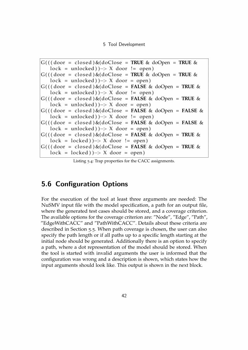
5 Tool Development

G( ( ( door = closed ) &(doClose = TRUE & doOpen = TRUE &lock = unlocked ) )−> X door != open )

G( ( ( door = closed ) &(doClose = TRUE & doOpen = TRUE &lock = unlocked ) )−> X door = open )

G( ( ( door = closed ) &(doClose = FALSE & doOpen = TRUE &lock = unlocked ) )−> X door != open )

G( ( ( door = closed ) &(doClose = FALSE & doOpen = TRUE &lock = unlocked ) )−> X door = open )

G( ( ( door = closed ) &(doClose = FALSE & doOpen = FALSE &lock = unlocked ) )−> X door != open )

G( ( ( door = closed ) &(doClose = FALSE & doOpen = FALSE &lock = unlocked ) )−> X door = open )

G( ( ( door = closed ) &(doClose = FALSE & doOpen = TRUE &lock = locked ) )−> X door != open )

G( ( ( door = closed ) &(doClose = FALSE & doOpen = TRUE &lock = locked ) )−> X door = open )

Listing 5.4: Trap properties for the CACC assignments.

5.6 Configuration Options

For the execution of the tool at least three arguments are needed: TheNuSMV input file with the model specification, a path for an output file,where the generated test cases should be stored, and a coverage criterion.The available options for the coverage criterion are: ”Node”, ”Edge”, ”Path”,”EdgeWithCACC” and ”PathWithCACC”. Details about these criteria aredescribed in Section 5.5. When path coverage is chosen, the user can alsospecify the path length or if all paths up to a specific length starting at theinitial node should be generated. Additionally there is an option to specifya path, where a dot representation of the model should be stored. Whenthe tool is started with invalid arguments the user is informed that theconfiguration was wrong and a description is shown, which states how theinput arguments should look like. This output is shown in the next block.

42

5 Tool Development

Options:

-i, --input path to the NuSMV file with the model

-o, --output path to the output file, where the generated test cases

should get stored

-c, --coverage test case generation method or coverage

options: [Node, Edge, Path, EdgeWithCACC, PathWithCACC]

-p, --path-conf path length or "upto" plus length (eg. upto3)

-d, --dot-file path to the file, where the dot representation

should get stored

5.7 Additional Features

During the development and test of the tool we discovered that someNuSMV notations and some models required adjustments for the tool. Inthis section these issues are described and it is shown how it was possibleto handle them.

Define Symbol Parsing

In NuSMV the define part can be used to create symbols that work likemacros. These symbols are defined without the need for a new variable,so that the state space is not enhanced, and the computation complexitydoes not increase substantially. During execution these symbols are simplysubstituted by their assignment [7], [6].

First, we thought that the define part could be ignored during the parsingprocess, because it is not necessary for the trap property generation andis only relevant when the model checker checks the trap properties onthe model. However, we discovered that the type of these symbols wasrelevant in order to process the generated assignments of the used CACCtool. When the CACC tool produces an assignment for a variable or asymbol, the type must be known, because the used model checker does notallow assignments for integers and Boolean variables in the same way. Forexample a one must be replaced with true for a Boolean symbol in order to

43

5 Tool Development

create a valid assignment that the model checker accepts. The problem withdefined symbols is that they have no predefined types, but the type can bedetermined by inspecting the assignments. Hence, it was necessary that thedefine part of the model was also considered during the parsing process.This could be done similar to the variable parsing. The difference was thatthe type was not known at the beginning and so the assigned values wereanalyzed in order to determine the type and also to obtain the possibleoptions for enumeration type symbols.

Output and Performance Optimization

The size of some models also caused some problems. When there are manyedges, then the computation of path and edge coverage takes much moretime, because the model checker needs a lot of time to compute all counterexamples. The initial implementation did not include a progress notification,so it was not possible to see if the tool still worked properly. Hence, anoutput message was added that tells the user, how many trap propertiesare already processed, and how many are still left.

Another issue was the memory usage. First, the generated counter examplesfrom the model checker were simply stored in a list, which was placedin the memory. For small models this was not a problem because mostlythere were less than hundred counter examples. However, larger modelscould produce some thousand trap properties even for simple coveragecriteria like edge coverage with CACC. Therefore, the storage of all thecounter example traces in memory was not reasonable anymore. Thus, amodification was made so that the generated counter example traces aredirectly stored in the output file, after they are generated, so that there is noneed to buffer them all in memory and save them all at once.

Multiple Initial Nodes

Initially we only considered deterministic variables with one initial state butNuSMV supports models that can have deterministic variables that havemultiple initial states, so that the initial value is selected non-deterministically.

44

5 Tool Development

These non-deterministically selected values can only be used as inputs bya test adapter and not as expected outputs because a comparison with thereal output of the SUT is not possible [7].

The following example shows a variable initialization with multiple initialstates.

i n i t ( CacheIdx ) := {0 , 1 , 2 , 3} ;

So the parsing process needed modifications in order to support these casesand also the representation objects for the models needed adjustments. Thus,the variable definition was changed so that a list, which supports one ormore initial values respectively nodes, was used. The trap property genera-tion only needed adjustments for path coverage because the other criteriadon’t use the initial nodes, but paths start at initial nodes. Therefore, thegeneration was changed in order to generate path coverage trap propertiesfor each of these initial nodes. However, this change increases the numberof possible paths and so this coverage criterion is less practical for the givenmodel or for other models with many initial nodes.

Multiple Target Nodes

NuSMV models can have multiple target states for a single transition case.So the next state can be any of the states of the set of target states, andthe decision is made non-deterministically. A test adapter can use thesenon-deterministically selected states only as inputs for the SUT and not asexpected outputs because a comparison with the real output of the SUT isnot possible. An example of this feature and how it is used in a model isshown here:

next ( CacheIdx ) := case. . .s t a t e = i d l e & . . . : {−1 ,2 ,3} ;. . .esac ;

The changes for the parsing process and the object representation structurewere similar to the modifications that were necessary for the support of

45

5 Tool Development

multiple initial nodes. So a single reference to a target was replaced with alist of targets and the modification to the parsing process was also similar.The trap property generation needed more changes. For edge coverage andfor path coverage it was necessary to not only consider one possible targetnode for each edge, but to iterate over the list of targets and generate trapproperties for each individually. So when an edge has multiple target nodesthe trap property generation works like when there would be multipleedges, with the same source node, guard and priority, but with a differenttarget.

Target Variables

Instead of multiple target nodes, NuSMV also supports variables as targetstate. In this case the next state is determined by the value of the targetvariable and any value that can be assigned to the variable is the possiblenext value respectively state. The following example shows this feature andhow it is used in a model:

next ( cache0 ) := case. . .s t a t e =accessCacheBlock&CacheIdx =0 : cache1 ;. . .esac ;

The changes that were necessary in order to support this feature, wheresimilar to the changes for the support for multiple target nodes, but withthe difference that the trap property generation was more complex. Sothe Y-operator was used in order to check what the variable value of theprevious state was and then it is assumed that this value does not matchthe value of the associated value. This assumption is made for all possiblevariable values, as shown in the following example:

. . . −> X ! ( ( cache0 = Mx & Y( cache1 ) = Mx) |( cache0 = Dx & Y( cache1 ) = Dx) . . .

46

5 Tool Development

5.8 Known Limitations

NuSMV models can have rather complex features, which can be seen inthe manual [6]. For most models these features are not needed. Therefore,we did not implement all of them. For example case distinctions withintegers are not fully supported, because there could be rather complexcase distinctions with mathematical operations and it would be difficult tohandle them.

Another unsupported feature is case differentiations that contain multiplesource states in one formula. For example when the formula for one casecontains a disjunction of multiple source states, it is difficult to extract all ofthem and create edges for each associated node. Nevertheless, this featureis not important, because the same functionality can also be achieved whensuch a complex case formula is written in multiple parts.

Due to the fact that the CACC generation tool only supports Booleanoperators and basic arithmetic comparisons, not all mathematical operationsare supported. The tool was extended for simple cases like plus and minusof two variables, because these operations were important for an example.Most other complex mathematical operations are also not implementedfrom this tool, but they work for all other coverage criteria, where the toolis not used.

Another limitation is the computation effort. When the number of nodes oredges is to high, then the resulting number of trap properties can becomeunmanageable because the model checker would need too long to computethem all.

5.9 Define Restriction

The trap property generation process only considers certain model parts. Sowhen there are restrictions from other parts, this can cause a higher numberof invalid trap properties. For example the define part can cause restrictionsfor certain variable assignments or make some transitions impossible. Adefine restriction occurs, when there is a symbol in the define part that is

47

5 Tool Development

dependent on the values of one or more variables and therefore the symbolcan only have certain values depending on the values of these variables. Italso can occur, when there are multiple symbols with dependencies. Forexample in the case study we found a define restriction that prevented somesymbols from having the same value because they were dependent on thesame variable. These define restrictions are not a big problem for simplegraph-based coverage criteria, because they do not use specific variable orsymbol assignment for the edge conditions. However, they are an issue forthe CACC assignment generation. When certain assignment combinationsare not applicable for the model, but the input formulas for the CACCgeneration do not include these limitations, then many generated assign-ments are not usable. A solution for this problem is to identify the modelcomponents that have problems with the CACC assignment generation anduse other coverage criteria without CACC for them.

48

6 Tool Evaluation

In this chapter simple examples are shown that were used to evaluate thedeveloped tool. Different coverage criteria are compared, the functionality ofthe tool is tested and it is shown how the tool works. These simple examplemodels are functional equal to the SUTs. An abstraction was not needed,because the behavior of the SUT could be modeled nearly completely. Theonly difference is that the SUTs include input and error handling.

For each example there is a general description and a visual representation.Furthermore, an illustration of a program run can be seen and the resultsare evaluated. It is shown how the generated counter example in the formof traces are parsed and then used by a test adapter to run them on the SUT.Therefore, real implementations were made in order to show, how the inter-action with the test adapter and these implemented systems works. Theyalso were used to compare the coverage criteria on the basis of instructionand branch coverage.

6.1 Triangle Example

In this section a simple triangle example is shown that was illustrated byAichernig [1]. This example takes three numbers, which represent sidelengths of a triangle, and calculates if it is an equilateral, an isoscelesor a scalene. The example is particularly interesting, because it has edgeconditions or guards that have multiple parts with dependent variables. Soit is good to evaluate logic-based coverage because the edge conditions arenot too simple.

49

6 Tool Evaluation

6.1.1 Functional Description

The Example works as follows, first three numbers are given as input. Eachof these numbers represents the length of a triangle side. Then, according tothese lengths it is calculated, if a valid triangle can be formed. When it ispossible, the output is the kind of triangle (equilateral, isosceles, scalene)that is formed with the given lengths.

In Listing 6.2 the NuSMV model for this triangle example is shown. Theinput lengths are modeled as nondeterministic integer variables (a, b, c)that only have a limited range from 0 to 100. This range was used becauseit was enough for all interesting tests for the SUT, otherwise if it was toobig, the model checker needed too much time for the computation. Whenthe limit was bigger only the execution time of the model checker increased,but the test cases remained the same. For the representation of the output, adeterministic enumeration type variable was used, which indicates the typeof the triangle. When the lengths of two sides are smaller or equal to thelength of the third side, then it is not possible to form a triangle. Then, theoutput variable has the value ”notriangle”, which indicates that no trianglecould be formed.

6.1.2 SUT

The implementation of the SUT was quite straightforward. Basically thethree side lengths of the triangle were given as input parameters and thenthere is a case distinction in order to determine which type of triangle isformed, or if it is not possible to form a valid triangle. The result of thisdistinction is printed as output. Listing 6.1 shows the Java implementationof the SUT. It can be seen that this implementation is straightforward andshort. It only consists of input handling and of a case distinction for theoutput determination.

50

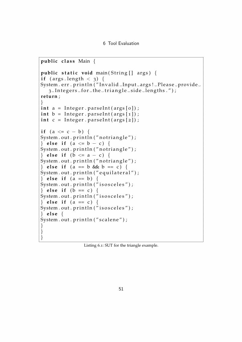
6 Tool Evaluation

public c l a s s Main {

public s t a t i c void main ( S t r i n g [ ] args ) {i f ( args . length < 3 ) {System . e r r . p r i n t l n ( ” I n v a l i d Input args ! P lease provide

3 I n t e g e r s f o r the t r i a n g l e s ide lengths . ” ) ;return ;}i n t a = I n t e g e r . p a r s e I n t ( args [ 0 ] ) ;i n t b = I n t e g e r . p a r s e I n t ( args [ 1 ] ) ;i n t c = I n t e g e r . p a r s e I n t ( args [ 2 ] ) ;

i f ( a <= c − b ) {System . out . p r i n t l n ( ” n o t r i a n g l e ” ) ;} e lse i f ( a <= b − c ) {System . out . p r i n t l n ( ” n o t r i a n g l e ” ) ;} e lse i f ( b <= a − c ) {System . out . p r i n t l n ( ” n o t r i a n g l e ” ) ;} e lse i f ( a == b && b == c ) {System . out . p r i n t l n ( ” e q u i l a t e r a l ” ) ;} e lse i f ( a == b ) {System . out . p r i n t l n ( ” i s o s c e l e s ” ) ;} e lse i f ( b == c ) {System . out . p r i n t l n ( ” i s o s c e l e s ” ) ;} e lse i f ( a == c ) {System . out . p r i n t l n ( ” i s o s c e l e s ” ) ;} e lse {System . out . p r i n t l n ( ” sca l ene ” ) ;}}}

Listing 6.1: SUT for the triangle example.

51

6 Tool Evaluation

MODULE mainVARa : 0 . . 1 0 0 ;b : 0 . . 1 0 0 ;c : 0 . . 1 0 0 ;s t a t e : {notr iangle , e q u i l a t e r a l , i s o s c e l e s , s c a lene } ;ASSIGNi n i t ( s t a t e ) := n o t r i a n g l e ;next ( s t a t e ) :=

casea <= ( c − b ) : n o t r i a n g l e ;a <= ( b − c ) : n o t r i a n g l e ;b <= ( a − c ) : n o t r i a n g l e ;a = b & b = c : e q u i l a t e r a l ;a = b : i s o s c e l e s ;a = c : i s o s c e l e s ;b = c : i s o s c e l e s ;TRUE : s ca lene ;

esac ;

Listing 6.2: NuSMV model for the triangle exmaple.

6.1.3 Graphical Representation

In Figure 6.1 the model is visualized. This representation was made withthe DOT visualization feature, which was described earlier. It can be seenthat the graph, which represents the case distinction, has many edges. Thereason is that the model is not state-based and in each state all transitionscan occur, because they have no source state respectively node. When atransition has no source node it is possible in all states and therefore in thegraph representation an edge is added to each node for this transition.

52

6 Tool Evaluation

Figure 6.1: Graphical model representation of the triangle example, which was generatedby the DOT visualization feature.

6.1.4 Test Adapter

As explained in Section 2.3, a test adapter is a tool for that takes abstracttest cases as input and converts them into concrete test cases for the SUT.The test adapter for the SUT of the triangle example was implementedwith two separated components. The first was used to parse the counterexamples and crate an object representation. The second component madea connection with the SUT and used this object representation in order toexecute concrete test cases on the SUT. The counter examples for the firstcomponent are generated by the model checker. They are in the form oftraces, which show how the change of the variable assignments affects thestate course.

Listing 6.3 shows a counter example, which was generated from the follow-ing trap property:

G ( ( s t a t e = n o t r i a n g l e & a <= c − b )−>X s t a t e !=n o t r i a n g l e )

53

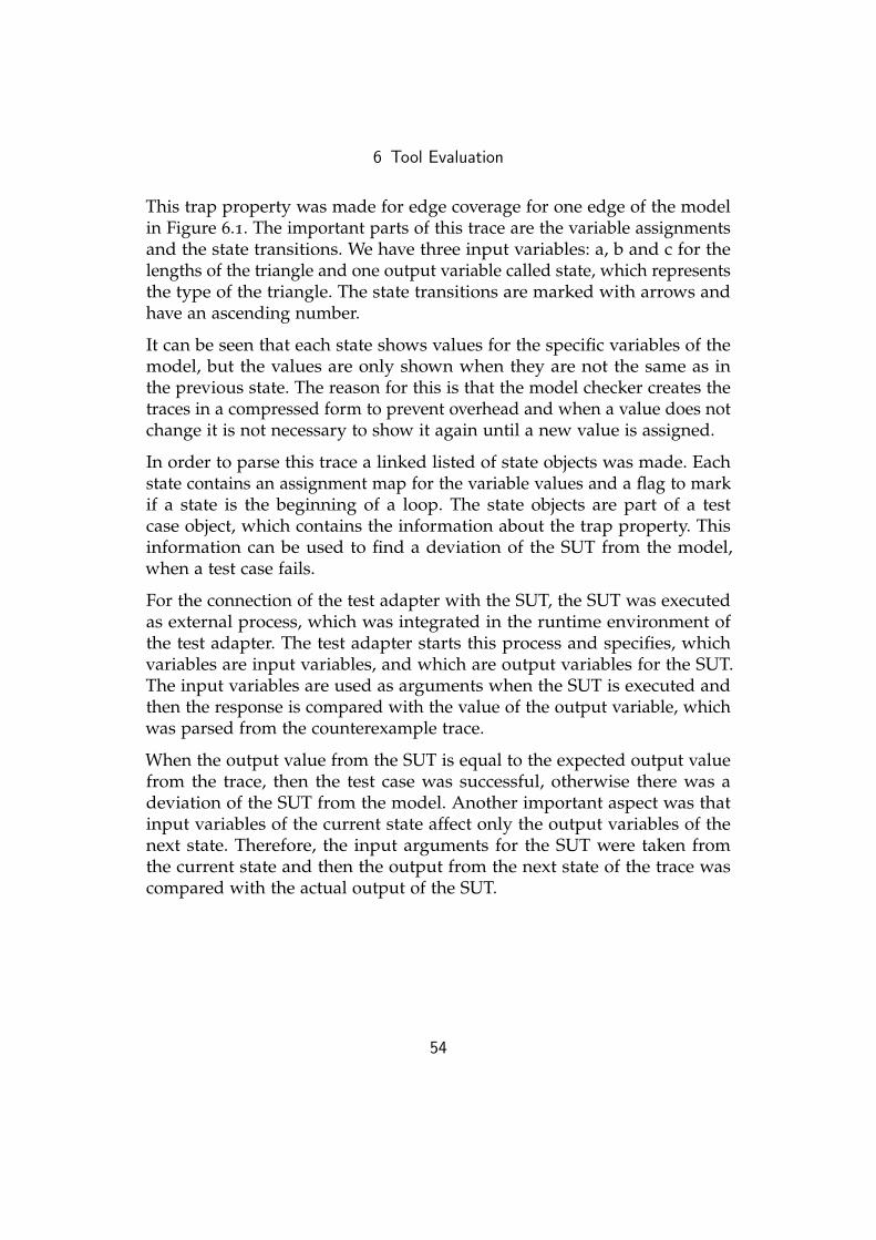
6 Tool Evaluation

This trap property was made for edge coverage for one edge of the modelin Figure 6.1. The important parts of this trace are the variable assignmentsand the state transitions. We have three input variables: a, b and c for thelengths of the triangle and one output variable called state, which representsthe type of the triangle. The state transitions are marked with arrows andhave an ascending number.

It can be seen that each state shows values for the specific variables of themodel, but the values are only shown when they are not the same as inthe previous state. The reason for this is that the model checker creates thetraces in a compressed form to prevent overhead and when a value does notchange it is not necessary to show it again until a new value is assigned.

In order to parse this trace a linked listed of state objects was made. Eachstate contains an assignment map for the variable values and a flag to markif a state is the beginning of a loop. The state objects are part of a testcase object, which contains the information about the trap property. Thisinformation can be used to find a deviation of the SUT from the model,when a test case fails.

For the connection of the test adapter with the SUT, the SUT was executedas external process, which was integrated in the runtime environment ofthe test adapter. The test adapter starts this process and specifies, whichvariables are input variables, and which are output variables for the SUT.The input variables are used as arguments when the SUT is executed andthen the response is compared with the value of the output variable, whichwas parsed from the counterexample trace.

When the output value from the SUT is equal to the expected output valuefrom the trace, then the test case was successful, otherwise there was adeviation of the SUT from the model. Another important aspect was thatinput variables of the current state affect only the output variables of thenext state. Therefore, the input arguments for the SUT were taken fromthe current state and then the output from the next state of the trace wascompared with the actual output of the SUT.

54

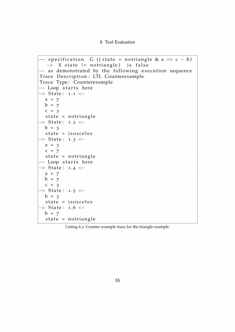
6 Tool Evaluation

−− s p e c i f i c a t i o n G ( ( s t a t e = n o t r i a n g l e & a <= c − b )−> X s t a t e != n o t r i a n g l e ) i s f a l s e

−− as demonstrated by the fol lowing execut ion sequenceTrace Descr ipt ion : LTL CounterexampleTrace Type : Counterexample−− Loop s t a r t s here−> S t a t e : 1 . 1 <−

a = 7

b = 7

c = 3

s t a t e = n o t r i a n g l e−> S t a t e : 1 . 2 <−

b = 3

s t a t e = i s o s c e l e s−> S t a t e : 1 . 3 <−

a = 3

c = 7

s t a t e = n o t r i a n g l e−− Loop s t a r t s here−> S t a t e : 1 . 4 <−

a = 7

b = 7

c = 3

−> S t a t e : 1 . 5 <−b = 3

s t a t e = i s o s c e l e s−> S t a t e : 1 . 6 <−

b = 7

s t a t e = n o t r i a n g l e

Listing 6.3: Counter example trace for the triangle example.

55

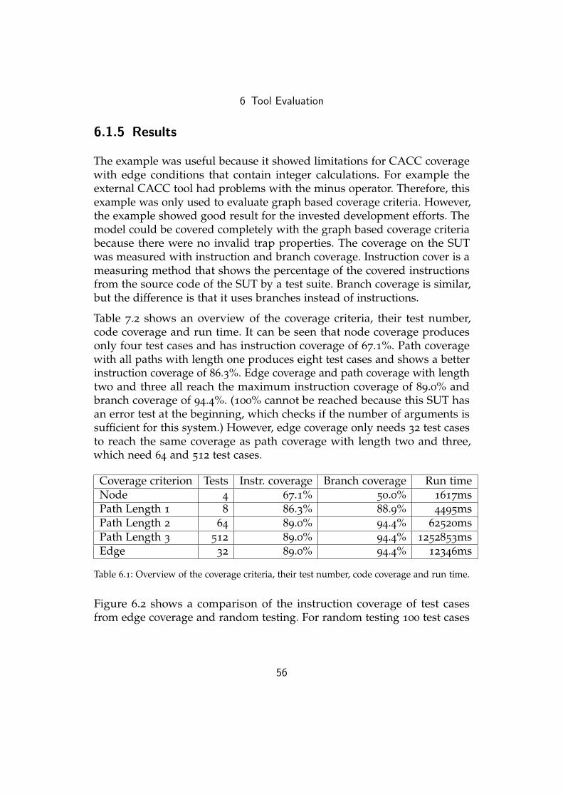
6 Tool Evaluation

6.1.5 Results

The example was useful because it showed limitations for CACC coveragewith edge conditions that contain integer calculations. For example theexternal CACC tool had problems with the minus operator. Therefore, thisexample was only used to evaluate graph based coverage criteria. However,the example showed good result for the invested development efforts. Themodel could be covered completely with the graph based coverage criteriabecause there were no invalid trap properties. The coverage on the SUTwas measured with instruction and branch coverage. Instruction cover is ameasuring method that shows the percentage of the covered instructionsfrom the source code of the SUT by a test suite. Branch coverage is similar,but the difference is that it uses branches instead of instructions.

Table 7.2 shows an overview of the coverage criteria, their test number,code coverage and run time. It can be seen that node coverage producesonly four test cases and has instruction coverage of 67.1%. Path coveragewith all paths with length one produces eight test cases and shows a betterinstruction coverage of 86.3%. Edge coverage and path coverage with lengthtwo and three all reach the maximum instruction coverage of 89.0% andbranch coverage of 94.4%. (100% cannot be reached because this SUT hasan error test at the beginning, which checks if the number of arguments issufficient for this system.) However, edge coverage only needs 32 test casesto reach the same coverage as path coverage with length two and three,which need 64 and 512 test cases.

Coverage criterion Tests Instr. coverage Branch coverage Run timeNode 4 67.1% 50.0% 1617msPath Length 1 8 86.3% 88.9% 4495msPath Length 2 64 89.0% 94.4% 62520msPath Length 3 512 89.0% 94.4% 1252853msEdge 32 89.0% 94.4% 12346ms

Table 6.1: Overview of the coverage criteria, their test number, code coverage and run time.

Figure 6.2 shows a comparison of the instruction coverage of test casesfrom edge coverage and random testing. For random testing 100 test cases

56

6 Tool Evaluation

were created with random numbers between 0 and 100, which is the samerange that was used in the model. These random numbers were used asvalues for the side lengths. It can be seen that random testing only reachesinstruction coverage of 72.2%, which is significantly lower than the 89%that are reached with edge coverage. For example random testing could notcover some condition cases and therefore it could not cover all instructions,edge coverage could cover all instructions except the ones for the errorhandling.

Edge Coverage Random Testing

Covered instructions

Uncovered instructions

89%

11%

72.2%

27.8%

Figure 6.2: Instruction coverage comparison of edge coverage with random testing withthe same number of test cases.

Figure 6.3 shows an overview of the time consumption of the tool executionsteps for different coverage criteria. It can be seen that the time consumptionfor model parsing is constant for all coverage criteria and the time for thetrap property generation is so small that it is insignificant compared to theother parts. Furthermore, the figure illustrates that the time for computationsof the model checker increases, when the number of test cases becomesbigger. Only when the number of test cases is very small, model checking isnot the major time consumption, otherwise it is so high that the other partsare insignificant.

57

6 Tool Evaluation

Node(4)

PathLength 1(8)

Edge(32)

PathLength 2(64)

0

20000

40000

60000

1,543 1,531 1,525 1,5561 3 3 473

2,961

10,818

62,520

Coverage Criterion (and Test Cases)

Run

tim

e[m

s]Model Parsing

Trap Property GenerationModel Checking

Figure 6.3: Time consumption of the tool execution steps for different coverage criteria.

6.2 Car Alarm Example

This car alarm system is based on the example state machine model whichwas presented by Aichernig [1]. The state machine model is shown inFigure 6.4. We made some modifications to the original model because notall complex features were necessary for a simple example. For instancethe time constraints are not included because they are not relevant for themodels in this thesis. However, this example is interesting because it hasseveral deterministic variables and it has many transitions with conditionsthat are dependent on other deterministic variables and it should be testedif the tool has problems with such features.

6.2.1 Functional Description

The car alarm example represents the security system of a car, which shouldbe able to detect a break-in, when a door is opened unjustified. In orderto activate the protection of the car, all doors need be closed and the car

58

6 Tool Evaluation

Figure 6.4: State machine model in UML of a car alarm system [1, p. 4].

59

6 Tool Evaluation

must be locked. Then, the alarm system is armed. In this state, an alarmis triggered when someone opens a door. The system has different alarmmodes. First, there is a sound alarm and afterwards there is a flash alarm.During these modes, the alarm can be deactivated by unlocking the car,which also makes the alarm system armed again. When the alarm is notdeactivated, the alarm system becomes silent after the alarm modes run out.In this state, the car is not protected. This behavior is represented with threedeterministic variables with case distinctions. One variable that indicateswhether the door is open or closed, one that reflects whether the car islocked or unlocked and one is for the state of the alarm system, which isused for the silent, armed and the alarmed states. The actions of closing,opening, locking and unlocking are represented by simple Boolean variables[1].

Listing 6.4 shows the described model. It can be seen that this model hasmore components and more complex than the first example, because thereare more deterministic variables and they are interconnected with eachother.

6.2.2 SUT

The implementation of the SUT required several case distinctions and aninput handling method. The case distinctions were used to reflect the statetransition of the alarm system. Additionally, the SUT required variablesto preserve the state. These variables were necessary to store the currentstate of the variables that represent the FSMs, so that the case distinctionsonly influence the output of the next state. This is important because thecase distinctions are dependent on the variable values of the previous state.Therefore, the value must not change in the middle of the case distinctions.

60

6 Tool Evaluation

MODULE main

VARdoClose : boolean ;doOpen : boolean ;doLock : boolean ;doUnLock : boolean ;

door : {open , c losed } ;lock : {unlocked , locked } ;alarmSystem : {unarmed , armed , soundAlarming ,

falshAlarming , s i l e n t } ;

ASSIGN

i n i t ( door ) := open ;next ( door ) :=

casedoor = open & doClose & ! doOpen : c losed ;door = closed & ! doClose & doOpen & lock != locked :

open ;door = open : open ;door = closed : c losed ;

esac ;

i n i t ( lock ) := unlocked ;next ( lock ) :=

caselock = unlocked & doLock & ! doUnLock & door =

closed : locked ;lock = locked & doUnLock & ! doLock : unlocked ;lock = unlocked : unlocked ;lock = locked : locked ;

esac ;

61

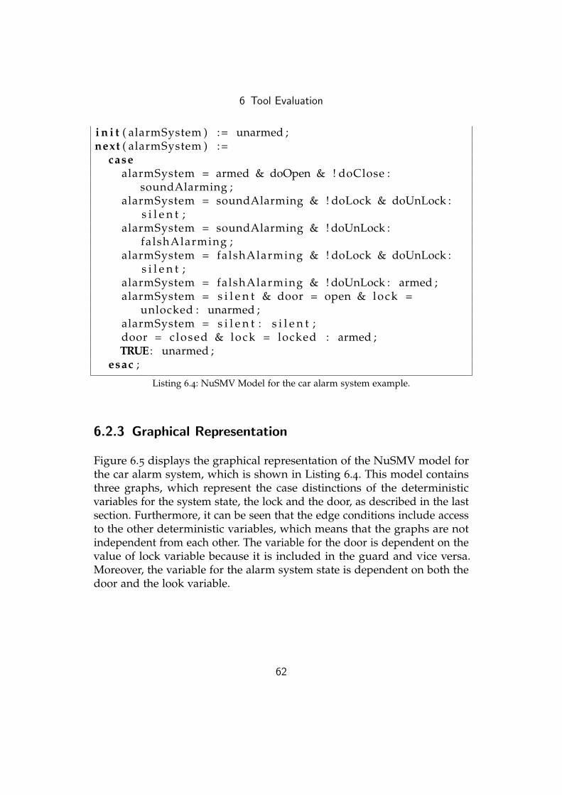
6 Tool Evaluation

i n i t ( alarmSystem ) := unarmed ;next ( alarmSystem ) :=

casealarmSystem = armed & doOpen & ! doClose :

soundAlarming ;alarmSystem = soundAlarming & ! doLock & doUnLock :

s i l e n t ;alarmSystem = soundAlarming & ! doUnLock :

falshAlarming ;alarmSystem = falshAlarming & ! doLock & doUnLock :

s i l e n t ;alarmSystem = falshAlarming & ! doUnLock : armed ;alarmSystem = s i l e n t & door = open & lock =

unlocked : unarmed ;alarmSystem = s i l e n t : s i l e n t ;door = closed & lock = locked : armed ;TRUE : unarmed ;

esac ;

Listing 6.4: NuSMV Model for the car alarm system example.

6.2.3 Graphical Representation

Figure 6.5 displays the graphical representation of the NuSMV model forthe car alarm system, which is shown in Listing 6.4. This model containsthree graphs, which represent the case distinctions of the deterministicvariables for the system state, the lock and the door, as described in the lastsection. Furthermore, it can be seen that the edge conditions include accessto the other deterministic variables, which means that the graphs are notindependent from each other. The variable for the door is dependent on thevalue of lock variable because it is included in the guard and vice versa.Moreover, the variable for the alarm system state is dependent on both thedoor and the look variable.

62

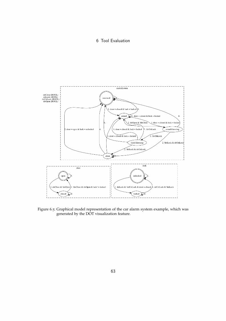
6 Tool Evaluation

Figure 6.5: Graphical model representation of the car alarm system example, which wasgenerated by the DOT visualization feature.

63

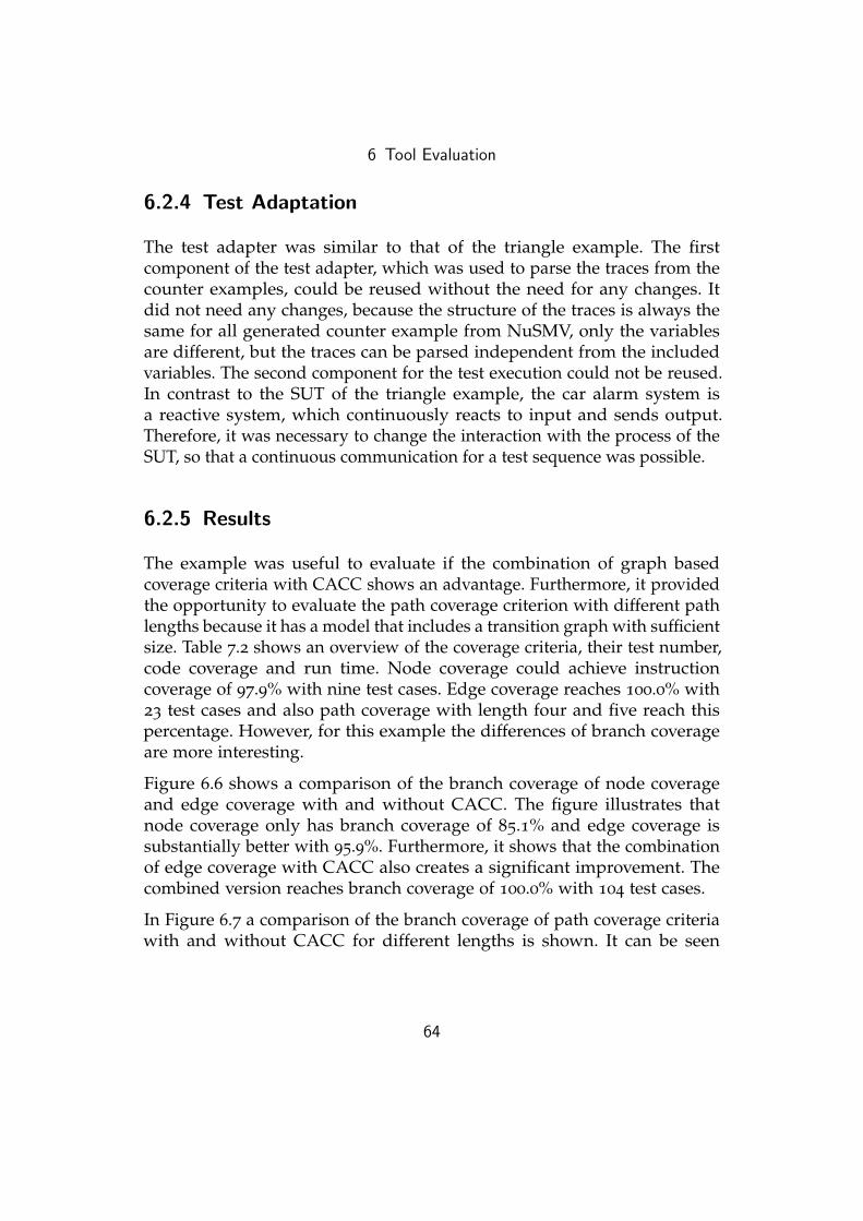
6 Tool Evaluation

6.2.4 Test Adaptation

The test adapter was similar to that of the triangle example. The firstcomponent of the test adapter, which was used to parse the traces from thecounter examples, could be reused without the need for any changes. Itdid not need any changes, because the structure of the traces is always thesame for all generated counter example from NuSMV, only the variablesare different, but the traces can be parsed independent from the includedvariables. The second component for the test execution could not be reused.In contrast to the SUT of the triangle example, the car alarm system isa reactive system, which continuously reacts to input and sends output.Therefore, it was necessary to change the interaction with the process of theSUT, so that a continuous communication for a test sequence was possible.

6.2.5 Results

The example was useful to evaluate if the combination of graph basedcoverage criteria with CACC shows an advantage. Furthermore, it providedthe opportunity to evaluate the path coverage criterion with different pathlengths because it has a model that includes a transition graph with sufficientsize. Table 7.2 shows an overview of the coverage criteria, their test number,code coverage and run time. Node coverage could achieve instructioncoverage of 97.9% with nine test cases. Edge coverage reaches 100.0% with23 test cases and also path coverage with length four and five reach thispercentage. However, for this example the differences of branch coverageare more interesting.

Figure 6.6 shows a comparison of the branch coverage of node coverageand edge coverage with and without CACC. The figure illustrates thatnode coverage only has branch coverage of 85.1% and edge coverage issubstantially better with 95.9%. Furthermore, it shows that the combinationof edge coverage with CACC also creates a significant improvement. Thecombined version reaches branch coverage of 100.0% with 104 test cases.

In Figure 6.7 a comparison of the branch coverage of path coverage criteriawith and without CACC for different lengths is shown. It can be seen

64

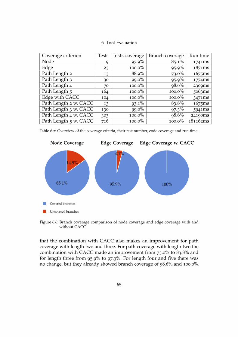
6 Tool Evaluation

Coverage criterion Tests Instr. coverage Branch coverage Run timeNode 9 97.9% 85.1% 1741msEdge 23 100.0% 95.9% 1871msPath Length 2 13 88.9% 73.0% 1675msPath Length 3 30 99.0% 95.9% 1774msPath Length 4 70 100.0% 98.6% 2309msPath Length 5 164 100.0% 100.0% 5063msEdge with CACC 104 100.0% 100.0% 3471msPath Length 2 w. CACC 13 93.1% 83.8% 1675msPath Length 3 w. CACC 130 99.0% 97.3% 5941msPath Length 4 w. CACC 303 100.0% 98.6% 24190msPath Length 5 w. CACC 716 100.0% 100.0% 181162ms

Table 6.2: Overview of the coverage criteria, their test number, code coverage and run time.

Node Coverage Edge Coverage Edge Coverage w. CACC

Covered branches

Uncovered branches

85.1%

14.9%

95.9%

4.1%

100%

Figure 6.6: Branch coverage comparison of node coverage and edge coverage with andwithout CACC.

that the combination with CACC also makes an improvement for pathcoverage with length two and three. For path coverage with length two thecombination with CACC made an improvement from 73.0% to 83.8% andfor length three from 95.9% to 97.3%. For length four and five there wasno change, but they already showed branch coverage of 98.6% and 100.0%.

65

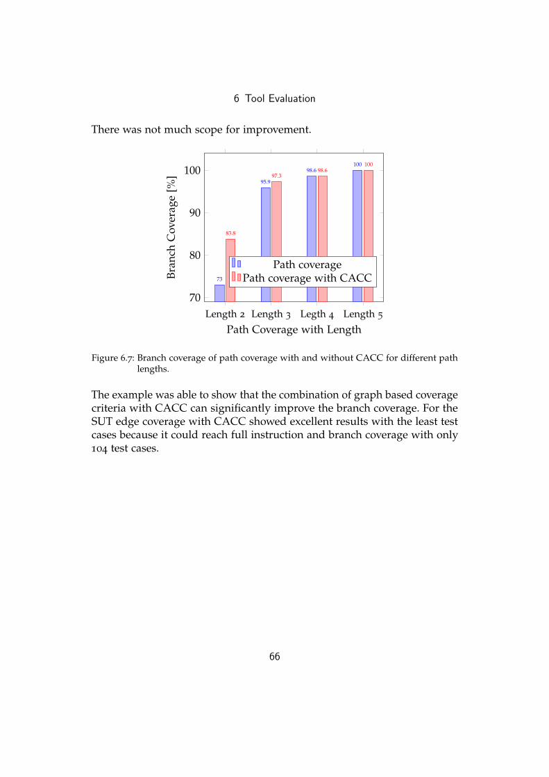
6 Tool Evaluation

There was not much scope for improvement.

Length 2 Length 3 Legth 4 Length 5

70

80

90

100

73

95.9

98.6100

83.8

97.398.6

100

Path Coverage with Length

Bran

chC

over

age

[%]

Path coveragePath coverage with CACC

Figure 6.7: Branch coverage of path coverage with and without CACC for different pathlengths.

The example was able to show that the combination of graph based coveragecriteria with CACC can significantly improve the branch coverage. For theSUT edge coverage with CACC showed excellent results with the least testcases because it could reach full instruction and branch coverage with only104 test cases.

66

6 Tool Evaluation

−− s p e c i f i c a t i o n G ( ( alarmSystem = unarmed & ( door =closed & lock = locked ) ) −> X ( ( alarmSystem = armed& ( doOpen = FALSE & doClose = FALSE) ) −> X

alarmSystem = soundAlarming ) ) i s f a l s e−− as demonstrated by the fol lowing execut ion sequenceTrace Descr ipt ion : LTL CounterexampleTrace Type : Counterexample−> S t a t e : 2 4 . 1 <−

doClose = FALSEdoOpen = FALSEdoLock = FALSEdoUnLock = FALSEdoor = openlock = unlockedalarmSystem = unarmed

−> S t a t e : 2 4 . 2 <−doClose = TRUE

−> S t a t e : 2 4 . 3 <−doLock = TRUEdoor = closed

−> S t a t e : 2 4 . 4 <−doClose = FALSEdoLock = FALSElock = locked

−− Loop s t a r t s here−> S t a t e : 2 4 . 5 <−

alarmSystem = armed−> S t a t e : 2 4 . 6 <−

Listing 6.5: Counter example trace for the car alarm system example.

67

7 Case Study

In this a case study we used our tool in order to generate test cases for a filecache implementation. The aim of this case study was to check if our toolis usable for real world examples. It was intended to check what problemsoccur, which coverage criteria are suitable for the given model, if there arecertain limitations for the trap property generation or any other problems.Furthermore, we will show performance data for the different coveragecriteria and how we measured the test quality. We will show how long thegeneration of the test cases takes and what coverage can be reached forcertain model and implementation parts.

7.1 SUT

The file cache that was used for the case study was implemented for aSecure Block Device (SBD) by Daniel Hein and C was used as programminglanguage. A SBD is a software component that uses symmetric cryptographyto ensure data confidentiality and integrity for persistent data storage. Inorder to increase the access speed to the secure data, the SBD splits thefile data into blocks and stores a configurable number of them in RAM. InRAM the blocks are unencrypted, but for the security goals of the SBD,a cryptographic nonce and an integrity tag are necessary. The SBD storescryptographic nonces and integrity tags bundled for a number of data blocksin separate blocks called management block. These management blockscontain the security meta data for a specific range of data blocks. A datablock can only be written or read, when the corresponding managementblock is also in the cache. Therefore, the cache implementation ensures thatfor each data block that is in the cache the corresponding managementblock must also be in the cache. When a data block is added to the cache or

68

7 Case Study

accessed, then also the according management block must be in the cache ormust be added. A management block can only be removed from the cache,when there are no dependent data blocks.

In order to make future requests faster, a cache stores certain blocks that areaccessed more often longer than blocks that are not used often. There aremany different approaches that can be used in order to decide which blocksshould be stored and how they are organized. This cache implementationuses the least recently used (LRU) algorithm. For this approach the blocksare sorted according to their access frequency and the block that was usedleast is on the last position. When a block is accessed and the block alreadyis in the cache, then its position in the cache is swapped with the position ofthe block in front of it. When there is an access to a block that is not in thecache, then one block must be removed so that this new block can be added.The LRU algorithm removes the block that was accessed least. This blockis on the last position. Although many actions happen in the backgroundin order to accomplish this behavior, the cache implementation details arebeyond the scope of this thesis.

7.2 Model Description

For this case study a model of the file cache implementation was given. Thismodel was developed by Franz Rock and Daniel Hein. The primary aim ofthe model is to reproduce the access behavior of the cache implementation,so it should reflect what happens when a certain cache position is accessedor when a block is searched that is not in the cache.

For the abstraction of the SUT we decided to limit the number of cachepositions to four. The size of the cache can be configured on the SUT, but alimited number is enough to test the access behavior. Another abstraction isthat only the type of a block is represented in the model, because modelingthe actual data is not feasible. A block can be a data or a management blockand both of them can be out of three ranges (x, y, z). A range representsa set of data blocks that have a common management block. For the SUTthe size of the ranges can be configured, but we decided to limit it for the

69

7 Case Study

model. In total, we have six different types: Dx, Dy, Dz for the data blocksand Mx, My, Mz for the corresponding management blocks.

The model of the cache implementation is divided in seven componentsrespectively deterministic variables: One is used for the representation ofthe actions that can occur on the system, four are used to reflect the contentof each cache position. Another one is used to select the cache position andthe last one is used to decide what type of entry should be added, whenthere is a cache miss. These variables are explained in more detail in thefollowing paragraphs.

The first variable is shown in Figure 7.1. (The guards are not shown in thisfigure because else the representations would be too big and therefore notviewable on a page.) This variable is the major component of the model,because it controls all actions. For example there are states that indicate thata new entry is added or that a cache block is accessed.

When the system is started only random data blocks are in the cache, whichwere selected with a non-deterministic init statement. The cache is startedwith this content because so it is not necessary to handle empty cachepositions separately. For the initialization of the cache there is an InitMNGTstate, which loads the management blocks for these data blocks. After thecache is initialized, the system goes in the idle state. In this state, it is possibleto access the cache. This can be done with a state called accessCacheBlock.When there is an access to block that already is in the cache then the systemreturns to the idle state, otherwise a new block must be loaded. For thisaction there is the fechNextD state, in which it is decided what type of blockshould be loaded. This decision is made by a separate deterministic variablethat is explained later. After this decision the system goes in a stated calledprocessD, in which it is checked if the corresponding management blockfor the data block is in the cache and if the block on the last position canbe removed or not. If there is a management block on this position, whichhas dependent data blocks, then this block cannot be removed and it isrepositioned. This action is done in the bump state. When the block on thelast position is free to drop, then the actual insertion happens in a statecalled insertD. In order to signal that a block was successfully added, thereis the insertDsuccess state. After this state the system returns in the idlestate. When the corresponding management block for the data block that

70

7 Case Study

needs to be added is not in the cache then the management block needsto be added first. The insertion of a management block is similar to theinsertion of a data block. It also happens in three states (processM, insertM,insertMsucsses). The only difference is that after the management block wassuccessfully inserted the system does not go back in the idle state, but inthe processD state so that the according data block can be added. The errorstate is only the default case. The system would go in this state, when noother transitions are possible, but normally this state cannot be reached.

The content of the cache positions and the required cache movements andreplacements for the different cache states are modeled by four deterministicvariables. Each of them represents the block type of one cache position.Together they control how the cache content is moved or added for thedifferent states. When there is an access to a cache position, then its contentis swapped with the content of the position in front of it.

The decision which cache position will be accessed is made by variable calledCacheIdx when the system is in the idle state. This decision is only limitedby the fact that only data blocks can be accessed, because managementblocks are not usable by the user they only provide security informationfor the data blocks and are used in the background. In order to find outon which position there are data blocks, the variables for the cache contentare checked. The index of one position with a data block is selected non-deterministically or minus one is selected. When this variable is set to minusone, it represents a cache miss. So then a block that is not in the cache isaccessed and it must be loaded into the cache.

Another variable called newentry was used to decide, which type of entrywill be added, when there is a cache miss. The choice is made when thesystem is in the fetchNextD state and then the value stays the same untilthe system is in this state again. Only data blocks can be chosen, becausemanagement blocks cannot be directly accessed and the possible values are:Dx, Dy and Dz.

Table 7.1 shows an example for the access behavior of the cache. When thecache is started there are random data blocks in the cache. In InitMNGTstate the management blocks are loaded for these data blocks. After theinitialization several accesses are made to the cache, some of them produce acache miss and then new entries are loaded in the cache. The states between

71

7 Case Study

Figure 7.1: Cache model variable for the global system state, which shows what action iscurrently in progress.

72

7 Case Study

the cache accesses are not shown in this table because this would producetoo much overhead, but it can be seen how the cache content is changedwhen an access occurs or when new entries are loaded.

action cache0 cache1 cache2 cache3

when started Dx Dx Dx DxInitMNGT Dx Dx Dx Mx

accessCacheBlock Dx Mx Dz MzCacheIdx = -1, newentry = Dz

accessCacheBlock Mx Dx Dz MzCacheIdx = 0

accessCacheBlock Mx Dz Dx MzCacheIdx = 1

accessCacheBlock Dx Mz Mx DzCacheIdx = -1, newentry = Dx

accessCacheBlock Mz Dx Mx DxCacheIdx = 0

accessCacheBlock Dx Mx Dx DxCacheIdx = -1, newentry = Dx

accessCacheBlock Mx Dx Dx DxCacheIdx = 0

Table 7.1: Example for the access behavior of the cache. The actions with the requiredparameters and the resulting cache content are demonstrated in this table.

7.3 Test Adapter

The test adapter implementation was different from the previous testadapters from the example projects. Only the parsing process of the counterexample traces was the same, but the test cases were not directly execut-ing after they were parsed. Instead, we used the parsed traces to generatesource code in the form of function calls to wrapper functions with testdata as arguments. These wrapper functions were used to perform the testexecution and to check if the expected cache content matches the actualcache content after the execution. The source code was injected in a testclass of the SUT, which includes these wrapper functions. Listing 7.1 showsan example of a generated test case. The example was already used todemonstrate the access behavior of the model, which is shown in Table 7.1

73

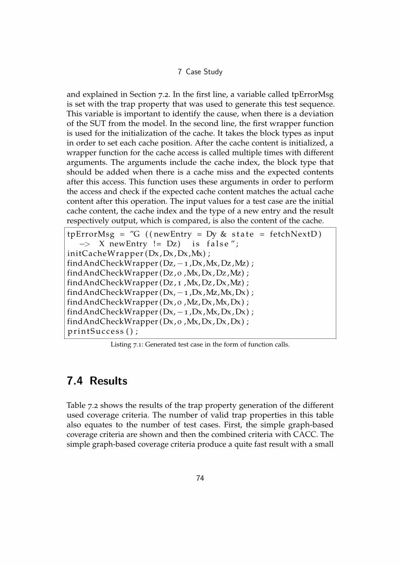
7 Case Study

and explained in Section 7.2. In the first line, a variable called tpErrorMsgis set with the trap property that was used to generate this test sequence.This variable is important to identify the cause, when there is a deviationof the SUT from the model. In the second line, the first wrapper functionis used for the initialization of the cache. It takes the block types as inputin order to set each cache position. After the cache content is initialized, awrapper function for the cache access is called multiple times with differentarguments. The arguments include the cache index, the block type thatshould be added when there is a cache miss and the expected contentsafter this access. This function uses these arguments in order to performthe access and check if the expected cache content matches the actual cachecontent after this operation. The input values for a test case are the initialcache content, the cache index and the type of a new entry and the resultrespectively output, which is compared, is also the content of the cache.

tpErrorMsg = ”G ( ( newEntry = Dy & s t a t e = fetchNextD )−> X newEntry != Dz) i s f a l s e ” ;

initCacheWrapper (Dx , Dx , Dx ,Mx) ;findAndCheckWrapper (Dz,−1 ,Dx ,Mx, Dz ,Mz) ;findAndCheckWrapper (Dz , 0 ,Mx, Dx , Dz ,Mz) ;findAndCheckWrapper (Dz , 1 ,Mx, Dz , Dx ,Mz) ;findAndCheckWrapper (Dx,−1 ,Dx ,Mz,Mx, Dx) ;findAndCheckWrapper (Dx, 0 ,Mz, Dx ,Mx, Dx) ;findAndCheckWrapper (Dx,−1 ,Dx ,Mx, Dx , Dx) ;findAndCheckWrapper (Dx, 0 ,Mx, Dx , Dx , Dx) ;p r i n t S u c c e s s ( ) ;

Listing 7.1: Generated test case in the form of function calls.

7.4 Results

Table 7.2 shows the results of the trap property generation of the differentused coverage criteria. The number of valid trap properties in this tablealso equates to the number of test cases. First, the simple graph-basedcoverage criteria are shown and then the combined criteria with CACC. Thesimple graph-based coverage criteria produce a quite fast result with a small

74

7 Case Study

number of invalid trap properties. Nevertheless, the combined coveragecriteria with CACC have really a lot of invalid trap properties and only alimited number of valid once. The cause of this problem was analyzed. It wasmeasured, which model components have transitions that were not covered.It turns out that especially the variables for the cache content have problems.These variables have basically the same transitions and therefore the sameproblems. The assignment generation with the CACC tool produced ahigh number of assignment combinations that are not applicable on themodel, because they are prohibited from define restrictions as explained inSection 5.9. However, the other model components worked well with CACCcoverage. For the problematic variables it might be better to use a simplegraph-based coverage like edge coverage.

Coverage criterion all TPs valid TPs invalid TPs Run timeNode 46 45 1 3min 13sEdge 530 357 173 18min 39sPath Length 1 330 248 82 10min 37sPath Length 2 15629 451 15178 27h 31minEdge with CACC 7584 1328 6256 1h 49minPath Length 1 with CACC 5474 1108 4366 57min 56s

Table 7.2: Overview of the coverage criteria, their trap properties (TPs) and run time.

Figure 7.2 shows a comparison of the runtime of the used coverage criteria.The major time consumption is caused by the model checker, the runtimefor the other tasks is neglectable. This was explained in Section 6.1.5. It canbe seen that node coverage only takes about three minutes and generates 45

test cases. Path coverage created 248 test cases in about 10 minutes. However,path coverage with length one is not interesting because it cannot reachmost model states and with length two it already took over 27 hours. Pathcoverage with a usable length was impracticable for this model, because itincludes many variables with a high number of edges and multiple initialand target nodes, which makes the number of theoretically possible pathsand thereby the computation time impracticable. Edge coverage took about19 minutes to generate 357 test cases and the combined version with CACCtook about one hour and 11 minutes to generate 1328 test cases.

For the analysis of the test quality the percentage of line coverage and branchcoverage were measured on the SUT. The gnu coverage tool gcov [4] was

75

7 Case Study

used to perform this measure for the involved functions. Figure 7.3 showsa comparison of the coverage criteria and their line and branch coverage.Node coverage reached line coverage of 87.1% and branch coverage of90.48% on the SUT with 45 test cases. Edge coverage could improve the linecoverage to 89.52% and used 357 test cases. Path coverage with length twoalso showed line coverage of 89.52% and branch coverage of 90.48% with451 test cases. The combination of edge coverage with CACC produced 1328

test cases and showed also line coverage of 89.52% and branch coverage of90.48%. So node coverage was not as effective as edge coverage, but edgecoverage and edge coverage with CACC showed no difference regardingline and branch coverage.

The model coverage was analyzed by visually highlighting the coveredmodel parts, when a valid trap property could be produced. For exampleafter the trap property generation was finished a model visualization withcolored transitions was produced. In this visualization color was applied tohighlight the transitions, for which it was possible to generate a test case.We compared the highlighted transitions and states for edge coverage withand without CACC. This comparison was especially helpful to find thecause of the high number of invalid trap properties with CACC, but it alsoshowed that CACC worked well for the other model parts.

Overall, edge coverage reached the best coverage on the SUT with theleast number of test cases. Edge coverage combined with CACC showed abetter coverage for the edge conditions of most variables, only for certainvariables, simple edge coverage produced trap properties with a bettermodel coverage. Furthermore, an old version of the cache implementationwith a bug was tested. The bug occurred when a data block was addedand the corresponding management block was in the last position. When amanagement block is in the last position and there are no correspondingdata blocks in the cache, then this block can be dropped. However, whenthe new block that needs to be added is dependent on this managementblock, then it is wrong to delete this block first because a data block alwaysneeds its corresponding management block in the cache. This bug, whichwas only found after weeks of manual testing, could be found immediatelyby the generated test cases. If the tool would have been used earlier, it couldhave saved a lot of debugging effort.

76

7 Case Study

Node(45)

PathLength 1(248)

Edge(357)

PathLength 1 w.CACC(1108)

Edge w.CACC(1328)

0

2

4

6

·106

1.93 · 1056.37 · 105

1.12 · 106

3.48 · 106

6.56 · 106

Coverage method (and Test Cases)

Run

tim

e[m

s]

Figure 7.2: Run time comparison of the different coverage methods.

Node45 TCs

Edge357 TCs

Edge w. CACC1328 TCs

87

88

89

90

87.1

89.52 89.52

90.48 90.48 90.48

Coverage method and Test Cases

Cod

eC

over

age

[%]

Line coverageBranch coverage

Figure 7.3: Comparison of the coverage criteria and their line and branch coverage.

77

8 Outlook

There are many features and possible extensions for the developed tool,which could provide further research topics. The tool could be extendedto support models that include further features, for instance array support,more mathematical operations for the CACC tool, like multiplication anddivision, and full integer support would be options.

Moreover, an interesting extension would be the implementation of morecoverage criteria. For example there are a few more logic-based criterialike RACC that could be combined with the implemented graph-basedcoverage criteria. Different combination methods of coverage criteria couldbe considered and evaluated and it could be checked if they show betterresults.

Another issue is the performance of the test case generation with the tool.Although the trap property generation works quite fast, the generation ofthe counter examples for the trap properties with the model checker needsa lot of time, when a model has many transition. For example path coveragewith length two took about 27 hours for the model from the case studyand also the other coverage criteria took some time to compute the trapproperties, which can be seen in Table 7.2. There are optimizations thatcould be done in order to improve the performance. For example, the trapproperties could be formulated in a different way, for example with CTL, oranother model checker could be used and there are many other approachesas described by Fraser [11].

As already described in the case study due to the define restrictions andthe limitation for the distinction of the CACC assignments, many counterexamples are invalid and therefore not useful to generate test cases, butthey also contribute to the computation time. There are certain actions thatcan reduce the number of invalid trap properties. For example, the external

78

8 Outlook

CACC tool could add a mark to the test assignments that make the inputformula true in order to distinguish them the assignments for a false case.Then, it would be possible to reduce the number of trap properties, becauseit would not be necessary to create them for both cases.

Another improvement would be parallelization of the counter examplegeneration with the model checker. When multiple model checker processesare used for the application of the trap properties then depending on thegiven hardware it would also make the generation faster.

An extension for online testing would also be interesting. The differencebetween normal (offline) and online testing is that the test cases are imme-diately executed on the SUT when they are generated. It is not necessaryto store all test cases and execute them after the generation is finished, butthe execution is directly combined with the generation. The advantage ofthis approach is that the storage of test cases does not become a bottleneckand also it is possible to receive a direct feedback for the current test cases.When there is a problem we can find it faster, because we do not have towait until the generation of all test cases is finished [21, p. 80ff.].

Another possible research topic could be test suite minimization. The gener-ated test cases from the tool are not free from overlap. For example, when atest case was generated for a certain graph components, then it might alsoinclude steps that could be used to test other components. This can makeother test cases redundant. If it is possible to find these test cases, it canincrease the performance of the tool and reduce the number of required testcases. Test case minimization is a similar approach that also can increase theperformance. The difference is that not the number of test cases is reduced,but the length of the test cases. NuSMV creates counter example tracesthat contain some overhead because it tries to find loops for the traces. Apossible way to minimize the test cases respectively traces is to cut the tracesof, when the property that needs to be checked is reached in the trace.

79

9 Conclusion

In this thesis an automatic test case generation approach was presented thatcombines graph-based coverage criteria with logic-based coverage criteriaand a tool was developed that implements this approach.

First, different coverage criteria were evaluated and implemented to testhow the perform for number of example models.

In order to automatically generate test cases a tool was implemented thattakes a NuSMV model as input, then computes trap properties according toa selected coverage criteria, and uses a model checker to compute abstracttest cases for these trap properties. These abstract test cases were parsedby a test adapter and executed as concrete test cases on the SUT. Then,combination methods were developed by including an existing tool forCACC test data generation and applying this test data to graph-basedcoverage criteria.

These combination methods and the tool were analyzed with several smalltest projects. The triangle example could reach statement coverage of 89.0%and branch coverage of 94.4% with edge coverage. For the car alarm systemit could be shown that the combination of edge coverage with CACCincreased the branch coverage from 95.9% to 100% and also path coveragecould be improved with this combination.

Then, the approach was evaluated with a case study, where it was appliedto a real world project with a bigger model. It could be shown that edgecoverage reaches line coverage of 89.52% and branch coverage of 90.48%for the SUT with the least number of test cases. Edge coverage with CACCshowed the same coverage for the SUT and could increase the coverage formost model parts. However, for some model parts CACC could not increasethe coverage, because variable limitations in the define part restricted some

80

9 Conclusion

generated variable assignments for CACC. Other models without suchlimitations could even show better results, but the generated test casesstill showed a high code coverage and were able to find a bug in an olderversion of the implementation. Furthermore, the automated tool providesthe advantage that many test cases can be generated in a relatively shorttime, without the need to be expert for coverage criteria and with littlemanual effort.

81

List of Figures

1.1 Schematic component overview. . . . . . . . . . . . . . . . . . 6

2.1 Coverage Explanation Example. . . . . . . . . . . . . . . . . . 15

5.1 UML Class Diagram of the Model Structure. . . . . . . . . . . 34

5.2 DOT Visualization Example. . . . . . . . . . . . . . . . . . . . . 36

6.1 Triangle Example. . . . . . . . . . . . . . . . . . . . . . . . . . . 53

6.2 Instruction coverage comparison of edge coverage with ran-dom testing with the same number of test cases. . . . . . . . . 57

6.3 Time consumption of the tool execution steps for differentcoverage criteria. . . . . . . . . . . . . . . . . . . . . . . . . . . 58

6.4 Car Alarm UML Model. . . . . . . . . . . . . . . . . . . . . . . 59

6.5 Car Alarm System. . . . . . . . . . . . . . . . . . . . . . . . . . 63

6.6 Branch coverage comparison of node coverage and edge cov-erage with and without CACC. . . . . . . . . . . . . . . . . . . 65

6.7 Branch coverage of path coverage with and without CACCfor different path lengths. . . . . . . . . . . . . . . . . . . . . . 66

7.1 Cache model variable for the global system state. . . . . . . . 72

7.2 Run time comparison of the different coverage methods. . . . 77

7.3 Comparison of the coverage criteria and their line and branchcoverage. . . . . . . . . . . . . . . . . . . . . . . . . . . . . . . . 77

82

Listings

2.1 NuSMV test model for the illustration of coverage criteria. . . 15

2.2 Trap properties for edge coverage. . . . . . . . . . . . . . . . . 17

2.3 Trap properties for path coverage. . . . . . . . . . . . . . . . . 18

5.1 DOT output of a small access policy example. . . . . . . . . . 35

5.2 Counter example in the form of a trace from NuSMV process. 38

5.3 Generated test case assignments from the CACC tool. . . . . . 41

5.4 Trap properties for the CACC assignments. . . . . . . . . . . . 42

6.1 SUT for the triangle example. . . . . . . . . . . . . . . . . . . . 51

6.2 NuSMV model for the triangle exmaple. . . . . . . . . . . . . 52

6.3 Counter example trace for the triangle example. . . . . . . . . 55

6.4 NuSMV Model for the car alarm system example. . . . . . . . 61

6.5 Counter example trace for the car alarm system example. . . 67

7.1 Generated test case in the form of function calls. . . . . . . . . 74

83

Bibliography

[1] Bernhard K Aichernig. “Model-Based Mutation Testing of ReactiveSystems.” In: Theories of Programming and Formal Methods. Springer,2013, pp. 23–36 (cit. on pp. 49, 58–60).

[2] Paul Ammann, Jeff Offutt, and Wuzhi Xu. “Coverage criteria for statebased specifications.” In: Formal methods and testing. Springer, 2008,pp. 118–156 (cit. on pp. 3–5, 14, 16–24, 26).

[3] Gilles Bernot, Marie Claude Gaudel, and Bruno Marre. “Softwaretesting based on formal specifications: a theory and a tool.” In: SoftwareEngineering Journal 6.6 (1991), pp. 387–405 (cit. on p. 25).

[4] Steve Best. “Analyzing code coverage with gcov.” In: Linux Magazine(2003), pp. 43–50 (cit. on p. 75).

[5] Roderick Bloem, Karin Greimel, Robert Koenighofer, and Franz Roeck.“Model-Based MCDC Testing of Complex Decisions for the Java CardApplet Firewall.” In: VALID 2013, The Fifth International Conference onAdvances in System Testing and Validation Lifecycle. 2013, pp. 1–6 (cit. onpp. 6, 19, 21–23, 25, 28, 31, 40).

[6] Roberto Cavada, Alessandro Cimatti, Charles Arthur Jochim, GavinKeighren, Emanuele Olivetti, Marco Pistore, Marco Roveri, and AndreiTchaltsev. Nusmv 2.4 user manual. 1998 (cit. on pp. 43, 47).

[7] Roberto Cavada, Alessandro Cimatti, Gavin Keighren, EmanueleOlivetti, Marco Pistore, and Marco Roveri. “NuSMV 2.2 Tutorial.”In: ITC-irst-Via Sommarive 18 (2004), p. 38055 (cit. on pp. 14, 43, 45).

[8] John J Chilenski. An investigation of three forms of the modified conditiondecision coverage (MCDC) criterion. Tech. rep. DTIC Document, 2001

(cit. on pp. 24, 26).

84

Bibliography

[9] Alessandro Cimatti, Edmund Clarke, Fausto Giunchiglia, and MarcoRoveri. “NuSMV: a new symbolic model checker.” In: InternationalJournal on Software Tools for Technology Transfer 2.4 (2000), pp. 410–425

(cit. on p. 13).

[10] John Ellson, Emden Gansner, Lefteris Koutsofios, Stephen C North,and Gordon Woodhull. “Graphviz—open source graph drawing tools.”In: Graph Drawing. Springer. 2002, pp. 483–484 (cit. on p. 33).

[11] Gordon Fraser. “Automated Software Testing with Model Checkers.”PhD thesis. Institute for Softwaretechnology Graz University of Tech-nology, Oct. 2007 (cit. on pp. 1, 25, 78).

[12] Gordon Fraser, Franz Wotawa, and Paul E Ammann. “Testing withmodel checkers: a survey.” In: Software Testing, Verification and Reliabil-ity 19.3 (2009), pp. 215–261 (cit. on pp. 3, 4, 14, 16–18, 25).

[13] Emden R Gansner. Drawing graphs with Graphviz. Tech. rep. GraphVizWebSite, 2009. url: http://www.graphviz.org/pdf/libguide.pdf(cit. on p. 33).

[14] Siamak Haschemi. NuSMV-Tools (Tools for the model checker NuSMV).Apr. 2012. url: https://code.google.com/a/eclipselabs.org/p/nusmv-tools/ (cit. on p. 32).

[15] Mats PE Heimdahl, Sanjai Rayadurgam, and Willem Visser. “Spec-ification centered testing.” In: Proceedings of the Second InternationalWorkshop on Automated Program Analysis, Testing and Verification. 2001

(cit. on pp. 2, 12).

[16] Anders Hessel and Paul Pettersson. “Cover-A test-case generation toolfor timed systems.” In: Testing of Software and Communicating Systems(2007), pp. 31–34 (cit. on p. 26).

[17] Hyoung Seok Hong, Sung Deok Cha, Insup Lee, Oleg Sokolsky,and Hasan Ural. “Data flow testing as model checking.” In: SoftwareEngineering, 2003. Proceedings. 25th International Conference on. IEEE.2003, pp. 232–242 (cit. on p. 25).

[18] Michael Huth and Mark Ryan. Logic in Computer Science: Modellingand reasoning about systems. Cambridge University Press, 2004 (cit. onp. 11).

85

Bibliography

[19] Eleftherios Koutsofios, Stephen North, et al. Drawing graphs with dot.Tech. rep. Technical Report 910904-59113-08TM, AT&T Bell Laborato-ries, Murray Hill, NJ, 1991 (cit. on p. 33).

[20] Jussi Lahtinen. Simplification of NuSMV Model Checking Counter Ex-amples. 2008. url: http://www.tcs.hut.fi/Studies/T-79.5001/reports/laht08simcex.pdf (cit. on pp. 2, 10, 11, 26).

[21] Kim G Larsen, Marius Mikucionis, and Brian Nielsen. Online testing ofreal-time systems using uppaal. Springer, 2005 (cit. on p. 79).

[22] Jeff Offutt, Shaoying Liu, Aynur Abdurazik, and Paul Ammann. “Gen-erating test data from state-based specifications.” In: Software Testing,Verification and Reliability 13.1 (2003), pp. 25–53 (cit. on pp. 3, 25, 26).

[23] Thomas J. Ostrand and Marc J. Balcer. “The category-partition methodfor specifying and generating fuctional tests.” In: Communications ofthe ACM 31.6 (1988), pp. 676–686 (cit. on p. 25).

[24] Jan Kohnlein Peter Friese Sven Efftinge. Build your own textual DSLwith Tools from the Eclipse Modeling Project. Apr. 2008. url: http://www.eclipse.org/articles/article.php?file=Article-BuildYourOwnDSL/

index.html (cit. on p. 32).

[25] Amir Pnueli. “The temporal logic of programs.” In: Foundations ofComputer Science, 1977., 18th Annual Symposium on. IEEE. 1977, pp. 46–57 (cit. on p. 10).

[26] Martin Pol, Tim Koomen, and Andreas Spillner. “Management undOptimierung des Testprozesses.” In: Heidelberg: dpunkt. verlag (2000)(cit. on p. 1).

[27] M Prasanna, SN Sivanandam, R Venkatesan, and R Sundarrajan. “Asurvey on automatic test case generation.” In: Academic Open InternetJournal 15.part 6 (2005) (cit. on p. 2).

[28] Special C. of RTCA. DO-178C, Software Considerations in Airborne Sys-tems and Equipment Certification. 2011 (cit. on p. 3).

[29] Jan Tretmans. “Model based testing with labelled transition systems.”In: Formal methods and testing. Springer, 2008, pp. 1–38 (cit. on p. 2).

86

Bibliography

[30] Mark Utting, Alexander Pretschner, and Bruno Legeard. “A taxonomyof model-based testing approaches.” In: Software Testing, Verificationand Reliability (STVR) 22.5 (Aug. 2012), pp. 297–312. issn: 0960-0833.doi: 10.1002/stvr.456 (cit. on pp. 1, 2).

[31] Margus Veanes, Colin Campbell, Wolfgang Grieskamp, WolframSchulte, Nikolai Tillmann, and Lev Nachmanson. “Model-based test-ing of object-oriented reactive systems with Spec Explorer.” In: Formalmethods and testing. Springer, 2008, pp. 39–76 (cit. on p. 26).

[32] Stephan Weißleder. “Test models and coverage criteria for automaticmodel-based test generation with UML state machines.” PhD thesis.Humboldt University of Berlin, 2010 (cit. on pp. 3, 25).

[33] Elaine Weyuker, Tarak Goradia, and Ashutosh Singh. “Automaticallygenerating test data from a Boolean specification.” In: IEEE Transac-tions on Software Engineering 20.5 (1994), pp. 353–363 (cit. on p. 25).

87