Automatic registration of aerial imagery with untextured 3D LiDAR models

Min Ding, Kristian Lyngbaek and Avideh ZakhorUniversity of California, Berkeley

Electrical Engineering and Computer Science Department{dingm, kristian, avz }@eecs.berkeley.edu

Abstract

A fast 3D model reconstruction methodology is desir-able in many applications such as urban planning, train-ing, and simulations. In this paper, we develop an au-tomated algorithm for texture mapping oblique aerial im-ages onto a 3D model generated from airborne Light De-tection and Ranging (LiDAR) data. Our proposed systemconsists of two steps. In the first step, we combine van-ishing points and global positioning system aided inertialsystem readings to roughly estimate the extrinsic parame-ters of a calibrated camera. In the second step, we re-fine the coarse estimate of the first step by applying a se-ries of processing steps. Specifically, We extract 2D cor-ners corresponding to orthogonal 3D structural corners asfeatures from both images and the untextured 3D LiDARmodel. The correspondence between an image and the 3Dmodel is then performed using Hough transform and gen-eralized M-estimator sample consensus. The resulting 2Dcorner matches are used in Lowe’s algorithm to refine cam-era parameters obtained earlier. Our system achieves91%correct pose recovery rate for 90 images over the downtownBerkeley area, and overall61% accuracy rate for 358 im-ages over the residential, downtown and campus portionsof the city of Berkeley.

1. Introduction

3D models are needed in many applications such as ur-ban planning, architecture design, telecommunication net-work design, cartography and virtual fly/drive-through. Dueto their significance and vast potential, fast and automatedmodel reconstruction has drawn a great deal of attention andeffort from many researchers in the last three decades. How-ever, most existing approaches lack either accuracy or thescalability needed for creating textured models of large ur-ban areas. Even though model geometry can be quickly andautomatically generated from aerial images or Light Detec-tion and Ranging (LiDAR) data [15], registering imagerywith a 3D model for texture mapping purposes is consider-

ably less automated and more time-consuming; this is dueto lengthy manual correspondence between a 3D model andimages, or computationally intensive automated pose recov-ery algorithms. For instance, the pose recovery algorithmproposed by Frueh et al. [6] for texture mapping obliqueaerial imagery onto untextured 3D models takes approxi-mately 20 hours per image. In this paper, we develop a fast,automated camera pose recovery algorithm for texture map-ping oblique aerial imagery onto pre-existing untextured 3Dmodels obtained via various sensing modalities such as Li-DAR. We believe that such algorithms are the key to fast,automated 3D airborne modeling of large scale environ-ments.

There have been a number of approaches to automatedtexture mapping of 3D models. Stomas and Liu have de-veloped texture mapping for ground based multiview im-ages [11, 17]. They use vanishing points and rectangularparallelepipeds on building facades for matching featuresbetween LiDAR data and images in order to identify cam-era parameters. They further refine the parameters by 3Dpoint cloud correspondence between the LiDAR data andthe sparse point cloud generated from multiview geometry.Their algorithm requires multiview imagery, and runs intodifficulties if there are no two pairs of correctly matchedparallelepipeds. They also take advantage of the groundbased image acquisition where clear parallelism and orthog-onality of building contours are visible with little occlusion.By contrast in our application, it is desirable to develop anapproach which uses single view, and can handle complexurban scenes with significant occlusions.

In video based texture mapping, Hsu et al. first use thetracked features for inter-frame pose prediction, and refinethe pose by aligning the projected 3D model lines to thosein images [8]. Neumann et al. follow a similar idea byimplementing an extended Kalman filter to perform inter-frame camera parameter tracking using point and line fea-tures [14]. Both methods can lose track in situations withlarge pose prediction error due to occlusions. Zhao et al. in-stead use iterative closest point algorithm to align the pointcloud from video to that from a range sensor [20]. However,

1

Step2: Fine camera pose estimation

Perspective

projection

Step1: Coarse camera pose estimation

GPS and

compass

measurement

Coarse

estimate of

camera

pose

Vertical vanishing point

detection

Non-vertical vanishing points

detection

Aerial

image

Vanishing point detection

LIDAR

data

2D corner detection

from DSM

Aerial

image

2D corner detection

from image

Feature point

correspondence

Hough transform on

rotation angles

Generalized M-estimator

Sample Consensus

(GMSAC)

DSM-image 2D

corner

correspondence

Lowe’s camera pose

recovery algorithm

Fine estimate of

camera pose

pitch and roll angles

x, y, z and

yaw angle

~ 1000 corners

~ 1000

corners

Generate putative

matches based on corner

descriptor and distance

~ 3000

matches

~ 200 matches

~ 100

matches

pitch and roll angles

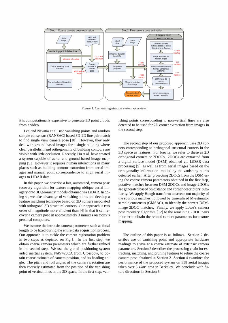
Figure 1.Camera registration system overview.

it is computationally expensive to generate 3D point cloudsfrom a video.

Lee and Nevatia et al. use vanishing points and randomsample consensus (RANSAC) based 3D-2D line pair matchto find single view camera pose [10]. However, they onlydeal with ground based images for a single building whereclear parallelism and orthogonality of building contours arevisible with little occlusion. Recently, Hu et al. have createda system capable of aerial and ground based image map-ping [9]. However it requires human interactions in manyplaces such as building contour extraction from aerial im-ages and manual point correspondence to align aerial im-ages to LiDAR data.

In this paper, we describe a fast, automated, camera poserecovery algorithm for texture mapping oblique aerial im-agery onto 3D geometry models obtained via LiDAR. In do-ing so, we take advantage of vanishing points and develop afeature matching technique based on 2D corners associatedwith orthogonal 3D structural corners. Our approach is twoorder of magnitude more efficient than [4] in that it can re-cover a camera pose in approximately 3 minutes on today’spersonal computers.

We assume the intrinsic camera parameters such as focallength to be fixed during the entire data acquisition process.Our approach is to tackle the camera registration problemin two steps as depicted on Fig.1. In the first step, weobtain coarse camera parameters which are further refinedin the second step. We use the global positioning systemaided inertial system, NAV420CA from Crossbow, to ob-tain coarse estimate of camera position, and its heading an-gle. The pitch and roll angles of the camera’s rotation arethen coarsely estimated from the position of the vanishingpoint of vertical lines in the 3D space. In the first step, van-

ishing points corresponding to non-vertical lines are alsodetected to be used for 2D corner extraction from images inthe second step.

The second step of our proposed approach uses 2D cor-ners corresponding to orthogonal structural corners in the3D space as features. For brevity, we refer to these as 2Dorthogonal corners or 2DOCs. 2DOCs are extracted froma digital surface model (DSM) obtained via LiDAR dataprocessing [5], as well as from aerial images based on theorthogonality information implied by the vanishing pointsdetected earlier. After projecting 2DOCs from the DSM us-ing the coarse camera parameters obtained in the first step,putative matches between DSM 2DOCs and image 2DOCsare generated based on distance and corner descriptors’ sim-ilarity. We apply Hough transform to screen out majority ofthe spurious matches, followed by generalized M-estimatorsample consensus (GMSAC), to identify the correct DSM-image 2DOC matches. Finally, we apply Lowe’s camerapose recovery algorithm [12] to the remaining 2DOC pairsin order to obtain the refined camera parameters for texturemapping.

The outline of this paper is as follows. Section 2 de-scribes use of vanishing point and appropriate hardwarereadings to arrive at a coarse estimate of extrinsic cameraparameters. Section 3 describes the processing chain for ex-tracting, matching, and pruning features to refine the coarsecamera pose obtained in Section 2. Section 4 examines theperformance of the proposed system on 358 aerial imagestaken over3.4km2 area in Berkeley. We conclude with fu-ture directions in Section 5.

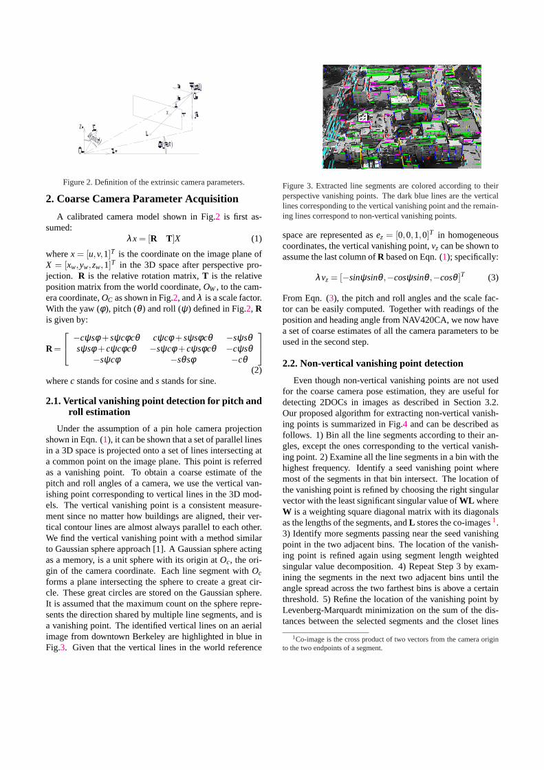
Figure 2.Definition of the extrinsic camera parameters.

2. Coarse Camera Parameter Acquisition

A calibrated camera model shown in Fig.2 is first as-sumed:

λx = [R T]X (1)

wherex = [u,v,1]T is the coordinate on the image plane ofX = [xw,yw,zw,1]T in the 3D space after perspective pro-jection. R is the relative rotation matrix,T is the relativeposition matrix from the world coordinate,OW, to the cam-era coordinate,OC as shown in Fig.2, andλ is a scale factor.With the yaw (φ ), pitch (θ ) and roll (ψ) defined in Fig.2, Ris given by:

R =

−cψsφ +sψcφcθ cψcφ +sψsφcθ −sψsθsψsφ +cψcφcθ −sψcφ +cψsφcθ −cψsθ

−sψcφ −sθsφ −cθ

(2)wherec stands for cosine ands stands for sine.

2.1. Vertical vanishing point detection for pitch androll estimation

Under the assumption of a pin hole camera projectionshown in Eqn. (1), it can be shown that a set of parallel linesin a 3D space is projected onto a set of lines intersecting ata common point on the image plane. This point is referredas a vanishing point. To obtain a coarse estimate of thepitch and roll angles of a camera, we use the vertical van-ishing point corresponding to vertical lines in the 3D mod-els. The vertical vanishing point is a consistent measure-ment since no matter how buildings are aligned, their ver-tical contour lines are almost always parallel to each other.We find the vertical vanishing point with a method similarto Gaussian sphere approach [1]. A Gaussian sphere actingas a memory, is a unit sphere with its origin atOc, the ori-gin of the camera coordinate. Each line segment withOc

forms a plane intersecting the sphere to create a great cir-cle. These great circles are stored on the Gaussian sphere.It is assumed that the maximum count on the sphere repre-sents the direction shared by multiple line segments, and isa vanishing point. The identified vertical lines on an aerialimage from downtown Berkeley are highlighted in blue inFig.3. Given that the vertical lines in the world reference

Figure 3.Extracted line segments are colored according to theirperspective vanishing points. The dark blue lines are the verticallines corresponding to the vertical vanishing point and the remain-ing lines correspond to non-vertical vanishing points.

space are represented asez = [0,0,1,0]T in homogeneouscoordinates, the vertical vanishing point,vz can be shown toassume the last column ofR based on Eqn. (1); specifically:

λvz = [−sinψsinθ ,−cosψsinθ ,−cosθ ]T (3)

From Eqn. (3), the pitch and roll angles and the scale fac-tor can be easily computed. Together with readings of theposition and heading angle from NAV420CA, we now havea set of coarse estimates of all the camera parameters to beused in the second step.

2.2. Non-vertical vanishing point detection

Even though non-vertical vanishing points are not usedfor the coarse camera pose estimation, they are useful fordetecting 2DOCs in images as described in Section 3.2.Our proposed algorithm for extracting non-vertical vanish-ing points is summarized in Fig.4 and can be described asfollows. 1) Bin all the line segments according to their an-gles, except the ones corresponding to the vertical vanish-ing point. 2) Examine all the line segments in a bin with thehighest frequency. Identify a seed vanishing point wheremost of the segments in that bin intersect. The location ofthe vanishing point is refined by choosing the right singularvector with the least significant singular value ofWL whereW is a weighting square diagonal matrix with its diagonalsas the lengths of the segments, andL stores the co-images1.3) Identify more segments passing near the seed vanishingpoint in the two adjacent bins. The location of the vanish-ing point is refined again using segment length weightedsingular value decomposition. 4) Repeat Step 3 by exam-ining the segments in the next two adjacent bins until theangle spread across the two farthest bins is above a certainthreshold. 5) Refine the location of the vanishing point byLevenberg-Marquardt minimization on the sum of the dis-tances between the selected segments and the closet lines

1Co-image is the cross product of two vectors from the camera originto the two endpoints of a segment.

Non-vertical Vanishing Points Detection Algorithm

Enough

segments are

left

No, terminate

Yes

Bin line segments according to their angles

0

-90 45 90 0

10

20

F r e

q u

e n

c y

Choose the bin with maximum frequency. Search for a

seed vanishing point where most of the segments in this

bin intersect. Refine the position of the vanishing point by

segment length weighted singular value decomposition

(SVD) on the stacked segment co-image matrix.

Identify segments crossing the seed vanishing point

from the two adjacent bins and update the location with

SVD again. Iterate this process till the angle spread

among bins is above a certain threshold.

Refine the position of the vanishing point by

Levenberg-Marquardt algorithm.

Eliminate all the identified segments and

record the vanishing point.

-45 Angles (degree)

0

-90 -45 45 90 0

10

20

Angles (degree)

F r e

q u

e n

c y

0

10

20

Angles (degree)

F r e

q u

e n

c y

0 -90 -45 45 90

Figure 4.Non-vertical vanishing point detection algorithm flowchart.

passing through the vanishing point [7]. Remove all the se-lected segments and go back to Step 1 if there are enoughnumber of segments left. The non-vertical vanishing linesobtained using this algorithm for the same sample image areshown in Fig.3.

Since most existing techniques aim to find intersectionsamong as many line segments as possible in an image, theyfail in complex urban settings with many buildings whosealignments are not necessarily parallel [16]. This results inthe intersections in the 3D space to be falsely classified asvanishing points. Our proposed algorithm overcomes thisproblem in several ways. First, we initialize the seed van-ishing point in a bin where all the segments share similarangles. This avoids choosing a seed vanishing point whichis an actual intersection in the 3D space. This preference isalso reinforced by only considering segments whose slopeangle difference is less than the angle spread threshold. Wealso use a segment length weighted singular value decom-position to favor longer segments since they bear less uncer-tainty in their orientation. Finally, since the identified seg-ments are eliminated after each iteration, the convergenceof the algorithm is guaranteed without a priori knowledgeon the number of the vanishing points.

3. Camera parameter refinement

In this section, the set of coarse camera parameters ob-tained in ths first step is refined to achieve sufficient ac-curacy for texture mapping purposes. We employ corre-spondence based on 2DOC features during this process. Inour application, 2DOCs correspond to orthogonal structuralcorners where two orthogonal building contour lines inter-sect. These corners are unique to urban environments, andare limited in number. It might be intuitively appealing touse true 3D corners where three orthogonal lines intersect.However we have empirically found that it is difficult toidentify sufficient number of 3D corners from images giventhe non-ideal line segment extraction. Therefore, we haveopted to relax our constraint of three mutually orthogonalline segments to two. Naturally this leads to many morefalse structural corners extracted from images. In the re-mainder of the paper, we show that these false corners canbe eliminated by feature descriptors, Hough transform andGMSAC. Specifically, we show that the price paid by using2DOC is well compensated by greater number of correctstructural corners from images.

3.1. 2DOC extraction from DSM

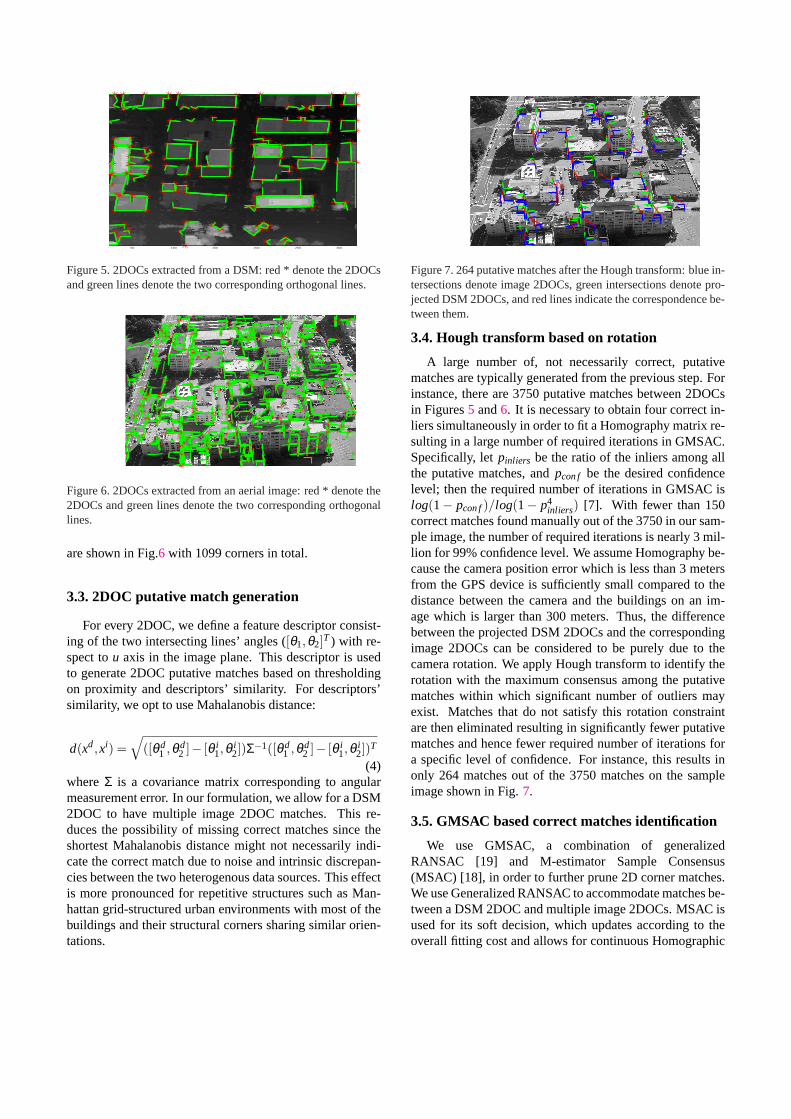
DSM is a depth map representation of a 3D model whichwe assume to have been obtained from LiDAR data. Toextract 2DOCs from DSM, building contours are extractedfrom a DSM with a region growing approach based onthresholding on height differences [5]. Due to the limitedresolution of LiDAR data and inevitable noise, the con-tours tend to be jittery. To straighten jittery edges, we useDouglas-Peucker (DP) line simplification algorithm [3] forits intrinsic ability to preserve the position of 2DOCs sincestructural corners tend to correspond to the extreme verticesin a contour. Once the outer contour of each region is sim-plified, a simple thresholding is performed on the lengths ofthe two intersecting line segments and the intersection an-gle to identify 2DOCs. The 2DOCs are then projected backonto the image plane with the coarse camera parameters inthe first step. The identified 2DOCs from the DSM corre-sponding to the previous sample image are shown on Fig.5with 1548 corners in total.

3.2. 2DOC extraction from aerial images

Since vanishing points represent directions of the corre-sponding groups of line segments in a 3D space, the orthog-onality between each pair of vanishing points also impliesthe orthogonality between the two groups of line segmentseven though they might not appear to be orthogonal in im-ages. The endpoints of line segments belonging to orthogo-nal vanishing point pairs are examined to identify potential2DOC candidates based on proximity. The resulting cor-ners extracted from the sample image using this procedure

50 100 150 200 250 300

Figure 5.2DOCs extracted from a DSM: red * denote the 2DOCsand green lines denote the two corresponding orthogonal lines.

Figure 6.2DOCs extracted from an aerial image: red * denote the2DOCs and green lines denote the two corresponding orthogonallines.

are shown in Fig.6 with 1099 corners in total.

3.3. 2DOC putative match generation

For every 2DOC, we define a feature descriptor consist-ing of the two intersecting lines’ angles ([θ1,θ2]T ) with re-spect tou axis in the image plane. This descriptor is usedto generate 2DOC putative matches based on thresholdingon proximity and descriptors’ similarity. For descriptors’similarity, we opt to use Mahalanobis distance:

d(xd,xi) =√

([θ d1 ,θ d

2 ]− [θ i1,θ

i2])Σ−1([θ d

1 ,θ d2 ]− [θ i

1,θi2])T

(4)whereΣ is a covariance matrix corresponding to angularmeasurement error. In our formulation, we allow for a DSM2DOC to have multiple image 2DOC matches. This re-duces the possibility of missing correct matches since theshortest Mahalanobis distance might not necessarily indi-cate the correct match due to noise and intrinsic discrepan-cies between the two heterogenous data sources. This effectis more pronounced for repetitive structures such as Man-hattan grid-structured urban environments with most of thebuildings and their structural corners sharing similar orien-tations.

Figure 7.264 putative matches after the Hough transform: blue in-tersections denote image 2DOCs, green intersections denote pro-jected DSM 2DOCs, and red lines indicate the correspondence be-tween them.

3.4. Hough transform based on rotation

A large number of, not necessarily correct, putativematches are typically generated from the previous step. Forinstance, there are 3750 putative matches between 2DOCsin Figures5 and6. It is necessary to obtain four correct in-liers simultaneously in order to fit a Homography matrix re-sulting in a large number of required iterations in GMSAC.Specifically, letpinliers be the ratio of the inliers among allthe putative matches, andpcon f be the desired confidencelevel; then the required number of iterations in GMSAC islog(1− pcon f)/log(1− p4

inliers) [7]. With fewer than 150correct matches found manually out of the 3750 in our sam-ple image, the number of required iterations is nearly 3 mil-lion for 99%confidence level. We assume Homography be-cause the camera position error which is less than 3 metersfrom the GPS device is sufficiently small compared to thedistance between the camera and the buildings on an im-age which is larger than 300 meters. Thus, the differencebetween the projected DSM 2DOCs and the correspondingimage 2DOCs can be considered to be purely due to thecamera rotation. We apply Hough transform to identify therotation with the maximum consensus among the putativematches within which significant number of outliers mayexist. Matches that do not satisfy this rotation constraintare then eliminated resulting in significantly fewer putativematches and hence fewer required number of iterations fora specific level of confidence. For instance, this results inonly 264 matches out of the 3750 matches on the sampleimage shown in Fig.7.

3.5. GMSAC based correct matches identification

We use GMSAC, a combination of generalizedRANSAC [19] and M-estimator Sample Consensus(MSAC) [18], in order to further prune 2D corner matches.We use Generalized RANSAC to accommodate matches be-tween a DSM 2DOC and multiple image 2DOCs. MSAC isused for its soft decision, which updates according to theoverall fitting cost and allows for continuous Homographic

Generalized M-estimator Sample Consensus (GMSAC)

Uniformly sample

an image 2D corner

in each group

X d 1

X i a

X d 2

X i b

X d 5

X i g

X d 7

X i z

Uniformly sample 4 groups of

DSM-image 2D corner matches

X d 1

X i a

X i b

X i c

X i d

X d 2

X i a

X i b

X i d

X d 5

X i g

X d 7

X i p

X i z

Fit a Homography matrix from

the four pairs of correspondence

Determine whether there

are three collinear points

Compute the cost of Homography

fitting for all pairs and find inliers

Cost of each pair is

MIN(match error, error threshold)

Below the

currently

optimal cost

No

Yes

Update inliers

percentage and compute

the number of required

iterations

Reach the

number of

required iterations

Yes

No

Terminate

No

Yes

Step 1

Step 2

Step 3

Step 4

Step 5

Step 6

Step 7

Figure 8.Block diagram for GMSAC algorithm.

model improvement. The details of GMSAC are presentedas a block diagram in Fig.8 and can be describes as follows.1) Uniformly sample four groups of DSM-image 2DOCmatches. 2) Inside each group, uniformly sample an im-age 2DOC. 3) Determine whether there are three collinearpoints, a degenerative case for Homography fitting. If so, goto Step 1. Otherwise, move on to Step 4. 4) With four pairsof DSM-image 2DOC matches, a3× 3 Homography ma-trix, H, is fitted with the least squared error [13]. 5) Everypair of DSM-image 2DOC match in every group is then ex-amined with the computed Homography matrix from Step4. Inliers are identified if their squared deviation distancesare below a given error tolerance threshold. The cost as-sociated with each match is the minimum of the squareddeviation distance, and the error tolerance threshold. 6) Ifthe sum of the costs is below the current minimum cost,pinliers is updated and the number of required iterations toachieve the desired confidence level is recomputed. Oth-erwise, another iteration is performed starting from Step 1.7) Terminate the algorithm and output 2DOC match inliersif it has reached the required iteration number. ApplyingGMSAC to our sample image results in 134 matches asshown in Fig.9, which upon manual examination are veri-fied to be correct. Due to the significantly higherpinliers ob-tained from Hough transform in the previous step, we obtainthese 134 matches with fewer than 100 iterations in contrastwith 3 million iterations needed without pruning via Houghtransform.

Finally we apply Lowe’s camera pose recovery algo-rithm [12] to all the identified corner correspondence pairs

Figure 9.134 correct DSM-image matches after GMSAC: blue in-tersections denote image 2DOCs, green intersections denote pro-jected DSM 2DOCs, and red lines indicate the correspondence be-tween them.

from GMSAC to obtain a more accurate set of camera pa-rameters. Texture mapping from images to the 3D model isthen performed according to [4].

4. Results

Our proposed system is tested with 358 aerial imagestaken during a 42-minutes helicopter flight over a 1.3km by2.6km area in the city of Berkeley, California. The coveragearea is divided into three regions with different characteris-tics. The first region is the downtown district, where largebuildings are densely packed among few trees. The sec-ond region is Berkeley campus where large buildings aresparsely distributed among dense trees and vegetation. Therest of the area is grouped as residential where much smallerhouses are densely packed among dense trees.

The correctness of the recovered camera pose is val-idated visually by examining the quality of fit betweenthe projected DSM lines to the building contours in animage. When two sets of lines align sufficiently closeto each other, the recovered pose is deemed to be cor-rect for texture mapping. We have created several tex-tured 3D models using recovered camera poses which havebeen visually validated. Fig.10 shows several screen shotsof such 3D models for downtown, campus and residen-tial models. The resulting textured 3D models can alsobe interactively viewed athttp://www-video.eecs.berkeley.edu/ ∼avz/aironly.htm . Each modelcorresponding to approximately 0.1km2 is textured with 9images for the downtown and campus, and 8 images forthe residential area. The texture alignment in Fig.10 showsthat the poses rated as correct are indeed sufficiently accu-rate to result in visually pleasing texture mapped models.This visual evaluation has been further verified objectivelyby comparing the camera poses with the ones derived frommanual correspondence [2].

In situations where the pose is visually confirmed not tobe sufficiently accurate, we have investigated the source oferror by examining the extracted 2DOCs from both the im-

(a)

(b)

(c)

Figure 10.Screen shots of the texture mapped models from aerialimages with the camera poses estimated using the approach in thispaper: (a)downtown; (b) campus; (c) residential area

age and the DSM. The sources of error can be classifiedinto (a) too few 2DOCs matches and (b) dominant incorrectpose. Clearly, our system has no chance of finding the rightcamera pose when there are too few correct 2DOC matches.This happens when not enough true 2DOCs are extracted ei-ther from the image, or from the DSM, or both. By ”true”2DOCs, we mean those corresponding to actual intersec-tions of two orthogonal building structure lines. Even withsufficient number of correct 2DOC matches, it is possiblethat some combination of 2DOC matches accidentally yielda random camera pose with a small fitting error. This is re-lated to the ill conditioned nature of camera pose recoveryproblem. Both the Hough transform and GMSAC are basedon the assumption that the pose with maximum consensus isthe true camera pose. This assumption tends to break downwhenpinliers is significantly small.

Table1 shows the correct camera pose recovery rate forour proposed approach, for downtown, campus and residen-

Incorrect reasonRegion Correct a b % correct

Downtown 82 0 8 91Campus 57 37 18 51

Residential 78 51 27 50

Total 217 88 53 61

Table 1.Correct pose recovery rate and sources of error in theproposed system for different regions. Incorrect reasona has todo with too few 2DOC matches; incorrect reasonb has to do withdominant incorrect pose.

tial regions. Also shown are the associated reasons for in-correct pose estimates in each region. As seen, our algo-rithm achieves91%correct recovery rate in the downtownregion. In the remaining regions, it faces fundamental dif-ficulties as suggested by the significantly lower recoveryrates. By examining this regional performance difference,a major trade-off on the system performance is revealed.As stated earlier, one reason for camera pose recovery fail-ure is that not enough true 2DOC matches are available.Even though it is possible to extract more 2DOCs by re-laxing certain processing parameters such as minimum linelength threshold, this could potentially lead to additionalfalse 2DOCs, resulting in a decrease inpinliers. This in turnwould result in erroneous pose due to dominant incorrect2DOC matches.

Let us now examine each of the three regions separately.In the downtown region, 2DOCs from both the DSM andthe images are accurately extracted since the line extractionfrom the image and contour simplification from the DSMare both straightforward; furthermore, orthogonal structuralcorners are abundant due to both large and simple rigidbuilding shapes. As such, there are plenty of correct 2DOCmatches. In fact, erroneous camera pose for the 8 imagesin downtown is entirely due to too many incorrect 2DOCmatches, leading to a low percentage of inliers,pinliers.

The analysis on campus and residential areas reveals twofundamental difficulties in extracting true 2DOCs from aDSM. First has to do with the building density in a re-gion. This effect is clearly observed by comparing the re-sults from the downtown and campus areas. Both areas arecharacterized by large buildings; however, the building den-sity is dramatically lower in campus than in downtown. Forinstance, some of the aerial images of the campus only con-tain a portion of a given building since the buildings tendto be larger than the ones in the downtown, and are furtherspread apart. Even if one or two buildings are present in animage, we might not be able to obtain enough 2DOCs dueto imperfect contour simplification and complex buildingstructures on the campus. Furthermore, this small numberof 2DOC matches often does not provide enough constrainton Lowe’s pose recovery algorithm. Since our algorithmrequires a large number of 2DOCs for robustness and accu-

racy, it performs poorly in open fields where buildings aresparsely distributed.

Residential area has a similar building density to down-town. The performance however is much worse due to lackof true 2DOCs from the DSM. This is because the treesnear houses are included as part of buildings after regionsegmentation, and the resulting region contours have manymore sides than the ones from the buildings themselveswithout the trees. It is thus very difficult to extract true2DOCs from these irregular shaped contours. At the sametime, a large number of false 2DOCs have been includedbecause of the trees. This effect is less severe in the campusmodel where the buildings are large enough that relativelysmall distortions on the contour due to tree occlusions canbe removed by DP algorithm.

5. Conclusion and future direction

We have described an algorithm for registering obliqueaerial imagery to 3D geometry model obtained from Li-DAR, and demonstrated its performance over downtown,campus and residential areas of Berkeley using 358 images.Across all three regions, the proposed system achieves61%correct camera pose recovery rate. In particular, its recov-ery rate in downtown district is91%. At the same time, thissystem is computationally efficient. Specifically, the aver-age processing time of 191 seconds per image with IntelXeon 2.8GHz processor is significantly shorter as comparedto over 20 hours of the exhaustive search per image reportedin [4].

Future research should address the low building den-sity and tree occlusion problems. Line matching between aDSM and images can potentially be simple and effective forthe campus region since most of the long line segments arefrom buildings, and occlusion between buildings is insignif-icant. A parameterized roof region fitting could potentiallybe beneficial to both tree removal and 2DOC extraction inthe residential area.

6. Acknowledgement

This research was supported by Army Research Officecontract on Heterogeneous Sensor Webs for Automated Tar-get Recognition and Tracking in Urban Terrain (W911NF-06-1-0076).

References[1] S. Barnard. Interpreting perspective images.Artificial Intel-

ligence, 21:435–462, 1983.[2] M. Ding. Automated texture mapping in a 3d city model.

Master’s thesis, University of California at Berkeley, Dec.2007.

[3] D. H. Douglas and T. K. Peucker. Algorithms for the re-duction of the number of points required to represent a digi-tized line or its caricature.Cartographica: The International

Journal for Geographic Information and Geovisualization,10:112–122, oct 1973.

[4] C. Frueh, R. Sammon, and A. Zakhor. Automated texturemapping of 3d city models with oblique aerial imagery. InInProceedings of the 2nd International Symposium on 3D dataprocessing, visualization and transmission, pages 396–403,Sept. 2004.

[5] C. Fruh and A. Zakhor. Constructing 3d city models bymerging aerial and ground views.IEEE Comput. Graph.Appl., 23(6):52–61, Nov-Dec 2003.

[6] C. Fruh and A. Zakhor. An automated method for large-scale, ground-based city model acquisition.InternationalJournal of Computer Vision, 60(1):5–24, Oct. 2004.

[7] R. I. Hartley and A. Zisserman.Multiple View Geometryin Computer Vision. Cambridge University Press, ISBN:0521540518, second edition, 2004.

[8] S. Hsu, S. Samarasekera, R. Kumar, and H. S. Sawhney. Poseestimation, model refinement and enhanced visualization us-ing video. InCVPR ’00: Proceedings of the 2000 IEEE Com-puter Society Conference on Computer Vision and PatternRecognition, pages 488–495, July 2000.

[9] J. Hu, S. You, and U. Neumann. Automatic pose recovery forhigh-quality textures generation. In18th International Con-ference on Pattern Recognition, pages 561–565, Aug. 2006.

[10] S. C. Lee, S. K. Jung, and R. Nevatia. Automatic integrationof facade textures into 3d building models with a projectivegeometry based line clustering.

[11] L. Liu, I. Stamos, G. Yu, G. Wolberg, and S. Zokai. Mul-tiview geometry for texture mapping 2d images onto 3drange data. InCVPR ’06: Proceedings of the 2006 IEEEComputer Society Conference on Computer Vision and Pat-tern Recognition, pages 2293–2300, Washington, DC, USA,2006. IEEE Computer Society.

[12] D. G. Lowe. Three-dimensional object recognition fromsingle two-dimensional images. Artificial Intelligence,31(3):355–395, 1987.

[13] Y. Ma, S. Soatto, J. Kasecka, and S. S. Sastry.An Invitationto 3-D Vision From Images to Geometric Models. Springer,New York, 2004.

[14] U. Neumann, S. You, J. Hu, B. Jiang, and J. Lee. Augmentedvirtual environments (ave): Dynamic fusion of imagery and3d models. InVR ’03: Proceedings of the IEEE Virtual Real-ity 2003, page 61, Washington, DC, USA, 2003. IEEE Com-puter Society.

[15] J. A. Shufelt. Performance evaluation and analysis of monoc-ular building extraction from aerial imagery.IEEE Trans.Pattern Anal. Machine Intell., 21(4):311–326, 1999.

[16] J. A. Shufelt. Performance evaluation and analysis of van-ishing point detection.IEEE Trans. Pattern Anal. MachineIntell., 21(3):282–288, Mar. 1999.

[17] I. Stamos and P. K. Allen. Geometry and texture recov-ery of scenes of large scale.Comput. Vis. Image Underst.,88(2):94–118, 2002.

[18] P. H. S. Torr and A. Zisserman. Mlesac: a new robust estima-tor with application to estimating image geometry.Comput.Vis. Image Underst., 78(1):138–156, 2000.

[19] W. Zhang and J. Kosecka. Generalized ransac frameworkfor relaxed correspondence problems. InInternational Sym-posium on 3D Data Processing, Visualization and Transmis-sion, 2006.

[20] W. Zhao, D. Nister, and S. Hsu. Alignment of continuousvideo onto 3d point clouds.IEEE Trans. Pattern Anal. Ma-chine Intell., 27(8):1305–1318, 2005.