Embed Size (px)
Citation preview

UNIVERSITAT POLITÈCNICA DE CATALUNYADEPARTAMENT DE LLENGUATGES I SISTEMES INFORMÀTICS
Automatic Pipelining of Elastic Systems
Marc Galceran-Oms
Advisors: Jordi Cortadella and Mike Kishinevsky
June 2011


Preface
The structure of the pipeline is one of the key decisions made during the early design stages of adigital circuit. However, it is often decided based on intuition and the experience of the architects,mainly because of the significant computational costs of design space exploration and the lack ofanalytical optimization methods capable of finding a good pipeline automatically.
This work presents an optimization method that automatically explores microarchitectures inorder to find and evaluate different pipeline options. Exploration is enhanced by the capabilities ofSynchronous Elastic Systems and it is accomplished by applying provably correct-by-constructiontransformations on the microarchitecture. Elastic systems can tolerate latency changes in compu-tations and communications. This elasticity enables new microarchitectural trade-offs aiming ataverage-case optimization (in terms of data variability) rather than worst case.
The first contribution of this work is to present a list of correct-by-construction transforma-tions, such as empty buffer insertion, early evaluation, variable-latency computations or sharingof functional units. These transformations are local, i.e., they are applied to a small part of themicroarchitecture, and it is possible to pipeline a microarchitecture by applying a sequence ofsuch transformations. Some of them can only be applied to elastic systems, since they modify thelatency of the communications and computations.
The second contribution uses the collection of transformations to introduce speculative execu-tion in an elastic system. This solution can be used to implement some well-known architecturalfeatures like branch prediction or error detection and correction schemes.
The third contribution uses elastic transformations to automatically pipeline a microarchitec-tural description of a system or a partially pipelined design. A novel framework for microarchitec-tural exploration is introduced, showing that the optimal pipelining of a circuit can be automaticallyobtained. The optimization is guided by the expected workload of the system.
Finally, a method to analyze the performance of elastic systems and obtain a lower boundof the throughput in presence of early evaluation and variable latency is presented. There werealready existing methods to obtain an upper bound of the throughput using linear programming,but there is no known tractable method to analyze the exact throughput of an elastic system withearly evaluation.
i


Acknowledgments
This thesis would not have been possible without the support of many people.I would like to acknowledge my advisors Jordi Cortadella and Mike Kishinevsky for all the
guidance, support and motivation over the last four years. I am thankful for the opportunities theyhave provided and for all I have learned from them.
During these years, I have had several discussions with people that have helped me to betterunderstand electronic design automation in general and elastic circuits in particular. My gratitudeto Timothy Kam, Alexander Gotmanov, Alexey Pospelov, Satrajit Chatterjee, Dmitry Bufistov,Jorge Júlvez, Josep Carmona, Luciano Lavagno, and also to the Strategic CAD Labs group in IntelCorporation.
I am indebted to Sergi Oliva, Dmitry Bufistov, Nikita Nikitin, Jorge Muñoz, Adrià Gascón,Josep Lluís Berral, Dani Alonso, Miquel Camprodon, Manel Rello and Juan Antonio Farré forcreating a great environment in the office. They have enriched these years with hours of discussionsin topics as diverse as latex and programming tips, research ideas, music, sports, politics, and asoftware to predict soccer results (with little success). I must also thank Ferran Martorell, JonàsCasanova, Juan Antonio Moya, Luca Necchi and Carlos Macián for making the final writing ofthis thesis an exciting period.
This thesis has been supported by a scholarship from Generalitat de Catalunya (FI), by a grantfrom Intel Corporation and the research project FORMALISM CICYT TIN2007-66523.
Finally, thanks to all my family and friends for always being there for me. I also want to expressmy gratefulness to Silvia for all the love, patience and encouragement.
iii


List of Figures
1.1 Synchronous circuit abstraction . . . . . . . . . . . . . . . . . . . . . . . . . . . . 2
1.2 Basic RISC pipeline . . . . . . . . . . . . . . . . . . . . . . . . . . . . . . . . . . 3
1.3 Asynchronous pipeline . . . . . . . . . . . . . . . . . . . . . . . . . . . . . . . . 5
1.4 Synchronous and elastic traces . . . . . . . . . . . . . . . . . . . . . . . . . . . . 7
2.1 Petri net before and after firing transition t. . . . . . . . . . . . . . . . . . . . . . . 15
2.2 Behavior of a design with two internal registers, a and b. At each cycle, a differentvalue is stored at the registers. In the elastic behavior, the symbol ’*’ denotescycles with non-valid data (bubbles). . . . . . . . . . . . . . . . . . . . . . . . . . 20
2.3 The SELF protocol. . . . . . . . . . . . . . . . . . . . . . . . . . . . . . . . . . . 22
2.4 Abstract model for an elastic FIFO. . . . . . . . . . . . . . . . . . . . . . . . . . 23
2.5 Elastic buffer FSM and datapath connection . . . . . . . . . . . . . . . . . . . . . 24
2.6 EB implementation . . . . . . . . . . . . . . . . . . . . . . . . . . . . . . . . . . 25
2.7 Skid-buffer implementation . . . . . . . . . . . . . . . . . . . . . . . . . . . . . . 26
2.8 Join and fork implementations . . . . . . . . . . . . . . . . . . . . . . . . . . . . 27
2.9 Early evaluation firing in transition t, an anti-token is added to the lower inputplace after firing. . . . . . . . . . . . . . . . . . . . . . . . . . . . . . . . . . . . 28
2.10 Elastic channel with dual protocol. Valid+ and Stop+ propagate tokens forward,while Valid− and Stop− propagate anti-tokens backwards. . . . . . . . . . . . . . . 30
2.11 Abstract model for an elastic FIFO with anti-tokens. . . . . . . . . . . . . . . . . . 31
2.12 Linear pipeline with dual elastic buffers. The anti-token flow is stopped at thebeginning of the pipeline by setting S −in to 1. . . . . . . . . . . . . . . . . . . . . . 32
2.13 Dual elastic controllers . . . . . . . . . . . . . . . . . . . . . . . . . . . . . . . . 34
2.14 Example of scheduling of elastic systems . . . . . . . . . . . . . . . . . . . . . . 36
v

2.15 Elastic system with 3 IP blocks that have been elasticized by adding an elasticwrapper around them. The control wires are marked with dotted lines. . . . . . . . 38
2.16 (a) Simple synchronous pipeline, (b) Pipeline after converting flip-flops to EBsusing a pair of latches, the register file is elasticized using a ghost latch, a bubblehas been added after the instruction decoder (c) synchronous elastic system withcontroller; J means join, F fork and EJ early join; EB controllers are marked witha dot if they initially contain a token; paths from control to datapath and fromdatapath to control are dashed, (d) alternative way to elasticize the register file ifthe path from read address to read data is purely combinational. . . . . . . . . . . 41
2.17 (a) Simple elastic pipeline and (b) its elastic marked graph model, each pair ofplaces represent an elastic buffer, the upper place is the forward place and theshadowed lower place is the backward place, which represents available capacity,(c) elastic buffer with joins and forks and (d) its elastic marked graph model, (e)equivalent elastic marked graph with join and fork structure explicitly modeled. . . 42
2.18 TMG model of a synchronous elastic system with two cycles. . . . . . . . . . . . . 44
3.1 Sequence of correct-by-construction transformations applied to a design. . . . . . . 50
3.2 Microarchitectural graphs . . . . . . . . . . . . . . . . . . . . . . . . . . . . . . . 51
3.3 Bypass transformation . . . . . . . . . . . . . . . . . . . . . . . . . . . . . . . . 54
3.4 Retiming transformation . . . . . . . . . . . . . . . . . . . . . . . . . . . . . . . 55
3.5 Example using retiming and recycling . . . . . . . . . . . . . . . . . . . . . . . . 56
3.6 Multiplexor retiming and bubble insertion . . . . . . . . . . . . . . . . . . . . . . 57
3.7 Capacity sizing in a channel. . . . . . . . . . . . . . . . . . . . . . . . . . . . . . 58
3.8 Example of deadlock because of retiming . . . . . . . . . . . . . . . . . . . . . . 59
3.9 Example of retiming and recycling with early evaluation . . . . . . . . . . . . . . 61
3.10 Using little cares to optimize a design . . . . . . . . . . . . . . . . . . . . . . . . 62
3.11 Anti-token transformations . . . . . . . . . . . . . . . . . . . . . . . . . . . . . . 63
3.12 Passive vrs. active anti-tokens . . . . . . . . . . . . . . . . . . . . . . . . . . . . 65
3.13 Sharing transformation . . . . . . . . . . . . . . . . . . . . . . . . . . . . . . . . 68
3.14 (a) Datapath implementation of a shared module, (b) controller of the shared module. 68
3.15 Compositional correctness . . . . . . . . . . . . . . . . . . . . . . . . . . . . . . 70
vi

4.1 Example of speculation in elastic systems: (a) non-speculative system, (b) systemafter bubble insertion, (c) system after Shannon decomposition, (d) final designwith speculation. . . . . . . . . . . . . . . . . . . . . . . . . . . . . . . . . . . . 74
4.2 Example where the outcome of the early-evaluation multiplexor is predicted usingthe proposed method. Each one of the tokens is labeled with a counter (i or i − 1).The stage of EBs after the shared unit has a forward latency of L f and a backwardlatency of Lb. . . . . . . . . . . . . . . . . . . . . . . . . . . . . . . . . . . . . . 77
4.3 . . . . . . . . . . . . . . . . . . . . . . . . . . . . . . . . . . . . . . . . . . . . 78
4.4 (a) Datapath and (b) control for an elastic buffer with no backward latency. . . . . . 79
4.5 Speculation used for error correction and detection . . . . . . . . . . . . . . . . . 81
4.6 Final speculative design corresponding to the original system in Fig. 4.5(a). . . . . 82
4.7 (a) Protocol to synchronize variable-latency units with elastic systems, (b) exampleof a generic variable-latency unit which takes 1 or 2 clock cycles. . . . . . . . . . . 83
4.8 Speculation used for variable latency. . . . . . . . . . . . . . . . . . . . . . . . . 84
5.1 Simple pipelining example . . . . . . . . . . . . . . . . . . . . . . . . . . . . . . 88
5.2 Simulation by case . . . . . . . . . . . . . . . . . . . . . . . . . . . . . . . . . . 90
5.3 Speed-up plot for the introduction example . . . . . . . . . . . . . . . . . . . . . 90
5.4 Pipelining of a simple design with two instructions . . . . . . . . . . . . . . . . . 91
5.5 Another possible pipeline for the graph in Fig. 5.4(a). . . . . . . . . . . . . . . . . 93
5.6 Example with three non-dominated Pareto-point configurations found by retimingand recycling. Their performance metrics are (a) τ = 1,Θ = 0.5, ξ = 2, (b)τ = 2,Θ = 0.66, ξ = 3, (c) τ = 3,Θ = 1, ξ = 3. . . . . . . . . . . . . . . . . . . . . 96
5.7 3 bypasses and retiming using anti-tokens . . . . . . . . . . . . . . . . . . . . . . 96
5.8 Example pipeline with forwarding paths . . . . . . . . . . . . . . . . . . . . . . . 96
5.9 High level view of the exploration algorithm. . . . . . . . . . . . . . . . . . . . . 98
5.10 DLX initial graph. . . . . . . . . . . . . . . . . . . . . . . . . . . . . . . . . . . . 102
5.11 Pipelined DLX graph (F divided into 3 blocks. RF has 3 bypasses and M 9). . . . . 104
5.12 Effective cycle time and area of pipelined designs . . . . . . . . . . . . . . . . . . 105
5.13 Throughput of the memory subsystem given different read latencies and bypassprobability . . . . . . . . . . . . . . . . . . . . . . . . . . . . . . . . . . . . . . . 107
5.14 Ring of pipelines. . . . . . . . . . . . . . . . . . . . . . . . . . . . . . . . . . . . 108
5.15 Effective cycle time for different pipeline depth for γ = 0.1. . . . . . . . . . . . . . 110
vii

5.16 Effective cycle time for different pipeline depths for k = 5. . . . . . . . . . . . . . 1115.17 Flow for video decoding engine design experiment. . . . . . . . . . . . . . . . . . 1135.18 Area-performance trade-off of the original and the optimized decoder. . . . . . . . 114
6.1 TGV example and firing example . . . . . . . . . . . . . . . . . . . . . . . . . . . 1186.2 2-period unfolding example . . . . . . . . . . . . . . . . . . . . . . . . . . . . . . 1216.3 Unfolding example . . . . . . . . . . . . . . . . . . . . . . . . . . . . . . . . . . 1266.4 Portion of an unfolding with reconvergent paths. . . . . . . . . . . . . . . . . . . . 1296.5 Graph representation of an MPEE expression . . . . . . . . . . . . . . . . . . . . 1346.6 Graph representation of correlated expressions . . . . . . . . . . . . . . . . . . . . 1366.7 Throughput of TGV computed using different correlation strategies . . . . . . . . . 1506.8 Run-time of the different performance evaluation versions in seconds for the graphs
in Table 6.3. LB is the presented lower bound method, UB the linear programmingupper bound method, and SIM is the simulation time. The Y-axis is in logscale. . . 154
7.1 Possible implementation for elastic multi-threading support. Grey boxes are sharedunits. . . . . . . . . . . . . . . . . . . . . . . . . . . . . . . . . . . . . . . . . . . 165
viii

List of Tables
4.1 Example trace from Fig. 4.1(d) . . . . . . . . . . . . . . . . . . . . . . . . . . . . 76
5.1 Delay and area numbers for DLX example using NAND2 with FO3 as unit delayand unit area. . . . . . . . . . . . . . . . . . . . . . . . . . . . . . . . . . . . . . 103
5.2 Parameter ranges in the experiments. . . . . . . . . . . . . . . . . . . . . . . . . . 1095.3 Number of bypasses performed in the pipelined design. . . . . . . . . . . . . . . . 1115.4 Run-time of the whole exploration method (including simulations) for different
number of pipelines (k) and different depth ranges (D) in seconds. The minimum,maximum, mean, medium and quartiles are shown for each range. . . . . . . . . . 112
6.1 Experimental results on random graphs with early-evaluation nodes and no variable-latency units . . . . . . . . . . . . . . . . . . . . . . . . . . . . . . . . . . . . . . 151
6.2 Experimental results on random graphs with variable-latency units and no early-evaluation nodes . . . . . . . . . . . . . . . . . . . . . . . . . . . . . . . . . . . . 152
6.3 Experimental results on random graphs with early-evaluation nodes and variable-latency units . . . . . . . . . . . . . . . . . . . . . . . . . . . . . . . . . . . . . . 153
6.4 Configurations found by the retiming and recycling method on graph G8. Thefirst column shows the throughput found by simulation and the order according tothis throughput. The second column shows the throughput found by the presentedlower bound method and the corresponding order. Finally, the third column showsthe throughput according to the upper bound method and the corresponding order. . 155
6.5 Number of swaps needed to produce a correct order. Confs shows how manyRR configurations where created, LB and UB swaps show how many swaps wereneeded to achieve the correct configuration order, and “swap diff” shows the aver-age throughput difference for the swapped configurations. . . . . . . . . . . . . . . 156
ix

x

List of Algorithms
1 Bypass_One(G), exploration by adding one bypass at a time . . . . . . . . . . . . . 1002 Bypass_All(G), pipelining by adding one bypass per memory element at a time . . . 1013 Top-level Exploration Algorithm. . . . . . . . . . . . . . . . . . . . . . . . . . . . 1014 Overview of the top level algorithm. . . . . . . . . . . . . . . . . . . . . . . . . . . 1215 BuildMPEE, construct an MPEE expression from an unfolding. . . . . . . . . . . . 1336 EvaluateRecursive, algorithm that evaluates an MPEE expression. . . . . . . . . . . 1387 A_exact, algorithm that evaluates an MPEE expression. . . . . . . . . . . . . . . . 1398 EvaluateUB, algorithm that computes an upper bound of the result of evaluating an
MPEE expression. . . . . . . . . . . . . . . . . . . . . . . . . . . . . . . . . . . . 1419 A_prune, algorithm that computes an upper bound of all firing times by ignoring all
correlations during evaluation. . . . . . . . . . . . . . . . . . . . . . . . . . . . . . 141
xi


Contents
1 Introduction 11.1 Synchronous Circuits . . . . . . . . . . . . . . . . . . . . . . . . . . . . . . . . . 2
1.2 Pipelining . . . . . . . . . . . . . . . . . . . . . . . . . . . . . . . . . . . . . . . 3
1.3 Elasticity . . . . . . . . . . . . . . . . . . . . . . . . . . . . . . . . . . . . . . . 4
1.4 Why Synchronous Elastic Systems? . . . . . . . . . . . . . . . . . . . . . . . . . 8
1.5 Overview of the Contributions . . . . . . . . . . . . . . . . . . . . . . . . . . . . 10
1.6 Organization of the Thesis . . . . . . . . . . . . . . . . . . . . . . . . . . . . . . 13
2 State of the Art 152.1 Preliminaries . . . . . . . . . . . . . . . . . . . . . . . . . . . . . . . . . . . . . 15
2.1.1 Petri Nets . . . . . . . . . . . . . . . . . . . . . . . . . . . . . . . . . . . 15
2.1.2 Marked Graphs . . . . . . . . . . . . . . . . . . . . . . . . . . . . . . . . 16
2.1.3 Throughput of a TMG . . . . . . . . . . . . . . . . . . . . . . . . . . . . 17
2.1.4 Linear Programming . . . . . . . . . . . . . . . . . . . . . . . . . . . . . 17
2.2 Synchronous Elastic Systems . . . . . . . . . . . . . . . . . . . . . . . . . . . . . 18
2.2.1 Definitions . . . . . . . . . . . . . . . . . . . . . . . . . . . . . . . . . . 18
2.2.2 SELF Protocol . . . . . . . . . . . . . . . . . . . . . . . . . . . . . . . . 21
2.2.3 Early Evaluation and Token Counterflow . . . . . . . . . . . . . . . . . . 28
2.2.4 Verification . . . . . . . . . . . . . . . . . . . . . . . . . . . . . . . . . . 35
2.2.5 Scheduling . . . . . . . . . . . . . . . . . . . . . . . . . . . . . . . . . . 37
2.2.6 Granularity of elastic islands . . . . . . . . . . . . . . . . . . . . . . . . . 37
2.2.7 Synthesis Flow . . . . . . . . . . . . . . . . . . . . . . . . . . . . . . . . 39
2.2.8 Modeling Elastic Systems with Marked Graphs . . . . . . . . . . . . . . . 41
2.2.9 Performance Analysis of Elastic Systems . . . . . . . . . . . . . . . . . . 43
xiii

2.3 Automatic Pipelining . . . . . . . . . . . . . . . . . . . . . . . . . . . . . . . . . 46
2.4 Conclusions . . . . . . . . . . . . . . . . . . . . . . . . . . . . . . . . . . . . . . 47
3 Correct-by-construction Transformations 493.1 Introduction . . . . . . . . . . . . . . . . . . . . . . . . . . . . . . . . . . . . . . 49
3.2 Microarchitectural graphs . . . . . . . . . . . . . . . . . . . . . . . . . . . . . . . 51
3.3 Toolkit . . . . . . . . . . . . . . . . . . . . . . . . . . . . . . . . . . . . . . . . . 53
3.4 Latency-Preserving Transformations . . . . . . . . . . . . . . . . . . . . . . . . . 54
3.4.1 Bypass . . . . . . . . . . . . . . . . . . . . . . . . . . . . . . . . . . . . 54
3.4.2 Retiming . . . . . . . . . . . . . . . . . . . . . . . . . . . . . . . . . . . 56
3.4.3 Multiplexor Retiming . . . . . . . . . . . . . . . . . . . . . . . . . . . . . 57
3.5 Recycling . . . . . . . . . . . . . . . . . . . . . . . . . . . . . . . . . . . . . . . 57
3.6 Buffer Capacities . . . . . . . . . . . . . . . . . . . . . . . . . . . . . . . . . . . 58
3.7 Early Evaluation . . . . . . . . . . . . . . . . . . . . . . . . . . . . . . . . . . . 60
3.7.1 Critical Cores and Little Cares . . . . . . . . . . . . . . . . . . . . . . . . 61
3.8 Anti-token Insertion . . . . . . . . . . . . . . . . . . . . . . . . . . . . . . . . . . 63
3.8.1 Passive or Active Anti-tokens . . . . . . . . . . . . . . . . . . . . . . . . 64
3.9 Variable-latency Units . . . . . . . . . . . . . . . . . . . . . . . . . . . . . . . . 66
3.10 Sharing of Functional Units . . . . . . . . . . . . . . . . . . . . . . . . . . . . . . 67
3.11 Verification . . . . . . . . . . . . . . . . . . . . . . . . . . . . . . . . . . . . . . 69
3.12 Conclusion . . . . . . . . . . . . . . . . . . . . . . . . . . . . . . . . . . . . . . 71
4 Speculation 734.1 Introduction . . . . . . . . . . . . . . . . . . . . . . . . . . . . . . . . . . . . . . 74
4.2 Speculative Execution . . . . . . . . . . . . . . . . . . . . . . . . . . . . . . . . . 75
4.3 EBs with Zero Backward Latency . . . . . . . . . . . . . . . . . . . . . . . . . . 78
4.4 Design Examples . . . . . . . . . . . . . . . . . . . . . . . . . . . . . . . . . . . 80
4.4.1 Resilient Designs . . . . . . . . . . . . . . . . . . . . . . . . . . . . . . . 80
4.4.2 Variable-Latency Unit . . . . . . . . . . . . . . . . . . . . . . . . . . . . 82
4.5 Conclusion . . . . . . . . . . . . . . . . . . . . . . . . . . . . . . . . . . . . . . 84
5 Automatic Pipelining 875.1 Introduction . . . . . . . . . . . . . . . . . . . . . . . . . . . . . . . . . . . . . . 88
5.2 Correct-by-construction Pipelining of a Simple Example . . . . . . . . . . . . . . 89
xiv

5.3 Exploration Engine . . . . . . . . . . . . . . . . . . . . . . . . . . . . . . . . . . 92
5.3.1 Retiming and Recycling . . . . . . . . . . . . . . . . . . . . . . . . . . . 94
5.3.2 Bypassing and Forwarding . . . . . . . . . . . . . . . . . . . . . . . . . . 95
5.3.3 Two-phase Exploration . . . . . . . . . . . . . . . . . . . . . . . . . . . . 98
5.3.4 Exploration Algorithm . . . . . . . . . . . . . . . . . . . . . . . . . . . . 99
5.4 Pipelining Examples . . . . . . . . . . . . . . . . . . . . . . . . . . . . . . . . . 102
5.4.1 DLX pipeline . . . . . . . . . . . . . . . . . . . . . . . . . . . . . . . . . 103
5.4.2 Ring of pipelines . . . . . . . . . . . . . . . . . . . . . . . . . . . . . . . 108
5.5 Video Decoding Engine . . . . . . . . . . . . . . . . . . . . . . . . . . . . . . . . 113
5.6 Conclusion . . . . . . . . . . . . . . . . . . . . . . . . . . . . . . . . . . . . . . 115
6 Symbolic Performance Analysis 1176.1 Introduction . . . . . . . . . . . . . . . . . . . . . . . . . . . . . . . . . . . . . . 117
6.2 Problem Formulation . . . . . . . . . . . . . . . . . . . . . . . . . . . . . . . . . 123
6.2.1 Multi-guarded Marked Graph . . . . . . . . . . . . . . . . . . . . . . . . 123
6.2.2 Unfoldings . . . . . . . . . . . . . . . . . . . . . . . . . . . . . . . . . . 126
6.2.3 Single-Server Semantics . . . . . . . . . . . . . . . . . . . . . . . . . . . 127
6.2.4 Throughput . . . . . . . . . . . . . . . . . . . . . . . . . . . . . . . . . . 127
6.2.5 Timing Simulation of a TGV . . . . . . . . . . . . . . . . . . . . . . . . . 128
6.3 Max-plus Algebra with Early Evaluation . . . . . . . . . . . . . . . . . . . . . . . 129
6.3.1 Definitions . . . . . . . . . . . . . . . . . . . . . . . . . . . . . . . . . . 130
6.3.2 Representation of MPEE Expressions . . . . . . . . . . . . . . . . . . . . 132
6.3.3 Lower and Upper Bounds of Expressions . . . . . . . . . . . . . . . . . . 135
6.3.4 Exact Evaluation of MPEE Expressions . . . . . . . . . . . . . . . . . . . 135
6.3.5 Upper Bound Evaluation of MPEE Expressions . . . . . . . . . . . . . . 139
6.3.6 Algorithm Complexity . . . . . . . . . . . . . . . . . . . . . . . . . . . . 145
6.4 Number of Periods of the Unfolding . . . . . . . . . . . . . . . . . . . . . . . . . 146
6.4.1 Convergence of A_exact . . . . . . . . . . . . . . . . . . . . . . . . . . . 146
6.4.2 Convergence of the Upper Bound Method, A_prune . . . . . . . . . . . . 148
6.4.3 Example . . . . . . . . . . . . . . . . . . . . . . . . . . . . . . . . . . . 149
6.5 Experimental Results . . . . . . . . . . . . . . . . . . . . . . . . . . . . . . . . . 151
6.5.1 Random Graphs . . . . . . . . . . . . . . . . . . . . . . . . . . . . . . . 151
6.5.2 Evaluating Relative Performance . . . . . . . . . . . . . . . . . . . . . . . 153
xv

6.6 MPEE Simplification using SMT . . . . . . . . . . . . . . . . . . . . . . . . . . . 1556.7 Conclusion . . . . . . . . . . . . . . . . . . . . . . . . . . . . . . . . . . . . . . 157
7 Conclusions 1617.1 Contributions . . . . . . . . . . . . . . . . . . . . . . . . . . . . . . . . . . . . . 1617.2 Further Research . . . . . . . . . . . . . . . . . . . . . . . . . . . . . . . . . . . 163
xvi

Chapter 1
Introduction
CMOS process scaling, predicted by Moore’s Law [114], enabled a steady increase in the complex-ity and the operating frequencies of integrated circuits. While the race on the operating frequencieshas come to an end, technology shrinking continues, providing integration capacity of billions oftransistors. The evolution of technologies enables the integration of complex systems in a singlechip (System-on-Chip, SoC), and it has brought the popularization of multi-cores [18,84,124,145].
As designs have become more and more complex, Electronic Design Automation (EDA, akaComputed Aided Design, CAD) has rapidly increased in importance. During the early years of thesemiconductor industry, integrated circuits were designed by hand and the layout was also builtmanually. Incrementally, more and more stages of design were performed in an automatic or semi-automatic way. Place and route tools appeared, hardware description languages, verification tools,simulation tools, logic synthesis, etcetera. Today, EDA is present in all stages needed to build anintegrated a circuit: design (from high level synthesis to physical synthesis), simulation, analysis,verification and manufacturing.
However, since technologies continue to shrink, the known problems become more challengingand new problems emerge. While synchronous circuits have been the dominant paradigm forcircuit design through all these years, the asynchronous alternative has always been there claimingto provide a possible solution for the dark clouds that hover over the synchronous world.
Synchronous elastic systems have emerged in the last years as a middle ground solution be-tween synchronous and asynchronous circuits. They can be designed and implemented usingregular synchronous flows and tools, but they provide some of the advantages of asynchronousdesigns since they can tolerate variations in the latencies of the computations and the communica-
1

2 1.1. SYNCHRONOUS CIRCUITS
combinationallogic
sequentialelements
clock inputs
outputs
(a)
clock
......
(b)
Figure 1.1: (a) Abstraction of a synchronous circuit, (b) Synchronous pipeline.
tions.
This tolerance can be used to separate performance critical parts from non-critical and op-timize the former ones in isolation, while non-critical parts are removed from critical paths byadding latency to their computations. This is an example of the optimization opportunities that areenabled by elasticity. This thesis proposes a framework to leverage synchronous elastic systems inorder to perform design space exploration of microarchitectures automatically. This chapter putssynchronous elastic systems into context and motivates the contributions of this thesis.
1.1 Synchronous Circuits
Figure 1.1(a) shows a very common abstraction for synchronous circuits. A synchronous circuitis formed by sequential elements (aka state signals), which are synchronized by an external clock,and the combinational logic, which performs the actual computation. The sequential elements loada new stable state each time a clock edge is delivered. The clock signal provides a time referenceto the circuit.
Between two consecutive edges of the clock, the combinational elements compute the nextstable state. Signals need some time to settle to their new state before a new clock edge can arrive.Otherwise, the results can be incorrect. The minimum time distance between two consecutiveclock edges is the cycle time of the design, and it determines the maximum clock frequency atwhich the circuit can run. The slowest timing path determines the cycle time, and it is known asthe critical path of the design.
The division of the computation in cycles delimited by a clock is very simple and intuitive.Furthermore, the separation between sequential elements that store the state and combinationalelements that perform computations makes it easy to reason about synchronous systems. Thissimplicity is reflected in design, synthesis, timing analysis, testing and verification. Furthermore,most EDA tools target explicitly synchronous systems and most designers are only trained to use

CHAPTER 1. INTRODUCTION 3
Instr No. Pipeline Stage1 IF ID EX MEM WB2 IF ID EX MEM WB3 IF ID EX MEM WB4 IF ID EX MEM5 IF ID EX
Cycle 1 2 3 4 5 6 7
Figure 1.2: Basic RISC pipeline (IF = Instruction Fetch, ID = Instruction Decode, EX = Execute,MEM = Memory access, WB = Register write back).
them. Thus, the vast majority of circuits designed by the industry nowadays follow the synchronousparadigm.
1.2 Pipelining
In order to increase the throughput of a circuit, digital systems can be divided in stages con-nected forming a pipeline allowing the concurrent execution of multiple instructions or computa-tions [140], as shown in Fig. 1.1(b). Each stage of the pipeline works on a part of an instructionwhile other stages work on other instructions in parallel. Each instruction enters at one end, pro-gresses through the stages, and exits at the other end. Pipelining is a key implementation techniquefor the design of efficient circuits.
A pipeline is like an assembly line. Every step of an automobile assembly line works in parallelwith the other steps, although on a different car. In a computer pipeline, each step (or stage) ofthe pipeline performs a different part of the computation. This way, the system clock can havea smaller cycle time, since the combinational logic between stages execute simpler computationscompared to completing the whole computation in just one clock cycle, and hence it can run faster.
As an example, a basic RISC pipeline [75] typically has 5 stages, Instruction Fetch, Instruction
Decode, Execute, Memory access and Write Back. Figure 1.2 shows an example execution forthis basic pipeline. The first instruction is fetched on the first clock cycle. On the second one, thefirst instruction is decoded while the second one enters the pipeline and is fetched, and so on. Onthe sixth clock cycle, the first instruction has already been completed, and the second to the fifthinstructions are being executed.
Ideally, the speed-up of a pipeline with 5 stages should be 5X, compared to the same un-

4 1.3. ELASTICITY
pipelined system. The same computation that had to be accomplished within one clock cycle cannow be evenly divided in 5 parts, and hence each stage only needs 20% of the original cycle time.However, the ideal speed-up is typically not possible when the pipeline is deep enough. First,because it can be difficult to evenly balance the combinational logic among the stages, second, be-cause of the overhead (setup time and clock skew) of the additional registers, and most important,because there may be dependencies between consecutive or close instructions.
While assembly code assumes that instructions are executed sequentially, pipelining invalidatesthis assumption. Data hazards appear when an instruction depends on the results of previous ones.These data dependencies can be solved by different techniques, such as forwarding and stalling. Ifthe pipeline must be stalled, it is not possible to complete one instruction per cycle anymore. Forexample, consider the following instructions:
add $R2, $R1, 1add $R4, $R2, $R3
The processor will add 1 to the contents of register R1 and store it in R2. Then, the execution ofthe second instruction will read registers R2 and R3, add their values and store the result in R4. In apipeline, the first instruction will be just one stage ahead of the second, so R2 is not updated whenthe second instruction wants to read it. A way to solve this hazard is to stall the second instructionuntil the first one has completed. A second solution is to forward the result of the first instructionto the second one as soon as it is available, even if the first instruction has not completely finished.For example, an extra path can be added from the stage Execute to the stage Decode so that theresult of the first instruction can be sent to the second one as soon as Execute knows the result forinstruction add, avoiding stages MEM and WB.
In a microprocessor, the performance of a pipeline can be measured in instructions per cycle(IPC), i.e., the number of instructions completed on average per clock cycle. The inverse of theIPC, the CPI, or how many clock cycles are needed on average to complete an instruction, is alsoused. Finally, the average time per instruction can be found by multiplying the CPI by the cycletime of the circuit.
1.3 Elasticity
Since the early days of EDA, designers have been using optimization tools to improve the qualityof the circuits (area, delay or power). For example, the techniques for two-level and multi-level

CHAPTER 1. INTRODUCTION 5
...
control control controlreq/validack/stop ...
...
...Figure 1.3: Asynchronous pipeline, each register is controlled by a local control which synchro-nizes with its neighbors.
combinational logic synthesis exploit the properties of Boolean algebra to transform gate netlistswithin the boundaries of the sequential elements of the circuit [58, 71]. With this approach, thebehavior of the primary outputs and state signals is preserved, whereas the combinational parts areoptimized.
A new generation of techniques enabled the crossing of the sequential boundaries and intro-duced new optimizations that can change the behavior of the state signals while preserving thebehavior at the primary outputs. This field is known as sequential logic synthesis and includestransformations such as state encoding [8], redundant latch removal [14], retiming [98] and by-passing of memory elements [16].
All the previous transformations still preserve a cycle-accurate behavioral equivalence of thesystem: what is observable at the outputs of the system at the i-th clock cycle is independent fromthe optimizations performed on the system.
Maintaining the cycle accuracy imposes severe constraints on the type of optimizations that canbe used in a circuit. For example, changing the structure of a pipeline or modifying the latency ofa functional unit may not be applicable unless the global architecture of the system is transformedand adapted to the new timing requirements. This limitation is unacceptable for large systems thatmay be susceptible to late-stage re-design decisions to meet the timing specifications.
Elasticity has emerged as a new paradigm to overcome these limitations, enabling the designof systems that are tolerant to the dynamic changes of the computation and communication delays.The concept of elasticity has been widely used in asynchronous circuits. For example, the termMicropipeline was proposed by Sutherland [149] to denote event-driven elastic pipelines.
In contrast to synchronous circuits, asynchronous circuits are not governed by an external clocksignal. Instead, each of its components is autonomous and it communicates with its neighbors inorder to synchronize data flow, as shown in Fig. 1.3. This way delay variability can be tolera-ted. Typically, synchronization is performed by a handshake protocol where the sender indicates

6 1.3. ELASTICITY
whether it is ready to transmit new data and the receiver indicates whether it is ready. Thesehandshake signals are often called request and acknowledge.
Different classes of asynchronous designs offer different advantages compared to synchronousdesigns. Asynchronous designs have the potential to provide low power consumption, becausetransistors only switch when a useful computation is performed. Asynchronous designs also havebetter modularity and composability, because timing constraints are more flexible and independentfrom module to module. In synchronous designs, it must be ensured that the circuit will meet thetiming even in the worst-case conditions. Hence, the clock frequency is determined by the worstcase. However, in asynchronous designs, the circuit speed adapts to the temperature and voltageconditions. This way, variability can be better tolerated. Furthermore, if the circuit is not operatingunder the worst-case conditions, the circuit can consume less power (or it can run faster).
Although it has various advantages, a very small part of the circuits are actually designedusing this paradigm. One of the big disadvantages of asynchronous designs is that they typicallyrequire a completely different design flow. The tools to handle asynchronous circuits are lessmature and most designers have more experience and expertise on designing synchronous circuits.Furthermore, the performance of the circuit is no longer determined by a fixed clock frequency,and it becomes more difficult to analyze what the actual performance is. There is an area overheadcompared to synchronous designs because the handshake signals must be placed and routed alongwith the design. Finally, verification and testing of asynchronous designs is more challenging.
Elasticity can be discretized so that it can be implemented within a synchronous system, be-coming a Latency Insensitive System [31, 32]. The handshake signals are then synchronized withthe main clock of the system, i.e., each of the controllers shown in Fig. 1.3 implements a syn-chronous protocol instead of an asynchronous one. Many of the properties and optimization tech-niques of asynchronous designs are also applicable to latency-insensitive designs. In this context,the pair of handshake signals are typically called valid and stop, indicating respectively the validityof the data in the communication channel and the availability of the receiver to store the incomingdata during each clock cycle. Different variants of synchronous elasticity have been proposed inthe literature [53, 82, 127, 152].
The handshake controllers of elastic systems govern the flow of data along the datapath. Insteadof implementing a monolithic stall controller that often resides on a critical path, the control is fullydistributed alongside the datapath. Furthermore, each handshake controller produces a clock forthe part of the datapath it manages. This way, each clock network is independent and becomessimpler to design.

CHAPTER 1. INTRODUCTION 7
8 6 2 4+7
1 4 0 1
2 2 3
time
(a)
1
2 37
1 0
2
4
426+ 8
(b)
1
2 37
1 0
2
4426+ 8
(c)
Figure 1.4: (a) Synchronous adder, (b) elastic adder, (c) synchronous elastic adder, shaded boxesrepresent idle cycles.
Latency-insensitive designs can tolerate any modification in the communication and computa-tion latency. Thus, the functionality of the system only depends on the functionality of its com-ponents and not on their timing characteristics. The goal of this methodology is to guarantee thatcorrect modules composed in a latency-insensitive framework will behave correctly.
Figure 1.4(a) shows an example of a conventional synchronous circuit performing additions.Each clock cycle, the circuit receives new inputs and produces the corresponding outputs. Theenvironment is designed under the assumption that all operations will take one cycle.
With elasticity, the concept of behavioral equivalence is relaxed in a way that no cycle accuracyis required. Instead, the sequence of valid data is observed and preserved, as if one would connectFIFOs with non-deterministic delays at the inputs and outputs of the system. Figure 1.4(b) showsan example of an elastic system in an asynchronous environment, representing the same circuit.Inputs can arrive at any time. There is an underlying control that synchronizes them, the input thatarrives earlier waits for the latest one. Once both inputs are available, the adder can produce a newoutput and send an acknowledge to the inputs so that they know they can send the next data item.
Figure 1.4(c) shows a synchronous elastic version of the same circuit, in which the empty cellsrepresent non-valid data. In contrast to Fig. 1.4(b), time is discretized, and if data items are notavailable during one clock cycle, the module waits for the next clock cycle. It can be observed

8 1.4. WHY SYNCHRONOUS ELASTIC SYSTEMS?
that the traces of valid data for each signal are the same as in the non-elastic circuit. Although thetiming is elastic, the causality relations between data items is preserved, e.g., the value a + b isalways generated after having received the corresponding values of a and b.
The main metric to measure the performance of an elastic system can still be the average timeper instruction, as in a synchronous pipeline. In asynchronous systems the concept of cycle timeis different because there is no clock. Thus, the time per instruction cannot be found just bymultiplying the CPI by the cycle time, it is necessary to analyze how often actual computationoccurs. Similarly, in synchronous elastic systems, the rate of cycles with valid computation mustalso be evaluated in order to determine the actual performance of the system.
1.4 Why Synchronous Elastic Systems?
Latency Insensitive (or synchronous elastic) systems offer some of the advantages of asynchronoussystems, while they can be designed using synchronous CAD flows and tools. Elasticity may helpsolve or alleviate some of the current problems of circuit design. Let us review some of them andhow elasticity may be a resource to mitigate these problems.
At the early 90s, the performance of a processor was considered to be determined by its clockrate. The advances in manufacturing, which allowed to double the number of transistors appro-ximately every 18 months, allowed the frequency to double as well. The scaling of the clockfrequencies was achieved by building deeper pipelines, providing more parallelism and hence abetter IPC. Furthermore, a set of architectural techniques to reduce the stalls in the pipeline wereintroduced, such as out-of-order execution, threading, duplication of functional units and specula-tive execution.
By the mid 2000s, however, frequency scaling could not be sustained anymore. The improve-ment in frequency did not provide the same improvement in the actual performance of the cir-cuit [3]: the level of parallelism could not be further improved within a single pipeline. Further-more, supply voltage did not decrease at the same pace [129], and the power consumption roseconsiderably. Although there are some fundamental barriers [17], technology scaling still goes onnowadays. The extra space achieved by technology scaling is used to increase the performanceof the circuits by adding more cores in a single chip working in parallel, going into Systems onChip (SoC) and high-end chip multi-processors (CMPs). Besides, chips for mobile devices haveemerged in the market. Such designs have tight power budgets in order to increase battery run-time.Thus, power has become an important design constraint in some circuits.

CHAPTER 1. INTRODUCTION 9
Elasticity can help to improve the overall performance of a design because it allows a designerto separate the performance critical parts from the non-critical ones. Then, the critical parts can beoptimized in isolation, increasing their parallelism or using some techniques available for elasticsystems, such as variable-latency units (e.g. using telescopic units [11], which can be naturallyintegrated into an elastic system). On the other hand, non-critical parts can have a relaxed timingand a long latency, reducing power consumption without a big impact on the overall performance.Furthermore, power consumption may also be reduced because the distributed localized control ofelastic systems avoids unnecessary communications and computations.
Variability is one of the aspects with increasing importance in chip design [13, 117]. Thereexists variability among different chips of the same design (inter-die variability) due to imperfec-tions in the manufacturing technology. As wires and transistors become smaller and smaller, thedifference in the speed of the circuit due to these imperfections grows larger. Furthermore, thereis also variability within a single chip (within-die variability). Different parts of the chip may beworking at different operating conditions (e.g., at different temperatures), and hence, they have adifferent timing. Unpredictable delays compel designers to use conservative margins that cannotbe adjusted in order to achieve the full potential of current process technologies.
Elasticity can tolerate timing variations in the computations and communications of a circuitand its environment, even if these variations are unpredictable. This tolerance may be used to adaptthe voltage and speed of the circuit to the operating conditions without affecting the correctness ofthe computations. The intrinsic modularity of elastic systems also guarantees that changes in thespeed of one module do not affect the correctness of the inter-module interaction.
The impact of wire delay on design performance has been growing on deep submicron design,due to the mismatch in scaling trends of gate delays and interconnect delays over process gen-erations [3, 47]. The maximum distance a signal can travel along an interconnect within a clockcycle gradually decreases as the process technology scales down [138]. Traditional design methodsrequire knowing communication delays in advance, but the distance between two locations, andhence the wire delay, cannot be accurately estimated on early design stages because the floor-planis not available.
Elasticity can help to cope with long communications because it is possible to insert emptysequential elements, or bubbles, without affecting the correctness of the design. Hence, they canbe added at any design stage to cut a long wire. While bubbles can solve timing problems dueto long wires, they can also decrease the overall throughput of the system, since communicationswill have a larger latency. Hence, they must be added carefully to avoid a dramatic performance

10 1.5. OVERVIEW OF THE CONTRIBUTIONS
penalty.Current chips have the capacity to contain billions of transistors, but there is a gap between
such manufacturing capabilities and the ability of designers to quickly put together a complexdevice. Reuse of existing intellectual property (IP) can help closing this gap and meeting tighttime to marked constraints. As the number of IP elements on a single chip increases and the SoCmarket becomes more important, methods that allow faster design and re-usability of IP elementsare needed.
Elastic systems can also help reusing and integrating IP blocks, since they define a simple com-munication protocol which can be used for synchronization and data transfer of already existingblocks. The functionality of elastic systems does not depend on the timing of its modules, onlyon the order of the transmitted data. Thus, it becomes easier to integrate modules with differenttiming. Since elastic controllers are distributed and there are no global signals to broadcast, thisparadigm scales well to a large number of integrated IP blocks.
1.5 Overview of the Contributions
Elasticity opens the door to a new avenue of correct-by-construction behavior-preserving trans-formations for optimizing systems that cannot be systematically applied in a non-elastic context.These transformations take advantage of the tolerance of elastic systems to latency changes, andthe fact that stalls and data synchronization is handled inherently by elastic controllers. The inser-tion of “empty” sequential elements in a pipeline, the execution of variable-latency computations,the addition of bypass circuits with early-evaluation firing semantics or the speculative executionof operations are some of the transformations that can be considered to increase the performanceof a circuit.
The main objective of this thesis is to leverage these transformations in order to provide anoptimization framework for elastic circuits. The contributions of this thesis are the following:
1. A collection of correct-by-construction transformations applicable to elastic systems.Some of these transformations can be applied to conventional synchronous systems, and theyhave been adapted to elastic systems. The rest of the transformations can only be applied inan elastic environment because they modify the latency of the system. This collection is thestarting point of the optimization framework proposed in this thesis.
It is verified that each of the transforms does not change the functionality of the design. The

CHAPTER 1. INTRODUCTION 11
timing of the events may change, but their order and their correct synchronization is alwayspreserved.
All of these transformations can be applied to asynchronous circuits as well, but this the-sis focuses on synchronous elastic systems, since verification and synthesis tools are betterprepared to handle synchronous circuits and it is more practical to work with them.
2. A method to introduce speculative execution in elastic systems. This contribution showshow speculation can be inserted in an elastic system by applying a sequence of correct-by-construction transformations from the available collection of transforms. Speculation is awidely-used technique that increases the parallelism of a design by starting computationsthat are likely to be useful before it is known whether they will be needed.
When speculating on a choice in an elastic system, one of the possible outcomes is predicted,based on some knowledge of the system, and the other possible choices are stalled. Suchstalling is handled naturally by the handshake controllers of elastic systems. Then, normalcomputation continues with the predicted choice.
Once the outcome of the prediction is known, the stalled data values can be discarded ifthe prediction was right, or used if the prediction failed. On mispredictions, the speculativeexecution is canceled. Assuming most of the times the predictions are successful, correctioncomputations will be rarely needed, and the overall performance of the system will be bettercompared to a non-speculative execution.
Several applications of this method are shown, such as branch prediction, error detection andcorrection units and an efficient implementation of variable-latency units.
3. Automatic correct-by-construction pipelining. One of the significant choices made dur-ing the early design stages is the structure of the pipeline. Building an efficient pipeline isa challenging problem [75]. However, it is often done ad hoc, due to the significant com-putational costs of simulation during the design space exploration and the lack of analyticaloptimization methods capable of pipelining in the presence of dependencies between itera-tions.
An elastic system can be pipelined (even in presence of cycles and dependencies betweeniterations) by applying a sequence of correct-by-construction transformations. By using theappropriate kit of elastic transformations, different architectures can be derived for the same

12 1.5. OVERVIEW OF THE CONTRIBUTIONS
functionality, thus enabling the capability of creating microarchitectural exploration enginesthat can guide the design of high-performance and low-power circuits.
Starting from a functional representation of the microarchitecture or a partially pipelineddesign, and a description of the expected workload on the design, this contribution presentsan automatic method to perform design space exploration of elastic systems, in order toproduce optimal or near-optimal pipelines for the expected workload. The resulting pipelineis optimized for the average case in terms of data variability.
The pipelining engine combines heuristic methods with a formal mathematical formulationthat integrates most of the transformations presented in the first contribution. In order toavoid simulations with a heavy computational cost, the performance of the explored designpoints is approximated with analytical methods. Then, the most promising points are sim-ulated in order to measure their performance more accurately. The outcome of this methodcan also be a set of Pareto points with different clock cycles and throughputs such that adesigner or an architect can select the best suited for the target application. Manual craftingof an interlocked pipeline can be laborious and error prone, while the exploration enginepresented in this thesis guarantees a provably-correct construction.
4. A method to evaluate the performance of an elastic systems with early evaluation andvariable latency. The performance of an elastic system with early evaluation cannot beexactly analyzed using an efficient method. Current methods allow to compute upper andlower bounds using linear programming. However, the lower bound ignores early evaluation,and hence, provides poor results. The exact performance can be evaluated by techniques thatsuffer from exponential state explosion.
This thesis presents a fast analytical method to obtain a lower bound of the performanceof an elastic system with early evaluation and variable-latency units. This bound is muchtighter than the previously known bound. This method is based on a symbolic analysisof the structure and the timing of the elastic system that is being evaluated. A better lowerbound analysis method helps to improve the results of the automatic exploration engine sinceperformance estimations become more accurate.

CHAPTER 1. INTRODUCTION 13
1.6 Organization of the Thesis
This document is organized as follows:
• Chapter 2 reviews some basic concepts that will be used along the document, such as Petrinet theory. Next, an introduction to latency-insensitive systems and synchronous elasticsystems is provided. Finally, the previous work on automatic pipelining is reviewed.
• Chapter 3 presents a set of correct-by-construction behavior-preserving transformations foroptimizing elastic systems, which corresponds to the first contribution of this thesis. It isshown how each transformation can help to improve the overall performance of an elasticsystem.
• Chapter 4 introduces speculative execution in elastic systems by using correct-by-constructiontransformations, which corresponds to the second contribution of this thesis. Several designexamples are provided to illustrate the utility of speculation applied to elastic systems.
• Chapter 5 discusses an automated microarchitectural exploration engine which allows topipeline an elastic system automatically. This method corresponds to the third contributionof this thesis. Several pipelining examples are presented, and it is shown how pipelines witha near-optimal performance can be achieved given the expected workload of the design.
• Chapter 6 proposes a method to analyze the performance of an elastic system using sym-bolic expressions, corresponding to the fourth contribution of this thesis. Two versions of themethod are presented: an exact method that has high run-time complexity and an efficientapproximate method that computes the lower bound of the system throughput.
• Chapter 7 concludes the thesis, summarizing the main results and indicating possible direc-tions for future research.

14 1.6. ORGANIZATION OF THE THESIS

Chapter 2
State of the Art
This chapter starts with preliminary definitions of some basic concepts that will be used through-out this work. Then, it continues with an overview of synchronous elastic systems. All the con-tributions of this thesis rely on the capabilities provided by such systems, where the relationshipbetween the system clock and data is loosened. Finally, a review of techniques for automaticpipelining is presented.
2.1 Preliminaries
2.1.1 Petri Nets
Petri nets are a well known mathematical model use to describe distributed systems. A Petri net(see [115,142] for tutorials) is a directed bipartite graph formed by transitions, which model eventsand are drawn as a bar, and places, which model conditions and are drawn as a circle. The arcs ofthe net connect transitions to places and places to transitions. Places can contain a natural numberof tokens. A marking assigns a number of tokens to each place.
More formally, a Petri net is a 4-tuple P = {P,T, F,M0} where:
t t
Figure 2.1: Petri net before and after firing transition t.
15

16 2.1. PRELIMINARIES
• P is a finite set of places, p1, p2, . . . , pm,
• T is a finite set of transitions, t1, t2, . . . , tn,
• F ⊆ (P × T ) ∪ (T × P) is a set of arcs,
• M0 : P −→ N is the initial marking, which assigns a number of tokens to each place.
The preset of a transition t is the set formed by its input places, •t = {p ∈ P | (p, t) ∈ F}, and itspostset is the set formed by its output places, t• = {p ∈ P | (t, p) ∈ F}.
A transition t is said to be enabled if each of its input places is marked with at least one token.When an enabled transition fires, one token is removed from every input and one token is added toevery output. Figure 2.1 shows the marking of a Petri net before and after firing transition t.
After a transitions fires, the marking M is transformed to a new marking M′ (M M′). Amarking M′ is reachable from another marking M if M′ can be achieved after a sequence of transi-tion firings starting on M, i.e., there exists markings M1,M2, . . . such as M M1 M2 . . . M′.
A Petri net is said to be live if from any reachable marking, for every transition it is possible toreach a marking where this transition can be fired. That is, if all transitions can continue being firedfrom any of the reachable markings. Liveness is related to the absence of deadlocks and livelocks.
2.1.2 Marked Graphs
One of the most interesting subclasses of Petri nets are marked graphs (MGs), where every placehas exactly one input arc and one output arc (∀p ∈ P, | •p |= 1 ∧ | p• |= 1). One importantproperty of MGs is that they are live if and only if the sum of tokens on each simple cycle is greaterthan zero. In an MG there cannot be a conflict because there is no choice, each place can onlyprovide tokens to one transition. On the other hand, MGs are a very good model for concurrentsystems. For example, they can be used to analyze asynchronous designs and synchronous elasticsystems.
For performance evaluation purposes, it is interesting to add time information to marked graphs.A timed marked graph (TMG [115]) is a marked graph plus a function δ which assigns a non-negative delay to every transition (δ : T −→ R+ ∪ {0}). Once a transition t of a TMG is enabled, itwill fire after δ(t) time units.
Transitions can have infinite server semantics, meaning that they can fire multiple times onthe same time unit (given that the input places have multiple tokens available); or they can have

CHAPTER 2. STATE OF THE ART 17
single server semantics, where each new firing can only begin once the previous firing has beencompleted. Most evaluation techniques consider infinite server semantics [29]. Single server se-mantics can always be enforced by adding a self-loop with one token to each transition.
2.1.3 Throughput of a TMG
Given a transition t of a TMG, its throughput Θ(t) is defined as the average number of times t firesper time unit in an infinitely long execution of the system:
Θ(t) = limτ→∞
σt(τ)τ
where τ represents time and σt(τ) the number of times that t has fired after τ time units. On aninfinitely long run of a strongly connected TMG the throughput of all transitions is the same. Thethroughput of a synchronous elastic system can be found by evaluating the throughput of the TMG
that models the elastic system.
2.1.4 Linear Programming
Linear programming [116] (LP) is a fundamental mathematical method used to optimize a linearobjective function given a set of linear constraints. It has a large number of applications, includingperformance analysis of synchronous elastic systems. All linear programming problems can beexpressed in a simple canonical form:
maximize: cT x
subject to: Ax ≤ b(2.1)
where x represents the vector of variables to determine, c and b are vectors with known co-efficients, and A is a matrix of known coefficients. The expression to optimize (cT x) is calledthe objective function. The assignment on the vector of variables x that maximizes the objectivefunction is the optimal value. If an assignment satisfies all the constraints it is called a feasible
solution.LP problems can be solved efficiently using several available methods. The most popular is
the simplex algorithm [56]. Linear programming can be solved in polynomial time [88, 90], butit becomes NP-complete is a subset of the variables is forced to have an integer value [125]. Thislast problem is called integer linear programming (ILP).

18 2.2. SYNCHRONOUS ELASTIC SYSTEMS
2.2 Synchronous Elastic Systems
Latency-Insensitive Designs [31, 32] emerged as a methodology to design complex systems byintegrating a set of IP blocks. These IP blocks operate like a regular synchronous module, but theycan be stalled if some inputs are not available or when data receivers are not ready.
Latency-insensitive designs are also nominated as synchronous elastic designs [53] pseudoasyn-chronous design [94], synchronous handshake circuits [127], interlocked pipelines [82] or syn-chronous emulation of asynchronous circuits [123].
In [49, 53, 96], Synchronous Elastic Systems are presented as a possible efficient implementa-tion of latency-insensitive designs. The Synchronous ELastic Flow (SELF) [53] protocol is similarto the latency-insensitive protocols presented in [82, 127] and it is conceptually similar, but notequivalent, to the one presented in [31]. SELF designs typically target more fine-grain latency-insensitive designs, while other protocols target elasticity at a coarser granularity, for example forsynchronization of IP blocks. This thesis focuses on synchronous elastic systems to develop all itscontributions, although it should be possible to apply them to any latency-insensitive protocol andto some classes of asynchronous systems.
The following sections provide an overview of synchronous elastic designs. First, the basicdefinitions of the methodology used in latency-insensitive and in synchronous elastic designs arepresented. Then, the SELF protocol and a possible implementation of its controllers are presented.Next, early evaluation and token counterflow are introduced, and verification of elastic controllersis discussed. After that, it is explained how elastic systems with no early evaluation can be schedu-led in order to reduce routability problems. Thereafter, the possible granularities of elasticizationand a synthesis flow for synchronous elastic systems are presented. Finally, it is explained howmarked graphs can be used to model elastic systems and how the performance of elastic systemscan be analyzed.
2.2.1 Definitions
Elastic Module
The elastic modules of an elastic system operate like a regular synchronous block, but they can bestalled if not all inputs are available or when data receivers are not ready. They can be any buildingblock of a regular synchronous design, such as an ALU or any other IP block.
In order to be assembled into a latency-insensitive design, modules must be stallable, which

CHAPTER 2. STATE OF THE ART 19
means that they must be able to be stalled for an arbitrary number of clock cycles without losingtheir internal state. Stalling can be easily achieved with latched blocks and standard clock gatingtechniques.
Using latency-insensitive terminology, modules are encapsulated within a wrapper (calledshell) that communicates with the channels. The shells that encapsulate the modules of a latency-insensitive design are patient, meaning that the system behavior only depends on the order of theevents of the signals and not on their exact latency.
Elastic Channel
A channel is comprised from a set of data wires and a few control signals implementing a com-munication handshake. The handshake signals communicate using a certain protocol in order todecide whether the data sent through the channel is meaningful and can be transmitted. This hand-shake is synchronous in the case of latency-insensitive designs or asynchronous in the case ofasynchronous designs.
When a channel transmits some piece of data, it is said that the channel transmits a token. Ifno tokens are sent through the channel, then it sends a bubble. Data communication may not bepossible because the sender has no data to transmit or because the receiver is not ready. In thesecond case, it is said that the receiver introduces backpressure in the channel in order to stop thesender.
Elastic Buffer
Elastic buffers (EB) store and transmit tokens through elastic networks. EBs are called relay stations
in the terminology of latency-insensitive designs [31]. An elastic buffer is conceptually similar toa flip-flop, with some logic gates in the control to implement the elastic communication protocol.
More generally, an EB can be defined as a FIFO, which has the capacity to store a limitednumber of tokens (or data items). Furthermore, its latency is the number of clock cycles that atoken needs to travel from its input to its output when there is no backpressure. If an EB containsno tokens initially, then it is called a bubble1. Bubbles are patient processes that initially containno data, and hence, they can be inserted within any channel and the resulting system will be
1Notice that bubble has several meanings. It is said that a channel transmits a bubble when it has no data to transmit.A buffer with no data is also called a bubble

20 2.2. SYNCHRONOUS ELASTIC SYSTEMS
Synchronous a1 a2 a3 a4 . . . ak . . .behavior: b1 b2 b3 b4 . . . bk . . .
Elastic a1 ∗ a2 ∗ ∗ a3 ∗ a4 . . . ak . . .behavior: b1 ∗ ∗ b2 ∗ b3 b4 . . . bk . . .
Figure 2.2: Behavior of a design with two internal registers, a and b. At each cycle, a differentvalue is stored at the registers. In the elastic behavior, the symbol ’*’ denotes cycles with non-validdata (bubbles).
functionally equivalent. For example, they can be used to cut long interconnection delays in anystage of the design flow [31]. In section 2.2.2, EBs are defined formally within the SELF protocol.
Transfer Equivalence
Two sequential designs are considered behaviorally equivalent if they produce the same outputstream when they receive identical input streams. In a conventional synchronous design, thisequivalence holds cycle-by-cycle, i.e. two designs are equivalent if after receiving the same streamx0, x1 . . . xk , they produce an identical output stream z0, z1 . . . zk, where xi and zi represent the inputand output values at cycle i respectively.
In elastic systems, cycle count is decoupled from data count, and comparing cycle-by-cyclestreams does not make sense. Instead, sparse streams of data with void cycles (bubbles) are pro-duced. For elastic designs, more general notions of equivalence have been defined in a few slightlydifferent frameworks: latency equivalence [32], flow equivalence [69], or transfer equivalence [96].
These equivalences guarantee that for every output of the design, the order of valid data itemsis the same as in the conventional synchronous design when equivalent input streams are applied,i.e., the elastic and non-elastic behaviors are indistinguishable after hiding the bubbles in the elasticstreams. For example, the synchronous behavior and the elastic behavior in Fig. 2.2 are transferequivalent. This notion of equivalence enables a larger spectrum of transformations for designoptimization.
Throughput
Data in an elastic system may not be transferred during all clock cycles. The throughput of anelastic channel is the average number of tokens processed during a cycle (a metric similar to IPC,

CHAPTER 2. STATE OF THE ART 21
instructions per cycle, in a CPU). Given a stream of a channel, like the ones shown in Fig. 2.2, thethroughput is defined as the percentage of valid tokens over the total length of the stream.
The throughput of an elastic system can be obtained by performing a simulation which is longenough, and counting how many tokens are transferred in any of the channels of the design2. Alter-natively, there are analytical methods that can compute the throughput of an elastic design. Section2.2.9 provides more details on how the throughput can be evaluated using analytical methods.
Effective Cycle Time
In synchronous designs, the cycle time is an important metric since it defines the maximum clockfrequency. The cycle time is the delay of the longest combinational path in the design. In an elasticdesign, the effective cycle time, the cycle time divided by the throughput, is the average timeelapsed between two token transfers in a channel and is similar to an average time per instructionin processors. The effective cycle time is the main optimization target on elastic systems.
2.2.2 SELF Protocol
SELF defines a formal protocol for creating an elastic system. A pair of control signals bits (valid
and stop) implements a handshake protocol between the sender and the receiver of an elastic chan-nel. The valid bit, going in the forward direction, is set by the sender when some piece of data (atoken) is being sent. The stop bit, going in the backward direction, implements backpressure andis used for stalling the sender when the receiver is not ready.
The protocol allows three possible states in an elastic channel, as shown in Fig. 2.3:
(T) Transfer, (V ∧ S ): the sender provides valid data and the receiver accepts it.
(I) Idle, (V): the sender does not provide valid data.
(R) Retry, (V ∧ S ), the sender provides valid data but the receiver does not accept it.
The language protocol observed on the pair (V, S ) is described by the regular expression (I*R*T)*.In can be proven that a particular implementation complies with this protocol by verifying the fol-lowing properties, expressed in linear temporal logic [128] (LTL):
2The throughput of all the channels should be the same after enough cycles

22 2.2. SYNCHRONOUS ELASTIC SYSTEMS
Valid
*
*
Sender
Receiv
er
Stop
Data
Valid
Sender
Receiv
er
Data
Valid
StopSender
Receiv
er
Transfer (T) Idle (I) Retry (R)
Figure 2.3: The SELF protocol.
G ((V ∧ S ) =⇒ X V) (Retry)
G F (V ∧ S ) (Liveness)
The first property states that the sender of a token has a persistent behavior. Whenever a Retry
cycle is produced, valid data items are held until a transfer occurs. The second property states thatthe channel must be live, a token must always be eventually sent. These two properties are true ifand only if the regular expression (I*R*T)* is true.
Elastic Buffers in SELF
In general, an EB is a FIFO with an arbitrary finite capacity. An abstract model for an EB is modeledin Fig. 2.4. An EB is an unbounded FIFO that complies the SELF protocol at both input and outputchannels. B is an infinite array that stores data into the buffer. The write pointer (wr) points to theposition where the next data item will be written, and the read pointer (rd) points to the positionwhere the token that is being transmitted is stored. The value k = wr − rd is the current number oftokens in the buffer.
The notation Xnxt is used to represent the next-state value of variable X. The symbol ∗ representsa non-deterministic value (don’t care).
The retry variable stores whether the output channel attempted a transfer in the previous cycle.If retry is true, the same data item as in the previous cycle is issued and Vout must be set in orderto properly follow the SELF protocol. If the buffer does not contain any tokens, no transfer can beperformed (Vout = f alse). Otherwise, Vout can be any value, depending on the delay of the FIFO.S in can non-deterministically stop any data transfer at the input channel. The items stored in the

CHAPTER 2. STATE OF THE ART 23
i i+ki+1
rd wr
...B
k tokens
State vars: B : array [0 . . .∞] of data; rd,wr : N; retry : B;Initial state: wr ≥ rd = 0; retry = f alse;Invariant: wr ≥ rd
Combinational behavior:
Vout =
true if retry
f alse if rd = wr
∗ otherwise
Dout =
B[rd] if Vout
∗ otherwiseS in = ∗
Sequential behavior:
rdnxt =
rd + 1 if Vout ∧ ¬S out
rd otherwise
wrnxt =
wr + 1 if Vin ∧ ¬S in
wr otherwise
retrynxt = Vout ∧ S out
B[wr]nxt = Din
Liveness properties (finite response latencies):
Forward latency: G (rd , wr =⇒ F Vout)Backward latency: G (¬S out =⇒ F ¬S in)
Figure 2.4: Abstract model for an elastic FIFO.
buffer are eventually transferred to the output after a finite unknown delay. Two liveness propertiesexpressed in linear temporal logic ensure finite response time: (1) data from the EB will eventuallybe sent to the output, and (2) a non-stop at the output will eventually be propagated to the input.
The capacity C of an EB defines the maximum number of tokens that can be stored inside thebuffer simultaneously. The model in Fig. 2.4 can be bounded with capacity C by changing thebehavior of S in: S in = (wr − rd = C). It is known that the following constraint must be satisfied:C ≥ L f + Lb, where L f is the forward-propagation latency (the number of clock cycles required topropagate data and the valid bit from the input to the output) and Lb is the backward-propagationlatency (the number of clock cycles required to propagate backpressure from the output to theinput). This constraint has been proved in [32, 102]. Typically, L f = Lb = 1 and C = 2, which

24 2.2. SYNCHRONOUS ELASTIC SYSTEMS
...............................
............ .............. ................ ................ .............. ............ .......... ................................
..................................................................................................................
.....................
Empty Half Full. ...........................
.......................... ......................... ........................ ......................... .......................... ........................... . ..................................................... ......................... ........................ ......................... .......................... ...........................
. ........................... .......................... ......................... ........................ ......................... ..................................................... . ........................... .......................... ......................... ........................ ......................... ..........................
........................................................................................................................................................ ........ ........ .......... ............
. ............ .......... ........ ........ ..................................................................
...........................................................
............................................................. ........... ............. ............. ........... ......... ......... .................
............
..............
...............
............
................. ......... ......... ........... ............. ............. ........... ...................................
..........................
q q
i i
j ��
�Vr VrS l
V l S r
Vl/EmEs VlS r/Em
V lS r S r/Es
V lS r
VlS r/EmEs
(a)
L H
L
Dl
Vl
Sl S
r
Vr
Dr
Em
Es
Control
(b)
EM Esbypass
(c)EM Es bypass
(d) E2
E1
select
(e)
Figure 2.5: (a) FSM of an elastic buffer, (b) how control is connected to the datapath, (c),(d),(e)alternative datapath implementations for the elastic buffer in the FSM.
corresponds to the case where the EB behaves exactly as a flip-flop when there is no backpressureand a constant flow of tokens arrives at the input.
Multiple constructions of elastic FIFOs have been studied in asynchronous and synchronousdesign communities (see, e.g., [43]). Each possible implementation provides a different area,power, delay trade-off. An efficient latch-based implementation for the case in which L f = Lb = 1and C = 2 is presented in [53] for SELF. Figure 2.5(a) shows the FSM specification for the controlof this latch-based EB and Fig. 2.5(b) shows how this control is connected to the datapath. Thedatapath is implemented using transparent latches, which have been drawn as boxes labeled withtheir phase (active low L or active high H). An elastic buffer can be viewed as a composition oftwo elastic half buffers, the active low one and the active high one. The enable signals producedby the control are used to clock gate the datapath latches.
The FSM specification shows three states that correspond to the cases in which the EB containsno tokens (Empty), contains one token (Half ), and contains two tokens (Full). Notice that theinitial state can be any of them, depending on the number of tokens initially in the EB.
Figures 2.5(c), 2.5(d) and 2.5(e) show other possible ways to implement the EB specified in theFSM using only flip-flops. The control, which is not shown in these figures, would be responsible
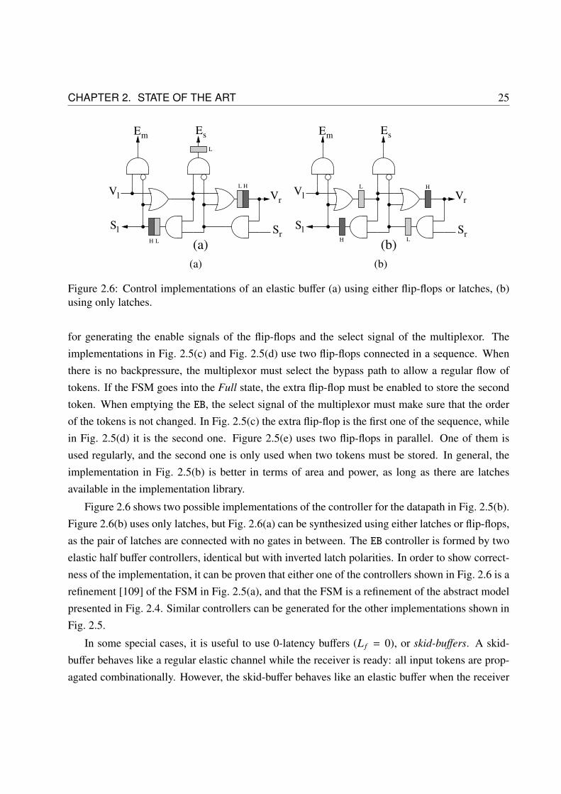
CHAPTER 2. STATE OF THE ART 25
Vl
Sl
EmEs
Vr
SrLH
L H
L
(a)
(a)
Vl
Sl
EmEs
Vr
Sr
L
H L
H
(b)
(b)
Figure 2.6: Control implementations of an elastic buffer (a) using either flip-flops or latches, (b)using only latches.
for generating the enable signals of the flip-flops and the select signal of the multiplexor. Theimplementations in Fig. 2.5(c) and Fig. 2.5(d) use two flip-flops connected in a sequence. Whenthere is no backpressure, the multiplexor must select the bypass path to allow a regular flow oftokens. If the FSM goes into the Full state, the extra flip-flop must be enabled to store the secondtoken. When emptying the EB, the select signal of the multiplexor must make sure that the orderof the tokens is not changed. In Fig. 2.5(c) the extra flip-flop is the first one of the sequence, whilein Fig. 2.5(d) it is the second one. Figure 2.5(e) uses two flip-flops in parallel. One of them isused regularly, and the second one is only used when two tokens must be stored. In general, theimplementation in Fig. 2.5(b) is better in terms of area and power, as long as there are latchesavailable in the implementation library.
Figure 2.6 shows two possible implementations of the controller for the datapath in Fig. 2.5(b).Figure 2.6(b) uses only latches, but Fig. 2.6(a) can be synthesized using either latches or flip-flops,as the pair of latches are connected with no gates in between. The EB controller is formed by twoelastic half buffer controllers, identical but with inverted latch polarities. In order to show correct-ness of the implementation, it can be proven that either one of the controllers shown in Fig. 2.6 is arefinement [109] of the FSM in Fig. 2.5(a), and that the FSM is a refinement of the abstract modelpresented in Fig. 2.4. Similar controllers can be generated for the other implementations shown inFig. 2.5.
In some special cases, it is useful to use 0-latency buffers (L f = 0), or skid-buffers. A skid-buffer behaves like a regular elastic channel while the receiver is ready: all input tokens are prop-agated combinationally. However, the skid-buffer behaves like an elastic buffer when the receiver

26 2.2. SYNCHRONOUS ELASTIC SYSTEMS
E bypass
(a)
bypass
Din
Full
Push
Dout
Empty
Pop
clk
(b)
Figure 2.7: (a) Simple skid-buffer of capacity 1 using a flip-flop, (b) skid-buffer using a syn-chronous FIFO.
applies backpressure to the channel,
Figure 2.7(a) shows the datapath implementation of a simple skid-buffer with capacity to storeone token. When there is no backpressure, the multiplexor just selects the bypass path, and theinput token is propagated to the output. On the other hand, when the stop bit is asserted, thecontrol must enable the flip-flop in the skid-buffer, and the multiplexor must change its selectionin order to preserve the order of the tokens. This skid-buffer implementation can be extended tolarger capacities. However, if the capacity of the skid-buffer is big enough, it may be more efficientto use a regular synchronous FIFO with latency 1, as shown in 2.7(b). In this case, the elasticcontrol must drive the bypass multiplexor and the control signals of the FIFO (Push and Pop). TheEmpty and Full signals must be used to compute the valid and stop signals of the controller. If theFIFO is full, the input stop signal must be asserted, and if the FIFO is empty and no token arrivesfrom the input, the output valid signal must be 0.
Forks and Joins
Elastic buffers can be generalized to any number of input and output channels by connecting addi-tional control in the inputs and the outputs. This control must be able to generate one single pairof valid and stop bits from several pairs of them, and to generate several valid and stop bits from asingle pair of them.
Figure 2.8(a) shows the control for a join structure. A pair of channels is merged into a singlechannel. The control transmits a token forward when both channels have a token, i.e., it waits forboth senders to be ready. The input channels are stopped if they have a token to transmit (their validsignal is asserted) but the token cannot be transmitted through the output channel, either becausesome of the other inputs is not valid or because the stop bit of the output channel is true.
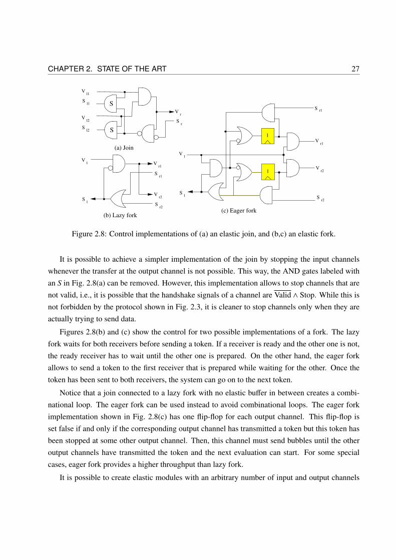
CHAPTER 2. STATE OF THE ART 27
Vr
Sr
Vl1
Vl2
Sl1
Sl2
(a) Join
Vr1
Vr2
Sr1
Sr2
Vl
Sl
(b) Lazy fork
Vr1
r1S
Vr2
S
1
1
Vl
Sl
r2
(c) Eager fork
S
S
Figure 2.8: Control implementations of (a) an elastic join, and (b,c) an elastic fork.
It is possible to achieve a simpler implementation of the join by stopping the input channelswhenever the transfer at the output channel is not possible. This way, the AND gates labeled withan S in Fig. 2.8(a) can be removed. However, this implementation allows to stop channels that arenot valid, i.e., it is possible that the handshake signals of a channel are Valid ∧ Stop. While this isnot forbidden by the protocol shown in Fig. 2.3, it is cleaner to stop channels only when they areactually trying to send data.
Figures 2.8(b) and (c) show the control for two possible implementations of a fork. The lazyfork waits for both receivers before sending a token. If a receiver is ready and the other one is not,the ready receiver has to wait until the other one is prepared. On the other hand, the eager forkallows to send a token to the first receiver that is prepared while waiting for the other. Once thetoken has been sent to both receivers, the system can go on to the next token.
Notice that a join connected to a lazy fork with no elastic buffer in between creates a combi-national loop. The eager fork can be used instead to avoid combinational loops. The eager forkimplementation shown in Fig. 2.8(c) has one flip-flop for each output channel. This flip-flop isset false if and only if the corresponding output channel has transmitted a token but this token hasbeen stopped at some other output channel. Then, this channel must send bubbles until the otheroutput channels have transmitted the token and the next evaluation can start. For some specialcases, eager fork provides a higher throughput than lazy fork.
It is possible to create elastic modules with an arbitrary number of input and output channels

28 2.2. SYNCHRONOUS ELASTIC SYSTEMS
t t
-1
Figure 2.9: Early evaluation firing in transition t, an anti-token is added to the lower input placeafter firing.
by chaining several join or fork structures. There are available algorithms that allow to minimizethe number of 2-input join and 2-output fork control components in order to optimize the controlnetwork [91].
2.2.3 Early Evaluation and Token Counterflow
[32, 34, 53] rely on lazy evaluation: the computation is initiated only when all input data areavailable. This requirement is often too strict. Consider a multiplexor with the following behavior:
z = if s then a else b.
If the value s is known, then it is only necessary to wait for the required token in order to computeo. If, for instance, s and a are available and the value of s is true, the result o = a can be producedwithout waiting for b to arrive and the value of b can be discarded when it arrives at the multiplexor.
Early evaluation takes advantage of this flexibility to improve system performance. The irrel-evant tokens with late arrival must be nullified in order to avoid spurious enabling of functionalunits. This is a key problem that must be solved correctly to guarantee that relevant data are notdiscarded by mistake. When early evaluation occurs, a negative token, also called anti-token, isgenerated in the late channels that were not used for enabling the block. When an anti-token anda token meet in the same channel, they cancel each other. Figure 2.9 shows early-evaluation firingsemantics using a marked graph model. When transition t fires, it removes one token from eachinput and adds one token to each output. Since the lower input place has no tokens initially, ananti-token is added to ensure correct token ordering.
Anti-tokens can be passive, waiting for the token to arrive inside the early evaluation joincontroller, or active, traveling backwards through the control until they meet a token. Anti-tokensfor early evaluation were already used in [92, 159], where Petri nets were extended to handle ORcausality and nodes with arbitrary early-evaluation functions.
CHAPTER 2. STATE OF THE ART 29
Several groups in the asynchronous design community have used early evaluation to allow alogic block to compute its outputs before all of its inputs are available. In [134], the inputs oflogic blocks with early-evaluation are partitioned between early and late. Once all early inputsare available a new output may be produced. However, the block must still wait for all inputs toarrive before advancing to the next evaluation. This technique has also been applied to a coarsergranularity [133]. In [6] and [21], anti-tokens flow in the backward direction and they cancelunneeded regular tokens. This token counterflow allows blocks to advance to the next evaluationwithout waiting all the inputs, achieving a higher performance. In [6], special care was taken toavoid metastability regardless of the arrival order of signals.
Several strategies have been proposed to incorporate early evaluation into latency-insensitiveprotocols [40, 49, 99]. A comparison between them can be found in [41]. A related method isproposed in [4,143] to optimize latency-insensitive systems in the presence of multi-clock domains.
In [99], a method to automatically derive don’t care conditions of the datapath logic is pro-posed. For example, when an FSM is in a certain state, its state-transition and output functionsmay only depend on a subset of its inputs. Hence, it is not necessary to wait for the rest of theinputs. This functional independence conditions (or FICs) are then used to create early-evaluationlogic that can boost-up the performance by avoiding unnecessary stalls.
In [40], latency-insensitive systems with early evaluation are called adaptive, as opposed tostatic systems when they are not early evaluated. In this work, an oracle obtains basic informationtaken from the logic block in order to select the necessary inputs for every new evaluation.
It can be considered that both [99] and [40] use passive anti-token implementations. Thus,early evaluation is handled locally, there is no extra communication between modules due to earlyenablings. When early evaluation is triggered in a module, its controller uses some internal coun-ters to remember which channels are not valid. When a token arrives to an input channel with acounter that contains some anti-token, the token is discarded and the counter decreases its value.The maximum value allowed to this counters can affect the overall performance, because earlyevaluation cannot be allowed if it will cause an overflow on the counters.
In [49], SELF is extended to handle early evaluation both with active and passive anti-tokens.The conditions for early evaluation are not derived automatically, they must be provided by thedesigner. Using this method, the usual flow of tokens is complemented by a dual flow of anti-tokensgoing in the backward direction. Elastic buffers are extended so that they can store and propagateanti-tokens the same way they store and propagate tokens. Instead of two handshake signals, fourhandshake signals are required, two of them to propagate tokens in the forward direction and the

30 2.2. SYNCHRONOUS ELASTIC SYSTEMS
Data
Valid
Stop
Sender
Receiver
Valid
Stop
+
-
-
+
Figure 2.10: Elastic channel with dual protocol. Valid+ and Stop+ propagate tokens forward, whileValid− and Stop− propagate anti-tokens backwards.
other two to propagate anti-tokens in the backward direction, as shown in Fig. 2.10. The symbolsV+, S +, V− and S − denote the valid and stop signals for the positive and negative flows. Note thatthe V− signal has the semantics of a Kill for the positive tokens.
Protocol
The SELF protocol must be duplicated in order to be able to adopt token counterflow. The V+ andS + signals implement the SELF protocol to transmit tokens and then V− and S − implement it totransmit anti-tokens in the opposite directions. In the boundaries of the EBs, tokens and anti-tokensmust cancel each other when they meet.
Furthermore, a new invariant must be complied by the elastic channels: it is not possible to killa token and to stop it at the same time. The same invariant applies to the dual channel:
V− ∧ S + and V+ ∧ S − (Dual Invariant)
Persistency and liveness properties must also be extended for dual channels. A dual chan-nel must comply the persistence property for both the forward pair of handshake signals and thebackward pair of handshake signals, and it is live if there is always more tokens or anti-tokens topropagate:
G ((V+ ∧ S +) =⇒ X V+) (Retry+)
G ((V− ∧ S −) =⇒ X V−) (Retry-)
G F ((V+ ∧ S +) ∨ (V− ∧ S −)) (Dual Liveness)

CHAPTER 2. STATE OF THE ART 31
i i+ki+1
rd wr
...B
k tokens
i i+ki+1
...B
rdwr k anti−tokens
State vars: B : array [0 . . .∞] of data; rd,wr : N; retry+, retry− : B;Initial state: wr ≥ 0; rd ≥ 0; retry+ = retry− = f alse;
Combinational behavior:
V+out =
true if retry+
f alse if rd ≥ wr
∗ otherwise
V−in =
true if retry−
f alse if rd ≤ wr
∗ otherwise
Dout =
B[rd] if V+out
∗ otherwise
S +in =
f alse if V−in∗ otherwise
S −out =
f alse if V+out
∗ otherwise
Sequential behavior:
rdnxt =
rd + 1 if (V+out ∧ ¬S +
out) ∨ (V−out ∧ ¬S −out)rd otherwise
wrnxt =
wr + 1 if (V+in ∧ ¬S +
in) ∨ (V−in ∧ ¬S −in)wr otherwise
retry+nxt = V+
out ∧ S +out
retry−nxt = V−in ∧ S −inB[wr]nxt = Din
Liveness properties (finite response latencies):Forward latency: G (rd < wr =⇒ F (V+
out ∨ V−out))G (rd > wr =⇒ F (V−in ∨ V+
in))Backward latency: G (¬S +
out =⇒ F ¬S +in)
G (¬S −in =⇒ F ¬S −out)
Figure 2.11: Abstract model for an elastic FIFO with anti-tokens.
Dual Elastic Buffers
The abstract model for an EB with token counterflow as described in Fig. 2.4 must be extendedso that the buffer can store and propagate anti-tokens, as shown in Fig. 2.11. An EB becomes anunbounded FIFO which stores tokens (data items) and anti-tokens, which cancel each other at theboundaries of the EB.
B is an infinite array that stores the tokens written to the buffer. Variables wr and rd are the

32 2.2. SYNCHRONOUS ELASTIC SYSTEMS
V + V +
S +
V -
S -
V +
S +
V -
S -
L
H
L
H
H
L
H
L
En En
S +
1
Figure 2.12: Linear pipeline with dual elastic buffers. The anti-token flow is stopped at the begin-ning of the pipeline by setting S −in to 1.
write and read pointers respectively. When wr > rd, the buffer contains k = wr − rd tokens of data.On the other hand, when wr < rd, the buffer contains k = rd − wr anti-tokens. Notice that whenthe buffer stores tokens, each incoming anti-token decrements the amount of tokens, while eachincoming token increments the number of tokens. When the buffer stores anti-tokens it works inthe opposite way. If wr = rd the buffer is empty.
The retry+ and retry− variables ensure that transmissions are persistent, as required by theprotocol. If the buffer contains no tokens (anti-tokens), no transfer can be performed, V+
out = f alse
(V−in = f alse). The cases V+out = ∗ and V−in = ∗ model the non-deterministic latency of the buffer for
propagating tokens and anti-tokens. The stop bits are asserted non-deterministically satisfying theconstraint that both tokens and anti-tokens cannot be canceled and stopped at the same time.
The liveness properties expressed in LTL ensure finite but unbounded latencies in the forwardand backward directions for both tokens and anti-tokens. The first property states that each tokenstored in the buffer must eventually be sent or killed by an anti-token (finite forward response). Thesecond property ensures a finite response time of the stop bits: each time the receiver environmentis ready to receive a new token, the buffer must eventually become ready to receive a new tokenfrom the sender. The two symmetric properties must hold for anti-tokens.
The implementation of regular elastic buffers, shown in Fig. 2.6, is substituted by the controller

CHAPTER 2. STATE OF THE ART 33
in Fig. 2.12. In Fig. 2.12, the upper layer transmits tokens forward and generates the enable signalsfor the datapath latches, while the lower layer transmits anti-tokens backwards. The shaded ANDgates cancel tokens and anti-tokens when they meet in the interface of an elastic half buffer.
Notice that token counterflow requires to duplicate the controller logic and hence the con-troller area. Therefore, active anti-tokens should only be used when they can actually provide aperformance benefit compared to passive anti-tokens. In order to stop the token counterflow, theanti-token stop bit S − is set to one and the valid bit V− is not propagated backwards anymore, asshown in the left-most anti-token controller in 2.12. If needed, an anti-token counter similar to theones proposed in [40, 99] can be introduced in any channel to increase the capacity of a buffer tostore anti-tokens.
Forks, Joins and Early Joins
When propagating anti-tokens, the join and fork structures from Fig. 2.8 are substituted by thejoin and fork structures in Fig. 2.13. The join controller in Fig. 2.13(a) is composed by a joincontroller to transmit tokens in the forward direction and a fork controller to transmit anti-tokensin the backward direction. Similarly, the fork controller in Fig. 2.13(b) is composed by a forkcontroller to transmit tokens and a join controller to transmit anti-tokens backwards. The gateslabeled with I in Fig. 2.13(a) ensure that the stop bit is not asserted at the same time that the validbit of the opposite polarity, in order to comply with the Dual Invariant rule.
The fork structures used in these dual controllers are different from the ones shown in Fig. 2.8,although they are equivalent. The main difference is the semantics of the flip-flop at each outputchannel of the fork. While the flip-flop of the original implementation is 0 if and only if the tokenwas transmitted in this channel but not in some other channel, in the dual implementation the flip-flop is 1 when the token could not be transmitted to the output channel, and hence the protocolis in retry state for this channel. This change simplifies the communication between token andanti-token transfers. The gate labeled B in Fig. 2.13(a) ensures that V+
out is not true if the forksending anti-tokens has some pending transfer. This way, the controller does not propagate tokensthat must actually be canceled.
Besides fork and join structures, an special join controller, shown in Fig. 2.13(c), is needed inorder to enable early evaluation. Consider, for example, a join controller for a 2-input multiplexor,which must be early evaluated. It would have three input channels: s, a, and b. The first channelwould be associated with the select signal. Since every channel is elastic, it would also carry the V

34 2.2. SYNCHRONOUS ELASTIC SYSTEMS
-in1
S
V -in1
-in2
V
-in2
S
V +out
+out
S
-out
S
V -out
+in2
S
V +in2
+in1
S
V +in1
FF
I
I
I
B
FF
(a)
+in
S
-in
S
V -in
V +out2
V +out1
+out1
S
+out2
S
V +in
-out1
S
V -out1
-out2
S
V -out2
FF
FF
(b)
V +out
+out
S
-out
S
V -out
-in1
S
V -in1
-in2
V
-in2
S
V +in1
+in2
S
V +in2
+in1
S
G
G
FF
FF
EE
data
(c)
Figure 2.13: (a) dual elastic join, (b) dual elastic fork, (c) dual elastic join with early evaluation.
CHAPTER 2. STATE OF THE ART 35
and S signals of the elastic protocol. The enabling function (block EE in Fig. 2.13(c)) would be:
EE = V+s ∧ ((s ∧ V+
a ) ∨ (s ∧ V+b )) (2.2)
The signal s corresponds to the data value of the channel with the same name. Note that V+s
must always be true for the enabling of the module. An early enabling is produced, for examplewhen V+
s = V+a = 1 and s = 1. In this case, if V+
b = 0, an anti-token will be produced in thechannel b. The gates labeled with G in the controller are responsible for generating such anti-tokens if necessary. These anti-tokens can travel backwards through a dual controller, or they canbe stored locally in a counter. This controller can be optimized in some special cases by usingtoken cages [38].
In order to ensure that the SELF protocol is complied by the controller, the cofactors of the EEfunction with respect to data inputs must be positive unate for the valid signals. In other words, EEcan check for the presence of tokens, but never for their absence. For the previous example, thecofactors with respect to the data input s are:
EEs = V+s ∧ V+
a EEs = V+s ∧ V+
b (2.3)
Feedback paths from datapath to controller and back to the datapath must be designed carefully.If the output channel of an early-evaluation controller is connected to the input channel of an elasticbuffer, a combinational path appears from the data input of the early-evaluation controller to theenable signal of the latch of the elastic buffer. Since the datapath latch is active low and the inputprobably comes from an active high latch or from a flip-flop, this combinational path must arrivein half cycle. Depending on the width of the EB (the number of actual one bit latches driven by thisenable signal), the number of logic levels before the early join controller and the complexity ofthe EE function, this path might become critical. This potential problem must be considered whenimplementing early evaluation. The path from the valid bit to the enable signal of this critical latchcan be removed to alleviate this problem. Then, the latch will always capture new data unless it isstopped, but correctness is still preserved.
2.2.4 Verification
Designing controllers for elastic systems is difficult and error-prone. It must be ensured that thedesigned controllers comply with the specified protocol (e.g., see [50,100]). This is typically done

36 2.2. SYNCHRONOUS ELASTIC SYSTEMS
A B C
EB EB EBvalid
stop
valid
stop
(a)
0 1 2 3 4 5 6 7 8 . . .
A 0 1 1 0 1 1 0 1 1 . . .
B 1 0 1 1 0 1 1 0 1 . . .
C 1 1 0 1 1 0 1 1 0 . . .
(b)
A B C
0 1 1 1 0 1 1 1 0
(c)
Figure 2.14: (a) Simple synchronous elastic pipeline, (b) Simulation trace for each of the elasticbuffers of the example during some cycles, 0 means the EB does not store a new token, 1 meansthe EB stores a new token, (c) system implemented using scheduling.
using some formal verification tool like NuSMV [44].
It must be verified that all elastic channels comply with the protocol. In the case of SELF,persistence and liveness must be proven. For dual channels, persistence must be verified both fortokens and anti-tokens, and the dual invariant must also be verified (a token is never stopped andcanceled). It is also important to prove a correct interaction with the datapath to make sure that notokens are lost.
In [148], a framework for validating families of latency-insensitive protocols is proposed. Theoutput behavior of the original system and the output behavior of the elasticized system are com-pared on a subset of possible inputs, allowing quick debugging of new protocols without an ex-haustive verification.
It must be ensured that functionality is not lost when transforming a synchronous system intoa latency-insensitive one. In [32], it is proven that if all modules of a synchronous system arereplaced by the corresponding latency-insensitive modules, the resulting system is patient andlatency equivalent to the original one.
Similar results are proven in [96] for synchronous elastic systems. Furthermore, it is shownthat when a set of correct elastic systems are composed, they form a new correct elastic system. Itis also shown that empty EBs can be added without modifying the functionality of the system.
In [146] a refinement technique is suggested for verifying that an optimized elastic systemcomplies with the original specification. Although it does not apply to systems with early eva-luation, it can still be used to prove that an elastic system with bubbles is equivalent to the initialdescription of the design.

CHAPTER 2. STATE OF THE ART 37
2.2.5 Scheduling
Latency-insensitive designs with only late-evaluation modules tend to have a fixed repetitive be-havior [19, 39]. This means that the values for valid and stop bits in the control can actually bepredicted a priori. Then, the control logic for each elastic buffer can be reduced to a simple ring ofappropriately initialized registers.
Consider the simple example pipeline in Fig. 2.14(a). This pipeline has three elastic buffersconnected forming a ring. Initially, EBs A and B contain a token, while C is a bubble. Considerthe simulation trace shown in Fig. 2.14(b). In the first clock cycle, B and C receive a new token.However, A does not store a new token because C has no token to transmit. On the second cycle, A
and C receive new tokens, while B receives a bubble. On the fourth cycle, the configuration is thesame as in the first cycle, and from then on the behavior repeats itself. The throughput is 2/3 sinceevery three cycles, two tokens are received by each elastic buffer.
It is possible to synthesize a schedule for each elastic buffer of the design, using some of thealgorithms described in [19, 39]. Then, the system can be implemented by using a scheduledcontrol, as shown in Fig. 2.14(c). This implementation does not need any handshake signals. Theschedule of each elastic buffer is an automaton the decides, each clock cycle, whether to enable theelastic buffer by following the cyclic sequence described by the schedule.
The main advantage of scheduling latency-insensitive designs is that it removes the need toroute the valid and stop wires. These wires may potentially be long and become a problem forrouting. However, if the resulting schedule is too long, the area may actually increase as a sideeffect. Since it is very likely that many of the EBs have the same or shifted schedule, some schedulescan be shared to reduce the area overhead [37]. Notice that sharing of schedules can only be appliedto EBs that are placed close to each other on the design. In general, systems with early evaluationdo not have a repetitive behavior and hence a scheduling cannot be found. If the selection of inputsin each of the early evaluation nodes was predictable and repetitive, then it should still be possibleto find a schedule.
2.2.6 Granularity of elastic islands
Elasticity can be applied at different levels of granularity. One option is to view a design as acomposition of large synchronous blocks with elastic communication between them in order to usemodularity or power advantage of running blocks at different clock frequencies or in anticipation ofdesign variations in communication channels. This block level view using different forms of elastic

38 2.2. SYNCHRONOUS ELASTIC SYSTEMS
EBCONTROL
vs
Lcomblogic
EBCONTROL
vs
Lcomblogic
EBCONTROL
comblogic
L
JOIN vs
Figure 2.15: Elastic system with 3 IP blocks that have been elasticized by adding an elastic wrapperaround them. The control wires are marked with dotted lines.
shells around existing blocks is presented in [34], [152], and [52, §8]. This kind of granularitytargets mainly SoC designs.
For example, Fig. 2.15 shows an elastic system where 3 existing synchronous blocks have beenelasticized. The global clock of each block is substituted by the gated clock generated by the EBcontroller. Thus, the elastic controller commands all the registers of the block with only one enablesignal. Backpressure is handled by adding ghost latches at the inputs of the blocks. These latcheshave the same polarity as the internal input latches of the block and do not introduce any extralatency, since they are redundant during the normal operation of the system. The ghost latch andthe elastic control are the wrapper that must be added to each block to transform it into a pacientshell.
On the other extreme, one can consider a synchronous system as a set of gates. Every gate isthen viewed as an elastic island and the system can be redesigned to become elastic at the gatelevel. Then, each gate has associated handshake signals that communicate with each other in orderto properly transmit data. Such low level of granularity would have a prohibitive cost due to theoverhead of the huge elastic controller it would require.
An intermediate option is to view the design at the register transfer level and consider everyregister as an object of interest. Each sequential element at the RTL level is assigned to an elastic

CHAPTER 2. STATE OF THE ART 39
buffer (or relay station) controller, and the synchronization between elastic buffers is extracted bytheir data-flow dependencies in the RTL design. This view is similar to the one used in the classicalretiming optimization, and can be used for elastic systems of the size of a microarchitecture. Evenwith focus on the RTL level, it is possible to easily group different registers together or decomposethem if it is beneficial for performance or area of the design. Using this approach, it is still possibleto integrate IP blocks in the design with elastic shells as in the block level approach.
2.2.7 Synthesis Flow
This section describes a synthesis flow that can be used to transform a rigid synchronous systeminto a synchronous elastic system. This flow is based on the one presented in [36]. Similar flowsfor synchronous elastic designs have been presented in [31, 53, 82]. It can also be used for desyn-
chronization, i.e., to transform a synchronous design into an asynchronous one [20, 54, 93, 151].This flow can be implemented in an EDA tool and it should be applied during synthesis of
the design (either before synthesis on a pre-synthesized RTL or after synthesis on a synthesizednetlist). It can also be applied on the initial stages of physical design, but some features like addingbubbles may be less effective on an already placed design. The steps that must be applied are thefollowing ones:
1. Group flip-flops into multibit registers. Each group will be controlled by an EB controller.This grouping (or clustering) determines the level of granularity of the design. Some IPblocks or blocks with a very specific implementation may be kept as is, and they will beelasticized using a coarser granularity. This decision can be taken by a designer or by somealgorithm using a set of rules or heuristics. Clear candidates for coarse elasticization areregister files or memories.
2. Remove the clock signal and replace each flip-flop with the datapath implementation of an EB(a pair of latches for SELF). In the case of blocks that are elasticized at a coarser granularity,add a wrapper around it to create a shell, i.e., add a ghost latch as shown in Fig. 2.15.
3. Apply transformations to the datapath that will improve the performance of the elastic sys-tem, like adding bubbles. All the optimizations that are presented in this thesis can be appliedon this stage of the synthesis flow. In particular, early evaluation can be added by identify-ing early enabling conditions in the datapath and defining which signals must be sent to thecontroller to recognize such early firings.

40 2.2. SYNCHRONOUS ELASTIC SYSTEMS
4. Create the control layer to generate the enable signals for the latches. It must have thefollowing components:
(a) An EB controller for each EB (including blocks that have been elasticized at a coarsergranularity). The EB controller must be initialized with the correct number of tokensdepending on whether it is a bubble or not.
(b) a Join controller at the input of each EB that receives data from multiple EBs.
(c) a Fork controller at the output of each EB that sends data to multiple EBs.
Each join controller might become an early-evaluation join controller. This decision can betaken by a designer or by some algorithm that must decide whether it is wise to apply earlyevaluation given the datapath and the expected latencies of each of the input branches of thejoin. At this stage the controller can be synthesized and optimized.
5. Connect the datapath with the controller. The enable signals generated by each EB mustbe connected to the corresponding items in the datapath, and the datapath signals used byearly-evaluation multiplexors must be connected to the early-evaluation joins.
Figure 2.16 illustrates the presented synthesis flow on a simple pipeline example. In Fig. 2.16(b),the flip-flops from the original synchronous design shown in Fig. 2.16(a) have been substituted bypairs of latches in order to implement an EB. The register file in the example (RF) has 4 inputs,write address, write data, read address and read data (wa, wd, ra, rd respectively). Since registerfiles are complicated blocks where it may not be possible to substitute all flip-flops by latches, theyshould be elasticized by adding a ghost latch at its inputs.
Figure 2.16(c) shows the whole elastic system after creating the controller and connecting itto the datapath. The multiplexor at the output of the register file has been implemented as anearly-evaluation multiplexor. Hence, its select signal is connected to the controller and the join isimplemented as an early-evaluation join.
If all paths starting on the read address input of the register file are combinational paths goingto the read data output, then its input ghost latch is not necessary. In this case, the implementationshown in Fig. 2.16(d) can be used. The sender of the read address is synchronized with a join atthe EB that receives data from the register file. This implementation can be extended to multipleread and write ports and it can be used for memories as well.

CHAPTER 2. STATE OF THE ART 41
nextPC
DEC
RF
A B
wa ra
wd rd
clk
(a)
nextPC
DEC
RF
A B
wa ra
wd rd
(b)
nextPC
DEC
RF
A B
wa ra
wd rd
EB
EB
J
F EB
EBEJ EB F
F
EB
(c)
RFwa ra
wdrd
EB
EBEBJ
(d)
Figure 2.16: (a) Simple synchronous pipeline, (b) Pipeline after converting flip-flops to EBs usinga pair of latches, the register file is elasticized using a ghost latch, a bubble has been added afterthe instruction decoder (c) synchronous elastic system with controller; J means join, F fork and EJearly join; EB controllers are marked with a dot if they initially contain a token; paths from controlto datapath and from datapath to control are dashed, (d) alternative way to elasticize the registerfile if the path from read address to read data is purely combinational.
2.2.8 Modeling Elastic Systems with Marked Graphs
Petri nets can model distributed concurrent computations and their synchronization, and hence,they are an ideal model for both asynchronous systems [112] and synchronous elastic systems [51].Petri nets are well defined mathematical entities. Therefore, they have been used by several asyn-chronous groups for performance evaluation, validation, verification, formal reasoning or synthesisof asynchronous systems. Most of these applications can also be used in synchronous elastic sys-

42 2.2. SYNCHRONOUS ELASTIC SYSTEMS
A B C
EB EB EBvalid
stop
valid
stop
(a)
A B C
=1� =1� =1�
(b)
JEB
F
�A
B
C
D
EB
EB
EB
(c)
=1� =1�
=1� =1�
(d)=1�
=0�
=1�
=1� =1�
=0�
(e)
Figure 2.17: (a) Simple elastic pipeline and (b) its elastic marked graph model, each pair of placesrepresent an elastic buffer, the upper place is the forward place and the shadowed lower place isthe backward place, which represents available capacity, (c) elastic buffer with joins and forks and(d) its elastic marked graph model, (e) equivalent elastic marked graph with join and fork structureexplicitly modeled.
tems.
Since synchronous elastic systems do not have choices, marked graphs have enough expressionpower to describe them. An Elastic Marked Graph (EMG [51]) is a timed marked graph where thetime assigned to transitions is a natural number, since time represents the latency of elastic buffers,which is discrete.
EMGs label each place as a forward place or a backward place (L : P −→ {F, B}). Forwardplaces store data tokens that are stored on elastic buffers and are available to be computed by atransition. Backward places store tokens that represent available capacity of elastic buffers that canbe filled with new arriving tokens.
Thus, an elastic buffer is modeled with a forward place and a backward place. For every placep, there exists p′, such that •p = p′•, •p′ = p• and L(p) = F iff L(p′) = B. The total capacityof the buffer can be found by adding the number of forward tokens plus the number of backwardtokens.

CHAPTER 2. STATE OF THE ART 43
The example in Fig. 2.17(b) has three elastic buffers, A, B and C. In the model, each of themhas two places, one in the forward direction and one (shadowed) in the backward direction. SinceC is a bubble, initially it has two available spots to receive tokens (the backward place has twotokens) and it contains no tokens in the forward place. A full EB would have two tokens in theforward place and no token in the backward place. The other EBs are half full, and hence they haveone token at each place. Since the number of tokens per cycle is a constant in marked graphs, itis ensured that each EB will at most have as many tokens as its capacity. When a data token istransmitted in the forward direction, it can be considered that a bubble (that is, available capacity),is being transmitted in the backward direction. For example, if B sends a token to C in the example,it can also be considered that B obtains a bubble from C.
Figure 2.17(b) shows a linear pipeline. If the elastic system contains join and fork structureslike in Fig. 2.17(c), there must be a pair of places (a forward and a backward place) for each EBto EB connection, as shown in Fig. 2.17(d). If the specific join-fork structure must be modeled inthe TMG, for example, because one of the joins is an early join or some transition has a variablelatency, the backward places must still go from EB to EB, as shown in Fig. 2.17(e).
Early evaluation can be modeled with Multi-guarded marked graphs (GMG, [49, 85]). Multi-guarded MGs allow firing of some transitions even if some of the input places have no tokens.Each early-evaluation transition is assigned a set of guards, which is a subset of its input places.After each firing, the transition chooses non-deterministically one of its guards. Once all the inputplaces of the selected guard have tokens, a new firing can occur. An anti-token is inserted to eachinput place that was empty when the firing happened. Then, the next guard is selected. Each guardselection is independent.
2.2.9 Performance Analysis of Elastic Systems
The marked graph model of an asynchronous system can be used for performance evaluation. Theperformance of an asynchronous system is determined by its cycle time, i.e., how often a token istransferred through a transition. Evaluating the throughput of a synchronous elastic system is ananalogous problem to computing the cycle time of an asynchronous system. The difference is thatin asynchronous designs the time of the transitions model actual time (e.g. picoseconds), while insynchronous elastic systems the transitions model latency in clock cycles.
The asynchronous community has found multiple techniques to evaluate the performance ofa system. There are methods based on analysis of Markov processes [97, 156], linear program-

44 2.2. SYNCHRONOUS ELASTIC SYSTEMS
=1� =1� =0�
=1�
=1�
=1�
=1�
=1�
Figure 2.18: TMG model of a synchronous elastic system with two cycles.
ming [30, 46] graph structure of the marked graphs [15, 131, 132, 154], simulation-based tech-niques [28, 110, 118, 157], partial order between events [42, 80], max-plus algebra [70] or hierar-chical methods [67].
One of the most used techniques is based on an analysis of the marked graph structure. Con-sider a single ring of EBs, as shown in Fig. 2.17(b). Its throughput is determined by its token-delayratio, i.e., the number of tokens it has divided by the number of clock cycles needed to traversethe ring (the latency of the ring). For example, the throughput of the design in Fig. 2.17(b) is 2/3,since there are 2 tokens and they need 3 clock cycles to return to their starting point. This meansthat each EB transmits a token 2 of every 3 clock cycles, or that the average separation betweenconsecutive transmissions on the same channel is 1.5 (3/2).
It can be proven that the throughput of a TMG is equal to the throughput of the slowest simplecycle [131, 132]:
Θ = minc∈CM0(c)∑t∈C δ(t)
For example, the TMG in Fig. 2.18 has two simple cycles, the upper one, with a latency of5 clock cycles and 4 tokens, and the lower one, with a latency of 4 clock cycles and 3 tokens.

CHAPTER 2. STATE OF THE ART 45
The backpressure places have been removed for simplicity. The throughput of the cycles are,hence, 4/5 and 3/4, and the overall throughput is their minimum, 3/4. There are efficient poly-nomial algorithms that allow to compute the minimum token-delay ratio without enumerating allcycles [57, 89].
The fact that the slowest cycle is the one that determines the throughput can also be translatedinto a linear programming formulation [30]. In this formulation, the average marking of each placeis computed, i.e., how much time a token spends on each place on average. It is known that thethroughput multiplied by the delay of a transition must be less or equal than the average marking ofall the input places of this transition. Thus, the throughput can be found by solving the followingLP problem:
maximize: Θ,
subject to: δ(t) · Θ ≤ m(p), ∀t ∈ T, ∀p ∈ •t
m = m0 + C · σ
(2.4)
where m is the average marking, which allows real numbers, m0 is the initial marking, σ is afiring count vector which also allows real values and C the incidence matrix of the MG.
Throughput evaluation of systems with early evaluation is much more complicated. Let usassume that the shadowed transition in the example in Fig. 2.18 is early evaluated, and it chooseseither the input from the upper branch or the input from the lower branch. Each guard must beassigned a probability in order to estimate the performance. In practice, it can be assumed thatguards are formed by a single input [85]. Hence, each input is assigned a probability. For example,the upper branch is taken with probability α and the lower branch is taken with probability 1 − α.These probabilities would be determined by profiling the benchmarks expected to be executed onthe elastic system.
With early evaluation, the throughput is no longer determined by the slowest cycle. Further-more, it is not determined by the mean of the throughputs of each cycle even for simple cases.For the example in Fig. 2.18, the simple cycles have throughputs 3/4 and 4/5. However, the overallthroughput is not α ·4/5+(1−α) ·3/4, it is 3+α
4+α, determined by analyzing the Markov chain [155] of
the system, as explained in [85]. This is the only known method to compute the exact throughput,but it suffers from exponential state explosion. The previous linear programming formulation isadapted in [85,86] to support early evaluation. It provides an upper bound of the throughput, and itis usually capable of providing a correct order when measuring the performance of different elasticsystems, i.e., if pipeline A has better performance than pipeline B, then this method will also find

46 2.3. AUTOMATIC PIPELINING
that A is better than B for most of the cases. The linear programming problem cannot model activeanti-tokens.
2.3 Automatic Pipelining
A few automatic and semi-automatic pipelining approaches have been discussed in the literature.The high-level synthesis community described scheduling and resource sharing algorithms
(e.g. [126]) for functional pipelining and software loop pipelining, but static schedules cannothandle dynamic dependencies.
It has also been shown how to automatically pipeline logic blocks without adding latency usinga negative/positive register pair [73]. The output of the negative register must either be precom-puted or predicted. However, this is not possible within a critical loop (unless an expensive un-rolling operation is attempted).
[106] and [95] address the problem of verifying a pipeline via deconstructing it using term-rewriting to derive an equivalent ISA model. [106] applies microarchitectural rules without usingprecise design on its timing and control. [95] describes a method to add forwarding logic and stallengine to a specification already partitioned into stages. The manual design needs to be proved forcorrectness afterwards. They use a global controller that needs to send data to all stages. Globalcontrollers that handle stalling and logic forwarding may introduce critical paths in the control ofdesign and are generally not acceptable in the nanometer technologies.
[105] extracts operations from a specification in the form of term-rewriting rules [77], andschedules them into stages interconnected via FIFO queues. Speculation, stalling and forwardingare accomplished by specific styles of rewriting. It is also implemented by using a global controller.
[78] uses term-rewriting rules in order to specify a high-level description of a design, andthen the specification is automatically synthesized into a synchronous elastic system, which has adistributed controller.
[76] proposes a framework to specify and verify pipelines where designers follow a templateto specify pipeline stages and choose from a library of control cells. As a result, verificationscripts about pipeline properties can be generated automatically. Their approach does not useprovably-correct transformations and does not generate optimal stalling and bypass based on datadependencies.
[111] proposes a method to explore different possible pipelines starting from an architecturalspecification. Transformations such as addition of pipeline stages, pipeline paths, opcodes and

CHAPTER 2. STATE OF THE ART 47
new functional units are supported. However, some manual work is required in order to identifyand insert forwarding paths. They focus only on instruction set processors, and hence they cannotpipeline arbitrary sequential datapaths.
[121] presents a method to automatically synthesize a pipeline from a transactional datapathspecification. The specification executes one instruction (or transaction) at a time. Each module ofthe specification is then assigned to a stage automatically forming a pipeline. Possible forwardingpaths are automatically discovered by the tool, and then the user can choose which forwardingpaths to include in the pipeline. The user can also provide value predictors for some modulesso that speculative execution can be inserted if necessary. Data hazards that cannot be solved byforwarding or speculation are solved by stalling the pipeline using a handshake mechanism similarto a latency-insensitive design. The final pipeline preserves the original transaction semantics butallows parallelism by executing multiple overlapped transactions across pipeline stages. In [122]this method is extended to allow in-order multi-threading.
2.4 Conclusions
This chapter has given an overview of the notions needed to understand this thesis. Synchronouselastic systems have been presented, and its specification, synthesis, verification and analysis havebeen discussed. Finally, the chapter also provides a review of automatic pipelining methods.

48 2.4. CONCLUSIONS

Chapter 3
Correct-by-construction Transformations
This chapter collects a set of transformations that can be applied to an elastic design. All transfor-mations are correct-by-construction: it is guaranteed that functionality will be preserved throughthe exploration of different possible microarchitectures. However, the latency of computations andcommunications may change since the advantages of synchronous elastic systems are used. Ap-plying these transformations to a conventional sequential circuit would be possible, but difficultand error-prone, since it would be necessary to emulate an elastic system with some controller.These transformations can be used for automatic exploration of elastic pipelines.
Most of the transformations have been already used in other contexts. The novelty of thischapter is that it gathers all of them so that they can be used together to perform microarchitecturalexploration. First, the microarchitectural graphs used throughout this work and the toolkit that hasbeen built to manipulate them are presented. Then, a set of latency-preserving transformations isintroduced. Next, the set of transformations that are only correct for elastic systems is discussed.Finally, verification of such transformations is discussed. The contributions of this chapter havebeen published in [87] and in [48].
3.1 Introduction
One of the major features of synchronous elastic systems is their tolerance to latency changes. Suchtolerance can be used to design systems optimized for the typical case (in terms of data variability)instead of the worst case. For example, an ALU can be redesigned so that it can compute operationswith small operands in one clock cycle, while long operations will halt the computation flow and
49

50 3.1. INTRODUCTION
Figure 3.1: Sequence of correct-by-construction transformations applied to a design.
take one extra cycle. Using this variable-latency ALU, the cycle time can be reduced, and assumingthe extra cycle is not required too often, an overall performance improvement will be achieved.
An elastic system can be abstracted as a graph where the nodes represent computational blocksand the edges represent channels that transmit data between these blocks. Edges may containelastic buffers.
Under this abstraction, the transformations that will be presented in this chapter take an elasticgraph and modify a small subset of this graph. The resulting graph is latency equivalent to theinitial graph, i.e., if idle cycles are ignored, the streams of data on each input and output channelare the same.
By applying a sequence of small steps that perform local transformations to different parts ofthe design, it is possible to traverse the space of designs that are latency equivalent to the orig-inal design, as show in Fig. 3.1. After several transformations, it may not be obvious to deter-mine whether the current design keeps any kind of relation with the original one. However, thefact that all transformations are correct-by-construction and preserve latency equivalence assuresthat functionality remains unchanged. The optimization of elastic systems by using correct-by-construction transformations can be applied on the third step of the synthesis flow presented inSection 2.2.7.

CHAPTER 3. CORRECT-BY-CONSTRUCTION TRANSFORMATIONS 51
F
W R
wa
rd
ra
wdk
-knode representing a functional unit
skid-buffer with capacityto store k tokens
elastic buffer with one token(capacity=2, latency=1)
empty elastic buffer (bubble)(capacity=2, latency=1)
channel with an anti-tokeninjector with k anti-tokens
abstraction of a register filewith one write port and oneread port
early evaluation multiplexorwith 2 input data channels
(a)
FW R
G
+D
(b)
Figure 3.2: (a) Notation to represent elastic microarchitectural graphs, (b) microarchitectural graphexample.
3.2 Microarchitectural graphs
Elastic microarchitectures are described in this work using directed multigraphs, which modelthe Control Data-Flow Graph of the design. A directed multigraph is a directed graph which ispermitted to have multiple edges from the same source to the same target. More formally, it is agraph G = (V, A) where V is a set of nodes and A, the arcs of the graph, is a multiset of orderedpairs of nodes.
Microarchitectural graphs can be derived from an actual design, by capturing the graph struc-

52 3.2. MICROARCHITECTURAL GRAPHS
ture of the circuit at some level of granularity, or from a functional specification of an InstructionSet Architecture, ISA.
The nodes of the graph correspond to functional units. Each node is assigned an area, a combi-national delay and a latency. The latency can be a natural number or a set of natural numbers eachone with an associated probability if the node is implemented as a variable-latency unit.
Some nodes may have additional attributes in order to enable early evaluation, sharing of func-tional nodes, register files, memories, environment nodes and generic IP modules.
The arcs of the multigraph represent elastic channels that transfer data between a sender nodeand a receiver node. The arcs may contain EBs, skid-buffers and anti-token counters. Each arc isassigned a latency (which determines the number of EBs), a capacity to store tokens, a capacity tostore anti-tokens, and an initial number of tokens. The initial number of tokens is an integer whichcan be negative if the channel initially contains anti-tokens.
Figure 3.2(a) shows some notation used in order to represent elastic microarchitectural graphsin this work. Control details are not explicitly displayed, only the data dependencies are drawn.Elastic buffers are represented as boxes. If the EB is initialized with one token a dot is drawninside the box. EBs are assumed to have one clock cycle of latency and the ability to store twotokens. Skid-buffers are represented by rhombus, labeled with their capacity. Anti-token injectorsare drawn as a pentagon under the elastic channel, labeled with the number of anti-tokens in theanti-token counter. Early-evaluation multiplexors are drawn as a regular multiplexor. At a certainlevel of abstraction, a register file can be represented by a monolithic register and additional logicto write (W) and read (R) data. The wires wd and rd represent data, whereas the wires wa and ra
represent addresses. The actual implementation of the register file within the elastic system wouldbe as discussed in Section 2.2.7.
Figure 3.2(b) shows an example of a microarchitectural graph. There is one register file andone multiplexor selecting between two data inputs. There are four functional nodes, one addingtwo values and labeled with the plus symbol, two nodes connected in a pipeline and another onewhich outputs to the select signal of the multiplexor and the write and read addresses of the registerfile. The data that has not been drawn in this figure are the area, delay and latencies of the nodes,plus the probabilities for each of the inputs of the multiplexor. They are needed in order to evaluatethe performance of the design.
The microarchitectural graphs can be hierarchical, i.e., a node may contain another graph in-side. The internal contents of a node may be exposed depending on the level of granularity to beapplied to the elastic system. For example, a node may represent an ALU, and it may contain an-

CHAPTER 3. CORRECT-BY-CONSTRUCTION TRANSFORMATIONS 53
other microarchitectural graph with a description of the implementation of the ALU (e.g., an adderand a multiplier connected to an early-evaluation multiplexor). Then, it is possible for the user todecide whether to elasticize the ALU as a whole or to insert transformations inside the ALU tofurther optimizer the system. Hierarchy allows description of larger graphs.
3.3 Toolkit
A tool named MAREX has been built to describe and manipulate microarchitectural graphs. Inorder to interact with the tool, the user enters command scripts within an interactive shell, in flavorof other systems with interactive interfaces (e.g. SIS [139] or ABC [1]). Scripts can also beexecuted in batch mode. The core of MAREX is written in C++ for a performance reason, whilePython is used as the front-end for interactive use. In total, MAREX contains around 40K lines ofcode, developed for the most part by the author of this thesis.
MAREX can apply correct-by-construction transformations on its graphs, visualize the modi-fied graph, undo and redo the transformations, etc. Since most transformations are local, i.e. theyare applied on a small sub-graph, they are very fast to compute. Longer scripts that compose asequence of transformations or implement more complex algorithms can be built as well.
The cycle time of the graph can be computed by traversing the graph using the delays associatedto the nodes. It is possible, at any point, to compile the microarchitectural graph into a Verilognetlist of the elastic controller, a marked graph for performance analysis, as explained in [25], a blifmodel for logic synthesis with SIS [139] or a NuSMV [44] model for verification. Other modelsfor global optimizations like EB capacity sizing or retiming and recycling can also be generated.The elastic controller is built by assembling the set of predefined parameterized control circuitprimitives presented in Section 2.2. Verific’s front-end library for manipulating Verilog is used togenerate the controller RTL. For calculating performance of the design point the Verilog netlist ofthe elastic controller and the specified model of the datapath is simulated and the throughput isobtained. The throughput can also be estimated by generating a marked graph and analyzing itsperformance.
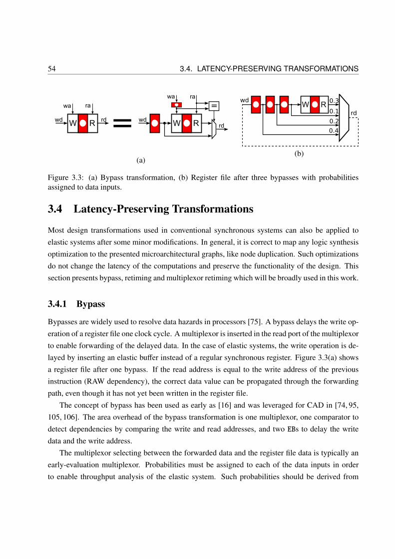
54 3.4. LATENCY-PRESERVING TRANSFORMATIONS
W R
wa
rd
ra
wd W R
wa
rd
ra
wd
=
=(a)
W Rrd
wd 0.3
0.1
0.2
0.4
(b)
Figure 3.3: (a) Bypass transformation, (b) Register file after three bypasses with probabilitiesassigned to data inputs.
3.4 Latency-Preserving Transformations
Most design transformations used in conventional synchronous systems can also be applied toelastic systems after some minor modifications. In general, it is correct to map any logic synthesisoptimization to the presented microarchitectural graphs, like node duplication. Such optimizationsdo not change the latency of the computations and preserve the functionality of the design. Thissection presents bypass, retiming and multiplexor retiming which will be broadly used in this work.
3.4.1 Bypass
Bypasses are widely used to resolve data hazards in processors [75]. A bypass delays the write op-eration of a register file one clock cycle. A multiplexor is inserted in the read port of the multiplexorto enable forwarding of the delayed data. In the case of elastic systems, the write operation is de-layed by inserting an elastic buffer instead of a regular synchronous register. Figure 3.3(a) showsa register file after one bypass. If the read address is equal to the write address of the previousinstruction (RAW dependency), the correct data value can be propagated through the forwardingpath, even though it has not yet been written in the register file.
The concept of bypass has been used as early as [16] and was leveraged for CAD in [74, 95,105, 106]. The area overhead of the bypass transformation is one multiplexor, one comparator todetect dependencies by comparing the write and read addresses, and two EBs to delay the writedata and the write address.
The multiplexor selecting between the forwarded data and the register file data is typically anearly-evaluation multiplexor. Probabilities must be assigned to each of the data inputs in orderto enable throughput analysis of the elastic system. Such probabilities should be derived from

CHAPTER 3. CORRECT-BY-CONSTRUCTION TRANSFORMATIONS 55
F F=(a)
0F F
(b)
F F=
(c)
Figure 3.4: (a) Retiming transformation, (b) adding a fake fork to enable sharing of elastic buffers,(c) invalid elastic retiming.
profiling the benchmarks expected to be run on the microarchitecture. It must be determinedhow often a data dependency can occur for every possible timing distance between instructions,i.e., for instructions that are executed consecutively, for instructions that are executed with oneinstruction in between, with two instructions in between, and so on. This way, multiple bypassescan be applied and the corresponding probabilities can be assigned to each new early evaluationmultiplexor.
Figure 3.3(b) shows a register file with three bypasses and assigned probabilities. The readand write address modules have been ignored for simplicity. The output of the early-evaluationmultiplexor may eventually write back to the register file, as shown by the dotted line. In thisexample, it has been determined that the running instruction will require the value written by theprevious instruction with probability 0.4, the value written two instructions ago with probability0.2 and three instructions ago with probability 0.1. Therefore, there will be no data dependencieswith probability 0.3.

56 3.4. LATENCY-PRESERVING TRANSFORMATIONS
4 4
1 2
3 983
9
(a)
4 4
1 2
3 983
9
(b)
Figure 3.5: Design optimized using (a) Retiming, (b) Retiming and recycling.
3.4.2 Retiming
Registers can be moved across combinational logic preserving the functionality, as shown inFig. 3.4(a), where a register is moved through node F. Retiming [98] is a traditional techniqueof sequential delay and area optimization. It can also be used to reduce the power consumption ofa system [113].
When applying retiming to a synchronous elastic system, it must be ensured that the re-timed registers have the same number of initial tokens. For example, the transformation shownin Fig. 3.4(c) is not valid since one of the EBs is a bubble and the other one is not.
The optimization problem of minimizing the cycle time of a design using retiming can besolved in polynomial time [98, 137, 141]. If the target is to minimize the area (i.e., the numberof registers) under some timing constraints the problem becomes NP-complete [98], although itmay be solved efficiently in some particular cases [81]. The results for area minimization can beimproved by adding a fake fork node with zero delay [98, 136], as shown in Fig. 3.4(b). All thesemethods can be applied to the EBs of synchronous elastic systems. Since the initial state of thecircuit may be changed by retiming, a new initial state must be computed after retiming to ensurecorrect initialization. This is always possible if the retiming graph is strongly connected [150].
Figure 3.5(a) shows an example with an optimal retiming. The combinational nodes (shown ascircles) are labeled with their delays. The cycle time of this design is 17 time units, determined bythe two nodes with delays 9 and 8 in the lower right corner.

CHAPTER 3. CORRECT-BY-CONSTRUCTION TRANSFORMATIONS 57
F = FF
a
b
c
xa
b
c
x
(a)
=(b)
Figure 3.6: (a) Multiplexor retiming and (b) bubble insertion.
3.4.3 Multiplexor Retiming
Functional units can be retimed through multiplexors by adding one copy of the functional unit toeach data input of the multiplexor, as shown in Fig. 3.6(a). Such transformation can be used tomove logic out of a loop going from the output of a multiplexor to its control channel, similar towhat is proposed in [144].
It is easy to show that x in the figure is the same function before and after the transformation,using cofactors and Shannon decomposition:
x = F(c′a + cb) (3.1)
= c′Fc′(c′a + cb) + cFc(c′a + cb) (3.2)
= c′F(a) + cF(b) (3.3)
3.5 Recycling
Recycling is a transformation that changes the latency of an elastic channel. It is always possibleto insert and remove an empty EB (a bubble) on any channel of an elastic system (for formal proofsee [96]). This transformation is shown in Fig. 3.6(b).
Bubble insertion is also known as recycling, and was initially introduced in [33]. In syn-chronous elastic designs, recycling can be combined with retiming leading to a more powerfuldesign optimization [26, 35]. Reducing the cycle time of the elastic system by inserting bubblesusually yields to a lower throughput since there are fewer tokens per cycle. By properly balancingcycle time and throughput, the system with the optimal effective cycle time can be achieved.
Figure 3.5(b) shows an optimal configuration combining retiming and recycling for the exam-ple from Fig. 3.5(a). The cycle time has been reduced to 11 units. The throughput is determined

58 3.6. BUFFER CAPACITIES
= k
Figure 3.7: Capacity sizing in a channel.
by the slowest cycle. The token-to-register ratios for each cycle are 1, 4/5 and 2/3. Therefore, thethroughput is 2/3, and thus the average number of cycles to process a token is 3/2. The effective
cycle time is 16.5 time units (16.5 = 11 · 3/2). It means that a new token is processed every 16.5time units on average - an improvement compared to the 17 units of the optimally retimed design.
The concept of inserting empty buffers for optimizing system performance was long known inasynchronous design [104, 154], and it is called slack matching. In [10, 130], exact algorithms forslack matching on choice-free asynchronous systems were presented. This problem is similar tosolving the recycling problem. The main cause of throughput degradation because of bubbles areunbalanced fork-join paths [10] (or reconvergent paths [39, 45]). When two paths starting fromthe same fork meet at the same join, it is possible that the fork is often stopped by the join becauseone path has a smaller latency and must always wait for the slower path. In this case, the pathsmust be balanced by adding more capacity to store tokens on the fastest path.
3.6 Buffer Capacities
While buffer insertion in Fig. 3.6(b) is formulated for the elastic buffer with capacity two, it alsoholds for the elastic buffer of any capacity k ≥ 0. Moreover, if the latency of the buffer is equal to0 (implementable as a FIFO with a bypass, as shown in Fig. 2.7), the performance of the design asmeasured by the throughput cannot decrease. The rhombus in the capacity sizing transformationin Fig. 3.7 stands for a skid-buffer with capacity k.
Elastic transformations can modify the capacity of the buffers, leading to a deadlock or tothroughput degradation. Consider retiming as an example. In standard synchronous systems re-timing moves registers through combinational logic. In elastic systems retiming moves EBs insteadof simple registers. Hence, each of such retiming moves also involves moving the capacity to storetokens of the EBs from one channel to another one.

CHAPTER 3. CORRECT-BY-CONSTRUCTION TRANSFORMATIONS 59
F-1
J
(a)
F-1
J
(b)
F-1
J2
2
(c)
F -1
b0
b1
J
(d)
Figure 3.8: (a) Example before retiming, (b) after retiming with deadlock, (c) after retiming withconservative capacity sizing, (d) marked graph that illustrates why the deadlock appears.
Consider a fragment of an elastic system shown in Fig. 3.8(a). After applying backward retim-ing through node F, one obtains the system in Fig. 3.8(b). This system has a deadlock, as can beseen by the analysis of the corresponding marked graph shown in Fig. 3.8(d)1. There are two back-pressure edges (shown with dotted lines) going from the multiplexor node to node F. The upperone, b0, is associated with the upper forward arc. The sum of tokens on the cycle they form is equalto 1 (2 - 1 = 1) which models the fact that node F can fire only once between two firings of themultiplexor node. The lower backpressure arc, b1, is associated with the lower forward arc, and ithas 1 token so that the sum of tokens on this cycle is also 1. However, consider the cycle composedby the upper forward edge and b1. The sum of tokens on this cycle is zero, a characteristic propertyof a deadlock in a marked graph.
In order to avoid this deadlock, it is sufficient to add a skid-buffer of capacity one to the lowerchannel. Then, b1 would have one more token (with two tokens total) due to the capacity of theskid-buffer. This is a typical example of unbalanced fork-join path, and it can also be fixed byadding a bubble to the lower channel.
Given the throughput obtained with infinite capacities in all buffers, finding the minimal buffersize to reach this throughput is an NP-complete problem [135]. This problem can be solved usinginteger linear programming [103]. For most of the designs, the number of EBs that need resizing
1To be more precise this model corresponds to the dual guarded marked graphs capable of modeling early-evaluation and anti-tokens [86].

60 3.7. EARLY EVALUATION
is small and a solution can be found quickly. If the design is too big, it is possible to use thepolynomial-time heuristic proposed in [45].
Resizing of buffers can be combined with recycling as an optimization procedure [27] thatuses Mixed Integer Linear Programming. Combining buffer sizing and recycling can potentiallyprovide better results than recycling alone. Recycling is better in terms of area, but it adds oneextra clock cycle of latency. Early evaluation may increase the required size of the buffers forsome examples [87].
Instead of solving a costly optimization problem after each retiming move, a skid-buffer withcapacity of 2 can be conservatively added to the channels where the EBs were placed before theretiming, as shown in Fig. 3.8(c). This corresponds to adding a skid-buffer of capacity 2 beforethe retiming move and then performing the move. It can be guaranteed that the resulting system isdeadlock free, since the capacity of the channels is never reduced. At the end of the exploration,the optimal buffer sizes can be found by solving a global capacity sizing once.
3.7 Early Evaluation
Introducing early evaluation in some nodes can be considered an optimization technique that allowsfiring a token even if some of the inputs are not available.
The performance of a system with early evaluation is no longer determined by the slowest cycle,since average-case performance is achieved instead of worst-case. There is no known efficientexact method to compute the throughput of a system with early evaluation. An upper bound methodusing linear programming is presented in [86], and a lower bound method using unfoldings andsymbolic expressions is presented in Chapter 6. Each input must be assigned a probability sothat the performance can be analyzed. Such probabilities should be obtained by running a typicalapplication on the system, and then counting how often each input is selected.
Figure 3.9(a) shows the example from Fig. 3.5 after adding early evaluation to the node withdelay 1, and adding a bubble on one of the input channels of the multiplexor. Let us assume that theupper channel of the multiplexor is selected with probability 0.7, the middle one with probability0.2 and the lower one with probability 0.1.
Retiming and recycling can be successfully applied for systems with early evaluation to achievebetter performance [24]. The example from Fig. 3.9(a) has a cycle time of 10 time units, which islower than the 11 units in Fig. 3.5(b). If there were no early evaluation, its throughput would be 0.5,determined by the slowest cycle. Then, the effective cycle time would be 20 units - worse than the

CHAPTER 3. CORRECT-BY-CONSTRUCTION TRANSFORMATIONS 61
4 4
1 2
3 983
90.7
0.10.2
(a)
4 4
1 2
3 983
90.7
0.10.2
-1
(b)
Figure 3.9: Optimal configuration with (a) early evaluation and (b) anti-token insertion.
16.5 units obtained for the previous configuration without early evaluation. However, when earlyevaluation is introduced, the cycle with the worse throughput is only selected by the multiplexor in10% of the cases. If the system is simulated using the given probabilities, the obtained throughputis 0.79. Thus, in this example, early evaluation allows to reduce the effective cycle time to 12.65units (10/0.79).
When there are no early-evaluation nodes, retiming usually provides the optimal solution andrecycling does no help much [26]. The throughput is the worst token-to-cycle ratio and hence,adding a bubble is not possible in many places without a big reduction of the throughput. On theother hand, early evaluation allows to design for the typical case in terms of data variability. Datathat is not selected often in some of the multiplexors of the design can be safely delayed by a fewclock cycles without a significant impact on the throughput. By using this technique, it is possibleto achieve a cycle time reduction with small throughput degradation, thus improving the effectivecycle time.
3.7.1 Critical Cores and Little Cares
Optimization for the typical case can also be performed using little cares [68]. Consider the designwith two pipeline stages in a loop shown in Fig. 3.10(a). Assume that both functional blocks, F andG, have a delay of 100 units. Therefore, the cycle time of the system is 100 units and the effectivecycle time is also 100 units, since the throughput is 1.
Let us assume that there are two types of flows (e.g. two different classes of instructions)through this simple system: the first one occurs with a high probability, α, and the other one with

62 3.7. EARLY EVALUATION
GF100100
(a)
CC1100
100
100
100
CC2
LC2LC1
�
���
(b)
CC150
100
50
100
CC2
LC2LC1
(c)
CC150
50
50
50
CC2
LC1''LC1'50LC2'
50LC2''
(d)
Figure 3.10: Using little cares to optimize a design [68].
lower probability, 1 − α. The flows that occur rarely are called little cares (denoted LC) and theflows that are computed often are the critical core (denoted CC). Based on profiling of the availabledesign models (e.g. functional model, performance model or RTL) the CC and LC portions can beidentified, split, and multiplexed as shown in Fig. 3.10(b). At this stage timing is still the same.
On Fig. 3.10(c), the critical core portion has been optimized, and its delay has been reducedfrom 100 to 50 units per stage. Some techniques that are not feasible for the whole design can beapplied on the CC, since it is smaller and typically much simpler (see [68] for an example with anindustrial video decoder). The overall system performance has not changed in Fig. 3.10(c) sincepotential timing critical paths going through the infrequent LC portion of the design may still havethe original delay of 100 units.
At the final stage of the optimization, shown in Fig. 3.10(d), recycling is applied into timingcritical paths of the infrequent computation, LC. Note that this transformation, which may affecta large set of corner cases, is very simple. All stages of the pipeline have a delay of 50 units, andhence the whole synchronous system can run with a clock cycle of 50 units.
If the CC is taken alone, the speed-up is 2x. However, if the LC is taken alone, the performancehas not changed, since the cycle time has been reduced to half but the throughput has also beenreduced to half. The overall performance depends on how often CC is computed and how oftenLC is computed. For example, if α = 0.9, then the average effective cycle time is 60 units, whichis 1.67x improvement from the original design.

CHAPTER 3. CORRECT-BY-CONSTRUCTION TRANSFORMATIONS 63
= -1(a)
= -(i+j)-j-i
(b)
-1 -1 -1 -1=(c)
Figure 3.11: (a) Anti-token insertion, (b) anti-token grouping, (c) anti-token retiming.
3.8 Anti-token Insertion
Anti-tokens are used to cancel spurious computations in early-evaluation nodes, but they can alsobe used to enable new retiming configurations. An empty EB is equivalent to an EB with one tokenof information followed by an anti-token injector with one anti-token, as shown in Fig. 3.11(a).The anti-token injector can be implemented by a modulo-2 up-down counter placed on the elasticchannel (without changing the latency of the channel). When a token flows through a non-emptyanti-token injector, the token and the anti-token cancel each other. The anti-token simultaneouslydisappears (the counter is decremented).
Anti-token counters can be retimed (as in Fig. 3.11(c)) and grouped (as in Fig. 3.11(b)). Whenretiming anti-tokens, care must be taken with the initial values of the registers so that functionalitydoes not change. Furthermore, anti-token counters cannot be retimed through computational unitsthat have state or memory. Such state can be represented in the microarchitectural graph as a self-loop of the node, which will effectively disable retiming and propagation of anti-tokens throughthe node.
Anti-token insertion can be often applied to enable retiming of EBs that have been initializedwith a different number of tokens. For example, Fig. 3.9(b) shows a system where anti-tokeninsertion has been applied to the dashed channel. Then, the new EB can be retimed backwardsacross the node with delay 8, and the bubble between nodes 8 and 9 can be removed. This newconfiguration has a cycle time of 11 units, but its throughput is very high, 0.918, since there isonly one cycle with a bubble (a sum of a token and an anti-token is equal to zero) as compared toFig. 3.9(a), where two of the three cycles have bubbles. The resulting effective cycle time is 11.98units. This configuration can only be achieved by using the anti-token insertion transformation.

64 3.8. ANTI-TOKEN INSERTION
3.8.1 Passive or Active Anti-tokens
Let us consider the differences in using active and passive anti-tokens. In most of the cases, thethroughput provided by passive anti-tokens is the same as the throughput provided by active anti-tokens. Therefore, since passive anti-tokens are more efficient in area (no need to create a dualcontrol, route twice as wires, etc), they should be the preferred choice when implementing earlyevaluation or anti-token injectors.
However, in some examples active anti-tokens provide a higher throughput, as noted in [41].Let us explain why. Consider the example in Fig. 3.12(a). There are 6 EBs, labeled from EB0 toEB5, and two early-evaluation multiplexors, EE0 and EE1. The output of EE0 is connected to theoutput of EE1. The tokens in the buffers that are connected to the select signals of the multiplexorsare labeled with their data values, while the rest of the tokens, initially in EB0 and EB1, are labeledwith different letters so that they can be easily tracked. F1,F2 and F′ are three functions that areapplied to the inputs coming from EB0.
Let us simulate this example cycle by cycle with active anti-tokens. In the first cycle, shown inFig. 3.12(b), EE1 chooses the lower channel driven by EB1. Hence, token D is transmitted to EB3.An anti-token is generated by EE1, and it travels backwards. It cancels the token in EB4, it arrivesto EB2 where it will cancel token A inside the EB 2, and it also cancels token A going through thelower branch of the output fork of EB0.
During the second cycle, shown in Fig. 3.12(c), EE0 selects the lower channel and EE1 selectsthe upper one. Therefore, token B can be transmitted directly to EB3. Token B is also sent to EB2,where it will be canceled by the anti-token generated at EE0. Finally, token E is transmitted toEE1 where it will be discarded because it has not been selected. After two cycles, the system inFig. 3.12(d) is achieved, where tokens D and B have been sent to EB3.
Consider now the same simulation with passive anti-tokens. In the first cycle, shown inFig. 3.12(e), token D is sent to EB3. One interesting detail is that token A is sent to EB2 but atthe same time it is stopped on the lower branch, because EE0 must wait for EB2. Since the fork isan eager fork it can still send A through the upper channel. This is a so called unbalanced fork-joinpath (see Section 3.5). A skid-buffer on the lower channel would allow EB0 to completely send A
and move to the next evaluation. This is not significant for the performance of the steps that areshown in this example, but it would be significant for the overall throughput of the system.
2EB2 initially stores token A because from the input interface it cannot know that an anti-token arrived at the outputinterface. Inside the EB2 controller, the token and anti-token will meet and nullify each other. Hence, token A willnever reach the output of EB2.

CHAPTER 3. CORRECT-BY-CONSTRUCTION TRANSFORMATIONS 65
0
1
EB3
0
1
FF
F
1 2
'
EB5EB2
EB4
EB0
EB1
EE1
EE0
ABC
F E D
011
0
(a)
0
1
EB3
0
1
FF
F
1 2
'
EB5EB2
EB4
EB0
EB1
EE1
EE0
ABC
F E D
011
0
-1
(b)
0
1
EB3
0
1
FF
F
1 2
'
EB5EB2
EB4
EB0
EB1
EE1
EE0
BC
F E
D
10
-1
(c)
0
1
EB3
0
1
FF
F
1 2
'
EB5EB2
EB4
EB0
EB1
EE1
EE0
C
F
DB
(d)
0
1
EB3
0
1
FF
F
1 2
'
EB5EB2
EB4
EB0
EB1
EE1
EE0
ABC
F E D
011
0
-1stop=1
(e)
0
1
EB3
0
1
FF
F
1 2
'
EB5EB2
EB4
EB0
EB1
EE1
EE0
ABC
F E
D
010
A
-1
stop=1
(f)
0
1
EB3
0
1
FF
F
1 2
'
EB5EB2
EB4
EB0
EB1
EE1
EE0
BC
F E
D
10
-1
(g)
0
1
EB3
0
1
FF
F
1 2
'
EB5EB2
EB4
EB0
EB1
EE1
EE0
BC
F
DB
-1
(h)
Figure 3.12: (a) Example design with back-to-back early-evaluation multiplexors, with differenceperformance depending on whether the anti-tokens are passive or active, (b),(c),(d) cycle by cyclesimulation with active anti-tokens, (e),(f),(g),(h) cycle by cycle simulation with passive anti-tokens.

66 3.9. VARIABLE-LATENCY UNITS
An anti-token is generated at the upper input of EE1. It is a passive anti-token. Hence, it sitsand waits for tokens to arrive inside the early join controller. Notice that if the multiplexor keepsselecting the lower branch, the token flow will not be interrupted at all.
In the second cycle, shown in Fig. 3.12(f), token A has arrived at the output of EB2 and henceEE0 is able to fire it. When A reaches the anti-token in EE1, it is canceled. Meanwhile, EE1 hasselected the upper channel, and hence, token E has been stopped and it is waiting for token B.During the third cycle, shown in Fig. 3.12(g), token B can finally be sent to EB3, and a passiveanti-token is generated in the upper channel of EE0 waiting for EB2 to be valid.
Finally, in Fig. 3.12(h) the equivalent marking of Fig. 3.12(d) has been reached. Using passiveanti-tokens provides one clock cycle overhead for this particular trace. In [23, Ch. 5, S. 5], avery similar example is formally analyzed where active anti-tokens provide a 7% improvementin throughput. In this simple example, it would be possible to just merge the two early joinsinto a single early join with three inputs in the controller, and there would be no difference. Ifthe multiplexors were separated by one EB, merging them would no longer be possible, but theperformance improvement provided by active anti-tokens would be smaller as well.
In conclusion, active anti-tokens may be more suitable when there are concurrent decisionsthat affect each other, and they are taken in different parts of the design that are close enough interms of clock cycles. In these cases, anti-tokens can communicate these decisions faster avoidingunnecessary stalls, as shown by the example in this section. In any other case, passive anti-tokensprovide the same performance with less area overhead.
3.9 Variable-latency Units
Variable-latency units can be handled in a natural way in synchronous elastic systems. A handshakewith the datapath unit is required so that the control can keep track of the status of operation, asshown in [53].
For example, an ALU may spend one clock cycle to compute frequent operations with smalloperands (i.e. operands with few significant digits), and two clock cycles for rare operations involv-ing larger operands. This is a typical example of telescopic unit [12, 147]. Variable-latency unitscan improve the performance by decreasing the overall cycle time and the average time neededper computation. It is possible to automatically synthesize a variable-latency unit out of a regularcombinational block minimizing the resulting cycle time [9].
Other examples of variable-latency units are large register files with access time ranging from

CHAPTER 3. CORRECT-BY-CONSTRUCTION TRANSFORMATIONS 67
one to two cycles for different partitions, variable hit time caches (so called pseudo-associativecaches), video decoding blocks processing different video symbols with largely varying probabil-ities and any other operation where there is a significant discrepancy between the typical and theworst case pattern of operation.
In the example from Fig. 3.9(b), the critical cycle is determined by the dashed node with delay9 followed by the node with delay 2. Assume the dashed node can be replaced by a variable-latencynode that has a typical delay of 7 time units at the cost of spending an extra cycle (i.e. 14 timeunits) in rare cases. Then, the cycle time of the system will drop from 11 to 9 units.
Let us assume that the short operation can be applied 95% of the times. Then, the throughputof the system is 0.881, estimated by simulating the controller. The resulting effective cycle timeis 10.216 units (9/0.881), compared to the previous 11.98. Overall, correct-by-construction trans-formations that modify latency have provided a 66% improvement in performance for the exampleshown throughout the chapter.
Notice that a multi-cycle operation must be aborted when an anti-token reaches its controller.Hence, when a variable-latency unit is sending tokens to an early-evaluation module, the through-put of the system can be higher if the anti-tokens are active, since they will preempt unneeded longcomputations.
3.10 Sharing of Functional Units
When a system includes early evaluation, some computations are not always required, and hence,they can be delayed for some cycles with no performance penalty or even canceled. As a result,the actual utilization of some units can be way below 100%.
Different modules with the same behavior (for example, two adders in the design), can bemerged into a single module, which is then shared by the input channels that compete for thisresource. The module sharing transformation may provide a reduction of area and power in thedesign, hopefully at a low (or even zero) performance degradation. It can also be used to introducespeculative execution, as shown in Chapter 4.
For example, Fig. 3.13(a) shows two channels, each one using a node called F, which computeexactly the same function. If both F are shared into a single physical entity, the logical viewremains the same, although the latency of F becomes variable.
Every clock cycle, a scheduler selects which channel can use F, as shown in Fig. 3.13(b). Theperformance variation compared to using unshared resources depends on whether the scheduler

68 3.10. SHARING OF FUNCTIONAL UNITS
F
FF
scheduler
Figure 3.13: (a) Logical view of a shared unit, F is considered a variable-latency unit, (b) physicalview of a shared unit, the scheduler of the shared unit grants access to one of the channels.
F
scheduler
0
1
Din0
Din1
Dout0
Dout1
controlCin0
Cin1
Cout0
Cout1
(a) out1
Vout1
Sout1
out1
Sout0
Vout0
Sout0
Vout0
V
SSin1
Vin1
Sin1
Vin1
Sin0
in0
Sin0
Vin0
V
predicted channel(from scheduler)
+
+
+
+
+
+
+
+
−
−
−
−−
−
−
−
(b)
Figure 3.14: (a) Datapath implementation of a shared module, (b) controller of the shared module.
can distribute the load accurately among the different users.
Figure 3.14(a) shows the datapath logic for a combinational block shared by two channels, andFig. 3.14(b) shows its control logic. In Fig. 3.14(a), Cini and Couti represent the handshake controlbits of the elastic channels (Cini = {V+
ini, S +
ini,V−ini
, S −ini}, Couti = {V+
outi , S+outi ,V
−outi , S
−outi}); and Dini and
Douti represent the datapath wires associated with these control bits. The delay overhead added tothe datapath is one multiplexor plus the delay in the scheduling decision. One should make surethat the scheduler is out of the critical path.
The controller sets the valid signal of the selected channel as long as its input is valid and keepsthe valid signal of the other channel at 0. It also stops the channel that is not selected unless it ispropagating an anti-token. The implementation of the controller can be trivially extended to handlemore than two channels.
It is assumed that the shared module is a combinational circuit, i.e., it does not depend on the

CHAPTER 3. CORRECT-BY-CONSTRUCTION TRANSFORMATIONS 69
results of previous cycles. Otherwise, it would be necessary to replicate the state of the modulefor each channel that uses it, and make sure that each clock cycle, the state is read and writtencorrectly according to the scheduler.
The scheduler can implement prediction algorithms of different complexity, from a round-robinstrategy to more advanced prediction algorithms as long as they do not introduce new critical paths.For better performance, the scheduler should take into account the elastic protocol: an invalid or astalled channel cannot use the shared unit even if selected.
Using a shared module is like using a module followed by a buffer with unbounded but finitelatency, since each data token may have to wait for a certain number of cycles until it is allowedto use the shared module. For correctness, the scheduler should be fair in order to avoid starvationof the channels: every token that reaches the shared module must eventually be allowed to use itunless it is canceled by an anti-token.
This property can be formalized as a leads-to constraint: every arrived token must be eventuallyserved by the shared unit or killed. Formally, for every channel i that uses the shared unit:
G (V+ini⇒ F (V−outi ∨ (sel = i ∧ S +
outi))) (leads-to scheduler property)
3.11 Verification
One can verify correctness of the previous correct-by-construction transformations using modelchecking, with tools such as SMV [108]. Given the subgraph of the system where the transforma-tion has been applied, it must be verified that the original subgraph is transfer equivalent to thetransformed subgraph. This can be proven by checking that each channel complies with the hand-shake protocol before and after the transformation, data token order is preserved and the symbolicfunction computed by the datapath is preserved at the outputs of the system.
For module sharing, the absence of deadlocks was verified for any scheduler that satisfies theleads-to scheduler property. To prove that the fairness of the schedulers is a sufficient condition forliveness, the refinement verification was applied. It was proven that a shared module sequentiallycomposed with an abstract model of an EB that has an undetermined finite response latency, aspresented in Fig. 2.11, is a refinement of the EB specification itself, provided that the shared modulehas a non-deterministic fair scheduler. That is, sharing adds an undetermined but finite latency tothe computation, but it does not change the functionality of the design.
Notice that after a retry cycle on an output channel of a shared module, the scheduler (specified
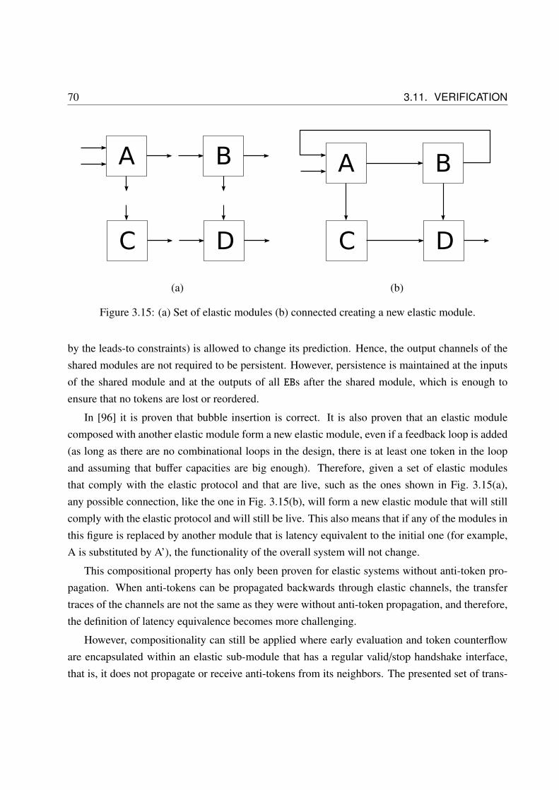
70 3.11. VERIFICATION
A B
C D
(a)
A B
C D
(b)
Figure 3.15: (a) Set of elastic modules (b) connected creating a new elastic module.
by the leads-to constraints) is allowed to change its prediction. Hence, the output channels of theshared modules are not required to be persistent. However, persistence is maintained at the inputsof the shared module and at the outputs of all EBs after the shared module, which is enough toensure that no tokens are lost or reordered.
In [96] it is proven that bubble insertion is correct. It is also proven that an elastic modulecomposed with another elastic module form a new elastic module, even if a feedback loop is added(as long as there are no combinational loops in the design, there is at least one token in the loopand assuming that buffer capacities are big enough). Therefore, given a set of elastic modulesthat comply with the elastic protocol and that are live, such as the ones shown in Fig. 3.15(a),any possible connection, like the one in Fig. 3.15(b), will form a new elastic module that will stillcomply with the elastic protocol and will still be live. This also means that if any of the modules inthis figure is replaced by another module that is latency equivalent to the initial one (for example,A is substituted by A’), the functionality of the overall system will not change.
This compositional property has only been proven for elastic systems without anti-token pro-pagation. When anti-tokens can be propagated backwards through elastic channels, the transfertraces of the channels are not the same as they were without anti-token propagation, and therefore,the definition of latency equivalence becomes more challenging.
However, compositionality can still be applied where early evaluation and token counterfloware encapsulated within an elastic sub-module that has a regular valid/stop handshake interface,that is, it does not propagate or receive anti-tokens from its neighbors. The presented set of trans-

CHAPTER 3. CORRECT-BY-CONSTRUCTION TRANSFORMATIONS 71
formations only use anti-tokens locally, and they very rarely need to traverse more than one or twolevels of elastic buffers. Therefore, such encapsulation is always possible within a small subgraphwhere model checking can be used to prove the correctness of the transformation. Then, the trans-formed subgraph can replace the original one and the global functionality of the design will notchange.
3.12 Conclusion
This chapter has presented a collection of correct-by-construction transformations which can beused to modify the microarchitecture of an elastic system. This way, it is possible to exploredifferent systems while it is guaranteed that functionality is preserved throughout the process.
Bypassing, retiming and multiplexor retiming are transformations valid for conventional se-quential circuits that have been adapted to elastic systems. The rest of the presented transforma-tions can modify the latency of the computations and hence, they can only be applied to latency-insensitive designs or to asynchronous designs. The verification of the presented transformationshas been discussed.

72 3.12. CONCLUSION

Chapter 4
Speculation
Speculation is a well-known technique for increasing parallelism of microprocessor pipelines andhence their performance. When the outcome of an operation is unknown during some cycle, but isrequired to perform another operation, two schemes can be considered for a correct behavior: (1)stall the pipeline until the first operation can provide the required data, or (2) predict the outcomeof the operation and continue the computations without stalling the pipeline. In the second case,the predicted result must be checked for correctness after the first operation has completed and,in case of misprediction, the speculated computations must be invalidated. If the predictions arehighly accurate, speculation may potentially provide a tangible performance improvement.
The most typical example of speculation is in the execution of branch instructions when thetarget address is predicted without knowing the outcome of the branch. If a misprediction is de-tected once the branch condition is calculated, the speculated instructions are invalidated and thecorrect flow is started.
Speculative execution can be introduced in elastic systems by applying a sequence correct-by-construction transformations, taking advantage of early-evaluation multiplexors and sharing offunctional units.
The contribution presented in this chapter is based on the results published in [64]. The intro-duction of this chapter provides an overview of the proposed method. A more thorough descriptionof the used transformations and the behavior of an speculative execution follows. Next, an opti-mization in elastic buffer implementation is presented, which allows to improve the throughputof speculative elastic systems by speeding up the transmission of critical anti-tokens. Finally, thebenefits of speculative execution in elastic systems are illustrated with two design examples.
73

74 4.1. INTRODUCTION
G
F0
1
(a)
G
F0
1
(b)
G
F 0
1F
(c)
G
0
1F
scheduler
(d)
Figure 4.1: Example of speculation in elastic systems: (a) non-speculative system, (b) system afterbubble insertion, (c) system after Shannon decomposition, (d) final design with speculation.
4.1 Introduction
The need for speculation arises when there is a decision point in the datapath in which some ofthe required data arrive late. Figure 4.1(a) shows a simple elastic circuit in which speculation canboost up its performance.
The loop through F and G could represent the computation needed to decide whether a branchinstruction is taken on a microprocessor. The two input channels would send the next ProgramCounter (PC) in case no branch is taken, and the next PC in case the branch is taken. Let usassume that there is a critical path starting at the EB, going through G, the multiplexor, F andarriving at the EB again. A possible way to optimize the performance of this design would be toinsert an empty EB in the critical path, as shown in Fig. 4.1(b). While this transformation wouldimprove the cycle time of the design, the throughput of the system would decrease to 1/2 becausethere is a loop with one token and two cycles of latency. The token would reach the multiplexoronce every two cycles, and during the other cycle there would be no real computation. Therefore,bubble insertion brings no real gain in this example. Retiming is not useful either. The number of
CHAPTER 4. SPECULATION 75
tokens in a loop is constant and cannot be changed.
Given a multiplexor with several inputs, it is possible to move a functional block from theoutput of the multiplexor to its inputs using Shannon decomposition [144] (viewed also as a mul-tiplexor retiming), as shown in Fig. 4.1(c).
After moving F from the output of the multiplexor to its inputs, F and G are executed in parallelrather than sequentially, achieving a better cycle time. Furthermore, the throughput of the systemis optimal as there are no bubbles. However, this speed-up comes at a price: duplication of logic.Here is where speculation can be effectively used. In order to reduce area, all copies of F can bemerged into a single one as shown in Fig. 4.1(d). Then, the system must speculate which inputchannel of the multiplexor should first use the shared functional module. The scheduler inside theshared module is the one that must select which input channel can propagate a token through theshared module, thus implicitly predicting the value of the select signal of the multiplexor.
When the speculation is correct, the early-evaluation multiplexor receives the required dataand computes its output. At the same time, an active anti-token is propagated backwards throughthe channel that was not selected, invalidating the unneeded data. When it is not correct, themultiplexor stalls. Then, the correct token must be propagated through F.
The design in Fig. 4.1(c) is optimal in performance. However, if the prediction strategy inFig. 4.1(d) is sufficiently accurate, the cycle clock penalty due to speculation will be rarely paid,achieving a similar performance with smaller power and area.
A manual implementation of all the stalling/canceling mechanisms for speculation is compli-cated and error-prone. A set of verified control primitives that can automatically take care of thesemechanisms in a distributed control fashion using local handshake protocols is highly useful. Fur-thermore, this control is introduced by applying provable correct-by-construction transformations,and hence functionality is preserved on the speculative design. Thus, an automatable and scalablescheme for speculation is provided.
4.2 Speculative Execution
As it has been explained in the previous section, speculation is introduced by applying the follow-ing steps:
1. Find critical cycles from the output of early-evaluation multiplexors to their select input. Ifsuch cycle exists, speculation is the transformation of choice for increasing the performance.
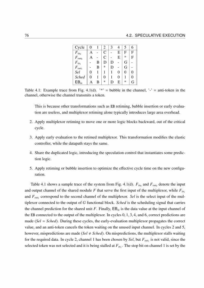
76 4.2. SPECULATIVE EXECUTION
Cycle 0 1 2 3 4 5 6Fin0 A - C - E F FFout0 A - C - E * FFin1 - B D D - G -Fout1 - B * D - G -Sel 0 1 1 1 0 0 0Sched 0 1 0 1 0 1 0EBin A B * D E * G
Table 4.1: Example trace from Fig. 4.1(d). ’*’ = bubble in the channel, ’-’ = anti-token in thechannel, otherwise the channel transmits a token.
This is because other transformations such as EB retiming, bubble insertion or early evalua-tion are useless, and multiplexor retiming alone typically introduces large area overhead.
2. Apply multiplexor retiming to move one or more logic blocks backward, out of the criticalcycle.
3. Apply early evaluation to the retimed multiplexor. This transformation modifies the elasticcontroller, while the datapath stays the same.
4. Share the duplicated logic, introducing the speculation control that instantiates some predic-tion logic.
5. Apply retiming or bubble insertion to optimize the effective cycle time on the new configu-ration.
Table 4.1 shows a sample trace of the system from Fig. 4.1(d). Fin0 and Fout0 denote the inputand output channel of the shared module F that serve the first input of the multiplexor, while Fin1
and Fout1 correspond to the second channel of the multiplexor. Sel is the select input of the mul-tiplexor connected to the output of G functional block. Sched is the scheduling signal that carriesthe channel prediction for the shared unit F. Finally, EBin is the data value at the input channel ofthe EB connected to the output of the multiplexor. In cycles 0, 1, 3, 4, and 6, correct predictions aremade (Sel = Sched). During these cycles, the early-evaluation multiplexor propagates the correctvalue, and an anti-token cancels the token waiting on the unused input channel. In cycles 2 and 5,however, mispredictions are made (Sel , Sched). On mispredictions, the multiplexor stalls waitingfor the required data. In cycle 2, channel 1 has been chosen by Sel, but Fout1 is not valid, since theselected token was not selected and it is being stalled at Fin1 . The stop bit on channel 1 is set by the

CHAPTER 4. SPECULATION 77
0
1F
scheduler
chan
nel 0
chan
nel 1
i i-1
i i-1in1
in0
out1
out0
Lf Lb
Figure 4.2: Example where the outcome of the early-evaluation multiplexor is predicted using theproposed method. Each one of the tokens is labeled with a counter (i or i − 1). The stage of EBsafter the shared unit has a forward latency of L f and a backward latency of Lb.
multiplexor, and this way the shared unit can realize a misprediction has been made. Then, Sched
is corrected during clock cycle 3.The performance gain obtained by applying speculation is based on the assumption that the
prediction can be done with a high probability of success. A good scheduler for a shared module isthe one that can foretell which channel from the available ones must be used. It is the designers jobto know how to take advantage of the circuit predictability. While the previous steps to introducespeculation are structural and can be easily automated, the design of a good scheduler may nottrivial or even not possible in some cases.
In order to illustrate how speculative execution using sharing units works, consider the examplein Fig. 4.2. There are two data channels sharing a functional module 1, and for simplicity ofexplanation, there is one EB at each input and one EB at each output of the shared module. Letus assume that the output EBs have forward latency L f and backward latency Lb. A special caseshown in the example in Fig. 4.1(d) (no buffers inserted) corresponds to the case of L f = 0 andLb = 0. Let us trace the processing of the i-th token, Ti, arriving at the input channel 0 of the sharedmodule. The processing goes through 3 steps:
Propagating to the input of the shared module. Since token order is always preserved in elasticsystems, for the i-th token, Ti, to be available at the input in0 of the shared module, the (i−1)-th token in this channel, Ti−1, must have been processed or canceled by an anti-token. Let usassume that the speculation controller of the shared module predicted channel 1 and hencedid not predict channel 0 during the previous transfer. Then, Ti−1 is stalled at in0, because itmay be used in case of misprediction. If prediction of channel 1 was correct, an anti-token
1This example can be easily generalized for sharing of k blocks

78 4.3. EBS WITH ZERO BACKWARD LATENCY
0
1F
scheduler
chan
nel 0
chan
nel 1
iin1
in0
out1
out0i
Lf Lb
Figure 4.3: Example from Fig. 4.2 once token i in channel 0 has been propagated to the input ofthe multiplexor.
is generated by the controller of the multiplexor into channel 0. This anti-token propagatesbackwards reaching in0 in Lb cycles and cancels Ti−1. Thus, the backward latency of EBscan affect the overall system performance and become a bottleneck. If the prediction waswrong, then the scheduler will have to let token Ti−1 use the sharing unit since it holds thedata required by the multiplexor for the (i − 1)-th data transfer.
Prediction by the scheduler of the shared module. Once token Ti arrives to the input of the sharedmodule, the scheduler may predict its channel and then Ti will get propagated through theshared module. Otherwise, the token Ti on channel 0 will be stalled until either the sched-uler changes its prediction during one of the future cycles or an anti-token generated by themultiplexor arrives and cancels it out.
Early evaluation in the multiplexor. After token Ti is selected by the scheduler, it is transmittedthrough the shared module and then, stored by the output EB. After L f cycles, the tokenreaches the input of the multiplexor, as shown in Fig. 4.3. If Ti was predicted correctly, oncethe select signal of the multiplexor becomes available, the early-evaluation multiplexor willgenerate a new token at its output. Otherwise, the token will be stalled at the input of themultiplexor, waiting for the correct token to arrive in the other channel.
4.3 EBs with Zero Backward Latency
As shown in the previous example, L f determines the latency needed by tokens to reach the inputof the multiplexor. In the multiplexor, the actual decision that was predicted takes place. Then, on

CHAPTER 4. SPECULATION 79
V+
in
V−
in
+
inS
−
inS
V+
out
V−
out
+
outS
−
outS
L = 1
L = 0f
b
EB Control
Din D
out
En
(a)
V+in
+in
S
V -in
-in
S
V +out
+out
S
V -out
-outS
En
V
R
(b)
Figure 4.4: (a) Datapath and (b) control for an elastic buffer with no backward latency.
correct predictions, anti-tokens are sent backwards to nullify the unneeded tokens waiting in theinput of the shared unit. This second latency is determined by Lb.
Anti-tokens must rush to the corresponding input channel of the shared module. Since theprediction was correct, the token at the input channel is no longer necessary. Each clock cycleelapsed since the multiplexor sends the anti-token until it reaches its final destination, the tokenwaiting at the input channel is causing a traffic jam, forcing next tokens to be stalled, potentiallyincreasing the queue size needed to store them and reducing the throughput.
Thus, it is possible to significantly improve the throughput of the elastic system by using EBswith Lb = 0 on the pipeline stages between the shared unit and the multiplexor making the deci-sions.
Figure 4.4(b) shows the control implementation for an EB with Lb = 0 and L f = 1. Theobjective of this controller is to propagate the V− bit as fast as possible. In order to maintain theintegrity of the protocol, the stop bit S + must also be sent combinationally. The S − and V+ bits arestored in a flip-flop and keep a forward latency of one clock cycle.
This controller is much simpler than the regular EB controller with Lb = 1 and L f = 1. However,its capacity is also smaller, it can only store one token (C = L f + Lb = 1). Since there is noneed to store two data items in the same EB at the same time, the datapath can be simplified andimplemented with a single flip-flop, as shown in Fig. 4.4(a), instead of using a pair of latches withindependent enable signals.
It can be verified that the controller in Fig. 4.4(b) complies with the SELF protocol and it isa refinement of the dual elastic buffer model discussed in Section 2.2.2. This implementation ofEB can be used to reduce the throughput overhead of speculation and in other paths where fast

80 4.4. DESIGN EXAMPLES
backward propagation is beneficial. However, a care must be taken not to chain too many of suchcontrollers to avoid potentially long combinational delays in the control, or even combinationalloops if they are connected forming a cycle.
4.4 Design Examples
So far, it has been assumed that speculation is used to improve the performance in a system whichis tightly constrained by a cycle going through the select signal of a multiplexor. In this case, somemodules can be removed from this cycle using Shannon decomposition and sharing. Then, thecritical cycle through the multiplexor becomes smaller and easier to optimize, thus improving theperformance of the system as long as it is possible to predict the behavior of the early-evaluationmultiplexor.
In this section, the use of speculation combined with elastic systems is demonstrated on two in-teresting examples. In these examples, there is no critical cycle going through an early-evaluationmultiplexor. However, speculation and early evaluation can still be used to improve their perfor-mance. First, a design with error detection and correction is presented. Speculation is used tostart the computation before the correctness of the input data is known. On the second example,speculation is used to propose an efficient implementation for variable-latency units.
For the experiments the actual datapath of the examples was designed in Verilog, connected tothe generated elastic controllers, and synthesized using commercial tools with a 65nm technologylibrary. The final designs were timed using STA and simulated in order to obtain the actual effectivecycle time.
4.4.1 Resilient Designs
Speculation can be used to add soft-error detection and correction in a pipeline without changingthe performance of the system in case of error-free behavior. The single error correction and doubleerror detection mechanism (SECDED) [153] is used as an example. For each 64 bits of data, 8 extrabits allow to detect and correct any single bit error. Besides, double bit errors are detected as well.Implementation details of SECDED can be found in [158].
Figure 4.5(a) shows an example with an adder where soft-error checking is done on each of itsinputs 2. Error correction needs a whole pipeline stage, and thus, the pipeline is deeper compared
2To simplify the figure, only one of the two inputs of the adder is drawn.

CHAPTER 4. SPECULATION 81
+0
1SECDEDerror
correcteddata
original data
(a)
+0
1SECDED
(b)
Figure 4.5: Speculation used for error correction and detection. (a) Original non-speculative re-silient system, (b) design after removing one pipeline stage.
to a design with no error checking. By adding speculation to the design, the computation can startwithout waiting for SECDED to finish. If errors are detected, then the corrected value producedby the error correction module can be used, spending an extra cycle. Thus, speculation enablesto achieve a shallower pipeline. This pipeline will probably have fewer data hazards, and hence itwill improve performance.
Since we know that the speculative design will not need a pipeline stage dedicated to errorcorrection, we can start by dropping this stage, as shown in Fig. 4.5(b). The EB that has beenremoved could have been retimed somewhere else or not even inserted initially. The cycle time inFig. 4.5(b) is larger than the one in Fig. 4.5(a), due to the path going through the error correctionunit plus the adder.
Next, Shannon decomposition can be applied to the adder to move it to the other side of themultiplexor. Since the error signal from the error detection unit going to the early-evaluationmultiplexor is critical in timing, it is better to retime the output EB and move the multiplexor to thenext pipeline stage. If possible, the select signal of early-evaluation multiplexors should not havea tight timing. Then, a bubble is added between the error correction unit and the adder, to breakthis long combinational path.transformed into a shared unit. The final design is shown in Fig. 4.6.
Since errors are expected to be unusual, the scheduler of the shared unit always predicts thatthe input data will be correct and the execution of the addition starts normally. At the same time,SECDED is computed on both inputs to detect errors in the input data. The bubble at the dataoutput of the error unit allows to store the corrected data in case of error. Next cycle, if SECDEDdetected an error, the mispredicted computation is stalled at the input of the multiplexor, and theaddition is restarted using the corrected values coming from the SECDED unit. Thus, the schedulermust only listen to the outcome of the SECDED unit to decide which decision to make. If there
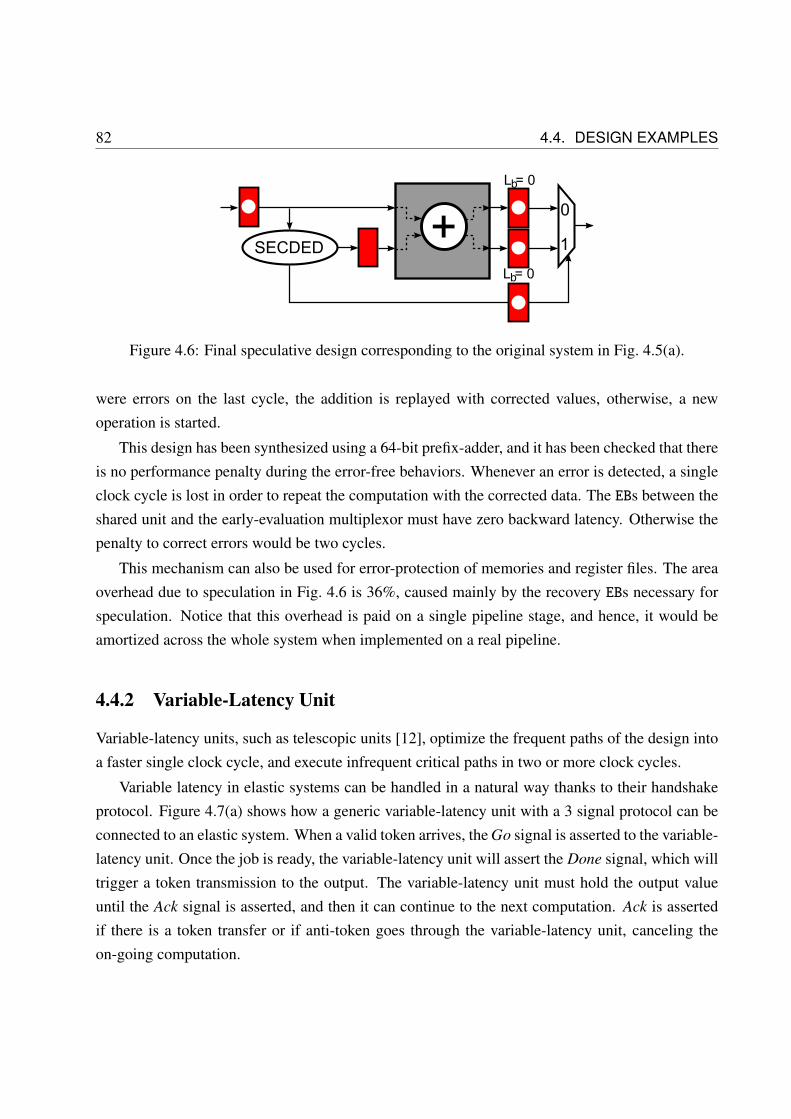
82 4.4. DESIGN EXAMPLES
0
1+L = 0b
SECDED
L = 0b
Figure 4.6: Final speculative design corresponding to the original system in Fig. 4.5(a).
were errors on the last cycle, the addition is replayed with corrected values, otherwise, a newoperation is started.
This design has been synthesized using a 64-bit prefix-adder, and it has been checked that thereis no performance penalty during the error-free behaviors. Whenever an error is detected, a singleclock cycle is lost in order to repeat the computation with the corrected data. The EBs between theshared unit and the early-evaluation multiplexor must have zero backward latency. Otherwise thepenalty to correct errors would be two cycles.
This mechanism can also be used for error-protection of memories and register files. The areaoverhead due to speculation in Fig. 4.6 is 36%, caused mainly by the recovery EBs necessary forspeculation. Notice that this overhead is paid on a single pipeline stage, and hence, it would beamortized across the whole system when implemented on a real pipeline.
4.4.2 Variable-Latency Unit
Variable-latency units, such as telescopic units [12], optimize the frequent paths of the design intoa faster single clock cycle, and execute infrequent critical paths in two or more clock cycles.
Variable latency in elastic systems can be handled in a natural way thanks to their handshakeprotocol. Figure 4.7(a) shows how a generic variable-latency unit with a 3 signal protocol can beconnected to an elastic system. When a valid token arrives, the Go signal is asserted to the variable-latency unit. Once the job is ready, the variable-latency unit will assert the Done signal, which willtrigger a token transmission to the output. The variable-latency unit must hold the output valueuntil the Ack signal is asserted, and then it can continue to the next computation. Ack is assertedif there is a token transfer or if anti-token goes through the variable-latency unit, canceling theon-going computation.

CHAPTER 4. SPECULATION 83
+S-
V
S-
V+
D
�� ��+
S-
V
S-
V+
DVariable-latency unit
Go Ack Done
(a)
0
+S
V+
-V
S-
+S-
V
S-
F
Fapprox
exact
G
DetectionError
Ferr
V+
DD
1
FF
FF
L
En
L
(b)
Figure 4.7: (a) Protocol to synchronize variable-latency units with elastic systems, (b) example ofa generic variable-latency unit which takes 1 or 2 clock cycles.
Figure 4.7(b) shows the datapath and control details for a variable-latency unit which can take1 or 2 clock cycles to compute. Fapprox is an approximation of Fexact that can be obtained automa-tically [9], and it has a shorter critical path. They can both be connected to the second part of thecomputation, called G in this example. Most of the computation cycles, the approximation is cor-rect (Fapprox = Fexact), and thus, Ferr = 0. Therefore, the function can be computed within a singleclock cycle, and the controller does not stall the token flow. However, when the approximation isincorrect, Ferr inserts a bubble into the receiver channel and stalls the sender. The next cycle Fexact
can be used to finish the computation. The communication between the datapath and the elasticcontroller is equivalent to the one in Fig. 4.7(a).
In Fig. 4.7(b), Ferr is connected directly to the controller, which handles the clock gatingmechanism to govern the datapath. The path from the V+ signal to the active low latches in-side the elastic buffer are shown in the figure. It is possible that Fexact followed by the comparisonto Fapprox plus the control gates until the latches become critical, specially if the datapath width is

84 4.5. CONCLUSION
0
1G
Fapprox
Fexact
Error?
L = 0b
Figure 4.8: Speculation used for variable latency.
large. Critical paths involving both datapath and control can be difficult to handle.
An alternative implementation that does not have this problem can be based on using specula-tion with replay in case of an error. The system in Fig. 4.8 always speculates that the approximatecomputation is always correct (in which case the computation is finished in one clock cycle). G
is shared between the channel coming from Fapprox and the channel coming from Fexact. On fastexecutions, the early-evaluation multiplexor selects the path coming from Fapprox, and a fast anti-token is sent through the EB with Lb = 0 in order to cancel the token from Fexact, which will bestored in the bubble. Whenever Ferr is asserted, the prediction was incorrect. Then, the next clockcycle, the speculation controller uses the result of Fexact computation stored in the bubble, whilethe early-evaluation multiplexor stalls waiting for the correct data. With this approach, the criticalpath is taken out of the elastic controller.
A variable-latency ALU has been implemented using a simple pipeline with an 8-bit datapath.In the initial system, shown in Fig. 4.7(b), Ferr is part of the critical path, going into the latchesof the control. This problem is gone in the final design shown in Fig. 4.8. The speculative designimproves the effective cycle time by 9% with a 12% area overhead. The area overhead is due toextra EBs storing the results after the shared unit. Furthermore, physical synthesis becomes simplerbecause the critical path does not end at a clock gating cell inside the controller.
4.5 Conclusion
This chapter has proposed a novel method for applying speculation in elastic systems, levera-ging the benefits of early evaluation and token counterflow. It is performed by applying Shannondecomposition and module sharing to a non-speculative design. Since both transformations arecorrect-by-construction, functional equivalence is preserved when applying speculation.

CHAPTER 4. SPECULATION 85
This method can provide a performance improvement on designs where the critical path lies in acycle that goes from the output of an early-evaluation multiplexor to its control signal. If this cycleis both critical in cycle time and in throughput, it may not be possible to improve the performanceby adding bubbles to further pipeline it. The proposed method allows to start execution of a partof the cycle speculatively, before it is known what of the input data will be selected by the early-evaluation multiplexor.
In order to do so, some logic blocks from the critical cycle are retimed out of the critical cycleto the input data of the multiplexor. These blocks are then shared by the elastic channels thatprovide data inputs to the critical early-evaluation multiplexor. A local scheduler decides which ofthe channels should be allowed to use the shared unit, trying to predict the selection of the early-evaluation multiplexor. The performance speed-up greatly depends on the quality of the scheduler.
It has been shown that speculation can be used to enhance performance of two realistic exam-ples. Speculation can be used to optimize variable-latency units, removing critical signals out ofthe control logic. Furthermore, it can be used to implement resilient designs that start performinguseful computation before the outcome of the error-checking unit is known, thus achieving a higherthroughput.

86 4.5. CONCLUSION

Chapter 5
Automatic Pipelining
In pipelined circuits, the structure and the boundaries of the pipeline is one of the most importantdecisions made early on the design process. This choice will have a direct impact on the per-formance and complexity of the final design. Furthermore, a poorly made decision may force aredesign later in the design process, with the corresponding increase in the cost of the circuit andpenalty in time to market. However, pipeline design is often done ad hoc, due to the significantcomputational costs of simulation during the design space exploration and the lack of analyticaloptimization methods capable of pipelining in the presence of dependencies between iterations.
Elastic systems provide many of the features required in order to implement efficient pipelines.The distributed handshake protocol controls data flow and can locally stall communications whensome data are not available. Early evaluation can be used to handle the control for the forwardingpaths, needed to maintain execution parallelism even in presence of data dependencies. Further-more, the set of elastic transformations presented in Chapter 3 provide a great set of tools for designoptimization.
This chapter presents a method that automates pipeline exploration using these transformations.The presented method combines mathematical models, such as retiming and recycling with earlyevaluation [24], with other heuristic methods. While manual crafting of an interlocked pipelinecan be laborious and error prone, this method guarantees a provably-correct construction becauseall the used transformations are correct-by-construction.
Design space exploration is driven by the expected workload for the circuit. Thus, the pipelineis optimized knowing which parts of the circuit will be executed more often and what is the ex-pected frequency for events such as data dependencies or instruction branches. This information
87

88 5.1. INTRODUCTION
W R
wa
rd
ra
wd F2F1
RF
(a)
W R
wa
rd
ra
wd
F2F1
=
0
1
(b)
W R
wa
rd
ra
wd
F2F1
=
0
1
(c)
W R
wa ra
wd
F2F1
=
0
1�
���
(d)
Figure 5.1: Simple pipelining example. (a) Initial functional specification, (b) design after applyingbypass to the register file, (c) retiming of the elastic buffer, and (d) bubble insertion in the bypasspath.
is very useful for optimization with elastic circuits, since it allows to adapt the latency of thecomputations and communications so that it is optimized to the expected workload.
The contributions presented in this chapter have been published in several conference andworkshop papers [48, 65, 66, 87]. This chapter first discusses how an unpipelined functional des-cription of a microarchitecture can be pipelined by applying a sequence of elastic transformations.Next, a method for automatic microarchitectural exploration is discussed and the efficacy of thisapproach is illustrated with some pipelining examples.
5.1 Introduction
Starting with a functional specification graph of a design, it is possible to pipeline it by using elastictransformations [87]. Bypasses with early-evaluation multiplexors are essential for pipelining,since they introduce new EBs that can be retimed backwards. In order to pipeline a design, bypassesmust be inserted around register files and memories of the functional model. Then, the graph ismodified to enable forwarding to the bypass multiplexors. Finally, the system can be pipelined byretiming the EBs inserted with the bypasses and using other transformations such as recycling oranti-token insertion. Speculation and insertion of variable-latency units can also be considered in

CHAPTER 5. AUTOMATIC PIPELINING 89
the exploration framework.Let us show how on the example in Fig. 5.1(a), which computes RF[wa] = F2(F1(RF[ra]))
at each clock cycle. Ignoring the delay of register reads and writes, the cycle period of the basicarchitecture (Fig. 5.1(a)) is determined by the sum of delays of F1 and F2. Let us assume that thetwo delays are equal (D), then the cycle time is 2D. The bypass transformation (explained in Sec-tion 3.4.1) incorporates new registers in the circuit and extra logic (multiplexor and comparison)to determine when the data must be read from the register file or from the bypass. By retimingthe new register, the circuit can be transformed from Fig. 5.1(b) to Fig. 5.1(c). Still, the period isdetermined by a critical path that starts at the input of F2 and ends at the output of F1 through thebypass. Assuming that the multiplexor delay is negligible, the cycle time is still 2D.
Here is where elasticity comes into play. A bubble can be inserted at one of the inputs of themultiplexor, as shown in Fig. 5.1(d). Now the cycle time is D. However, the bubble also has anegative impact on the performance. If early evaluation is not used, the throughput is determinedby the cycle containing two registers and one token. This results in processing only one data itemevery 2D time units. Hence the effective performance does not improve.
By using early evaluation, elastic pipelines attain optimal average-case performance by dynam-ically selecting bypasses using early enabling multiplexors. When no data hazards are present, themultiplexor propagates the data read from the register file and an anti-token is created in the bypasspath to kill the forwarded data, as shown in Fig. 5.2(a). However, when a bypass must be selected,the multiplexor cannot be enabled, and the system stalls waiting for the bypass data, as shown inFig. 5.2(b).
The exact throughput of the system (computed using Markov chains) is 1/(1 + α), where α isthe bypass probability (data hazard). Therefore, the speed-up of the pipelined microarchitecture is2/(1 + α). Figure 5.3 shows the relationship between the bypass probability and the speed-up inthis example.
5.2 Correct-by-construction Pipelining of a Simple Example
More complex transformations are often required in order to derive deeper pipelines. Figure 5.4(a)shows an example with two independent functions (M and ALU), each one with a different depth.The register file RF is the only state holding block. IFD fetches instructions and decodes theopcode and register addresses. The results are selected by the multiplexor for RF write-back. M
has been divided into three nodes. The breaking up of logic to allow pipelining is a design decision

90 5.2. CORRECT-BY-CONSTRUCTION PIPELINING OF A SIMPLE EXAMPLE
W R
wa
rd
ra
wd
F2F1
=
0
1-1
(a)
W R
wa
rd
ra
wd
F2F1
=
0
1
(b)
Figure 5.2: Simulation by case, (a) when bypass path is not needed, (b) when the register file isstalled waiting for a token in the bypass path.
1
1.2
1.4
1.6
1.8
2
0 0.4 0.6 0.8 1
Spee
d−up
Bypass Probability 0.2
Figure 5.3: Speed-up achieved by pipelining the example in Fig. 5.1(d) in function of the bypassprobability.

CHAPTER 5. AUTOMATIC PIPELINING 91
ALU
W R
wa
rd
ra
wd
M2 M3M1
IFDoc
RF
(a)
ALU
W R
wa
rd
ra
wd
M2 M3M1
IFD DDoc
(b)
ALU
W Rrdwd
M2 M3M1
oc
wa raIFD DD
(c)
ALU
W Rrdwd
M2 M3M1-1
-2
oc
wa raIFD DD
(d)
Figure 5.4: (a) Graph model of a simple design with two instructions, (b) After 3 bypasses, (c)Duplicate mux, enable forwarding, (d) Final pipeline after transformations.

92 5.3. EXPLORATION ENGINE
that is typically considered in concert with pipelining decisions. Thus, the user may try to divide afunctional block into several nodes and let the optimization algorithm decide the best channels toplace the EBs.
In Fig. 5.4(b), the bypass transform has been applied three times on RF to build a bypassnetwork. The node DD receives all previous write addresses and the current read address in orderto detect any dependencies and determine which of the inputs of the bypass multiplexor must beselected. The conventional use of bypasses is to forward data already computed to the read portof the bypassed memory element. In addition, this bypass network can be used as a data hazardcontroller, taking advantage of the underlying elastic handshake protocol with early evaluation tohandle stalls.
Notice that the EB closer to the register file cannot be retimed backwards in order to pipeline thedesign. One way to enable retiming of this EBwould be to apply anti-token insertion from Fig. 3.11on the dashed forwarding paths. However, adding an anti-token on the dashed path would stall thesystem every time there is a back to back data dependency, leading to a throughput degradation.
A better solution is to duplicate the WB multiplexor (the right-most one) and duplicate the by-pass EBs so that forwarding paths from the output of the functional units to the bypass multiplexorare created, as shown in Fig. 5.4(c) 1. Finally, by applying retiming and anti-token insertion trans-formations on Fig. 5.4(c), the pipeline in Fig. 5.4(d) can be achieved. The final elastic pipelineis optimal in the sense that its distributed elastic controller inserts the minimum number of stalls.Furthermore the pipeline structure is not redundant since there are no duplicated nodes. Therefore,this is as good as a manually designed pipeline.
Fast instructions, like ALU in this example, use the bypass network to forward data avoidingextra stalls, while long instructions use the bypass network as a stall structure that handles datahazards. In this example, the only possible stalls occur when the paths with anti-token countersare selected by the early-evaluation multiplexors. This situation corresponds to a read after write(RAW) dependency involving a result computed by M, which needs three cycles to complete.
5.3 Exploration Engine
The previous section shows how pipelining can be achieved by applying transformations one byone. For a given elastic system, there are many different possible pipelines. For example, Fig. 5.5
1See Section 5.3.2 for an example which shows why forwarding paths are needed

CHAPTER 5. AUTOMATIC PIPELINING 93
ALU
W Rrdwd
M2 M3M1-1
oc
wa raIFD DD
Figure 5.5: Another possible pipeline for the graph in Fig. 5.4(a).
shows an alternative pipeline for the design in Fig. 5.4(a). In this example, only two bypasses havebeen applied to the register file. Then, in order to fully pipeline M operation, a bubble is used inthe final stage.
At first sight, it is difficult for a human to determine whether Fig. 5.5 is better than Fig. 5.4(d).Figure 5.5 provides the same cycle time or slightly better (since there are fewer bypasses and hencefewer multiplexors) than Fig. 5.4(d) and a smaller area (there are fewer EBs). However, the cyclesgoing through M have a worse token/delay ratio in Fig. 5.5, and hence a worse throughput. Theeffective cycle time of Fig. 5.5 will be better when M is rarely used, but it will be worse if it is usedtoo often.
A designer performing manual exploration may miss some of these configurations with betterperformance or a more interesting performance/area trade-off. Furthermore, manual explorationis tedious and it becomes harder as the microarchitectural graph grows. Pipelining a system withhundreds of nodes manually is close to impossible.
An algorithm that automatically explores the design space can potentially find better designs, orat least, provide better confidence on the value of the solution. This section proposes an automaticexploration framework. First, the retiming and recycling optimization is presented. Retimingand recycling is used in the inner loop of the proposed method. Then, it is shown how to addbypasses and forwarding paths to microarchitectural graphs. Finally, the exploration methodologyis discussed and an exploration algorithm is proposed.

94 5.3. EXPLORATION ENGINE
5.3.1 Retiming and Recycling
This section reviews the retiming and recycling (RR) problem [24], which is used by the innerloop of the method presented in this chapter. RR formalizes a subset of the elastic transformationspresented in Chapter 3 (early evaluation, retiming of EBs, insertion of empty EBs, insertion andretiming of anti-tokens) and solves an optimization problem on this formalization in order to findthe configuration with the best effective cycle time. This problem was initially proposed in [35] andsolved as a mixed integer linear programming problem (MILP) in [26]. Finally, it was extended tosupport early evaluation and anti-tokens in [24].
Given a microarchitectural graph G(N, E) and an initial number of tokens on each edge definedby a vector R0 ∈ Z
|E|, a retiming and recycling configuration, RC, is a pair of vectors R′0 ∈ Z|E|,
R′ ∈ Z+ |E|, where R′0 assigns a number of tokens to each edge and R′ assigns a number of EBsto each edge. For each edge e, there must be enough EBs to store all tokens in the edge, i.e.,R′(e) ≥ R′0(e). R0 and R′0 can be negative, which represents anti-tokens. The capacity of all EBs isassumed to be large enough. Furthermore, each node n is assigned a combinational delay δ(n) anda latency lat(n).
A retiming vector r ∈ Z|N|, is a map N → Z that for every edge e = (u, v) transforms R0 to R′0as follows: R′0(e) = R0(e) + r(v) − r(u). Thus, r(u) indicates how many tokens (or anti-tokens) areretimed through node u and in which direction.
Some elastic transformations presented in Chapter 3 can be represented on an RC using a re-timing vector r. Bubble insertion on edge e can be achieved by incrementing R′(e). Given twoedges e0 = (u, v), e1 = (v, z) such that R0(e1) = 0, anti-token insertion is represented by r(v) = 1:this adds one token to e0 and inserts one anti-token to e1. This new token inserted on e0 withanti-token insertion transform can be then retimed through node u. Backward retiming of tokensis achieved by incrementing r(v), and forward retiming by decrementing r(v). Analogously, back-ward retiming of anti-tokens is achieved by decrementing r(v) and forward retiming of anti-tokensis achieved by incrementing r(u). Thus, insertion, retiming and grouping of anti-tokens can alsobe easily modeled using retiming vectors.
Finally, the cycle time of the system, τ, can be constrained using a set of linear equations calledPath_Constr(RC, τ), and the inverse of the throughput, x = 1/Θ, can also be constrained using aset of linear equations called Thr_Constr(RC, x). These sets of equations are defined in [23, 24].Finally, the function to optimize is the effective cycle time ξ = τ/Θ = τ × x. The final problem to

CHAPTER 5. AUTOMATIC PIPELINING 95
solve is :Minimize x · τ,
R′0(e) = R0(e) + r(v) − r(u),R′ ≥ R0,R′ ≥ 0,Path_Constr(RC, τ),Thr_Constr(RC, x),
(5.1)
Since Thr_Constr(RC, x) is an upper bound approximation of the throughput, the exact solu-tion of Equation (5.1) is not necessarily the one with the minimum effective cycle time, but it istypically a very good approximation. On the other hand, Equation (5.1) represents a big challengefor existing solvers, since the objective function is not convex. A faster heuristic method based onmixed integer linear programming is presented in [24]. Given two RCs, RC1 and RC2, RC1 dominatesRC2 if Θ(RC1) > Θ(RC2) and τ(RC1) ≤ τ(RC2).
The heuristic method to solve Equation 5.1 finds the set of non-dominated RCs. Each RC canbe considered a Pareto point which explores a different cycle time / throughput trade-off2. The firstPareto point found by the heuristic has the minimum possible cycle time, equal to the maximumnode delay. Then, each Pareto point has a larger cycle time, and also a larger throughput. The lastpoint corresponds to the min-delay retiming configuration, which has no bubbles and always hasthroughput equal to 1.
For example, Fig. 5.6 shows an example that has three non-dominated Pareto-point configura-tions. The first Pareto point is the optimal one, since its effective cycle time is 2, compared to 3 forthe other two configurations. If the early-evaluation multiplexor had different probabilities at theinputs, the configurations may be different, or they may be the same but the optimal one in termsof effective cycle time could be a different one.
5.3.2 Bypassing and Forwarding
Figure 5.7(a) shows a register file with 3 bypasses. Write address and read address are omittedfor simplicity. Even though three EBs have been inserted, only the leftmost one can be retimedbackwards. Bypasses alone are not sufficient to pipeline cyclic systems.
By using the anti-token insertion multiple times, EBs and anti-tokens can be inserted on the by-pass channel. Then, all the EBs can be retimed out of the bypass structure, as shown in Fig. 5.7(b),and used to pipeline the design along the dotted line. However, the inserted anti-tokens will stall
2Strictly speaking Pareto points are formed by the pairs (Θ(RC),−τ(RC))

96 5.3. EXPLORATION ENGINE
100.5 11 0.5
-2
(a)
100.5 11 0.5
-1
(b)
100.5 11 0.5
(c)
Figure 5.6: Example with three non-dominated Pareto-point configurations found by retiming andrecycling. Their performance metrics are (a) τ = 1,Θ = 0.5, ξ = 2, (b) τ = 2,Θ = 0.66, ξ = 3, (c)τ = 3,Θ = 1, ξ = 3.
W Rrd
wd p
p
p
p
3
2
1
(a)
W Rrd
wd p
p
p
p
3
2
1
-2-1
(b)
Figure 5.7: 3 bypasses (a) before retiming, (b) after retiming using anti-tokens.
the system on data hazards, waiting for the correct token to arrive.
Data hazards can also be solved by forwarding the required value if it is already availablesomewhere within the pipeline. In order to enable forwarding to the bypass multiplexor, some EBsand multiplexors must be duplicated to create new paths.
For example, after bypassing the register file three times in the graph in Fig. 5.4(b), some nodesin the graph are duplicated to achieve the system in Fig. 5.4(c). In this figure, each bypass is fed in-
ALU
W R
M2M1-1
IFD DD
(a)
ALU
W R
M2M1 -1
IFD DD
(b)
Figure 5.8: Example pipeline (a) without using forwarding paths, (b) using forwarding paths.

CHAPTER 5. AUTOMATIC PIPELINING 97
dependently, creating new forwarding paths and retiming opportunities that can lead to the retimeddesign in Fig. 5.4(d). In order to automatically create all the possible forwarding paths so that theycan be used by RR optimization, it is necessary to traverse the microarchitectural graph backwardsstarting from the register file, and duplicate all the fork nodes, with the corresponding buffers, untilthe write-back multiplexor is found. The write-back multiplexor should also be duplicated. Thesefork nodes are drawn as small points in Fig. 5.7(a).
Figure 5.8(a) shows an example similar to the one in Fig. 5.4, but the M execution unit has only2 stages instead of 1 (to make it simpler). In this example, no forwarding paths have been added.The pipelining has been built just by applying anti-token insertion and retiming. Figure 5.8(b)shows the same example where the forwarding paths have been added. In both figures, the cyclethat corresponds to a back-to-back dependency between consecutive ALU instructions has beenhighlighted. In the example with forwarding paths, this cycle has a throughput of 1. However, inthe example without forwarding paths, this cycle has a throughput of 0.5, since it has 1 token (2tokens and 1 anti-token) and two EBs. Therefore, the example with forwarding paths will have ahigher throughput as long as this cycle does not have 0 probability.
Furthermore, it is not possible to achieve a throughput of 1 for this cycle without adding thecorresponding forwarding path. It is the only way to provide the data produced by the ALU assoon as possible. Using the same write-back multiplexor that provides data to the register filemeans delaying the data transmission, with the corresponding performance penalty. After runningthe retiming and recycling optimization, some of the fork nodes and early-evaluation multiplexorscreated in order to enable some forwarding paths may be merged back if they have not been fullyused (e.g., the three write-back multiplexors in Fig. 5.4(c) could be merged back since they havethe same inputs with the same exact latency).
In order to be able to analyze the performance of a microarchitectural graph without simulating,it is necessary to assign probabilities to the inputs of early-evaluation multiplexors. For bypassstructures, these probabilities should be determined by the expected frequencies of data hazards inthe class of workloads for which optimization is done.
In this work, data hazard probability is modeled on bypass multiplexors with a single probabil-ity, γ, which represents the probability that the register file reads the value written at the previousclock cycle (back-to-back dependency). Then, further dependencies are assumed to decrease ge-ometrically. Thus, the probability of p1 (from Fig. 5.7(a)) to be selected by the multiplexor isp(p1) = γ; the probability that the register file reads the data value written two clock cycles before,i.e., distance two dependency, is p(p2) = (1 − γ)γ; and in general, the probability of distance i

98 5.3. EXPLORATION ENGINE
Simulate
performance
Obtain actual
Set of
near-optimal
designs
Yes No
Add bypass toone or more
memory elements
R&R MILPmethod
Initial Graph
Improve?
Figure 5.9: High level view of the exploration algorithm.
dependency is p(pi) = (1 − γ)i−1γ. The path from the register file directly to the multiplexor (nodependencies) is taken when no other path is selected.
5.3.3 Two-phase Exploration
Simulations of Verilog controllers can take significant time: up to 30 minutes for a several hundredsnode example and 10K simulation cycles. Thus, it is not feasible to simulate each of the RCs foundby RR executions, because the exploration time would become too large.
Depending on the number of early-evaluation nodes and the number of cycles in a graph, eachRR execution may find up to 7 or 8 different Pareto points. For example, if there are two elementsthat can be bypassed, and the algorithm tries up to 11 bypasses to each one, there can be close toa thousand of different configurations. In order to prune the design space, bypasses are appliedgreedily instead of trying all combinations, and the throughput is estimated rather than simulatedduring the first stage of the exploration.
Hence, design space is explored using a two-phase exploration strategy, similar to [62]. Duringthe first phase, bypasses are applied incrementally on the memory elements and RR optimizationexecuted on each step, as shown in Fig. 5.9. Within RR, performance for each point is estimatedusing analytical analysis, and the most promising points are stored. At the end of the exploration,each of the design points with near-optimal performance is simulated in order to determine their

CHAPTER 5. AUTOMATIC PIPELINING 99
throughput with better accuracy. Finally, the method returns the configuration with the best effec-tive cycle time or a set of Pareto-point configurations with different effective cycle time and area.
Since the ordering determined by throughput analysis and by simulation are similar (see Sec-tion 6.5.2), it can be safely assumed that design points pruned during the first phase are not optimal.
5.3.4 Exploration Algorithm
During the exploration phase, Algorithm 1 tries different number of bypasses for each of the mem-ory nodes of the graph. Even though the number of elements in a microarchitecture that can bebypassed is not typically large, it is interesting to be able to support an undetermined numberof them. If there is a single register file, the algorithm adds one bypass at each iteration, addsthe corresponding forwarding paths and then calls the retiming and recycling function (RR) forperformance optimization.
The more bypasses the algorithm adds, the less recycling is needed for achieving a small cycletime through pipelining. Therefore, the throughput (and the effective cycle time) keeps improvingat each iteration, while the cycle times can be kept constant. At some point, either the number ofbypasses is enough to fully pipeline the design using retiming, or the throughput degradation due todata hazards stalls in the new bypass is larger than the cycle time improvement due to pipelining.At this point, adding more bypasses does not improve the performance, and the exploration iscompleted.
If the graph has several memory elements, the exploration can be performed in a similar way,but the algorithm selects which element to bypass next based on sensitivity analysis. Given agraph G with a set of elements that can be bypassed (memories(G)), Algorithm 1 greedily selectswhich element to bypass. For every memory m, H.bypass(m) applies one more bypass and addsthe corresponding forwarding paths. Then, the algorithm calls RR optimization and estimates theeffective cycle time (ξlp(c)) for each Pareto point c found by RR.
The node m that leads to the fastest configuration is chosen as the next step, and the greedyalgorithm continues into the next iteration. Variable ξloop keeps track of the best effective cycletime and Gloop stores the best graph found so far within the loop of the algorithm.
When the estimated effective cycle time cannot be improved with a given threshold (calledimprove_threshold in the algorithm), the exploration stops. The priority queue explored_points
stores the best designs within a given performance overhead compared to the best design found byanalytical estimation. At the end, all stored designs are simulated in order to find the best one. In

100 5.3. EXPLORATION ENGINE
Algorithm 1: Bypass_One(G).explored_points := ∅ #Set to keep the most promising design pointsξmin := ∞ #Best effective cycle time founddone := false #Boolean to indicate when exploration is overwhile not done do
ξloop := ξ0 := ξmin #Best effective cycle time within the loopfor m ∈ memories(G) do
H := GH.bypass(m) #Adds one bypass plus forwarding paths to memory mRCs := RR(H) #Returns all the Pareto-point configurations foundfor c ∈ RCs do
explored_points.add(c) #Store the design point if it is promisingξmin := min(ξlp(c), ξmin)if ξlp(c) < ξloop then
#New best configuration found within the loopGloop := Hξloop := ξlp(c)
done := ξmin ≥ ξ0 ∗ (1 − improve_threshold)G := Gloop #Recover best configuration for next iteration
return G, explored_points
addition to the best design point, with effective cycle time ξmin, the frontier of best solutions is kept,because the analytical LP formulation for the effective cycle analysis is approximate. Therefore,some other points in the frontier close to the best estimated may have the best performance (as canbe checked by simulation). The ability to store a set of solutions can be also used to extend thealgorithm for generating Pareto points in the (performance, area) solution space.
Some graphs may require several memory elements to be bypassed at the same time in orderto reach a performance improvement. On such designs, the previous algorithm may be inefficient.Therefore, Algorithm 2, which bypasses all memory nodes at the same time before RR is called,is executed first. After a local minimum is found by Algorithm 2, Algorithm 1 is called for finergrain tuning.
If a memory node is not further bypassed by the Algorithm 1, it might have too many bypasses.For example, say a graph has two memory elements and the optimal configuration has 3 bypassesfor the first memory and 9 for the second. Assume that Algorithm 2 bypasses the graph until(7,7), and then Algorithm 1 continues until (7,9). Extra bypasses do not degrade the performanceof the system, since the same pipelining can be achieved for (7,9) and for (3,9). Configuration

CHAPTER 5. AUTOMATIC PIPELINING 101
Algorithm 2: Bypass_All(G).explored_points := ∅ξmin := ∞done := falsewhile not done do
ξ0 := ξmin
for m ∈ memories(G) doG.bypass(m)
RCs := RR(G)for c ∈ RCs do
explored_points.add(c)ξmin := min(ξlp(c), ξmin)
done := ξmin ≥ ξ0 ∗ (1 − improve_threshold)return G, explored_points
(7,9) contains unnecessary bypasses. By running Algorithm 1 again starting from the best designfound, (7,9), but using unbypass transformation instead of bypass, the design space can be furtherexplored. Algorithm 1 with unbypass has a different termination condition: instead of checkingthat a better design point is found, it checks that the best RR Pareto point is not significantly worsethan the best ξ found so far.
Algorithm 3: Top-level Exploration Algorithm.Gbest, explored_points1 := Bypass_All(G)Gbest, explored_points2 := Bypass_One(Gbest)Gbest := simulate(explored_points1 + explored_points2)H, explored_points := Unbypass_One(Gbest)Gbest2 := simulate(explored_points)
The top-level algorithm, shown in Algorithm 3, calls Algorithm Bypass_All first and thenAlgorithm Bypass_One. Next, the best design points are simulated in order to obtain the best onefrom this first exploration. Since it may be over-bypassed, Algorithm Bypass_One with unbypasstransformation is called, to further explore new design points. At the end, this new explored pointsare simulated. The performance of Gbest2 can be at most equal to Gbest. It has not been observed alarge performance difference between them in any of the experiments. Depending on the area gainand the performance loss of Gbest2 , the user can decide which one to take as the best one.
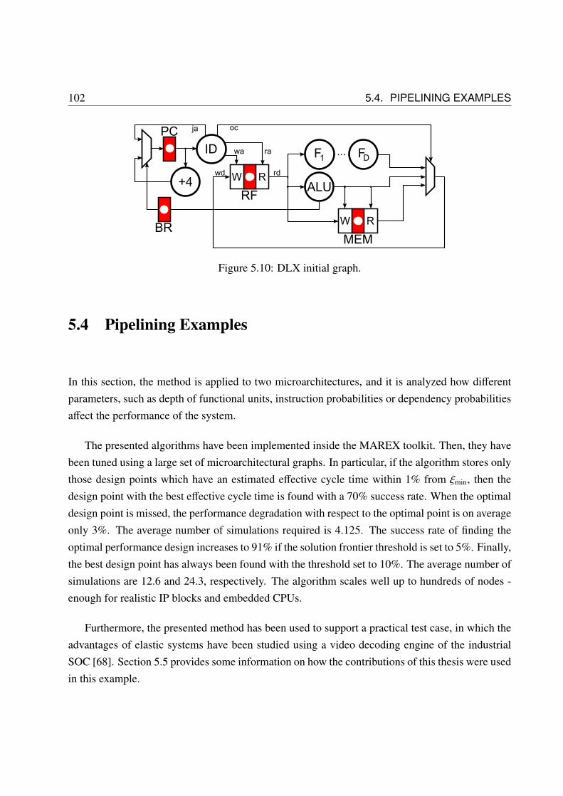
102 5.4. PIPELINING EXAMPLES
W R
ID
RFALU
W R
MEM
PC
F
+4rdwd
wa ra
ocja
BR
1 FD...
Figure 5.10: DLX initial graph.
5.4 Pipelining Examples
In this section, the method is applied to two microarchitectures, and it is analyzed how differentparameters, such as depth of functional units, instruction probabilities or dependency probabilitiesaffect the performance of the system.
The presented algorithms have been implemented inside the MAREX toolkit. Then, they havebeen tuned using a large set of microarchitectural graphs. In particular, if the algorithm stores onlythose design points which have an estimated effective cycle time within 1% from ξmin, then thedesign point with the best effective cycle time is found with a 70% success rate. When the optimaldesign point is missed, the performance degradation with respect to the optimal point is on averageonly 3%. The average number of simulations required is 4.125. The success rate of finding theoptimal performance design increases to 91% if the solution frontier threshold is set to 5%. Finally,the best design point has always been found with the threshold set to 10%. The average number ofsimulations are 12.6 and 24.3, respectively. The algorithm scales well up to hundreds of nodes -enough for realistic IP blocks and embedded CPUs.
Furthermore, the presented method has been used to support a practical test case, in which theadvantages of elastic systems have been studied using a video decoding engine of the industrialSOC [68]. Section 5.5 provides some information on how the contributions of this thesis were usedin this example.

CHAPTER 5. AUTOMATIC PIPELINING 103
Block Delay Area Lat. Block Delay Area Lat.mux2 1.5 1.5 1 EB 3.15 4.5 1ID 6.0 72 1 +4 3.75 24 1ALU 13.0 1600 1 F 80.0 8000 1RF W 6 6000 1 RF R 11 - 1MEM W - - 1 MEM R - - 10
Table 5.1: Delay and area numbers for DLX example using NAND2 with FO3 as unit delay andunit area.
5.4.1 DLX pipeline
This method is first illustrated on a simple microarchitecture similar to a DLX, shown in Fig. 5.10before pipelining. The execution part of the pipeline has an integer ALU and a long operationF. The instruction decoder ID produces the opcode, oc, that goes to the write-back multiplexorand a target instruction address, ja, that is taken in function of the previous ALU operation, asstored in the register BR. Table 5.1 shows approximate delays, latency and area of the functionalblocks of the example, taking NAND2 with FO3 as unit delay and unit area. In order to obtainthese parameters, some of the blocks have been synthesized in a 65nm technology library usingcommercial tools (ALU, RF, mux2, EB and +4), and the rest of the values have been estimated.EB and mux2 delay and area numbers were taken for single bit units. The delay of bit-vectormultiplexors and EBs is assumed to be the one shown in the table, while area is scaled linearlyw.r.t. the number of bits. Multiplexors with a fan-in larger than two are assumed to be formed bya tree of 2-input multiplexors.
Even though a conventional DLX pipeline does not typically include this feature, F is consid-ered to be a floating point unit. Its total delay is set to 80, around 5 times the expected cycle timeof the design. Then, it may be partitioned in several stages (F1, F2, . . . FD) to allow pipelining. Itis assumed that the delay of each stage is 80/D. Notice that partitioning of F must be provided bythe designer a priori, it is not performed automatically by the exploration algorithm. However, itis possible to provide several possible partitionings and perform design exploration on each one,thus determining the optimal pipeline depth.
The register file is 64 bits wide, with 16 entries, 1 write and 2 read ports. The total footprintof the RF is 6000 units, (including both cell and wire area). To account for wiring of other blocks,we assume that 40% space is reserved for their wiring. Furthermore, we also need to consider thearea overhead of elastic controllers. Based on experiments with multiple design points, a 5% area
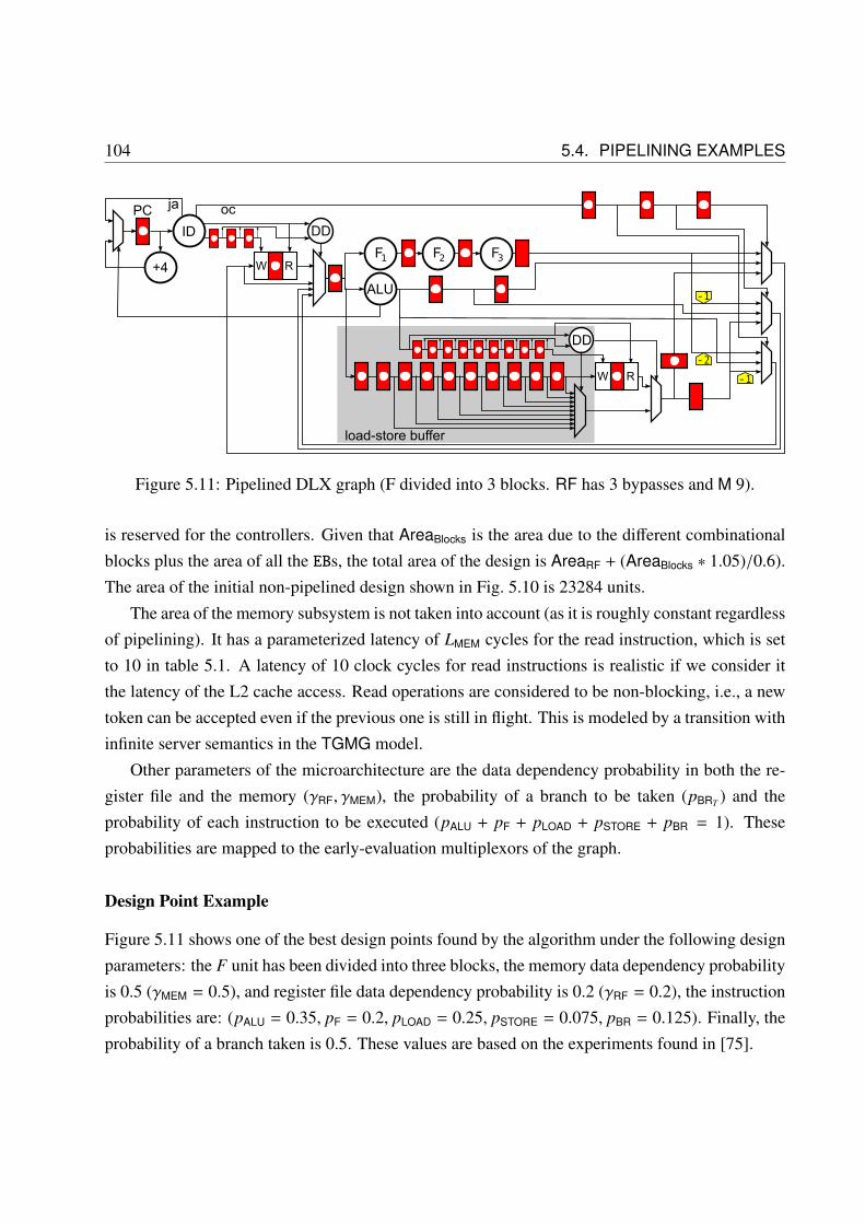
104 5.4. PIPELINING EXAMPLES
ID
ALU
PC
+4
ocja
-1
-2
W R
DD
W R
DD
load-store buffer
-1
F1 F2 F3
Figure 5.11: Pipelined DLX graph (F divided into 3 blocks. RF has 3 bypasses and M 9).
is reserved for the controllers. Given that AreaBlocks is the area due to the different combinationalblocks plus the area of all the EBs, the total area of the design is AreaRF + (AreaBlocks ∗ 1.05)/0.6).The area of the initial non-pipelined design shown in Fig. 5.10 is 23284 units.
The area of the memory subsystem is not taken into account (as it is roughly constant regardlessof pipelining). It has a parameterized latency of LMEM cycles for the read instruction, which is setto 10 in table 5.1. A latency of 10 clock cycles for read instructions is realistic if we consider itthe latency of the L2 cache access. Read operations are considered to be non-blocking, i.e., a newtoken can be accepted even if the previous one is still in flight. This is modeled by a transition withinfinite server semantics in the TGMG model.
Other parameters of the microarchitecture are the data dependency probability in both the re-gister file and the memory (γRF, γMEM), the probability of a branch to be taken (pBRT ) and theprobability of each instruction to be executed (pALU + pF + pLOAD + pSTORE + pBR = 1). Theseprobabilities are mapped to the early-evaluation multiplexors of the graph.
Design Point Example
Figure 5.11 shows one of the best design points found by the algorithm under the following designparameters: the F unit has been divided into three blocks, the memory data dependency probabilityis 0.5 (γMEM = 0.5), and register file data dependency probability is 0.2 (γRF = 0.2), the instructionprobabilities are: (pALU = 0.35, pF = 0.2, pLOAD = 0.25, pSTORE = 0.075, pBR = 0.125). Finally, theprobability of a branch taken is 0.5. These values are based on the experiments found in [75].

CHAPTER 5. AUTOMATIC PIPELINING 105
Figure 5.12: Effective cycle time and area of the best pipelined design for different depths of F.(x,y) and (x,y,z) tuples represent the depth of F, the number of bypasses applied to RF and to MEM(z = 9 if omitted).
In Fig. 5.11, the cycle time is 29.817 time units, due to the F1, F2 and F3 functional blocks.3 bypasses have been applied to RF and then EBs have been retimed to pipeline F. Note that thealgorithm inserted an extra bubble at the output of F3: the reduction in the throughput due to thisbubble, is compensated by a larger improvement in the cycle time (without this bubble the criticalpath would include the delay of the multiplexors after F3). If F operation had a higher probability,the design without this bubble might be better, since the bubble would have a higher impact on thethroughput degradation. Such decisions are made automatically based on the expected frequenciesof instructions and data dependencies. An alternative way to avoid the bubble after F3 is to addan extra bypass to RF. An extra bypass is indeed the optimal way to pipeline the design for thisparticular instance of the parameters. It may not be the case if the data hazard probability washigher.

106 5.4. PIPELINING EXAMPLES
Optimal Depth
Figure 5.12 shows the effective cycle time and area of the best design point found by the presentedmethod on different depths of F, forming a Pareto-point curve. The first point on the x scalecorresponds to a graph where F is a single node, the second one corresponds to a graph where F ispartitioned into F1,F2, etc. The parameter values are the same ones as in Fig. 5.11. The delay ofF is the largest one, and as the number of nodes in which it is partitioned increases, the maximumnode delay decreases, and so does the best possible cycle time in the graph. In the best design forthe graph in which F is not partitioned (depth(F) = 1), the effective cycle time is 87.99, the area is32791, 2 bypasses have been applied to RF and 8 bypasses have been applied to MEM. The cycletime of this first point is 83.15 (δ(F) + δ(EB)), and the throughput is 0.94. Only back-to-back datadependencies involving F instructions require stalling of the pipeline.
As depth(F) increases, more bypasses are applied to the register file. The area of the designincreases with more bypasses. For depth(F) = 2, the cycle time is 43.15, the throughput is 0.86and the effective cycle time is 49.77. Until depth(F) = 6, the cycle time keeps decreasing becauseof the deeper pipeline (43.15, 29.81, 23.15, 19.26, 16.48), and so does the throughput because moredata hazards must be handled. Overall, the effective cycle time improves with a deeper pipelineuntil 6 stages are reached.
For depth(F) = 7, the delay of each stage of F becomes lower than the delay of the ALU
(δ(Fi) = 80/7 = 11.4). Thus, the cycle time cannot be further improved by increasing the depth ofF. Thus, the best effective cycle time is achieved with F divided into 6 stages, 8 bypasses appliedto RF and 9 to MEM. Design points (4,5) and (3,4) (circled in the figure) for 4 and 3 stages aresimpler and overall might deliver a better design compromise.
Different parameters lead to different optimal design points. For example, when γRF = 0.5,bypass paths are selected more often and the throughput is generally worse, since more stalling isneeded. However, in this case the optimal depth of F becomes 7 instead of 6. Different instruc-tion probabilities also lead to different optimal design points. If the microarchitecture issues ALU
instructions most of the time, the throughput is close to 1 on the designs, since data dependenciescan always use forwarding in order to avoid stalls. Besides, since F operations are never selected,less bypasses are applied and recycling is used in order to pipeline F. Because of the store bufferadded by bypasses on MEM, memory operations can also be performed with a high throughput.On the other hand, if F instructions are the most common ones, the throughput degrades faster asthis instruction always needs to stall the pipeline when a data dependency occurs.

CHAPTER 5. AUTOMATIC PIPELINING 107
Figure 5.13: Throughput of the memory subsystem given different read latencies and bypass de-pendency probability. In the legend, l_x_p_y, means LMEM = x, γMEM = y.
The time needed to run algorithm 3 is usually around 200 seconds for every DLX configuration.The longest exploration took 400 seconds. Parameters such as F depth or memory latency havean impact on the run-time, since more bypasses need to be applied. Most of the exploration time,around 93%, is spent solving RR ILP problems using the CPLEX solver [55]. Simulation timedepends on the number of near-optimal points found by the algorithm. If the threshold is set to 1%,the average number of simulations is 4.125, and the average simulation time is 150 seconds. Higherthresholds provide more variety of possible designs but require more time in order to simulate allof them.
Memory subsystem
Bypasses done on RF are useful because the inserted EBs are retimed to pipeline F. On the otherhand, memory bypasses are used to hide the memory latency via a load-store buffer, as shown inFig. 5.11. When a read operation starts, if the address being read has been written during the last9 clock cycles, the early-evaluation multiplexor can get the token from the store buffer withoutwaiting for the read operation. Otherwise, the multiplexor stalls the execution until the token from

108 5.4. PIPELINING EXAMPLES
W R F
W R F
W R F
�
���0
0
�
���1
1
�
���2
22
1
0
Figure 5.14: Ring of pipelines.
the memory arrives. Such structure can be substituted by a more efficient implementation: anassociative memory. The algorithm automatically detects the need for a load-store buffer and itsoptimal size.
Figure 5.13 shows the throughput of the memory subsystem given different latencies of mem-ory reads and different dependency probabilities. The x-axis is the number of bypasses applied. Itcan be seen that the lines in the figure that have the same bypass probability γMEM have the sameshape, shifted to the right as the latency is larger. Lower memory latencies, larger number of by-passes and larger dependency probabilities affect the throughput positively. If data dependenciesare rare, it is not possible to reach a throughput close to 1. Also notice that for the parameters usedon the previous experiment (LMEM = 10, γMEM = 0.5), 9 bypasses give an optimal throughput.
5.4.2 Ring of pipelines
In order to further discuss this method and the implication of different microarchitectural parame-ters on the performance, a simple parameterized microarchitecture is used in this section.
This microarchitecture is formed by k pipelines, each one consisting of a functional unit Fi anda register file Ri, where 0 ≤ i < k. Each register file Ri receives the output of Fi with probability αi,otherwise it receives the output of register file R(i−1) mod k, forming a ring of pipelines. Figure 5.14shows the microarchitecture for k = 3.
Each register file has a bypass probability γi, and each functional unit has a delay δ(Fi). Fi hasa depth di, and hence it is split into di units units Fi,0, . . . Fi,di−1.
This example is useful because it allows to explore a microarchitecture with an arbitrary num-
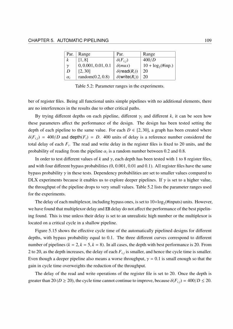
CHAPTER 5. AUTOMATIC PIPELINING 109
Par. Range Par. Rangek [1, 8] δ(Fi, j) 400/Dγ 0, 0.001, 0.01, 0.1 δ(mux) 10 + log2(#inp.)D [2, 30] δ(read(Ri)) 20αi random(0.2, 0.8) δ(write(Ri)) 20
Table 5.2: Parameter ranges in the experiments.
ber of register files. Being all functional units simple pipelines with no additional elements, thereare no interferences in the results due to other critical paths.
By trying different depths on each pipeline, different γi and different k, it can be seen howthese parameters affect the performance of the design. The design has been tested setting thedepth of each pipeline to the same value. For each D ∈ [2, 30], a graph has been created whereδ(Fi, j) = 400/D and depth(Fi) = D. 400 units of delay is a reference number considered thetotal delay of each Fi. The read and write delay in the register files is fixed to 20 units, and theprobability of reading from the pipeline αi is a random number between 0.2 and 0.8.
In order to test different values of k and γ, each depth has been tested with 1 to 8 register files,and with four different bypass probabilities (0, 0.001, 0.01 and 0.1). All register files have the samebypass probability γ in these tests. Dependency probabilities are set to smaller values compared toDLX experiments because it enables us to explore deeper pipelines. If γ is set to a higher value,the throughput of the pipeline drops to very small values. Table 5.2 lists the parameter ranges usedfor the experiments.
The delay of each multiplexor, including bypass ones, is set to 10+log2(#inputs) units. However,we have found that multiplexor delay and EB delay do not affect the performance of the best pipelin-ing found. This is true unless their delay is set to an unrealistic high number or the multiplexor islocated on a critical cycle in a shallow pipeline.
Figure 5.15 shows the effective cycle time of the automatically pipelined designs for differentdepths, with bypass probability equal to 0.1. The three different curves correspond to differentnumber of pipelines (k = 2, k = 5, k = 8). In all cases, the depth with best performance is 20. From2 to 20, as the depth increases, the delay of each Fi, j is smaller, and hence the cycle time is smaller.Even though a deeper pipeline also means a worse throughput, γ = 0.1 is small enough so that thegain in cycle time overweights the reduction of the throughput.
The delay of the read and write operations of the register file is set to 20. Once the depth isgreater than 20 (D ≥ 20), the cycle time cannot continue to improve, because δ(Fi, j) = 400/D ≤ 20.

110 5.4. PIPELINING EXAMPLES
Figure 5.15: Effective cycle time for different pipeline depth for γ = 0.1.
The read operation of the register file becomes the maximum node delay. At this point, deeperpipelines pay a throughput penalty with no cycle time gain.
The bypass probability most sensitive to k increases is γ = 0.1. For smaller bypass probabil-ities, there is a smaller difference between different k’s. As the number of data hazards increases,the number of stalls that each pipeline causes to its neighbors is also larger. If there is a smallamount of stalls, there is a small impact to the throughput. However, if the number of stalls and thenumber of pipelines is large, the number of stalls in the ring increases, producing a more significantdegradation of the throughput due to inter-pipeline communication.
Figure 5.16 shows the effective cycle time for different depths with different bypass probabil-ities (γ is written using letter ’p’ in the figure) and k set to 5. It can be seen that as data hazardfrequency decreases, the number of cycles the pipeline is stalled is smaller, and thus, the perfor-mance of the system is better.
In this example, a better performance is always achieved by assigning each functional unit to itsown pipeline stage, rather than combining them in pairs. Thus, the cycle time for all the differentparameter combinations is δ(Fi, j). It is also interesting to note that the throughput in this example

CHAPTER 5. AUTOMATIC PIPELINING 111
Figure 5.16: Effective cycle time for different pipeline depths for k = 5.
γ D #byp D/#byp cyc ξ cyc ξ
0 20 20 0.850 20 20 40 400.001 20 16.2 0.81 20 35 40 460.01 20 14.2 0.71 20 51 40 710.1 20 6 0.30 20 114 40 136
Table 5.3: Number of bypasses performed in the pipelined design.
is always worse than in DLX examples for similar dependency probabilities. Since there is noshort instruction, like ALU in DLX, all data hazards must stall until the needed instruction finishes.No forwarding is possible.
Table 5.3 shows the number of bypasses per register file done for the best design point explored,for each of the bypass probabilities. As expected, bypass transformations are extensively usedwhen data hazards rarely occur. On the other hand, for bypass probability of 0.1, few bypasstransformations are done and pipelining is achieved by adding bubbles.
The two sets of columns (cyc, ξ) on table 5.3 correspond to 2 of the Pareto points found byRR for the indicated number of bypasses. As γ increases and more bubbles are needed in orderto reach the minimum possible cycle time (20), the effective cycle time distance between using a
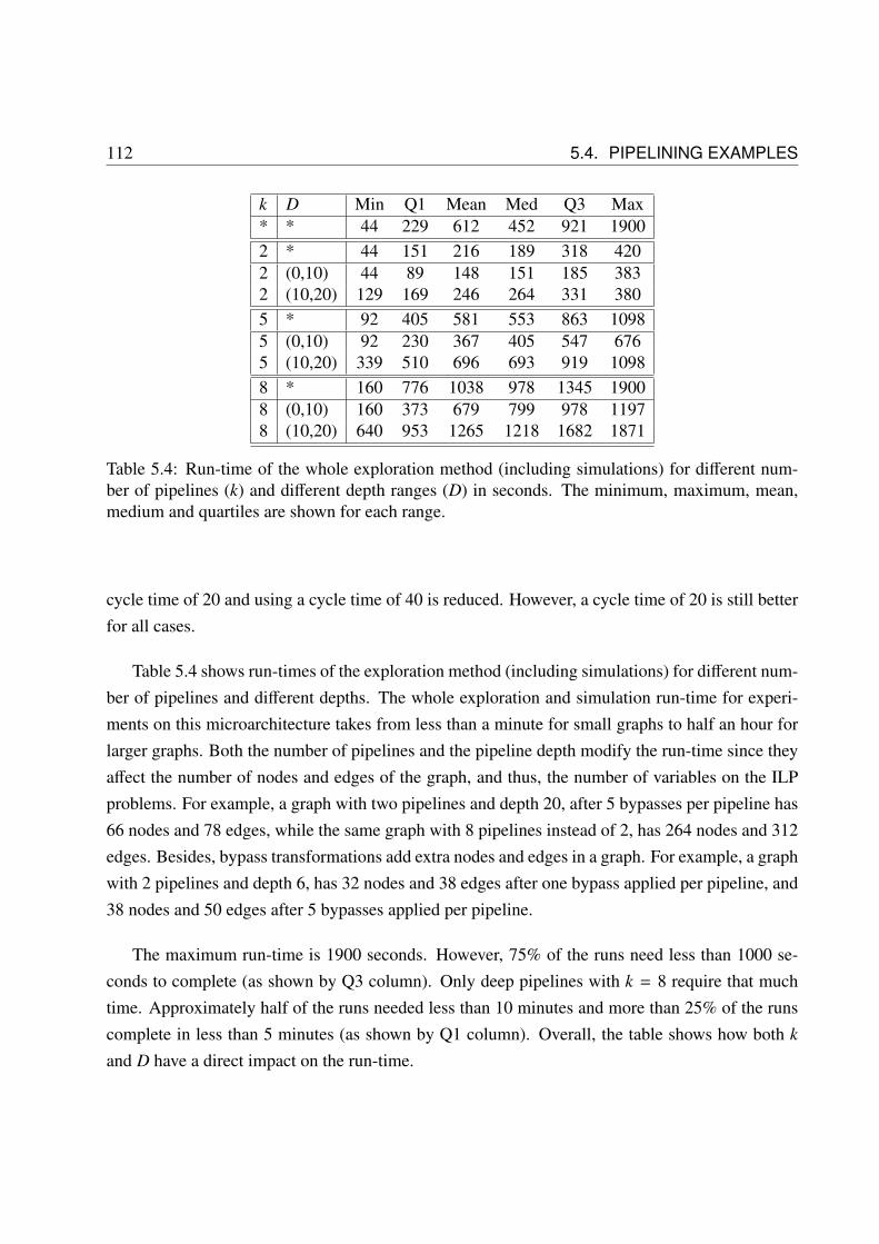
112 5.4. PIPELINING EXAMPLES
k D Min Q1 Mean Med Q3 Max* * 44 229 612 452 921 19002 * 44 151 216 189 318 4202 (0,10) 44 89 148 151 185 3832 (10,20) 129 169 246 264 331 3805 * 92 405 581 553 863 10985 (0,10) 92 230 367 405 547 6765 (10,20) 339 510 696 693 919 10988 * 160 776 1038 978 1345 19008 (0,10) 160 373 679 799 978 11978 (10,20) 640 953 1265 1218 1682 1871
Table 5.4: Run-time of the whole exploration method (including simulations) for different num-ber of pipelines (k) and different depth ranges (D) in seconds. The minimum, maximum, mean,medium and quartiles are shown for each range.
cycle time of 20 and using a cycle time of 40 is reduced. However, a cycle time of 20 is still betterfor all cases.
Table 5.4 shows run-times of the exploration method (including simulations) for different num-ber of pipelines and different depths. The whole exploration and simulation run-time for experi-ments on this microarchitecture takes from less than a minute for small graphs to half an hour forlarger graphs. Both the number of pipelines and the pipeline depth modify the run-time since theyaffect the number of nodes and edges of the graph, and thus, the number of variables on the ILPproblems. For example, a graph with two pipelines and depth 20, after 5 bypasses per pipeline has66 nodes and 78 edges, while the same graph with 8 pipelines instead of 2, has 264 nodes and 312edges. Besides, bypass transformations add extra nodes and edges in a graph. For example, a graphwith 2 pipelines and depth 6, has 32 nodes and 38 edges after one bypass applied per pipeline, and38 nodes and 50 edges after 5 bypasses applied per pipeline.
The maximum run-time is 1900 seconds. However, 75% of the runs need less than 1000 se-conds to complete (as shown by Q3 column). Only deep pipelines with k = 8 require that muchtime. Approximately half of the runs needed less than 10 minutes and more than 25% of the runscomplete in less than 5 minutes (as shown by Q1 column). Overall, the table shows how both k
and D have a direct impact on the run-time.

CHAPTER 5. AUTOMATIC PIPELINING 113
Figure 5.17: Flow for video decoding engine design experiment.
5.5 Video Decoding Engine
A practical test case of optimization using elastic systems is presented in [68]. Among otheroptimization techniques, some of the procedures presented in this chapter were applied in thispaper in order to optimize the critical core of the video decoding engine.
When redesigning an existing synchronous design into a synchronous elastic design (like in thisexperiment), it is natural to separate datapath synthesis and optimization from controller synthesisand optimization, although it must still be possible to connect them afterwards.
The design flow used for the experiment is shown in Fig. 5.17. Starting from the existing RTL,a set of design transformations are applied, such as little care and critical core separation, addingprecomputation, bubble insertion, retiming, etc. These changes are applied manually on the RTL(more details are explained in [68]). To check how these transformations affect timing, area, andpower of the design, we can run a commercial synthesis flow (either logic synthesis only or bothlogic and physical synthesis). These synthesis checks provide feedback to which transformationsshould be accepted and which should be conducted next.
After the desired timing/area/power trade-off is achieved on the datapath, the elastic controlleris generated and merged with the datapath (where registers have been replaced by elastic buffers),producing the new elasticized RTL. This complete new elastic RTL is again synthesized and com-pared to the original design.
The controller generation is automated and follows three steps: RTL2Elastic, MAREX, andSELF compiler. RTL2Elastic is a tool that can analyze an RTL design and produce a microarchitec-tural graph, including early-evaluation multiplexors. The RTL sequential components are grouped

114 5.5. VIDEO DECODING ENGINE
Figure 5.18: Area-performance trade-off of the original and the optimized decoder.
into elastic islands, i.e., several registers are controlled by a single EB controller, as decided bythe user of the tool. Finally, MAREX reads the microarchitectural graph from RTL2Elastic andproduces a Verilog controller of the elastic design using SELF compiler.
MAREX also provides all the elastic transformations and the automatic exploration engine,and it can be used to guide the RTL optimization. After back-annotating the graph with delays ob-tained from synthesis, the tool could automatically suggest elastic transformations, such as retim-ing moves or places where a bubble could be added to enhance the performance. Transformationscould be evaluated quickly before trying them on the RTL.
Furthermore, starting from the original microarchitectural graph, the same transformations thathad been applied on the RTL could be applied on the graph, checking that the results matched.Another decision point was to figure out which of the multiplexors had to be implemented as early-evaluation ones, and which ones should be implemented using simpler controllers. Similarly, fewchannels actually needed to implement token counterflow. Most of them could be implementedusing passive anti-tokens, significantly simplifying the final controller.
Figure 5.18 shows the performance/area trade-off curves between the original synchronousversion of CABAC and the optimized elastic version. These are normalized results after logicsynthesis using a 32 nm library. Given equal area, the cycle time improvement is up to 40%,depending on which cycle time is chosen. Testbench simulations provided a throughput of 0.91 inthe final elastic design. Thus, the effective cycle time speed-up can be up to 35%.

CHAPTER 5. AUTOMATIC PIPELINING 115
5.6 Conclusion
This chapter has presented a method for automatic pipelining of elastic systems. This method takesadvantage of optimization techniques available for elastic systems, such as retiming and recycling,and extends them by exploring different bypass configurations on memory elements of the design.
After applying a number of bypasses to each memory following an heuristic algorithm, andenabling the corresponding forwarding paths to resolve data hazards, the retiming and recyclingoptimization method is called. This method solves a mixed integer linear programming problemwhich models most of the elastic transformations. RR returns a set of non-dominated pipelineconfigurations with different throughput versus cycle time trade-offs. Since the throughput hasbeen estimated inside RR using analysis methods that are not exact, the most promising designpoints are simulated at the end of the exploration in order to obtain their actual throughput.
The presented exploration engine can find hundreds or even thousands of different pipelineswith the same functionality as the original input microarchitecture. The exploration is guided bythe expected instruction frequencies and the expected data dependencies. This way, a pipeline witha near-optimal performance or a good performance/area trade-off for the expected workload can beachieved. The engine can also output a set of Pareto points with different trade-offs between clockcycle, throughput, area and power such that a designer or an architect can select the best suited fora given application.
Using the presented method with different partitions in the functional modules it is possibleto quickly analyze the optimal pipeline depth for a given microarchitecture, conducting pipeliningstudies similar to what is proposed in [72, 79].
The method has been applied to several pipeline designs, showing how different parameters,such as pipeline depth or data hazard probabilities, affect the performance of the system and theshape of the optimal pipeline.
Several extensions can be added to the presented method. Currently, each node is assigned alatency, delay and area. However, it would be possible to assign several possible configurations pernode, each one with a different trade-off between latency (either fixed or variable), combinationaldelay and area. For example, an ALU could have three possible configurations, the first one withthe largest delay, the smallest area and latency of one clock cycle, the second configuration witha smaller delay, larger area and latency of one, and the third configuration with the smallest delaydue to variable latency, but also the largest area. All these possible options could be encoded insidethe RR optimization method, which would be able to pick the best one in function of the criticality

116 5.6. CONCLUSION
of each node.It is also possible to try to apply speculation, as presented in Chapter 4, to some of the configu-
rations found by RR if the throughput is found to be limited by a cycle going through the controlinput of an early-evaluation node, The user should provide a set of pre-defined schedulers thatmust be able to predict some of the choices made inside the system in order to be able to applyspeculation automatically.

Chapter 6
Symbolic Performance Analysis
Elastic systems, either synchronous or asynchronous, can be optimized for the average-case perfor-mance when they have units with early evaluation or variable latency. The performance evaluationof such systems using analytical methods is a complex problem and may become a bottleneckwhen conducting an extensive exploration of different architectural configurations.
This chapter proposes an analytical method for performance evaluation using symbolic expres-sions. The presented method combines timing simulations and symbolic algebraic expressions,and it supports early evaluation and variable-latency units. First, an exact version of this methodwith an exponential worst case complexity is presented. Then, a fast approximate version of thismethod is presented that prunes away low-impact event correlations and computes a lower bound
of the system throughput.
A fast method to estimate the throughput can improve the exploration engine presented inChapter 5. A fast upper bound method already exists in the literature [85, 86], and a fast lowerbound method helps to restrict the actual throughput and to potentially reduce the number of simu-lations needed at the end of the exploration. The contribution presented in this chapter has beenpublished in [63].
6.1 Introduction
Figure 6.1(a) shows a timed marked graph with early evaluation and variable-delay transitions (seeSection 2.1 for an introduction to timed marked graphs). This chapter will introduce Timed multi-
Guarded marked Graphs with Variable-delay (TGVs), an extension to timed marked graphs which
117

118 6.1. INTRODUCTION
t0
t3
t4t5 t6 t7
t1 t21
0.6
0.410 1 1
[(0,0.8),(4,0.2)]1 1
(a) (b) (c)
Figure 6.1: (a) A TGV with early evaluation and variable-delay, (b) AND-causality firing, (c)early-evaluation firing.
can model early-enabling and variable-delay transitions. A formal definition of TGVs is presentedin Section 6.2.1. In Fig. 6.1(a), transitions of the marked graph are represented as thick verticallines, places as the edges between transitions, and tokens as dots over the edges.
Figure 6.1(b) shows conventional AND-causality firing in a marked graph, and Fig. 6.1(c)shows firing with early evaluation, which adds an anti-token into the empty input places of thetransition. In early-evaluation transitions, the selection of the required branch in the datapath isabstracted by using non-deterministic choices. After each firing, the transition chooses which ofthe inputs will be required for the next firing. It can be assumed that it will require only one of theinputs to be valid without loosing generality [85]. Early-evaluation transitions are drawn as specialboxes, like transition t4 in Fig. 6.1(a).
Each input of an early-evaluation transition is assigned a probability that will be used for per-formance analysis. After each firing, early-evaluation transitions choose which input will be re-quired for the next firing using these probabilities. In Fig. 6.1(a), the input from t3 is selected withprobability 0.4, and the input from t0 is selected with probability 0.6.
Each transition is assigned a delay, drawn on top of the transition in Fig. 6.1(a). Transitiont1 has delay 1. This means that once it is enabled, it needs 1 time unit to fire. It is possible fora transition to have several possible delays, modeling variable-latency units. Each possible delayis assigned a probability. For example, transition t3 will need 0 time units to fire with probability0.8 and 4 time units with probability 0.2. It may represent an ALU with a short operation thatcan be computed combinationally and a long operation that needs 4 clock cycles. The delay ofvariable-delay transitions is represented as a set of delay-probability pairs: [(0, 0.8), (4, 0.2)].
The throughput of a TGV is defined as the number of times a transition can fire on averageper time unit. The only work that has studied the performance analysis of systems with early

CHAPTER 6. SYMBOLIC PERFORMANCE ANALYSIS 119
evaluation so far is [85,86]. The paper proposes to use linear programming (LP) in order to obtainan upper bound of the throughput. It does not handle variable-delay transitions directly, but it ismentioned that they can be modeled by using the average delay of the transition (for example 0.8for t3).
This chapter proposes an approach to compute the throughput by extracting the probability dis-tribution of the firing times of transitions. Instead of directly deriving the probability distributionfor each firing time, the presented method derives symbolic expressions, that can correctly captureand manipulate correlations between timing events. Then, the expressions are evaluated to obtainthe firing times of transitions. Finally, the throughput is computed by extracting the average sep-aration between firing times of the same transition. For performance purposes, some correlationsmay be ignored when evaluating the symbolic expressions. It will be shown that a lower bound ofthe throughput is obtained when correlations are ignored.
The throughput of the system in Fig. 6.1(a) is 0.397, obtained by simulating it. However, thelinear programming upper bound method measures 0.449. Consider t2 in Fig. 6.1(a). Since itis enabled at the beginning of the simulation and it has delay 1, its first firing occurs at time 1( f (t2,0) = 1, where f (ti, j) means the time of the j-th firing of transition ti). Similarly, t5 and t7 areinitially enabled ( f (t5,0) = 1, f (t7,0) = 1).
Then, t0, t3 and t6 are enabled. Their firing times are obtained by adding their delays to theirarrival times: f (t0,0) = f (t5,0) + 1 = 2, and f (t6,0) = f (t5,0) + 1 = 2. Since t3 is a variable-delaytransition, the firing time becomes probabilistic. When creating symbolic expressions for firingtimes, variable delays are modeled using variables. As it will be shown, these variables allow todetect correlations due to reconvergent paths. In some cases, these correlations can be simplifiedaway by manipulating the symbolic expression. For this simple example, the firing time of t3 is 0with probability 0.8 and 4 with probability 0.2, and it is captured in variable x0:
x0 = [(0, 0.8), (4, 0.2)]f (t3,0) = f (t2,0) + x0
Transition t4 has an early-evaluation enabling function. When it chooses the lower input, whichhappens with 0.6 probability, its arrival time is the firing time of t0,0. On the other side, when itchooses the upper input, its arrival time is the firing time of t3,0. We can express this firing timeintroducing an early-evaluation operation (∨) in the symbolic expressions:
f (t4,0) = f (t0,0)0.6 ∨ f (t3,0)0.4

120 6.1. INTRODUCTION
When a transition has more than one input and it is not early evaluated, the maximum of thefiring times of the inputs must be computed in order to obtain the arrival time of the transition. Theinputs of t5 are t4 and t7. Hence, the arrival time for f (t5,1) is the maximum of t4,0 and t7,0. Everytime a maximum is created, it is checked whether some of the operands are redundant. In this case,f (t7,0) = 1, and we can derive that f (t4,0) ≥ 1. Thus, f (t7,0) can be discarded:
f (t5,1) = 1 + max( f (t4,0), f (t7,0))= 1 + f (t4,0)
Once the symbolic expressions have been built and simplified, they can be evaluated to obtainthe average firing time, f (t), of each transition. The average firing time of a transition is the meanof the possible delays considering their probabilities.
f (t3,0) = f (t2,0) + x0
= 1 + [(0, 0.8), (4, 0.2)]= [(1, 0.8), (5, 0.2)]
f (t3,0) = 1 · 0.8 + 5 · 0.2 = 1.8
f (t4,0) = f (t0,0)0.6 ∨ f (t3,0)0.4
= 0.6 · 2 + 0.4 · [(1, 0.8), (5, 0.2)]= [(1, 0.32), (2, 0.6), (5, 0.08)]
f (t4,0) = 1 · 0.32 + 2 · 0.6 + 5 · 0.08 = 1.92
f (t5,1) = 1 + f (t4,0)= 1 + [(1, 0.32), (2, 0.6), (5, 0.08)]= [(2, 0.32), (3, 0.6), (6, 0.08)]
f (t5,1) = 2 · 0.32 + 3 · 0.6 + 6 · 0.08 = 1.92
Algorithm 4 shows the top level algorithm to compute the throughput of an elastic system withearly evaluation and variable-latency units. First, an unfolding [61, 107, 119] of the marked graphis created. An unfolding is an acyclic marked graph which “simulates” the behavior of the originalmarked graph for a number of periods. Each transition of the unfolding corresponds to a firingevent of the original marked graph. For example, Fig. 6.2 shows a marked graph which is anunfolding of 2 periods of the marked graph in Fig. 6.1(a), meaning it simulates 2 firings of each

CHAPTER 6. SYMBOLIC PERFORMANCE ANALYSIS 121
Algorithm 4: Overview of the top level algorithm.Input: G : timed marked graph, K : NOutput: The throughput of G
U = CreateEmptyUnfolding()E = CreateEmptyExpressionCollection()done = falseavg f = 0while ¬done do
AddPeriods(G,U,K)for each new transition t ∈ U do
BuildSymbolicExpression(E,U, t)EvaluateExpressions(E)avg fnew = max{AvgFiring(t) | ∀t ∈ G}done = avg f + ε ≥ avg fnew
avg f = max(avg f , avg fnew)return 1/avg f
t2,0 t5,0 t7,0
t6,0t0,0t3,0
t4,0 t1,0
t2,1 t5,1 t7,1
t2,2 t5,2 t7,2
t6,1t0,1t3,1
t4,1 t1,1
Figure 6.2: 2-period unfolding of the marked graph shown in Fig. 6.1(a).
transition.
The algorithm initially builds an unfolding of K periods. The selected K is discussed in Sec-tion 6.4. Then, a symbolic expression is built to represent the firing time of each transition in theunfolding. Each time a maximum or early-evaluation operator is added, some simplification stepsare attempted using max-plus algebra properties in order to optimize the size of the expressions

122 6.1. INTRODUCTION
(and hence the efficiency of the whole method). Finally, the expressions are evaluated to find thefiring time of each transition.
In Section 6.2, it is shown that the throughput can be found by computing the inverse of themaximum, among the transitions of the marked graph, of the average time distance between con-secutive firings in an unfolding which is long enough. After evaluating the expressions, this ma-ximum is computed. While the throughput computed does not converge, more periods are addedto the unfolding incrementally. Section 6.4 shows that convergence always occurs and relates it tothe accuracy of the throughput calculation.
For example, the following table shows the firing times of t2 for 11 periods. Furthermore, thetime distance between firings and the average firing time distance are also shown. The bottom rowsof the table show the average firing time when the initial events are ignored:
Avg( j) = { f (t2,i) − f (t2, j))/(i − j),∀i > j}
Transition t2,0 t2,1 t2,2 t2,3 t2,4 t2,5 t2,6 t2,7 t2,8 t2,9 t2,10
f (t2,i) 1 4 5.92 8.432 10.864 13.3688 15.8787 18.3958 20.9153 23.4369 25.9596
Time dist. − 3 1.92 2.512 2.432 2.5048 2.5099 2.5171 2.5195 2.5216 2.5227
Avg.(0) − 3 2.46 2.4773 2.466 2.4738 2.4798 2.4851 2.4894 2.493 2.496
Avg.(1) − − 1.92 2.216 2.288 2.3422 2.3757 2.3993 2.4165 2.4296 2.44
Avg.(2) − − − 2.512 2.472 2.4829 2.4897 2.4952 2.4992 2.5024 2.505
Avg.(3) − − − − 2.432 2.4684 2.4822 2.491 2.4967 2.5008 2.5039
Avg.(4) − − − − − 2.5048 2.5073 2.5106 2.5128 2.5146 2.5159
Avg.(5) − − − − − − 2.5099 2.5135 2.5155 2.517 2.5182
Avg.(6) − − − − − − − 2.5171 2.5183 2.5194 2.5202
Avg.(7) − − − − − − − − 2.5195 2.5206 2.5213
Avg.(8) − − − − − − − − − 2.5216 2.5221
Avg.(9) − − − − − − − − − − 2.5227
The separation between two consecutive events stabilizes around 2.52, and the average distancebetween events would also converge to 2.52 if more firings where shown. As shown in the table,ignoring the initial firing times makes the average firing time distance converge faster, since onlythe steady state of the marked graph is considered. By definition, the throughput is the inverse ofthe average separation between firings of the same transition. Therefore, 1/2.52 = 0.3968, which

CHAPTER 6. SYMBOLIC PERFORMANCE ANALYSIS 123
is similar to the throughput obtained by simulating during 10000 cycles, 0.3970.The rest of this chapter is structured as follows. First, Section 6.2 defines the problem to be
solved and other important concepts, such as timed marked graphs that can model variable-delaytransitions and early evaluation. This section also relates the throughput to the average time dis-tance between firings of a transition. Then, Section 6.3 defines a max-plus algebra extended withearly evaluation that will be used to model the firing time of each transition. It also shows howto build max-plus algebra expressions from an unfolding and which simplification steps are per-formed to minimize the size of the expressions. Two methods to evaluate the symbolic expressionsare presented: an exact method with exponential time cost, A_exact, and an upper bound methodwith linear time cost, A_prune. The complexity of each method is discussed. Next, Section 6.4discusses the convergence of both algorithms. Finally, Section 6.5 shows some results and Sec-tion 6.6 discusses a possible simplification method for symbolic expressions using SAT-modulotheories (SMT), which was not used due to performance reasons.
6.2 Problem Formulation
This section defines the problem to be solved and some basic concepts needed to understand thesolution. The reader is assumed to be familiar with basic Petri nets concepts. See Section 2.1 forsome basic definitions and read [115] for a tutorial.
The objective of this work is to determine the throughput of an elastic system with early eva-luation and variable-latency units by analyzing a symbolic timing simulation of this elastic system.First, an extension of marked graphs that allow to model the kind of elastic systems under analysis,Timed Multi-Guarded Marked Graph with Variable-Delay, are formally defined. Next, unfoldingsare presented. In this work, unfoldings are used to perform a finite timing simulation of a markedgraph. Finally, the throughput of an elastic system is defined and it is related to the average timedistance between consecutive firings of a transition in a marked graph. Thus, it is shown how thethroughput can be obtained by computing the firing times of an unfolding.
6.2.1 Multi-guarded Marked Graph
Definition 1 (TGV) A Timed Multi-Guarded Marked Graph with Variable-Delay (TGV) is a tuple
N = 〈P,T, Pre, Post,G,m0, δ, α〉 where:
• P is a finite set of places, and T is a finite set of transitions.

124 6.2. PROBLEM FORMULATION
• Pre : P× T → N∪ {0} and Post : P× T → N∪ {0} are the pre and post incidence functionsthat specify the arc weights. The incidence matrix of the net is C = Post − Pre.
• The preset and postset of a node x ∈ P ∪ T are denoted as •x and x•. The Petri net is amarked graph:
∀p ∈ P, |•p| = |p•| = 1.
• m0 : P→ Z assigns an initial number of tokens to each place (the initial marking).
• G : T → 22Passigns a set of guards to every transition. The following conditions must be
satisfied:
a) ∀g ∈ G(t) g ⊆ •t. Each guard is a sub-set of the input places of the transition.b)⋃
g∈G(t) g = •t. Each input place of the transition is at least in one guard.
• α : G → R+ assigns a strictly positive probability to each guard such that for every multi-guarded transition t, ∑
g∈G(t)
α(g) = 1.
• δ : T → {(d, p)} assigns a list of delay-probability pairs to every transition. It must hold thatdi ∈ R
+ ∪ {0} and for every t, ∑(d,p)∈δ(t)
p = 1.
This definition is an extension of the definition of a Timed Multi-Guarded Marked Graph in[85]. The difference is that each transition is assigned a list of possible delays, instead of a singlereal delay. The delay of each transition t, described by a set of pairs delay-probability {(d, p)},represents the number of time units (clock cycles in a latency-insensitive design) that t needs tofire a token. If the delay is equal to 0, it means the transition fires immediately, acting like acombinational circuit. The average delay of a set of delay-probability pairs is the mean of thedistribution.
δ(t) =∑
(d,p) ∈ δ(t)
d · p (6.1)
The guards of transitions model early evaluation. A regular transition has a single guard corres-ponding to its inputs G(t) = {•t}. On the other hand, a multiplexor with two possible input places,p0 and p1, will have the guards G(t) = {{p0}, {p1}}. Without losing expressive power, it is assumed
CHAPTER 6. SYMBOLIC PERFORMANCE ANALYSIS 125
that all early-evaluation transitions have one guard for each input [85]. An early-evaluation transi-tion with input places p0, . . . pn will have n guards, {{p0}, . . . {pn}}. For example, t4 from Fig. 6.1(a)has two guards, one for the edge (t0, t4) and one for the edge (t3, t4). Each guard is assigned aprobability, α(g), used on simulations and performance analysis to decide how often it is selected.
Note that the marking of a place can be negative, modeling anti-token counters. Negativetokens appear when an early-evaluation transition fires and one of the input places does not have apositive token, as shown in Fig. 6.1(c).
Although other marked graph models of elastic designs include backpressure arcs to describebuffer capacities, we choose not to include them for simplicity. This means it is assumed thatbuffers will always have enough capacity. It would be easy to extend TGVs to include such back-pressure arcs.
Definition 2 (Firing semantics) The dynamic behavior of a TGV system is determined by its firing
rules. The execution of a transition t can be described as follows:
• Guard selection. A guard g(t) ∈ G(t) is selected non-deterministically. Once it is selected, itcannot change until t fires.
• Delay selection. A delay d ∈ δ(t) is selected non-deterministically. Once it is selected, itcannot change until t fires.
• Enabling. Transition t becomes enabled if every place p ∈ g(t) is positively marked.
• Firing. Given a marking m, an enabled transition t can fire leading to a new marking m’such that m’ = m + C(P, t), where C(P, t) is the column of C corresponding to t. The firingis performed right after d time units starting from the enabling of the transition.
• Single-server semantics. No multiple-instances of the same transition can fire simultane-ously. A guard selection is produced for each transition firing, and a transition cannot beenabled again while the previous firing has not completed.
The advantage of this model is that it can precisely model variable-latency units. Since thepossible latencies are known, instead of just their average, it is possible to take into account corre-lations between consequent firings of the same transition. For example, if the i-th firing of transi-tion t has a delay of 3 with probability 0.8, then the (i+1)-th firing will not be enabled during these3 time units with probability 0.8. Most properties that apply to the TGMGs defined in [85] also

126 6.2. PROBLEM FORMULATION
t0
t2
t1
t3t4
t5
(a)
t0,0 t1,0 t3,0
t0,2
t4,0
t1,3 t3,3
t2,3
t5,3
t2,0t3,1
t2,1
t1,1
t5,1t4,1
t4,3
t5,0t0,1
t4,2
t3,2
t5,2
t2,2
t1,2
t0,3
(b)
Figure 6.3: (a) example TGV, (b) 4-period unfolding of Fig. 6.3(a), tk,i stands for the i-th instan-tiation of transition tk. The dashed edges enforce single-server semantics for t5 and t0, the rest ofsingle-server semantics edges are not shown for simplicity.
apply to TGVs, since they are two different timing versions of the Multi-Guarded Marked Graphs
defined in [85]. For simplicity, we restrict ourselves to bounded strongly-connected graphs.
6.2.2 Unfoldings
An unfolding of a marked graph [61, 107, 119] is an acyclic marked graph, where each transitioncorresponds to the firing of one of the transitions in the original marked graph. An unfolding canbe divided into periods. The i-th period contains the i-th instantiation of each event.
An unfolding of a Petri net P = {P,T, F,M0} is a tuple U = (B, E, F′, π) where (B, E, F′) isan occurrence net (a subclass of Petri net which is bounded, acyclic, has no auto-conflicts and nobackward branching) and π is a morphism which assigns transitions and arcs of U to transitionsand arcs of P respectively.
Each transition b ∈ B is a tuple b = (t, i), where t ∈ T is the corresponding transition in thePetri net (π(b) = t) and i is a natural number which indicates the firing count of t for the prefixof the unfolding developed up to (t, i). Similarly, the arcs (aka events) in the unfolding reproducethe structure of the original Petri net while being consistent with the instantiation counters of thetransitions.
For example, the marked graph in Fig. 6.3(b) is an unfolding of four periods from the marked

CHAPTER 6. SYMBOLIC PERFORMANCE ANALYSIS 127
graph in Fig. 6.3(a)1. Initially, the transitions t1, t3, t0 from the marked graph are enabled. Thus, inthe unfolding they are the first ones to fire (t1,0, t3,0, t0,0), where tk,i means the i-th firing of transitiontk (π(tk,i) = tk). The firing of t0 enables the second firing of t1 and t3 (t1,1, t3,1), and so on.
6.2.3 Single-Server Semantics
In order to model elastic systems properly, the transitions of a TGV have single-server semantics,i.e., each firing can only start once the previous firing finished. In order to ensure single-server
semantics, some extra edges must be added to the unfolding. These edges make sure that thetransition is not re-entrant, i.e. the (i + 1)-th occurrence of a transition is not enabled before thei-th occurrence has been fired. For each transition t, a single-server semantic place must be addedfrom ti to ti+1, for all i (see single-server semantics for t0 and t5 in Fig. 6.3(b)).
Adding single-server semantics places for all transitions can significantly increase the numberof edges in the unfolding, and hence the run-time of all the algorithms working on this unfolding.Fortunately, it is not necessary to add them for all transitions. In a synchronous elastic system,where all the delays of the TGV are natural numbers, it is sufficient to add single-server semanticsplaces on transitions with delay greater than 1 and for transitions which have a fan-in greater thanone, since they are the only transitions that can introduce backpressure (the first ones because theyhave not finished computing the previous token, and the second ones because some of the inputsare not available yet). Furthermore, single-server semantics edges must also be added between thefirst and second instantiation (between ti,0 and ti,1). Otherwise, transitions t1,0 and t1,1 in Fig. 6.3(b)could have the same firing time if the delay of t0 was 0.
In Fig. 6.3(b), single-server semantics edges are only needed for t5 if none of the other tran-sitions is variable delay. It is easy to show that the rest of single-server semantics places becomeredundant. For example, the single-server semantics edge between t0,0 and t0,1 already ensuressingle-server semantics between between t1,1 and t1,2, and single-server semantics between t1,2 andt1,3 are ensured by the edge between t5,0 and t5,1.
6.2.4 Throughput
Definition 3 (Steady state throughput) The steady state throughput of a transition t, Θ(t), of a
1The dashed edges enforce single-server semantics for transition t5 and t0, see Section 6.2.3 for further details

128 6.2. PROBLEM FORMULATION
TGV is defined as:
Θ(t) = limτ→∞
σ(t, τ)τ
(6.2)
where τ represents time and σ(t, τ) is the firing count of t at time τ, i.e., it indicates how many
times t has fired at time τ.
The firing process is weakly ergodic if the limit in equation 6.2 exists [30]. It can be shown thatthis limit does exist for a TGV and that it is the same for all transitions [85].
6.2.5 Timing Simulation of a TGV
The throughput of an elastic system can be determined by computing the firing time or occurrence
time of each transition in an unfolding which is long enough. In [118], the occurrence time of theevents of an unfolding is computed in order to obtain the cycle time of an asynchronous circuit withonly AND-causality transitions. The firing time of a transition becomes a probability distributionif there is early evaluation or variable-latency in the system.
Definition 4 (Firing time of a transition of an unfolding) The probability distribution for the fir-
ing time of a transition t in an unfolded TGV can be defined as follows:
P( f (t) ≡ X) = P(δ(t) + max{ f (t′) | t′ ∈ •G(t)} ≡ X) (6.3)
where δ(t) is a shorthand for δ(π(t)).
If t belongs to the set of initial events of the unfolding (•t = ∅), then the probability that thefiring time is equal to X it the probability that its delay is X. Otherwise, the probability that f (t) isX is the probability that the chosen delay for t plus the maximum of the firing times of the inputtransitions (considering their probability of being chosen if the transition is early-evaluated) is X.
Theorem 1 (Steady state throughput using firing times) Let G be a TGV, and t be a transition
of G. The steady state throughput of t is:
Θ(t) = limi→∞
i
f (ti)(6.4)
where ti is the i-th instantiation of t in the unfolding of G, and f (ti) is the average of the firing time
for transition ti.

CHAPTER 6. SYMBOLIC PERFORMANCE ANALYSIS 129
ty,i
tz,i
tw,itx,i
......
Figure 6.4: Portion of an unfolding with reconvergent paths.
Proof. By definition 3, the throughput is σ(t, τ)/τ, where the time τ tends to infinity. Since ti
is the i-th instantiation of t in the unfolding of G, t will have fired i times at time f (ti), on average.Therefore, if τ = f (ti), then
σ(t, τ)τ
=i
f (ti)
�
6.3 Max-plus Algebra with Early Evaluation
Instead of directly computing the firing time of each event in the unfolding, a symbolic expressionfor each firing time is created first. The advantage of using symbolic expressions is that they cancapture correlations that are lost otherwise. Consider the portion of an unfolding shown in Fig. 6.4.Assume that the firing time of tx,i is f (tx,i) = [(4, 0.2), (5, 0.8)]. Then, f (ty,i) = f (tx,i) + δ(ty,i) andf (tz,i) = f (tx,i) + δ(tz,i). If both ty,i and tz,i have unit delay, then f (ty,i) = [(5, 0.2), (6, 0.8)] andf (tz,i) = [(5, 0.2), (6, 0.8)]. To compute the arrival time of tw,i, one must compute the maximumof f (ty,i) and f (tz,i). The resulting firing time if each possible combination is taken into account is:
max
(5, 0.2)(6, 0.8)
, (5, 0.2)(6, 0.8)
=
(max(5, 5), 0.04)(max(5, 6), 0.16)(max(6, 5), 0.16)(max(6, 6), 0.64)
=
(5, 0.04)(6, 0.96)
The previous computation gives a too conservative upper bound. Firing times f (ty,i) and f (tz,i)
are correlated, because they both depend on f (tx,i). It is never the case that f (ty,i) , f (tz,i). Thecorrect computation is max( f (ty,i), f (tz,i)) = [(5, 0.2), (6, 0.8)]. Using symbolic expressions, some

130 6.3. MAX-PLUS ALGEBRA WITH EARLY EVALUATION
correlations can be structurally detected and fixed. For example, if δ(tw,i) = 0, f (tw,i) from Fig. 6.4is:
f (tw,i) = 0 + max( f (tx,i) + δ(ty,i), f (tx,i) + δ(tz,i))= f (tx,i) + max(δ(ty,i), δ(tz,i))= [(4, 0.2), (5, 0.8)] + max(1, 1)= [(5, 0.2), (6, 0.8)]
This section defines an extension to max-plus algebra that allows modeling variable delays andearly evaluation. It is shown how the algebra expressions can be build from an unfolding and howto evaluate them. Two algorithms are provided:
• A_exact, defined in Section 6.3.4, computes the exact probability distribution of each firingtime, but it has an exponential worst-case complexity.
• A_prune, defined in Section 6.3.5, is a variation of A_exact which allows to efficientlyobtain a statistical upper bound of each firing time. Since A_prune returns upper bounds ofthe actual firing times f (t), the throughput of the system obtained from this method will bea lower bound of the actual throughput (see equation 6.4).
6.3.1 Definitions
Max-plus algebra [5] has been previously used in the literature in order to find the cycle time ofasynchronous circuits with AND-causality. It has also been extended to Min-Max functions inorder to perform timing analysis of asynchronous circuits with OR-causality and latch-controlledsynchronous circuits with clock schedules [70].
In these papers, AND-causality join structures are translated to max functions and OR-causalityto min functions. In order to adapt max-plus algebra to elastic systems with early evaluation andvariable latency, besides max operation, a new early-evaluation operation is needed. Furthermore,leaf variables are sets of delay-probability pairs instead of positive real numbers. While someproperties of Max-Min functions are probably lost, some basic useful properties are still maintainedin this algebra.

CHAPTER 6. SYMBOLIC PERFORMANCE ANALYSIS 131
Definition 5 (MPEE expression) A max-plus expression with early evaluation (MPEE), e, is a
term in the grammar:
e B δ | x | e1 + e2 | e1 ∧ e2 | eα11 ∨ eα2
2
where δ is a constant, x is a variable, e1 and e2 are MPEE expressions, and αi are early-evaluation
probabilities. Constants are sets of delay-probability pairs, and variables must be assigned to
sets of delay-probability pairs for evaluation. For every early-evaluation operator, the sum of
probabilities must be 1.
Operator +,∧,∨ represent the sum, max and early-evaluation operations for sets of delay-probability. Let us define a grouping operation on sets of pairs by a simple example:
group{(1, 0.1), (2, 0.3), (1, 0.6)} = {(1, 0.7), (2, 0.3)}
Notice that grouping does not change the average delay or any other statistical metric of the set ofdelays. Now the operations on delay-probability pairs can be defined as follows:
Definition 6 (Addition of two sets of delay-probability pairs) Given two sets of delay-probability
pairs, δ1 = {(d1, p1)}, δ2 = {(d2, p2)}, their addition is the set of delay-probability pairs
group{(d1 + d2, p1 × p2) | (d1, p1) ∈ δ1 ∧ (d2, p2) ∈ δ2}
For example:
(2, 0.4)(3, 0.6)
+ (1, 0.8)(2, 0.2)
= group
(3, 0.32)(4, 0.08)(4, 0.48)(5, 0.12)
=
(3, 0.32)(4, 0.56)(5, 0.12)
Definition 7 (Maximum of two sets of delay-probability pairs) Given two sets of delay-probability
pairs, δ1 = {(d1, p1)}, δ2 = {(d2, p2)}, their maximum is the set of delay-probability pairs
group{(max(d1, d2), p1 × p2) | (d1, p1) ∈ δ1 ∧ (d2, p2) ∈ δ2}
For example:
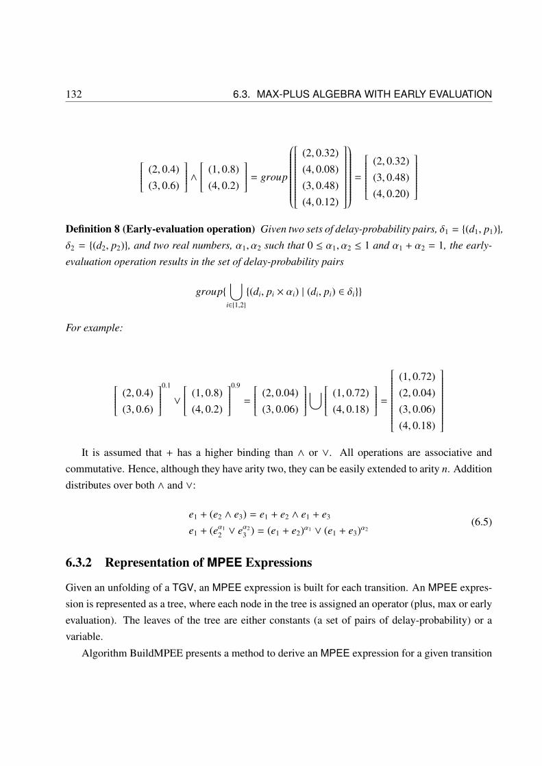
132 6.3. MAX-PLUS ALGEBRA WITH EARLY EVALUATION
(2, 0.4)(3, 0.6)
∧ (1, 0.8)(4, 0.2)
= group
(2, 0.32)(4, 0.08)(3, 0.48)(4, 0.12)
=
(2, 0.32)(3, 0.48)(4, 0.20)
Definition 8 (Early-evaluation operation) Given two sets of delay-probability pairs, δ1 = {(d1, p1)},δ2 = {(d2, p2)}, and two real numbers, α1, α2 such that 0 ≤ α1, α2 ≤ 1 and α1 + α2 = 1, the early-
evaluation operation results in the set of delay-probability pairs
group{⋃
i∈{1,2}
{(di, pi × αi) | (di, pi) ∈ δi}}
For example:
(2, 0.4)(3, 0.6)
0.1 ∨ (1, 0.8)(4, 0.2)
0.9 =
(2, 0.04)(3, 0.06)
⋃ (1, 0.72)(4, 0.18)
=
(1, 0.72)(2, 0.04)(3, 0.06)(4, 0.18)
It is assumed that + has a higher binding than ∧ or ∨. All operations are associative and
commutative. Hence, although they have arity two, they can be easily extended to arity n. Additiondistributes over both ∧ and ∨:
e1 + (e2 ∧ e3) = e1 + e2 ∧ e1 + e3
e1 + (eα12 ∨ eα2
3 ) = (e1 + e2)α1 ∨ (e1 + e3)α2(6.5)
6.3.2 Representation of MPEE Expressions
Given an unfolding of a TGV, an MPEE expression is built for each transition. An MPEE expres-sion is represented as a tree, where each node in the tree is assigned an operator (plus, max or earlyevaluation). The leaves of the tree are either constants (a set of pairs of delay-probability) or avariable.
Algorithm BuildMPEE presents a method to derive an MPEE expression for a given transition
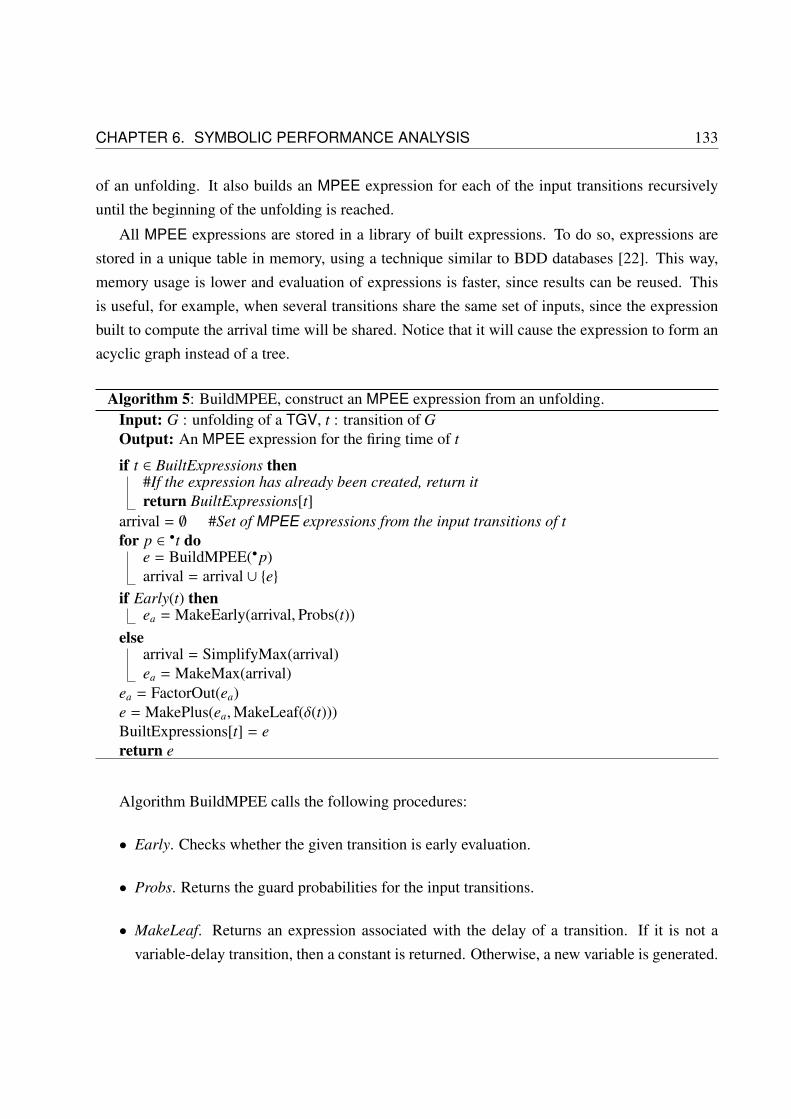
CHAPTER 6. SYMBOLIC PERFORMANCE ANALYSIS 133
of an unfolding. It also builds an MPEE expression for each of the input transitions recursivelyuntil the beginning of the unfolding is reached.
All MPEE expressions are stored in a library of built expressions. To do so, expressions arestored in a unique table in memory, using a technique similar to BDD databases [22]. This way,memory usage is lower and evaluation of expressions is faster, since results can be reused. Thisis useful, for example, when several transitions share the same set of inputs, since the expressionbuilt to compute the arrival time will be shared. Notice that it will cause the expression to form anacyclic graph instead of a tree.
Algorithm 5: BuildMPEE, construct an MPEE expression from an unfolding.Input: G : unfolding of a TGV, t : transition of GOutput: An MPEE expression for the firing time of t
if t ∈ BuiltExpressions then#If the expression has already been created, return itreturn BuiltExpressions[t]
arrival = ∅ #Set of MPEE expressions from the input transitions of tfor p ∈ •t do
e = BuildMPEE(•p)arrival = arrival ∪ {e}
if Early(t) thenea = MakeEarly(arrival,Probs(t))
elsearrival = SimplifyMax(arrival)ea = MakeMax(arrival)
ea = FactorOut(ea)e = MakePlus(ea,MakeLeaf(δ(t)))BuiltExpressions[t] = ereturn e
Algorithm BuildMPEE calls the following procedures:
• Early. Checks whether the given transition is early evaluation.
• Probs. Returns the guard probabilities for the input transitions.
• MakeLeaf. Returns an expression associated with the delay of a transition. If it is not avariable-delay transition, then a constant is returned. Otherwise, a new variable is generated.

134 6.3. MAX-PLUS ALGEBRA WITH EARLY EVALUATION
x2
x1
x0
y2
y1
y0
5,2f(t )
2,2f(t )4,2f(t )
5,1f(t )
1
1 1
1
1
Figure 6.5: Graph representation of an MPEE expression for unfolding in Fig. 6.3(b). xk representsδ(t2,k) and yk represents δ(t4,k).
• MakePlus, MakeMax, MakeEarly. Given a list of input expressions, a new expression iscreated which is either the addition, max or early evaluation of the given list. If the list ofinput expressions has only one element, the same element is returned. MakeEarly receivesa list of probabilities. If an expression with the same operators and operation already existsin memory, then the existing expression is returned. A lower and upper bound for the ex-pression is computed and recorded. Some basic simplifications are done, e.g., constants aregrouped (0 ∧ 1 ∧ e0 = 1 ∧ e0).
• SimplifyMax. Given a list of expressions, it checks whether some of them is subsumed by therest when computing the maximum of the expressions. It uses the upper and lower boundsof the expressions.
• FactorOut. Given an early or max expression, it applies the distributive property in order tofactor out common sub-expressions.
Given the following delays δ(t0) = δ(t5) = 0, δ(t1) = δ(t3) = 1, δ(t2) = δ(t4) = [(1, 0.5), (2, 0.5)];the firing time of t5,2 ( f (t5,2)) in Fig. 6.3(b) is described by the expression graph in Fig. 6.5. In thisfigure, xk is a short-cut for δ(t2,k) and yk is a short-cut for δ(t4,k). It can be seen how expressions arereused to compute different firing times, such as f (t5,2) or f (t5,1).
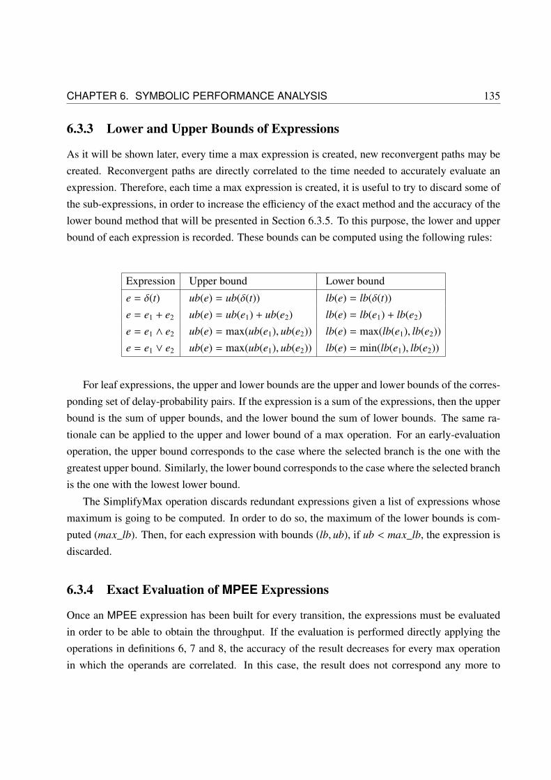
CHAPTER 6. SYMBOLIC PERFORMANCE ANALYSIS 135
6.3.3 Lower and Upper Bounds of Expressions
As it will be shown later, every time a max expression is created, new reconvergent paths may becreated. Reconvergent paths are directly correlated to the time needed to accurately evaluate anexpression. Therefore, each time a max expression is created, it is useful to try to discard some ofthe sub-expressions, in order to increase the efficiency of the exact method and the accuracy of thelower bound method that will be presented in Section 6.3.5. To this purpose, the lower and upperbound of each expression is recorded. These bounds can be computed using the following rules:
Expression Upper bound Lower bound
e = δ(t) ub(e) = ub(δ(t)) lb(e) = lb(δ(t))e = e1 + e2 ub(e) = ub(e1) + ub(e2) lb(e) = lb(e1) + lb(e2)e = e1 ∧ e2 ub(e) = max(ub(e1), ub(e2)) lb(e) = max(lb(e1), lb(e2))e = e1 ∨ e2 ub(e) = max(ub(e1), ub(e2)) lb(e) = min(lb(e1), lb(e2))
For leaf expressions, the upper and lower bounds are the upper and lower bounds of the corres-ponding set of delay-probability pairs. If the expression is a sum of the expressions, then the upperbound is the sum of upper bounds, and the lower bound the sum of lower bounds. The same ra-tionale can be applied to the upper and lower bound of a max operation. For an early-evaluationoperation, the upper bound corresponds to the case where the selected branch is the one with thegreatest upper bound. Similarly, the lower bound corresponds to the case where the selected branchis the one with the lowest lower bound.
The SimplifyMax operation discards redundant expressions given a list of expressions whosemaximum is going to be computed. In order to do so, the maximum of the lower bounds is com-puted (max_lb). Then, for each expression with bounds (lb, ub), if ub < max_lb, the expression isdiscarded.
6.3.4 Exact Evaluation of MPEE Expressions
Once an MPEE expression has been built for every transition, the expressions must be evaluatedin order to be able to obtain the throughput. If the evaluation is performed directly applying theoperations in definitions 6, 7 and 8, the accuracy of the result decreases for every max operationin which the operands are correlated. In this case, the result does not correspond any more to

136 6.3. MAX-PLUS ALGEBRA WITH EARLY EVALUATION
x2
x1
x0
y2
y1
y01
1 1
1
(a)
x0
x1
x2
y0
y1
y21
1 1
1
(b)
Figure 6.6: (a) MPEE expression where x0 and y0 are correlated expressions, the reconvergent pathsfor x0 are dashed, (b) equivalent MPEE expression where x2 and y2 are correlated expressions.
evaluating equation 6.3 correctly.The correlations among different operands of a max expression appear due to reconvergent
paths, as in Fig. 6.4. Both [2] and [101] identify this problem when doing statistical timing analysisof circuits and propose exact solutions with exponential time cost. They identify nodes that are thesources of reconvergent paths, and then they obtain an exact result by evaluating the resulting delayfor each possible combination at the sources of reconvergent paths, merging back all the results toobtain the final result. Given an MPEE expression, it is possible to identify which sub-expressionsare the sources of reconvergent paths by traversing the expression.
Definition 9 (Correlated Expression) Given n MPEE expression e = e1∧e2∧. . . en, an expression
e′ is correlated with respect to e if there are at least two sub-expressions of e, ei, e j, such that there
is a path in the expression graph from ei to e′ and from e j to e′.
Correlated expressions are the sources of a reconvergent path in the expression graph, whichmeans there is a reconvergent path in the unfolding that could not be factored out. The set ofcorrelated expressions for a given max expression can be found by traversing its expression graph.Correlated expressions which evaluate into a single possible delay are not a problem, because itis not necessary to remember there are combinations of delays which are not possible when thereconvergent paths meet again. The set of troublesome correlated expressions are the ones that canincrease the size of a set of delay-probability pairs, which are leaf expressions with more than onepossible delay and early-evaluation expressions.
For example, x0 is a correlated expression in Fig. 6.6(a) with respect to the top max operation ofthe expression graph. The two possible paths to reach x0 from the top of the expression are drawnin dotted lines. The expression graph is symmetric, y0 is also a correlated expression. Symbolic

CHAPTER 6. SYMBOLIC PERFORMANCE ANALYSIS 137
MPEE expressions can alleviate the problem of reconvergent paths since expression manipulationcan factor out common expressions in a max operation. However, there are some cases where thisis not possible. For example, in Fig. 6.6(a), x0 and y0 can be factored out so that they are notcorrelated expressions any more, but then x2 and y2 become correlated expressions, as shown inFig. 6.6(b). There is no way to factor out all of them. The steps performed to reach Fig. 6.6(b)from Fig. 6.6(a) are the following ones:
initial expression (1 + x2 + ((1 + y0) ∧ (x0 + x1)))∧(1 + y2 + ((1 + x0) ∧ (y0 + y1)))
after pushing (1 + x2) and (1 + y2) inside (2 + x2 + y0) ∧ (1 + x2 + x1 + x0)∧(2 + y2 + x0) ∧ (1 + y2 + y1 + y0)
after factoring out (1 + x0) and (1 + y0) (1 + x0 + ((1 + y2) ∧ (x2 + x1)))∧(1 + y0 + ((1 + x2) ∧ (y2 + y1)))
To obtain the exact result of an expression e even if there are correlated expressions, a caseby case evaluation must be performed. For each possible selection of delays in the set corre-lated expressions, e must be evaluated and its result scaled to the selection probability. This way,whenever a max is evaluated, all combinations of delays among the operands are possible and aregular max evaluation can be performed without loosing any accuracy due to correlations. Algo-rithm EvaluateRecursive shows how evaluation case by case can be performed using a recursivealgorithm.
For each correlated expression, it selects all possibilities one by one and calls the algorithmrecursively. The accumulated probability is kept. Once all the correlated expressions have beentraversed, the procedure Eval is called, which evaluates the expression using definitions 6, 7 and8. Eval is a function that will evaluate sub-expressions if it is needed. After evaluation, the partialresult is stored after scaling it with the accumulated probability prob.
For the example in Fig. 6.6(a), the correlated expressions are x0 and y0. If all variables xi andyi have a delay equal to [(1, 0.5), (2, 0.5)], algorithm EvaluateRecursive will branch twice, once forx0 and once for y0. Since each variable has two possible delays, there will be 4 calls to Eval withthe four different combinations of delays:

138 6.3. MAX-PLUS ALGEBRA WITH EARLY EVALUATION
Algorithm 6: EvaluateRecursive, algorithm that evaluates an MPEE expression.Input: e : MPEE expression, i : N, CorrelatedExpr : vector of MPEE expressions, prob : ROutput: Set of delay-probability pairs after evaluating expression e scaled to probabilityprob considering only the i-th first correlated expressions in CorrelatedExpr
if i = 0 thendp = Eval(e) #Evaluate the expression using the selected guards and delaysfor each (d, p) ∈ dp do
#Scale the probability of each delay by multiplying it by probp = p × prob
return dpelse
dp = EmptySetDelayProbability()ce = CorrelatedExpr[i]if Early(ce) then
for each guard (g, p) of ce doSelectGuard(ce, g)dp = group{dp,EvaluateRecursive(e, i − 1,CorrelatedExpr, prob × p)}
else#ce is a leaf expression with variable-delayfor each delay (d, p) of ce do
SelectDelay(ce, d)dp = group{dp,EvaluateRecursive(e, i − 1,CorrelatedExpr, prob × p)}
return dp
Delay combinations Result
x0 = 1, y0 = 1 [(4, 0.0625), (5, 0.5), (6, 0.4375)]x0 = 1, y0 = 2 [(5, 0.125), (6, 0.625), (7, 0.25)]x0 = 2, y0 = 1 [(5, 0.125), (6, 0.625), (7, 0.25)]x0 = 2, y0 = 2 [(5, 0.0625), (6, 0.5), (7, 0.4375)]
Each combination has a probability of 0.25. The final probability distribution is obtained byscaling each distribution by its probability and grouping them together:
[(4, 0.015625), (5, 0.203125), (6, 0.546875), (7, 0.234375)].
The final average firing time is 6.0.Notice that when an expression is evaluated, all its sub-expressions must also be evaluated.

CHAPTER 6. SYMBOLIC PERFORMANCE ANALYSIS 139
These sub-expressions correspond to the input cone of the transition in the unfolding. Thus, it isonly necessary to evaluate the expressions of the newest transitions in the unfolding to obtain allthe firing times.
Algorithm 7: A_exact, algorithm that evaluates an MPEE expression.Input: e : MPEE expressionOutput: Set of delay-probability pairs after evaluating expression e
CorrelatedExpr = FindCorrelatedExpressions(e)numberCorrelatedExpr = size(CorrelatedExpr)#Call the recursive algorithm that will actually evaluate the expressionEvaluateRecursive(e, numberCorrelatedExpr),CorrelatedExpr, 1.0)
Algorithm A_exact evaluates a symbolic expression and all its sub-expressions. It takes intoaccount all correlations, and thus, it computes the exact probability distribution for the firing timeof each transition in the unfolding. It finds the set of correlated expressions structurally by travers-ing the expression, and then it calls EvaluateRecursive. Assuming the length of the unfolding islarge enough, the throughput can be obtained by using equation 6.4.
6.3.5 Upper Bound Evaluation of MPEE Expressions
For most examples, A_exact is infeasible because it is not possible to factor out all correlationsin the MPEE expressions, and the run-time becomes exponential. Algorithm A_prune introducesa couple of heuristics that significantly reduce its complexity. First, the size of the sets of delay-probability pairs must be kept small enough so that operations do not take too much time. Second,some correlated variables and early-evaluation expressions can be ignored and computed as if theydid not add reconvergent paths. A_prune computes an upper bound of the firing times of eachtransition. Therefore, the obtained throughput will be a lower bound of the actual throughput.
Reduction of the Size of Sets of Delay-Probability Pairs
As the expressions grow and have a larger depth, the number of possible delays in the solution alsogrows. Computing max and plus operations has a quadratic cost on the size of the operands. Thus,if δ0 ∧ δ1 is computed, and δ0 is a set of delay-probability pairs with 20 possible delays, and δ1 hasanother 20 possible delays, 400 max operations plus 400 multiplications of probabilities will becomputed.

140 6.3. MAX-PLUS ALGEBRA WITH EARLY EVALUATION
Corner cases tend to have smaller and smaller probabilities. If a variable-delay transition t hasdelay 1 with probability of 0.1, after 10 periods of the unfolding, there will be one delay-probabilitypair with probability 10−10 corresponding to the case where all instantiations of t selected delay 1.
The probability distribution of the firing time of transitions after some periods of the unfoldingtypically has the form of a mountain chain, where the greatest delays and the smallest delays havethe smallest probabilities. One optimization that can reduce the running time with no significantcost on the accuracy of the results is to remove delays with low probability.
After each operation, the set of delays is traversed following increasing order. Neighboring ex-pressions with probabilities lower than a threshold are grouped together into the next delay whichhas a probability higher than the threshold, forming a new pair whose delay is the weighted mean ofthe delays being grouped, to ensure that the total average delay does not change. For example, con-sider the delay [. . . , (9, 0.2), (10, 10−4), (11, 1.5 × 10⁻⁴), (12, 0.1), (13, 0.2), . . .]. If the threshold is10−3, then delay 9 remains unchanged, and delays 10 and 11 are merged into delay delay 12, whichhas a probability larger than 10−3. The resulting delay d and probability p are computed as follows:
p = 10−4 + 1.5 × 10⁻⁴ + 0.1 = 0.10025d = (10 × 10−4 + 11 × 1.5 × 10−4 + 12 × 0.1)/p = 11.9965
Therefore, the new delay is [. . . , (9, 0.2), (11.9965, 0.10025), (13, 0.2), . . .].
A high threshold may force too much grouping, which may actually slow down the computa-tion. Empirically, this value has been set to 10−20. To ensure that results do not grow too much,if the size of the set is larger than some value, for example, 64, some extra grouping may be per-formed with a larger threshold. Notice that this optimization has a negligible impact on the finalaverage firing times, since the probability threshold has been set to a value that is small enough.
Ignoring Correlated Expressions
Some correlations may be completely ignored. In order to do so, the initial call to AlgorithmEvaluateRecursive can be changed so that it does not traverse the whole list of correlated expres-sions, as shown in Algorithm EvaluateUB.
If max_correlated_expr = 2, then only the two first correlated expressions in CorrelatedExprwill be considered. Algorithm A_prune ignores all correlations that have not been simplified duringthe creation of the expressions. It is equivalent to EvaluateUB when max_correlated_expr = 0.Notice that even if max_correlated_expr is 0, some correlations are still taken into account,

CHAPTER 6. SYMBOLIC PERFORMANCE ANALYSIS 141
Algorithm 8: EvaluateUB, algorithm that computes an upper bound of the result of evalua-ting an MPEE expression.
Input: e : MPEE expression, max_correlated_expr : NOutput: Set of delay-probability pairs after evaluating expression e considering onlymax_correlated_expr correlated expressions.
CorrelatedExpr = FindCorrelatedExpressions(e)numberCorrelatedExpr = min(max_correlated_expr, size(CorrelatedExpr))EvaluateRecursive(e, numberCorrelatedExpr),CorrelatedExpr, 1.0)
Algorithm 9: A_prune, algorithm that computes an upper bound of all firing times by ignor-ing all correlations during evaluation.
Input: e : MPEE expressionOutput: Set of delay-probability pairs after evaluating expression e considering nocorrelations during evaluation.
EvaluateRecursive(e, 0, ∅, 1.0)
since they are captured and simplified away when building the MPEE expression in AlgorithmBuildMPEE.
For the example in Fig. 6.5, if only correlations due to x0 are taken into account, only twoevaluations must be done:
Delay combinations Result
x0 = 1 [(4, 0.015625), (5, 0.296875), (6, 0.5625), (7, 0.125)]x0 = 2 [(5, 0.09375), (6, 0.5625), (7, 0.34375)]
Since each combination has a probability of 0.5, the final result is
[(4, 0.0078125), (5, 0.1953125), (6, 0.5625), (7, 0.234375)],
which has an average of 6.02. The exact average firing time was 6. If no correlations are taken intoaccount, then the final result is
[(4, 0.003906), (5, 0.1875), (6, 0.574219), (7, 0.234375)],
which has an average of 6.04. In general, the average firing time increases as the number ofcorrelations considered decreases.

142 6.3. MAX-PLUS ALGEBRA WITH EARLY EVALUATION
Upper Bound Theorem
As the previous example shows, ignoring correlations yields an upper bound of the firing time.Since the throughput of an elastic system is computed using i/ f (ti), the throughput computedignoring correlated expressions will be a lower bound of the real throughput.
Definition 10 (Definition 5 from [2]) A cumulative distribution function (CDF) Q(x) is a statisti-
cal upper bound of another CDF S (x) if and only if for all x, Q(x) ≤ S (x).
Using definition 10, it can be stated that, for each transition ti of the unfolding, the firing timeprobability distribution that A_prune computes for ti is a statistical upper bound of the actual firingtime probability distribution of ti.
Theorem 2 (Theorem 2 in [2]) Let Q,R, S be independent random variables with a lower bound
and an upper bound. Let Q1,Q2 be random variables with CDFs that are identical to the CDF of
Q. The random variable Q1 + R∧Q2 + S is an upper bound of the random variable Q + R∧Q + S .
Let us illustrate this theorem using a simple example. Consider Q = Q1 = Q2 = [(1, 0.3), (3, 0.7)],R = 2, S = 1. Then, Q1 + R = Q + R = [(3, 0.3), (5, 0.7)] and Q2 + S = Q + S = [(2, 0.3), (4, 0.7)].Thus, Q + R ∧ Q + S = Q + R = [(3, 0.3), (5, 0.7)] since we consider only Q. However, since Q1
and Q2 are independent, Q1 + R ∧ Q2 + S = [(3, 0.09), (4, 0.21), (5, 0.7)]. The case in which cor-relations are ignored has one more possible delay (4), and it is a statistical upper bound of the casein which correlations are considered.
This theorem can be extended to handle early-evaluation MPEE expressions using the follow-ing lemmas.
Lemma 3 Let Q be a random variable with a lower bound and an upper bound. Let Q1,Q2 be
independent random variables with CDFs that are identical to the CDF of Q. The CDF of the
random variable Qα11 ∨ Qα2
2 is equal to the CDF of the random variable Qα1 ∨ Qα2 .
Proof. Using the definition of the early-evaluation operation on sets of delay-probability pairs,Qα1 ∨ Qα2 = {(d, p × α1) | (d, p) ∈ Q}
⋃{(d, p × α2) | (d, p) ∈ Q}, and
Qα11 ∨ Qα2
2 = {(d, p × α1) | (d, p) ∈ Q1}⋃{(d, p × α2) | (d, p) ∈ Q2}. Since the pairs of Q1 and the
pairs of Q2 are not combined in any way, a bijection can be built between delay-probability pairsfrom Qα1 ∨ Qα2 and delay-probability pairs from Qα1
1 ∨ Qα22 . Therefore, they have the same CDF.
�

CHAPTER 6. SYMBOLIC PERFORMANCE ANALYSIS 143
Lemma 4 Let R, S be independent random variables with a lower bound and an upper bound. Let
Q be the random variable obtained by Rα1 ∨ S α2 . Let R1,R2 be independent random variables with
the same CDF as R and S 1, S 2 be independent random variables with the same CDF as S . Finally,
let Q1,Q2 be independent random variables built by the expression Qi = Rα1i ∨ S α2
i , i ∈ {1, 2}. The
random variable Q1 ∧ Q2 is an upper bound of the random variable Q ∧ Q.
Proof. It must be shown that for every possible x, P(Q1 ∧ Q2 ≤ x) ≤ P(Q ∧ Q ≤ x).
Using the maximum and early evaluation definition:
P(Q ∧ Q ≤ x) = α1 × P(R ∧ R ≤ x) + α2 × P(S ∧ S ≤ x),P(Q1 ∧ Q2 ≤ x) = α2
1 × P(R1 ∧ R2 ≤ x)+ α1 × α2 × P(R1 ∧ S 2 ≤ x)+ α2 × α1 × P(S 1 ∧ R2 ≤ x)+ α2
2 × P(S 1 ∧ S 2 ≤ x).
In the second case, Q1 can choose one guard and Q2 can choose the other guard since there isno correlation between them. Next, it will be shown that
α1 × P(R ∧ R ≤ x) ≥ α21 × P(R1 ∧ R2 ≤ x) + α1 × α2 × P(R1 ∧ S 2 ≤ x).
The same can be shown for the second halves of the previous expressions.
Using the definition of the maximum operation (definition 7),
α1 × P(R ∧ R ≤ x) = α1 ×∑{p | (d, p) ∈ R ∧ d ≤ x},
α21 × P(R1 ∧ R2 ≤ x) = α2
1 ×∑{p1 × p2 | (d1, p1) ∈ R1 ∧ (d2, p2) ∈ R2 ∧max(d1, d2) ≤ x}
α1 × α2 × P(R1 ∧ S 2 ≤ x) = α1 × α2 ×∑{p1 × p2 | (d1, p1) ∈ R1 ∧ (d2, p2) ∈ S 2 ∧max(d1, d2) ≤ x}.
Each expression can be partitioned depending on which d of the first operand (R or R1) itbelongs to. For the first one, for each pair (d, p) ∈ R such that d ≤ x, its contribution to the total sumis α1 × p. For the second one, its contribution is α2
1 × p ×∑{p2 | (d2, p2) ∈ R2 ∧max(d, d2) ≤ x}
and for the third one it is α1 × α2 × p ×∑{p2 | (d2, p2) ∈ S 2 ∧max(d, d2) ≤ x}.

144 6.3. MAX-PLUS ALGEBRA WITH EARLY EVALUATION
Then, α1 × p can be removed because it is present in all expressions:
α1 × p ≥ α21 × p ×
∑{p2 | (d2, p2) ∈ R2 ∧max(d, d2) ≤ x}
+ α1 × α2 × p ×∑{p2 | (d2, p2) ∈ S 2 ∧max(d, d2) ≤ x}
implies1 ≥ α1
∑{p2 | (d2, p2) ∈ R2 ∧max(d, d2) ≤ x}
+ α2∑{p2 | (d2, p2) ∈ S 2 ∧max(d, d2) ≤ x}
Since∑{p2 | (d2, p2) ∈ R2 ∧max(d, d2) ≤ x} ≤ 1 and
∑{p2 | (d2, p2) ∈ S 2 ∧max(d, d2) ≤ x} ≤ 1
by definition (the sum of probabilities of a set of delay-probability pairs is 1), and α1 + α2 = 1, theprevious inequality holds. �
Finally, the theorem that states that MPEE expression evaluation ignoring some correlationsprovides an statistical upper bound of the evaluation considering all correlations can be stated andproved.
Theorem 5 Let e be an MPEE expression representing the firing time of transition ti of the unfold-
ing. Let Q(x) be the CDF of the probability distribution computed by using definitions 6, 7 and 8
on e, and let S (x) be the probability distribution which is the solution of equation 6.3 for transition
ti. Q(x) is a statistical upper bound of S (x).
Proof. The proof can be partitioned into different parts depending on the structure of e. S (x)corresponds to evaluating e using the exact method which has already been presented.
If e is a leaf, then the solution is the probability distribution given by the δ(t). Therefore,Q(x) = S (x). Lemma 3 shows that theorem 5 holds when e is an early-evaluation operation,theorem 2 and lemma 4 show that theorem 5 holds when e is a maximum. This theorem does nothold for addition, i.e., Q1(x) + Q2(x) is not an statistical upper bound of Q(x) + Q(x), where Q,Q1
and Q2 are identical probability distributions. For example, if Q = Q1 = Q2 = [(0, 0.5), (1, 0.5)],Q + Q = [(0, 0.5), (2, 0.5)] and Q1 + Q2 = [(0, 0.25), (1, 0.5), (2, 0.25)]. The mean in both cases is1, but [(0, 0.25), (1, 0.5), (2, 0.25)] is not an statistical upper bound of [(0, 0.5), (2, 0.5)]. However,by construction of MPEE expressions in unfoldings, the same expression is never added to itself,it is always added to the delay of another transition. If the same expression was added to itself, itwould mean that an event is being counted twice. Therefore, this case can be ignored. �
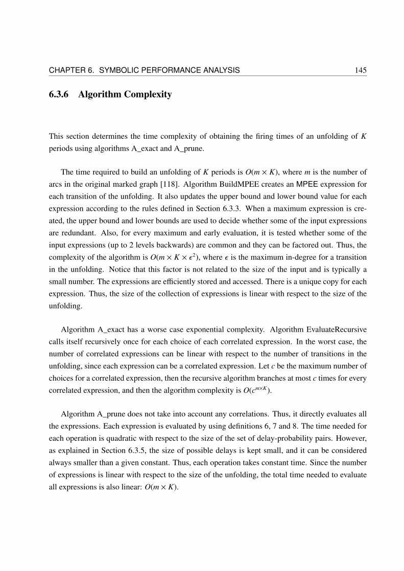
CHAPTER 6. SYMBOLIC PERFORMANCE ANALYSIS 145
6.3.6 Algorithm Complexity
This section determines the time complexity of obtaining the firing times of an unfolding of K
periods using algorithms A_exact and A_prune.
The time required to build an unfolding of K periods is O(m × K), where m is the number ofarcs in the original marked graph [118]. Algorithm BuildMPEE creates an MPEE expression foreach transition of the unfolding. It also updates the upper bound and lower bound value for eachexpression according to the rules defined in Section 6.3.3. When a maximum expression is cre-ated, the upper bound and lower bounds are used to decide whether some of the input expressionsare redundant. Also, for every maximum and early evaluation, it is tested whether some of theinput expressions (up to 2 levels backwards) are common and they can be factored out. Thus, thecomplexity of the algorithm is O(m × K × ε2), where ε is the maximum in-degree for a transitionin the unfolding. Notice that this factor is not related to the size of the input and is typically asmall number. The expressions are efficiently stored and accessed. There is a unique copy for eachexpression. Thus, the size of the collection of expressions is linear with respect to the size of theunfolding.
Algorithm A_exact has a worse case exponential complexity. Algorithm EvaluateRecursivecalls itself recursively once for each choice of each correlated expression. In the worst case, thenumber of correlated expressions can be linear with respect to the number of transitions in theunfolding, since each expression can be a correlated expression. Let c be the maximum number ofchoices for a correlated expression, then the recursive algorithm branches at most c times for everycorrelated expression, and then the algorithm complexity is O(cm×K).
Algorithm A_prune does not take into account any correlations. Thus, it directly evaluates allthe expressions. Each expression is evaluated by using definitions 6, 7 and 8. The time needed foreach operation is quadratic with respect to the size of the set of delay-probability pairs. However,as explained in Section 6.3.5, the size of possible delays is kept small, and it can be consideredalways smaller than a given constant. Thus, each operation takes constant time. Since the numberof expressions is linear with respect to the size of the unfolding, the total time needed to evaluateall expressions is also linear: O(m × K).

146 6.4. NUMBER OF PERIODS OF THE UNFOLDING
6.4 Number of Periods of the Unfolding
The final question that needs to be answered is how many times the TGV should be unfolded, forboth A_exact and A_prune algorithms. In [118], an upper bound of the periods of an unfolding isfound, so that it can be guaranteed that the exact cycle time is correctly computed. Unfortunately,variable latency and early evaluation make this result invalid, although some other results from thepaper still hold. A dynamic algorithm is used to determine the number of periods for the unfolding.This section presents some theoretical background to justify this dynamic algorithm.
6.4.1 Convergence of A_exact
In order to remove the effect of variations in the initial stages of the timing simulation, beforethe steady state has been reached, the notion of event-initiated timing simulation is introduced.When performing an event-initiated timing simulation, the firing times of the transitions that arenot reachable from the initiator are assigned a firing time of 0.
Definition 11 (Event-initiated timing simulation) A timing simulation is initiated by event e if
all the events that are not reachable from e in the unfolding are assumed to have a firing time of 0,
i.e., fe(g) = 0 iff (e = g or e; g), where (e ⇒ g) means that there is a path in the unfolding from
e to g.
The following proposition helps to prove that the average separation between occurrences ofthe same transition (and hence the throughput) can be computed using the maximum operation.
Proposition 3 from [118] (Triangular Inequality). For a ti-initiated timing simulation, the oc-
currence time of a later instantiation of transition t ( f ti(tk)), k > i, is larger than or equal to the
sum of any combination of occurrence times for instantiations with occurrence indices between i
and k and a total occurrence period equal to k − i:
∀t,∀i ≥ 0,∀k > i : f ti(tk) ≥ max{ f ti(t j) + f ti(t(i+k− j)) | i < j < k}
This proposition holds also for systems with early evaluation and variable-delay transitions. Inan unfolding with a finite number of periods, there is a finite number of delay and guard choices.Assume that for each possible choice (that is, for each combination of delays in the variable-delaystransitions and guard selections in early-evaluation units), a separate identical unfolding is created.

CHAPTER 6. SYMBOLIC PERFORMANCE ANALYSIS 147
In each copy, for each early evaluation transition, the places whose guards have not been selectedare removed, and each variable-latency transition has chosen only one delay. In the unfolding ofFig. 6.3(b), if t2 and t4 have delay [(1, 0.5), (2, 0.5)], the rest of the transitions have a single latencyand there is no early evaluation, there are 4 transitions with delay choices: t2,0, t2,1, t4,0, and t4,1;and each one can choose between two delays, 1 or 2. Thus, there are 24 possible combinations.Since each delay has probability 0.5, the probability of each combination is 0.54. The number ofcombinations grows as the number of periods in the unfolding grows. Each copy of the unfoldingis a simple elastic system, with neither early evaluation nor variable latency. Hence, proposition 3holds for each of these unfoldings as proven in [118].
The probabilistic firing time of each transition for the original unfolding can be obtained byadding the firing time of each combination multiplied by the combination probability. In the previ-ous example, it would be necessary to add the firing time of each of the 24 combinations multipliedby 0.54. Since each of the unfoldings without early evaluation and variable latency honors propo-sition 3, and the set of all these unfoldings correspond to all the possible behaviors of the originalunfolding, proposition 3 also holds for the probabilistic case. It can be inferred by induction thatproposition 3 also holds on an infinite unfolding.
Definition 12 (Separation between occurrences) The separation between two occurrences of the
same transition t, ti and t j, is defined as:
∆i(t j) =f ti(t j)j − i
(6.6)
Using the triangular proposition, the throughput can be related to the separation between oc-currences for any transition t:
maxi, j{∆i(t j)} ≤ 1/Θ (6.7)
That is, the estimation of the throughput computed as an inverse of the average separation betweenoccurrences over some length of simulation is an upper bound on the exact throughput.
The limit from the throughput definition (equation 6.4) exists, as pointed out in Section 6.2.4.Equation 6.7 is monotonically improving the bound because of the maximum operation. Thelonger the unfolding, the closer equation 6.7 gets to the exact throughput. Furthermore, we canderive from the triangular inequality that f ti(tk) ≥ f ti(t j) + f ti(ti+k− j), which points that the separa-tion between occurrences will keep increasing until max{∆i(t j)} = 1/Θ. Therefore, we can assure

148 6.4. NUMBER OF PERIODS OF THE UNFOLDING
that we can reach any level of accuracy to the throughput estimation by creating a long enoughunfolding:
∀ε > 0, ∃ k > 0, max∀k≥ j>i≥i0
{∆i(t j)} ≥ (1 − ε) · 1/Θ (6.8)
where ε is a small number that can be tuned to decide the acceptable error of the algorithm, and i0
is a constant that avoids taking into account initial perturbations (empirically set to a tenth of thelength of the unfolding). This equation justifies the following algorithm. Iteratively, a number ofperiods is added to the unfolding. Then, the firing times for the new transitions are computed. LetA_exact(k) be max∀k≥ j>i≥i0{∆i(t j)}, the result obtained by running A_exact algorithm on a k-periodunfolding. First, A_exact(T/2) is computed, where T is the number of tokens in the TGV. Next,T/2 periods are added at each iteration, until the result stabilizes:
A_exact(i · T/2) + (1 − ε) ≥ A_exact((i + 1) · T/2),Any constant N can be used in place of T/2, but T/2 scales together with the size and the
complexity of the TGV, and it works well based on experiments. Experimentally, convergence istypically reached with less than 3T periods in the unfolding.
Instead of performing an event-initiated timing simulation for every transition in the markedgraph, it is enough to do so for a cut-set of the transitions. A cut-set of a marked graph is a setof transitions such that each cycle in the graph contains at least one of the transitions. Ideally, aminimum cut-set would optimize the total run-time, but finding this minimum cut-set is a difficultproblem by itself. However, the set of transitions such that they have some token at the inputs is afast way to obtain a cut-set, since all cycles have at least one token.
6.4.2 Convergence of the Upper Bound Method, A_prune
The dynamic method to decide when to stop adding periods to the unfolding can also be appliedto A_prune algorithm. For every transition in the unfolding ti, A_prune computes a firing timeprobability distribution f ub(ti) which is a statistical upper bound of f (ti). There are two importantfacts to consider::
1. By construction, the upper bound of both distributions is the same, ub( f ub(ti)) = ub( f (ti)).
2. Since each max expression which has correlated expressions adds some extra overhead tothe upper bound, and no other type of operation modifies the accuracy of the result,
f ub(ti) = f (ti) + k =⇒ f ub(ti+1) ≥ f (ti+1) + k

CHAPTER 6. SYMBOLIC PERFORMANCE ANALYSIS 149
Due to the second item, the estimation of the average occurrence distance based on the up-per bound, f ub(ti), cannot decrease with iterations, and due to the first item, it is always limitedfrom above. Hence the difference between the actual firing time and its computed upper bound isbounded, and it cannot decrease if more periods are added to the unfolding.
Let Θlb be the throughput returned by applying A_prune to an infinite unfolding. Consideringthat f ub(ti) ≥ f (ti), it can be derived that Θlb ≤ Θ. If the previously defined dynamic methodis applied to A_prune, it will return a throughput Θlb/ε, where ε ≤ 1. It must be ensured thatΘlb/ε ≤ Θ, because the objective of this method is to obtain a lower bound of the throughput.Since A_prune is a fast algorithm, the accuracy parameter ε in the dynamic algorithm can be setto a small enough value so that the resulting throughput will either be a lower bound of the Θ or itwill be equal to Θ for enough significant digits.
6.4.3 Example
Figure 6.7(b) shows the throughput of the TGV in Fig. 6.7(a) with different number of periods inthe unfolding and different correlation strategies. In Fig. 6.7(a), the number below each transitionrepresents its delay. There is one early-evaluation transition and one variable-delay transition. Thethroughput obtained by simulating the elastic system is 0.537. The throughput obtained by thelinear programming method in [85] is 0.618.
The two horizontal lines in Fig. 6.7(b) correspond to the simulation throughput and the LPthroughput. A_prune(k) is defined similarly to A_exact(k), the result obtained by running A_prunealgorithm on a k-period unfolding. The other three lines correspond to A_exact(k), A_prune(k),and a third algorithm where max_correlated_expr (presented in Section 6.3.5) has been set to 12.The reader should keep in mind that the figure shows the throughputs, which are the inverse of theaverage firing times.
It can be seen that A_exact(k) complies with equation 6.7. The computed throughput is al-ways greater than the simulation throughput, and after 5 periods it converges, returning the exactthroughput.
A_prune is initially over the throughput, but after 3 periods it crosses the line representing thesimulation throughput. As it has been explained, it is possible that this happens if the unfolding istoo short. However, it converges at 0.470, which is indeed a lower bound of the throughput.
The plot for max_correlated_expr = 12 behaves exactly like A_exact while there are lessthan 12 correlated expressions, since it can capture all correlations and compute all firing times
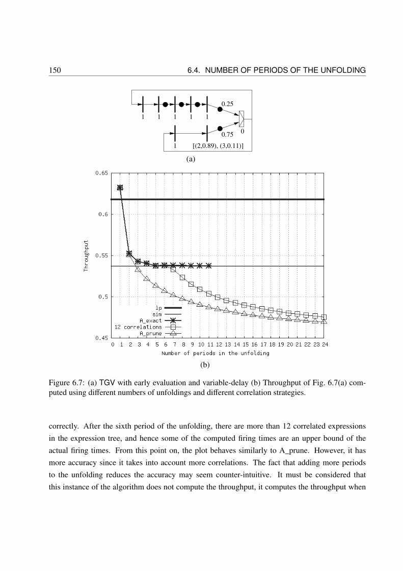
150 6.4. NUMBER OF PERIODS OF THE UNFOLDING
1 1 1 1 1
1
0
[(2,0.89), (3,0.11)]
0.25
0.75
(a)
(b)
Figure 6.7: (a) TGV with early evaluation and variable-delay (b) Throughput of Fig. 6.7(a) com-puted using different numbers of unfoldings and different correlation strategies.
correctly. After the sixth period of the unfolding, there are more than 12 correlated expressionsin the expression tree, and hence some of the computed firing times are an upper bound of theactual firing times. From this point on, the plot behaves similarly to A_prune. However, it hasmore accuracy since it takes into account more correlations. The fact that adding more periodsto the unfolding reduces the accuracy may seem counter-intuitive. It must be considered thatthis instance of the algorithm does not compute the throughput, it computes the throughput when

CHAPTER 6. SYMBOLIC PERFORMANCE ANALYSIS 151
Table 6.1: Experimental results on random graphs with early-evaluation nodes and no variable-latency units. N: nodes, E: edges, EV: early-evaluation nodes, VD: variable-delay nodes, T: tokens,EBs: number of EBs, UB: upper bound throughput (LP), SIM: simulation throughput, LB: lowerbound throughput, ∆UB: UB error w.r.t. SIM, ∆LB: LB error w.r.t. SIM.
Graph Throughput ErrorGraph N E EV VD T EBs UB SIM LB ∆UB ∆LB
G0 9 10 1 0 2 4 0.500 0.500 0.500 0% 0%G1 9 10 1 0 2 4 0.412 0.412 0.412 0% 0%G2 9 10 1 0 5 8 0.765 0.732 0.656 5% -10%G3 18 28 4 0 10 28 0.619 0.472 0.429 31% -9%G4 48 66 6 0 15 39 0.254 0.253 0.253 0% 0%G5 56 77 6 0 21 46 0.250 0.239 0.235 5% -2%G6 54 74 8 0 38 60 0.713 0.702 0.696 2% -1%G7 70 94 12 0 33 45 0.867 0.805 0.801 8% 0%G8 59 142 11 0 53 129 0.250 0.217 0.199 15% -8%G9 180 619 47 0 139 340 0.333 0.321 0.305 4% -5%
only 12 reconvergent paths can be considered, which happens to be a lower bound of the actualthroughput. This lower bound is found when the plot converges, at 0.475.
6.5 Experimental Results
This section presents a set of experiments with random graphs. Each graph has been producedin three different flavors, only with early evaluation, only with variable-latency units, and withboth early evaluation and variable-latency, to show the accuracy of the presented method in eva-luating both features. The applicability of both the lower bound and the upper bound method forperformance analysis during a design space exploration is shown on a set of experiments.
6.5.1 Random Graphs
To show the accuracy of the presented method, a set of experiments has been performed on se-quential circuits from the MCNC benchmarks. For each circuit, the graph structure was extracted,and the largest strongly connected component was saved. Then, each edge was assigned a tokenwith a random probability between 0.25 and 0.6. Next, each transition was assigned unit delaywith a random probability greater than 0.5, otherwise its delay was set to zero. Variable delayswere added to 10% of the nodes. These nodes were assigned two random possible delays between

152 6.5. EXPERIMENTAL RESULTS
Table 6.2: Experimental results on random graphs with variable-latency units and no early-evaluation nodes. Legend is the same as in Table 6.1.
Graph Throughput ErrorGraph N E EV VD T EBs UB SIM LB ∆UB ∆LB
G0 9 10 0 1 2 4 0.287 0.287 0.264 0% -8%G1 9 10 0 2 2 4 0.107 0.107 0.101 0% -6%G2 9 10 0 1 5 8 0.322 0.322 0.308 0% -4%G3 18 28 0 2 10 28 0.333 0.199 0.172 67% -14%G4 48 66 0 5 15 39 0.161 0.133 0.126 21% -5%G5 56 77 0 3 21 46 0.182 0.175 0.172 4% -2%G6 54 74 0 7 38 60 0.476 0.265 0.251 80% -5%G7 70 94 0 5 33 45 0.526 0.272 0.229 93% -16%G8 59 142 0 3 53 129 0.143 0.143 0.143 0% 0%G9 180 619 0 7 139 340 0.152 0.148 0.127 3% -14%
0 and 10. Each delay was assigned a random probability. Finally, 25% of the nodes with 2 or moreinputs were configured as early-evaluated. The probability of each input was generated randomly.
Tables 6.1, 6.2 and 6.3 show the list of graphs and their throughputs. For each graph, threeversions were created. One with only early-evaluation nodes (shown in Table 6.1), one with onlyvariable-delay nodes (shown in Table 6.2), and one with early evaluation and variable-delay (shownin Table 6.3). Results are compared against the upper bound method (LP) in [85] that uses linearprogramming.
The maximum number of correlations taken into account by the evaluation algorithm was setto 0 in order to obtain the fastest possible run-times. When building the expressions, some correla-tions can already be factored out. For the case where there is only early evaluation and no variable-delay, the average errors for the upper bound method and the lower bound method are 6.8% and3.5% respectively. Both methods are quite accurate, although there are two graphs where the errorof the upper bound method is over 10%.
The LP method is less accurate on graphs with variable-delay nodes since it does not knowthe possible delays of these transitions, it only considers the average delay of the transition. Theaverage errors are 26% and 7% respectively. If both early evaluation and variable-delay nodes aretaken into account, the average errors are 63% and 9%.
The LP solver used to compute the upper bound method is CPLEX. The presented method hasbeen implemented in C++. The experiments have been run on a Xeon processor at 2.66 GHz with3 MB of cache. We have found that a simulation of 10000 cycles typically provides an acceptable

CHAPTER 6. SYMBOLIC PERFORMANCE ANALYSIS 153
Table 6.3: Experimental results on random graphs with early-evaluation nodes and variable-latencyunits. Legend is the same as in Table 6.1.
Graph Throughput ErrorGraph N E EV VD T EBs UB SIM LB ∆UB ∆LB
G0 9 10 1 1 2 4 0.372 0.329 0.288 13% -12%G1 9 10 1 2 2 4 0.207 0.107 0.101 93% -6%G2 9 10 1 1 5 8 0.618 0.538 0.470 15% -13%G3 18 28 4 2 10 28 0.474 0.226 0.180 110% -20%G4 48 66 6 5 15 39 0.169 0.135 0.126 25% -7%G5 56 77 6 3 21 46 0.222 0.181 0.176 23% -3%G6 54 74 8 7 38 60 0.692 0.268 0.257 158% -4%G7 70 94 12 5 33 45 0.656 0.269 0.236 144% -12%G8 59 142 11 3 53 129 0.250 0.199 0.190 26% -5%G9 180 619 47 7 139 340 0.233 0.181 0.164 29% -9%
accuracy, even in graphs which have several variable-latency units with 3 or 4 possible delays and asignificant amount of early-evaluation nodes. If there are fewer delay choices in the elastic system,5000 or even 1000 cycles may be enough simulation time. Figure 6.8 shows the run-times foreach of the evaluated methods in the graphs from Table 6.3. The lower bound method is aroundhalf to one order of magnitude slower than the LP method. Simulations were around 2 orders ofmagnitude slower than the lower bound method. The lower bound run for the biggest graph tookaround 8 seconds. The rest of the runs took less than one second.
6.5.2 Evaluating Relative Performance
If a designer wants to compare several possible designs or perform some architectural exploration,it is important that the order between designs on simulation and on analysis is the same. A set ofexperiments have been performed in order to determine whether the presented analytical techniquecan correctly order a set of pipelines. If the throughput of pipeline A is higher that the throughputof pipeline B according to the analytical estimation, then it should also be higher in simulation.
Retiming and recycling [24] has been executed on each graph to extract the set of non-dominatedconfigurations. Each of these configurations is latency equivalent to the original one, and it hasbeen obtained by applying a sequence of elastic transformations, mainly retiming moves and bub-ble insertion. Then, the throughput of each configuration has been obtained by using the linearprogramming upper bound method, the presented lower bound method, and simulation. Finally,the configurations have been ordered using each of the throughputs.

154 6.5. EXPERIMENTAL RESULTS
Figure 6.8: Run-time of the different performance evaluation versions in seconds for the graphsin Table 6.3. LB is the presented lower bound method, UB the linear programming upper boundmethod, and SIM is the simulation time. The Y-axis is in logscale.
Table 6.4 shows the three throughputs (simulation, lower bound and upper bound) for each oneof the 16 configurations found by RR for graph G8. The index of each configuration when orderedby the throughput of the corresponding column is written next to each throughput. The referenceorder is determined by the simulation throughput. In order to achieve the simulation order fromthe upper bound order, one must do 2 swaps: the 6th and 5th configurations must be swapped,and the 13th and 14th configurations must be swapped. The average throughput difference foreach swap is 2.15% (0.8% for the first swap and 3.4% for the second swap). Similarly, 4 swapsare needed to correctly order the order produced by the lower bound analysis, and the averagethroughput difference per swap is 0.76%. These two metrics can be used to measure the quality ofthe orderings found by the throughput analysis methods.
Table 6.5 shows the required number of swaps and the average difference between swaps forthe upper bound and lower bound methods for each graph in Table 6.3. It is also shown how many

CHAPTER 6. SYMBOLIC PERFORMANCE ANALYSIS 155
Table 6.4: Configurations found by the retiming and recycling method on graph G8. The firstcolumn shows the throughput found by simulation and the order according to this throughput.The second column shows the throughput found by the presented lower bound method and thecorresponding order. Finally, the third column shows the throughput according to the upper boundmethod and the corresponding order.
Sim order Sim thr LB order LB thr UB order UB thr1 0.283 1 0.255 1 0.3332 0.322 2 0.293 2 0.4003 0.347 3 0.330 3 0.4464 0.358 5 0.338 4 0.4555 0.379 6 0.339 6 0.4776 0.388 4 0.335 5 0.4737 0.394 8 0.346 7 0.4918 0.399 7 0.345 8 0.4999 0.633 9 0.599 9 0.717
10 0.661 10 0.600 10 0.74511 0.703 12 0.612 12 0.80912 0.727 11 0.608 11 0.78213 0.837 13 0.646 13 0.89214 0.875 14 0.669 14 0.91915 0.939 15 0.716 15 0.96116 1.000 16 1.000 16 1.000
non-dominated configurations were found by retiming and recycling. For most of the graphs,the order found by both the upper bound and lower bound methods is correct. G8 and G9 havemore configurations than the rest of the examples and some of the configurations have similarthroughputs.
Notice that the throughput difference is small when the ordering found by the analysis methodsis not correct. These results validate the method presented in Chapter 5, where at first, analysisdoes the coarse grain evaluation in order to prune the design space, and then simulation is used inorder to find the actual performance of the most promising design points.
6.6 MPEE Simplification using SMT
One interesting optimization that was not integrated to the final solution is to use SAT-module the-ories (SMT [7, 120]) to further reduce the size of MPEE expressions. Each time a max expressionis created, it may add new correlated expressions. Correlated expressions degrade the result of the
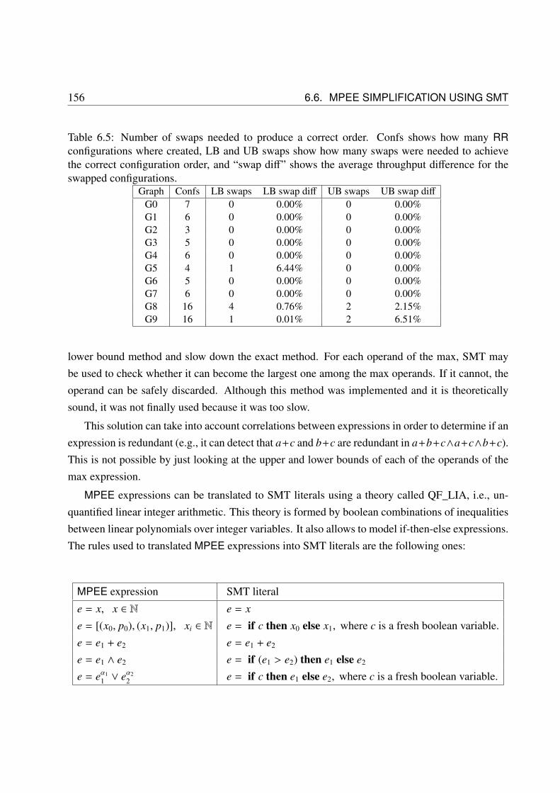
156 6.6. MPEE SIMPLIFICATION USING SMT
Table 6.5: Number of swaps needed to produce a correct order. Confs shows how many RRconfigurations where created, LB and UB swaps show how many swaps were needed to achievethe correct configuration order, and “swap diff” shows the average throughput difference for theswapped configurations.
Graph Confs LB swaps LB swap diff UB swaps UB swap diffG0 7 0 0.00% 0 0.00%G1 6 0 0.00% 0 0.00%G2 3 0 0.00% 0 0.00%G3 5 0 0.00% 0 0.00%G4 6 0 0.00% 0 0.00%G5 4 1 6.44% 0 0.00%G6 5 0 0.00% 0 0.00%G7 6 0 0.00% 0 0.00%G8 16 4 0.76% 2 2.15%G9 16 1 0.01% 2 6.51%
lower bound method and slow down the exact method. For each operand of the max, SMT maybe used to check whether it can become the largest one among the max operands. If it cannot, theoperand can be safely discarded. Although this method was implemented and it is theoreticallysound, it was not finally used because it was too slow.
This solution can take into account correlations between expressions in order to determine if anexpression is redundant (e.g., it can detect that a+c and b+c are redundant in a+b+c∧a+c∧b+c).This is not possible by just looking at the upper and lower bounds of each of the operands of themax expression.
MPEE expressions can be translated to SMT literals using a theory called QF_LIA, i.e., un-quantified linear integer arithmetic. This theory is formed by boolean combinations of inequalitiesbetween linear polynomials over integer variables. It also allows to model if-then-else expressions.The rules used to translated MPEE expressions into SMT literals are the following ones:
MPEE expression SMT literal
e = x, x ∈ N e = x
e = [(x0, p0), (x1, p1)], xi ∈ N e = if c then x0 else x1, where c is a fresh boolean variable.e = e1 + e2 e = e1 + e2
e = e1 ∧ e2 e = if (e1 > e2) then e1 else e2
e = eα11 ∨ eα2
2 e = if c then e1 else e2, where c is a fresh boolean variable.
CHAPTER 6. SYMBOLIC PERFORMANCE ANALYSIS 157
Variable delays are translated to if-then-else expressions where a free boolean variable modelsthat any of the possible delays can be chosen. It can be extended to any number of possible delays,e.g., for three possible delays:
e = if c0 then x0 else (if c1 then x1 else x2)
Addition is directly translated, max is translated to if-then-else where the condition checks whichis the largest delay, and early evaluation is again modeled by a free boolean variables, meaningthat any of the input expressions can be chosen.
When a new max expression is built, it is checked whether some of the operands are redundant.For example, consider a new expression e = e1 ∧ e2 ∧ e3. Then, the following problem is given tothe SMT solver:
Is e1 > e2 and e1 > e3 satisfiable?
If the problem is unsatisfiable, it means that it is impossible that e1 is the greatest of the delays,for any of the possible values of the boolean variables. Therefore, e1 can be dropped, e = e2∧e3. Ifthe problem is satisfiable, then e1 cannot be discarded. The same must be done to decide whetherto discard e2 and e3. Notice that the order in which the sub-expressions are tested is relevant. If e1
is already discarded, the problem that will be solved is the satisfiability of (e2 > e3). It may be thecase that either e1 and e2 can be discarded, but not both at the same time.
This optimization was implemented using an incremental SMT solver [60]. This way, it ispossible to store a context with the already defined clauses and literals, pushing and popping newclauses and variables. However, it was not efficient to solve a new SMT problem for every operandof every new max expression. It did not scale to large unfoldings in complicated marked graphs.
6.7 Conclusion
This chapter has proposed a method to analyze the performance of elastic systems with earlyevaluation and variable-latency units. Two methods have been proposed, an exact method with anexponential time cost, and a simplification which can efficiently compute a lower bound.
All the needed features of elastic systems can be modeled using a Timed Multi-GuardedMarked Graph with Variable-Delay (TGV). In order to evaluate the throughput of a TGV, a timing

158 6.7. CONCLUSION
simulation is performed for a limited number of cycles. First, the TGV is unfolded, and for eachof the transitions in the unfolded graph, a max-plus algebra expression with early evaluation (anMPEE expression) is created in order to formulate the firing time of the transition. The advantageof using symbolic expressions is that some of the correlations due to reconvergent paths can becaptured and factored out.
Finally, all expressions are evaluated in order to evaluate the throughput of the system. Sinceearly evaluation and variable latency are probabilistic, a probability distribution is obtained whenevaluating MPEE expressions. The mean of the distribution is the average firing time of the tran-sition. If the expressions are evaluated taking into account all correlations, the exact firing times,and thus the exact throughput, can be computed. However, exact evaluation has an exponentialworst-case run-time. By ignoring the correlations that have not been captured and removed in theMPEE expression, the throughput can be computed in linear time with respect to the size of theunfolding, but the returned value is not exact, it is a lower bound of the actual throughput.
The length of the timing simulation is determined dynamically. Typically, it is enough to useonce or twice the number of tokens in the TGV in order to converge with enough confidence on thequality of the result. It has been proven that the required length to compute the throughput alwaysconverges.
Results show that it is possible to obtain a tight lower bound of the throughput. The averageerror of the lower bound method is 6.5%. If this is added to the known method to compute an upperbound of the throughput, it means that the effective cycle time is completely bounded. Applied tothe method proposed in the previous chapter, it can help provide more confidence when discardinga configuration: it is possible to safely discard design points whose effective cycle time lowerbound is larger than the effective cycle time upper bound of the best design point found so far(unless it provides a good performance/area trade-off).
As a future research direction, it may be possible to develop methods to further simplify theMPEE expressions using the fact that unfoldings have a repetitive structure. For example, SMTcould be used to discard late inputs in max expressions during the first periods of the unfolding.Then, it may be possible to learn which inputs are redundant and reuse this information to dis-card inputs later, when SMT is too slow because of the depth of the unfolding. Furthermore, thepresented analysis method may be extended to handle module sharing and active anti-tokens.
Furthermore, new approaches should be developed to leverage the fact that the performanceis bounded both ways. The objective could be to reduce the total number of simulations to beperformed at the end of the exploration, and thus the total run-time. Furthermore, it might be

CHAPTER 6. SYMBOLIC PERFORMANCE ANALYSIS 159
possible to increase the diversity of the set of final solutions, providing more trade-off choices tothe designer who is using the tool. For example, if two design points have very similar cycle timeand throughput bounds, one of them may be discarded. This way, the final set of solutions wouldcontain design points that in principle did not look as promising as the discarded ones. However,there would be more heterogeneity in the final pool of solutions, and at the end they might providea more interesting pipeline.

160 6.7. CONCLUSION

Chapter 7
Conclusions
This thesis has presented a set of contributions on the analysis and optimization of synchronouselastic systems. This chapter gathers the conclusions derived from the previous chapters and dis-cusses some research lines opened by this work.
7.1 Contributions
The starting point of this thesis is the novel work in elastic systems [31, 53, 82, 127], which allowsto build latency-insensitive circuits within a conventional clocked synchronous framework. Thesynchronous elastic approach provides several technical advantages, like the ability to cut longwires without affecting the correctness of the design by adding an empty buffer.
This work shows that it is possible to perform design optimization on elastic systems by usingonly simple correct-by-construction local transformations. On top of this idea, an automatedframework has been built to automatically explore the design space unfolded by this simple setof transformations. In particular, this work has shown that it is possible to automatically build apipeline starting from a functional specification of the design.
A fast method to evaluate the throughput of elastic systems is essential in order to enableautomatic exploration. This thesis has also presented a novel method to analyze the throughput ofan elastic system, which can handle early evaluation and variable-latency units.
161

162 7.1. CONTRIBUTIONS
Automatic Exploration of Elastic Pipelines
Elasticity enables new opportunities for system optimization that target the average case perfor-mance. By using early evaluation, the designer can focus on optimizing frequently used and hencecritical parts of the design. Those blocks that are not critical for the overall performance can havea relaxed timing with some extra latency cost. The obtained performance advantage can also beused for saving power.
This work has proposed a framework for automatic exploration of microarchitectures. Thisframework uses simple correct-by-construction transformations, presented in Chapter 3: memorybypass, retiming, multiplexor retiming, recycling, buffer resizing, introduction of early evalua-tion, anti-token insertion, anti-token retiming, anti-token grouping, introduction of variable-latencyunits and sharing of functional units. Many of these transformations are only applicable to elasticsystems, since they modify the latency of computations or communications. Even though theyhave been proposed and used in other works, this thesis puts them together as the ground overwhich the rest of the contributions of this work are built.
After applying any of these transformations, the resulting system is latency equivalent to theoriginal one, i.e., the stream of valid data transmitted at the outputs of the system is the same givenidentical input streams. This property has been verified using model checking for all transforma-tions.
A novel method for introducing speculative execution in elastic systems is covered in Chapter 4.It is performed by applying Shannon decomposition and module sharing to a non-speculative de-sign. Since both transformations are correct-by-construction, functional equivalence is preservedwhen applying speculation. It has been shown that speculation can be used to enhance performanceof interesting design examples such as variable-latency units or resilient designs.
Chapter 5 shows how to build a pipeline of a closed loop system with register files and me-mories by applying a sequence of elastic transformations. Standard bypass and retiming alone arenot sufficient to build such pipelines. This method enables designers to refine a functional modeltowards a cycle-accurate implementation. An automation of this process is proposed, which caneffectively explore the space of possible pipelines and return a design with a near-optimal per-formance. It is also possible to obtain a set of pipelines with different trade-off options betweenperformance and area.
Design space exploration is driven by certain probabilities that describe the workload expectedto be run on the circuit. For a given workload, there is an optimum pipeline depth that delivers the

CHAPTER 7. CONCLUSIONS 163
best possible performance. Thus, specialization of a design can significantly increase its perfor-mance. The examples in Chapter 5 show how different parameters, such as pipeline depth or datahazard probabilities, affect the performance of the system and the optimal structure of the pipeline.
The proposed exploration method relies on the features of elastic circuits. However, at the end itproposes a specific pipeline structure. All pipelines have some level of elasticity implicitly, becausethey must stall for data dependencies, they may allow operations with different possible latencies,etc. A designer may be interested in obtaining the best possible structure for a pipeline but maynot want to pay the cost of elasticizing the whole design. It may be the case that the proposedpipeline is optimal (or near-optimal) in performance independently of whether it is implementedas a synchronous elastic circuit. The method presented in this thesis may effectively be usedthis way. However, only implementation using elastic systems guarantees that the performancepredicted while exploring the design space will be achieved.
Performance Analysis
Chapter 6 proposes a method to analyze the performance of elastic systems with early evaluationand variable-latency units. The method computes a lower bound of the throughput by unfolding amarked graph, deriving symbolic expressions for the firing times of the transitions and evaluatingthem. The accuracy of the lower bound can be incremented by increasing the number of correla-tions taken into account when the expressions are evaluated. The worst case running time when allcorrelations are taken into account is exponential.
Results show that an accurate lower bound of the throughput can be obtained two orders ofmagnitude faster than simulation. If this is added to the known upper bound method, a goodapproximation of the actual throughput can be achieved quickly without running any simulations.A fast method to estimate the performance of an elastic system is important because it allowsto perform microarchitectural exploration without running any simulations, which are too timeconsuming for the presented exploration framework.
7.2 Further Research
This section gives an overview of possible research lines that may be derived from the results ofthis thesis. Some enhancements to the presented method for automatic pipelining are proposed,and the extension of elastic systems in order to support multi-threading is discussed.

164 7.2. FURTHER RESEARCH
Improvements to the Automatic Pipelining Method
In the core of the automatic pipelining algorithm, it lies the retiming and recycling optimizationprocedure, which is modeled as a mixed integer linear programming problem. In this problem,every node is assigned a delay, a latency and an area. However, it would be possible to extend themodel so that nodes can have various delays and latencies.
For example a node representing an adder can have different implementations: a ripple carryadder, a prefix-tree adder, etc., and variable-latency versions of these implementations with bettertiming but higher latency. All these choices would be available during the optimization procedure,so that the best one in timing can be chosen automatically in critical parts of the design, and animplementation with a more relaxed timing and a smaller area is chosen for parts of the design thatare not critical.
Speculation may also be better embedded within the exploration framework. In this work, theexploration method can only identify places where speculative execution can fit in well structurally.However, in order to apply speculation successfully, it must be possible to predict the outcome ofthe computation over which speculation is being applied. Therefore, a designer must indicatewhich choices can be predicted and must provide a scheduler to do so.
Finally, it could be possible to improve the exploration algorithm by using the knowledgeprovided by the lower bound method, as discussed in the conclusions of Chapter 6. Since there isboth an upper bound and a lower bound for each design point, they can be used to prune the set ofinteresting designs or to make it more diverse.
Multi-threading
Elastic systems implement in-order single-threaded pipelines. As a further research direction,elastic systems may be extended to support multi-threading.
There are few studies on automatic pipelining with multi-threading. In [59], a multi-threadedpipeline can be generated from a parameterized in-order pipelining template. In [122], a moregeneral multi-threaded pipelining approach is proposed starting from an initial transactional speci-fication.
The beauty of elastic systems is that they can be modeled using marked graphs, which allowsto have formal performance analysis and optimization methods. The natural extension in order tosupport multi-threading is to use colored Petri nets [83], where each token is assigned a color (i.e.,a thread). Token order must be preserved within the tokens that belong to the same color, but tokens

CHAPTER 7. CONCLUSIONS 165
W R
W R
F1 F2Thread 1Thread 2
Figure 7.1: Possible implementation for elastic multi-threading support. Grey boxes are sharedunits.
with different colors do not have to preserve any kind of order relationship. The current analysisand optimization methods for elastic methods should be extended in order to support colors.
In the simplest approach to implement multi-threaded elastic systems, each thread would own acopy of an automatically generated pipeline. Next, the thread-independent copies may be mergedusing the sharing transformation. Each clock cycle, the scheduler of each shared block woulddecide which thread can use the block. For example, Fig. 7.1 shows a simple pipeline with twothreads. Each thread has its own register file, and the functional units F1 and F2 are shared by thethreads.
This approach is simple and allows total thread scheduling freedom. However, it also has alarge area overhead, since each EB and the whole elastic controller is replicated once per thread.New transformations such as sharing of EBs may alleviate this overhead. A more efficient imple-mentation would consist of adding a color identifier to the handshake protocol of elastic controllers.All the control primitives should be extended and verified accordingly. In particular, there may bedifferent possible versions of EBs depending on whether they allow reordering of tokens with dif-ferent colors (better performance), or they behave strictly as a FIFO (simpler and smaller in area).
Once a performance analysis method is developed for multi-threaded elastic systems, it may bepossible to extend the optimization methods: retiming and recycling, buffer sizing and automaticpipelining methods.

166 7.2. FURTHER RESEARCH

Bibliography
[1] Berkeley Logic Synthesis and Verication Group. ABC: A System for Sequential Synthesisand Verification. http://www-cad.eecs.berkeley.edu/˜alanmi/abc/.
[2] A. Agarwal, D. Blaauw, V. Zolotov, and S. Vrudhula. Computation and refinement of sta-tistical bounds on circuit delay. In Proc. ACM/IEEE Design Automation Conf. (DAC), pages348–353. ACM New York, NY, USA, 2003.
[3] V. Agarwal, M. S. Hrishikesh, S. W. Keckler, and D. Burger. Clock rate versus IPC: the endof the road for conventional microarchitectures. SIGARCH Computer Architecture News,28(2):248–259, 2000.
[4] A. Agiwal and M. Singh. An architecture and a wrapper synthesis approach for multi-clocklatency-insensitive systems. In Proc. Int. Conf. Computer-Aided Design (ICCAD), pages1006–1013, 2005.
[5] M. Akian, R. Bapat, and S. Gaubert. Max-plus algebra. Handbook of Linear algebra:
Discrete Mathematics and its Application, Chapman & Hall/CRC, Baton Rouge, LA, 2007.
[6] M. Ampalam and M. Singh. Counterflow pipelining: Architectural support for preemptionin asynchronous systems using anti-tokens. In Proc. Int. Conf. Computer-Aided Design
(ICCAD), pages 611–618, Nov. 2006.
[7] A. Armando, C. Castellini, and E. Giunchiglia. Sat-based procedures for temporal rea-soning. In ECP ’99: Proc. European Conf. Planning, pages 97–108, London, UK, 2000.Springer-Verlag.
[8] P. Ashar, S. Devadas, and A. Newton. Sequential logic synthesis. Springer, 1992.
167

168 BIBLIOGRAPHY
[9] D. Bañeres, J. Cortadella, and M. Kishinevsky. Variable-latency design by function spec-ulation. In Proc. Design, Automation and Test in Europe (DATE), pages 1704–1709, Mar.2009.
[10] P. Beerel, A. Lines, M. Davies, and N. Kim. Slack matching asynchronous designs. In Proc.
Int. Symp. Asynchronous Circuits and Systems, page 11, 2006.
[11] L. Benini, E. Macii, and M. Poncino. Telescopic units: increasing the average throughputof pipelined designs by adaptive latency control. In Proc. ACM/IEEE Design Automation
Conf. (DAC), pages 22–27, 1997.
[12] L. Benini, G. D. Micheli, A. Lioy, E. Macii, G. Odasso, and M. Poncino. Automatic syn-thesis of large telescopic units based on near-minimum timed supersetting. IEEE Trans. on
Computers, 48(8):769–779, 1999.
[13] K. Bernstein, D. Frank, A. Gattiker, W. Haensch, B. Ji, S. Nassif, E. Nowak, D. Pearson,and N. Rohrer. High-performance CMOS variability in the 65-nm regime and beyond. IBM
Journal of Research and Development, 50(4/5):449, 2006.
[14] C. Berthet, O. Coudert, and J. C. Madre. New Ideas on Symbolic Manipulations of FiniteState Machines. In Proc. Int. Conf. Computer-Aided Design (ICCAD), pages 224–227, 1990.
[15] E. Best. Structure theory of Petri nets: the free choice hiatus. Petri Nets: Central Models
and Their Properties, pages 168–205, 1987.
[16] E. Bloch. The engineering design of the stretch computer. In Proc. IRE/AIEE/ACM Eastern
Joint Computer Conference, pages 48–58, Dec. 1959.
[17] S. Borkar. Design challenges of technology scaling. IEEE Micro, 19(4):23–29, 1999.
[18] S. Borkar. Thousand core chips: a technology perspective. In Proc. ACM/IEEE Design
Automation Conf. (DAC), pages 746–749, 2007.
[19] J. Boucaron, R. de Simone, and J. Millo. Latency-insensitive design and central repeti-tive scheduling. In Proc. ACM/IEEE Int. Conf. Formal Methods and Models for Codesign
(MEMOCODE), pages 175–183. IEEE, 2006.

BIBLIOGRAPHY 169
[20] A. Branover, R. Kol, and R. Ginosar. Asynchronous design by conversion: convertingsynchronous circuits into asynchronous ones. In Proc. Design, Automation and Test in
Europe (DATE), volume 2, pages 870–875, 2004.
[21] C. Brej. Early Output Logic and Anti-Tokens. PhD thesis, University of Manchester, 2005.
[22] R. Bryant. Binary decision diagrams and beyond: Enabling technologies for formal verifi-cation. In Proc. ACM/IEEE Design Automation Conf. (DAC), pages 236–243, 1995.
[23] D. Bufistov. Performance Optimization of Elastic Systems. PhD thesis, Universitat Politec-nica de Catalunya, 2010.
[24] D. Bufistov, J. Cortadella, M. Galceran-Oms, J. Júlvez, and M. Kishinevsky. Retiming andrecycling for elastic systems with early evaluation. In Proc. ACM/IEEE Design Automation
Conf. (DAC), pages 288–291, July 2009.
[25] D. Bufistov, J. Cortadella, M. Galceran-Oms, J. Júlvez, and M. Kishinevsky.Retiming and recycling for elastic systems with early evaluation. (available athttp://www.lsi.upc.edu/dept/techreps/llistat_detallat.php?id=1050). Technical report, 2009.
[26] D. Bufistov, J. Cortadella, M. Kishinevsky, and S. Sapatnekar. A general model for per-formance optimization of sequential systems. In Proc. Int. Conf. Computer-Aided Design
(ICCAD), pages 362–369, 2007.
[27] D. Bufistov, J. Júlvez, and J. Cortadella. Performance optimization of elastic systems usingbuffer resizing and buffer insertion. In Proc. Int. Conf. Computer-Aided Design (ICCAD),pages 442–448, Nov. 2008.
[28] S. Burns. Performance analysis and optimization of asynchronous circuits. PhD thesis,California Institute of Technology, 1990.
[29] J. Campos, G. Chiola, J. Colom, and M. Silva. Tight polynomial bounds for steady-state per-formance of marked graphs. In Workshop on Petri Nets and Performance Models, (PNPM),pages 200–209, 1989.
[30] J. Campos, G. Chiola, and M. Silva. Ergodicity and throughput bounds of Petri nets withunique consistent firing count vector. IEEE Trans. on Software Engineering, 17(2):117–125,1991.

170 BIBLIOGRAPHY
[31] L. Carloni, K. McMillan, A. Saldanha, and A. Sangiovanni-Vincentelli. A methodologyfor correct-by-construction latency insensitive design. In Proc. Int. Conf. Computer-Aided
Design (ICCAD), pages 309–315. IEEE Press, Nov. 1999.
[32] L. Carloni, K. McMillan, and A. Sangiovanni-Vincentelli. Theory of latency-insensitivedesign. IEEE Trans. Computer-Aided Design, 20(9):1059–1076, Sept. 2001.
[33] L. Carloni and A. Sangiovanni-Vincentelli. Performance analysis and optimization of la-tency insensitive systems. In Proc. ACM/IEEE Design Automation Conf. (DAC), page 367,2000.
[34] L. Carloni and A. Sangiovanni-Vincentelli. Coping with latency in SoC design. IEEE Micro,
Special Issue on Systems on Chip, 22(5):12, October 2002.
[35] L. Carloni and A. Sangiovanni-Vincentelli. Combining retiming and recycling to optimizethe performance of synchronous circuits. In 16th Symp. on Integrated Circuits and System
Design (SBCCI), pages 47–52, Sept. 2003.
[36] J. Carmona, J. Cortadella, M. Kishinevsky, and A. Taubin. Elastic circuits. IEEE Trans. on
Computer-Aided Design, 28(10):1437–1455, Oct. 2009.
[37] J. Carmona, J. Júlvez, J. Cortadella, and M. Kishinevsky. Scheduling Synchronous ElasticDesigns. In Conf. Application of Concurrency to System Design (ACSD), pages 52–59.IEEE, 2009.
[38] M. Casu. Improving synchronous elastic circuits: Token cages and half-buffer retiming. InProc. Int. Symp. Asynchronous Circuits and Systems, pages 128–137, 2010.
[39] M. Casu and L. Macchiarulo. A new approach to latency insensitive design. In Proc.
ACM/IEEE Design Automation Conf. (DAC), pages 576–581, June 2004.
[40] M. Casu and L. Macchiarulo. Adaptive Latency-Insensitive Protocols. IEEE Design & Test
of Computers, 24(5):442–452, 2007.
[41] M. Casu and L. Macchiarulo. Adaptive Latency Insensitive Protocols and Elastic Circuitswith Early Evaluation: A Comparative Analysis. Electronic Notes in Theoretical Computer
Science, 245:35–50, 2009.

BIBLIOGRAPHY 171
[42] S. Chakraborty, K. Yun, and D. Dill. Timing analysis of asynchronous systems using timeseparation of events. IEEE transactions on computer-aided design of integrated circuits and
systems, 18(8):1061–1076, 1999.
[43] T. Chelcea and S. Nowick. Robust interfaces for mixed-timing systems. IEEE Trans. VLSI
Syst., 12(8):857–873, 2004.
[44] A. Cimatti, E. Clarke, E. Giunchiglia, F. Giunchiglia, M. Pistore, M. Roveri, R. Sebastiani,and A. Tacchella. Nusmv 2: An opensource tool for symbolic model checking. Lecture
Notes in Computer Science, pages 359–364, 2002.
[45] R. Collins and L. P. Carloni. Topology-based optimization of maximal sustainable through-put in a latency-insensitive system. In Proc. ACM/IEEE Design Automation Conf. (DAC),pages 410–416, June 2007.
[46] M. Comeau and K. Thulasiraman. Structure of the Submarking-Reachability Problem andNetwork Programming. IEEE Trans. on Circuits and Systems, 35(1), 1988.
[47] J. Cong. Challenges and opportunities for design innovations in nanometer technologies.Invited Semiconductor Research Corporation Design Sciences Concept Paper, pages 1–15,may 1998.
[48] J. Cortadella, M. Galceran-Oms, and M. Kishinevsky. Elastic systems. In Proc. ACM/IEEE
Int. Conf. Formal Methods and Models for Codesign (MEMOCODE), pages 149–158, July2010.
[49] J. Cortadella and M. Kishinevsky. Synchronous elastic circuits with early evaluation andtoken counterflow. In Proc. ACM/IEEE Design Automation Conf. (DAC), pages 416–419,June 2007.
[50] J. Cortadella and M. Kishinevsky. Synchronous elastic circuits with early eva-luation and token counterflow. (available at http://www.lsi.upc.edu/dept/techreps/ llis-tat_detallat.php?id=958). Technical report, 2007.
[51] J. Cortadella, M. Kishinevsky, D. Bufistov, J. Carmona, and J. Júlvez. Elasticity and PetriNets. Trans. on Petri Nets and Other Models of Concurrency I, 5100:221–249, Aug. 2008.

172 BIBLIOGRAPHY
[52] J. Cortadella, M. Kishinevsky, and B. Grundmann. SELF: Specification and design of asynchronous elastic architecture for DSM systems. In TAU-2006: Int. Workshop on Timing
Issues in the Specification and Synthesis of Digital Systems, 2006.
[53] J. Cortadella, M. Kishinevsky, and B. Grundmann. Synthesis of synchronous elastic archi-tectures. In Proc. ACM/IEEE Design Automation Conf. (DAC), pages 657–662, July 2006.
[54] J. Cortadella, A. Kondratyev, L. Lavagno, and C. Sotiriou. Desynchronization: Synthesisof asynchronous circuits from synchronous specifications. IEEE Trans. Computer-Aided
Design of Integrated Circuits and Systems, 25(10):1904–1921, 2006.
[55] I. CPLEX. 10.0 user’s manual. ILOG SA, Gentilly, France, 2005.
[56] G. Dantzig. Linear Programming and Extensions. 1963.
[57] A. Dasdan, S. Irani, and R. Gupta. Efficient algorithms for optimum cycle mean and op-timum cost to time ratio problems. In Proc. ACM/IEEE Design Automation Conf. (DAC),page 42. ACM, 1999.
[58] G. De Micheli. Synthesis and optimization of digital circuits. McGraw-Hill Higher Educa-tion, 1994.
[59] R. Dimond, O. Mencer, and W. Luk. Application-specific customisation of multi-threadedsoft processors. In IEEE Proc. Computers and Digital Techniques, volume 153, pages 173–180. IET, 2006.
[60] B. Dutertre and L. De Moura. The yices smt solver. Tool paper at http://yices. csl. sri.
com/tool-paper. pdf, 2006.
[61] J. Esparza and K. Heljanko. Unfoldings: a partial-order approach to model checking.Springer-Verlag, 2008.
[62] S. Eyerman, L. Eeckhout, and K. De Bosschere. Efficient design space exploration of highperformance embedded out-of-order processors. In Proc. Design, Automation and Test in
Europe (DATE), pages 351–356, 2006.
[63] M. Galceran-Oms, J. Cortadella, and M. Kishinevsky. Symbolic performance analysis ofelastic systems. In Proc. Int. Conf. Computer-Aided Design (ICCAD), pages 778–785. IEEE.
BIBLIOGRAPHY 173
[64] M. Galceran-Oms, J. Cortadella, and M. Kishinevsky. Speculation in elastic systems. InProc. ACM/IEEE Design Automation Conf. (DAC), pages 292–295, July 2009.
[65] M. Galceran-Oms, J. Cortadella, M. Kishinevsky, and D. Bufistov. Automatic microarchi-tectural pipelining. In Proc. Int. Workshop on Logic Synthesis, pages 214–221, June 2009.
[66] M. Galceran-Oms, J. Cortadella, M. Kishinevsky, and D. Bufistov. Automatic microarchi-tectural pipelining. In Proc. Design, Automation and Test in Europe (DATE), pages 961–964,Mar. 2010.
[67] G. Gill, V. Gupta, and M. Singh. Performance estimation and slack matching for pipelinedasynchronous architectures with choice. In Proc. Int. Conf. Computer-Aided Design (IC-
CAD), pages 449–456, 2008.
[68] A. Gotmanov, M. Kishinevsky, and M. Galceran-Oms. Evaluation of flexible latencies:designing synchronous elastic H.264 CABAC decoder. In In Proc. of the Problems in design
of micro- and nano-electronic systems (in Russian), Oct. 2010.
[69] P. L. Guernic, J.-P. Talpin, and J.-C. L. Lann. Polychrony for system design. Journal of
Circuits, Systems and Computers, 12(3):261–304, Apr. 2003.
[70] J. Gunawardena. Timing analysis of digital circuits and the theory of min-max functions. InTAU’93, ACM Int. Workshop on Timing Issues in the Specification and Synthesis of Digital
Systems, 1993.
[71] G. Hachtel and F. Somenzi. Logic synthesis and verification algorithms. Kluwer AcademicPub, 1996.
[72] A. Hartstein and T. R. Puzak. The optimum pipeline depth for a microprocessor. In Proc.
Int. Symp. Computer Architecture, pages 7–13, 2002.
[73] S. Hassoun and C. Ebeling. Architectural retiming: Pipelining latency-constrained circuits.In Proc. ACM/IEEE Design Automation Conf. (DAC), pages 708–713, June 1996.
[74] S. Hassoun and C. Ebeling. Using precomputation in architecture and logic resynthesis. InProc. Int. Conf. Computer-Aided Design (ICCAD), pages 316–323, 1998.

174 BIBLIOGRAPHY
[75] J. Hennessy and D. Patterson. Computer Architecture: a Quantitative Approach. MorganKaufmann Publisher Inc., 1990.
[76] J. Higgins and M. Aagaard. Simplifying the design and automating the verification ofpipelines with structural hazards. ACM Trans. Design Automation of Electronic Systems
(TODAES), 10(4):672, 2005.
[77] J. Hoe and Arvind. Synthesis of operation-centric hardware descriptions. In Proc. Int. Conf.
Computer-Aided Design (ICCAD), pages 511–519. IEEE Press Piscataway, NJ, USA, 2000.
[78] G. Hoover and F. Brewer. Synthesizing synchronous elastic flow networks. In Proc. Design,
Automation and Test in Europe (DATE), pages 306–311. ACM, 2008.
[79] M. Hrishikesh, N. Jouppi, K. Farkas, D. Burger, S. Keckler, and P. Shivakumar. The optimallogic depth per pipeline stage is 6 to 8 FO4 inverter delays. ACM SIGARCH Computer
Arch., 30(2):14–24, 2002.
[80] H. Hulgaard, S. Burns, T. Amon, and G. Borriello. An algorithm for exact bounds onthe time separation of events in concurrent systems. IEEE transactions on computers,44(11):1306–1317, 1995.
[81] A. P. Hurst, A. Mishchenko, and R. K. Brayton. Scalable min-register retiming under timingand initializability constraints. In Proc. ACM/IEEE Design Automation Conf. (DAC), pages534–539, June 2008.
[82] H. M. Jacobson, P. N. Kudva, P. Bose, P. W. Cook, S. E. Schuster, E. G. Mercer, and C. J.Myers. Synchronous interlocked pipelines. In Proc. Int. Symp. Asynchronous Circuits and
Systems, pages 3–12, Apr. 2002.
[83] K. Jensen. Coloured Petri nets: basic concepts, analysis methods and practical use.Springer-Verlag, 1997.
[84] A. Jerraya. Long term trends for embedded system design. In Proc. CEPA 2 Workshop,2005.
[85] J. Júlvez, J. Cortadella, and M. Kishinevsky. Performance analysis of concurrent systemswith early evaluation. In Proc. Int. Conf. Computer-Aided Design (ICCAD), Nov. 2006.

BIBLIOGRAPHY 175
[86] J. Júlvez, J. Cortadella, and M. Kishinevsky. On the performance evaluation of multi-guarded marked graphs with single-server semantics. Discrete Event Dynamic Systems,20(3):377–407, Sept. 2010.
[87] T. Kam, M. Kishinevsky, J. Cortadella, and M. Galceran-Oms. Correct-by-constructionmicroarchitectural pipelining. In Proc. Int. Conf. Computer-Aided Design (ICCAD), pages434–441, 2008.
[88] N. Karmarkar. A new polynomial-time algorithm for linear programming. Combinatorica,4(4):373–396, 1984.
[89] R. Karp. A characterization of the minimum mean-cycle in a digraph. Discrete Maths,23:309–311, 1978.
[90] L. Khachiyan. A polynomial algorithm for linear programming (Russian). In Doklady
Akademii Nauk SSSR 244, pages 1093–1096, 1979.
[91] E. Kilada and K. Stevens. Control Network Generator For Latency Insensitive Designs. InProc. Design, Automation and Test in Europe (DATE), Apr. 2010.
[92] M. Kishinevsky, A. Kondratyev, A. Taubin, and V. Varshavsky. Concurrent hardware: the
theory and practice of self-timed design. John Wiley & Sons, Inc., 1994.
[93] R. Kol and R. Ginosar. A doubly-latched asynchronous pipeline. In Proc. IEEE Int. Conf.
Computer Design: VLSI in Computers and Processors (ICCD), pages 706–711, 1997.
[94] Y. Kondo, N. Ikumi, K. Ueno, J. Mori, and M. Hirano. An early-completion-detecting ALUfor a 1 GHz 64b datapath. In IEEE Int. Conf. Solid-State Circuits (ISSCC), pages 418–419,1997.
[95] D. Kroening and W. Paul. Automated pipeline design. In Proc. ACM/IEEE Design Automa-
tion Conf. (DAC), pages 810–815, 2001.
[96] S. Krstic, J. Cortadella, M. Kishinevsky, and J. O’Leary. Synchronous elastic networks. InInt. Conf. on Formal Methods in Computer-Aided Design (FMCAD), Nov. 2006.
[97] P. Kudva, G. Gopalakrishnan, E. Brunvand, and V. Akella. Performance Analysis and Op-timization of Asynchronous Circuits. In Proc. IEEE Int. Conf. Computer Design: VLSI in
Computer & Processors, pages 221–224, 1994.

176 BIBLIOGRAPHY
[98] C. E. Leiserson and J. B. Saxe. Retiming synchronous circuitry. Algorithmica, 6(1):5–35,1991.
[99] C.-H. Li and L. Carloni. Using functional independence conditions to optimize the perfor-mance of latency-insensitive systems. In Proc. Int. Conf. Computer-Aided Design (ICCAD),Nov. 2007.
[100] C.-H. Li, R. Collins, S. Sonalkar, and L. P. Carloni. Design, implementation, and validationof a new class of interface circuits for latency-insensitive design. In Proc. ACM/IEEE Int.
Conf. Formal Methods and Models for Codesign (MEMOCODE), pages 13–22, 2007.
[101] J. Liou, K. Cheng, S. Kundu, and A. Krstic. Fast statistical timing analysis by probabilisticevent propagation. In Proc. ACM/IEEE Design Automation Conf. (DAC), pages 661–666,2001.
[102] R. Lu and C. Koh. Performance analysis of latency-insensitive systems. IEEE Trans.
Computer-Aided Design of Integrated Circuits and Systems, 25(3):469–483, 2006.
[103] R. Lu and C.-K. Koh. Performance optimization of latency insensitive systems throughbuffer queue sizing of communication channels. In Proc. Int. Conf. Computer-Aided Design
(ICCAD), pages 227–231, Nov. 2003.
[104] R. Manohar and A. Martin. Slack elasticity in concurrent computing. In Mathematics of
Program Construction, pages 272–285. Springer, 1998.
[105] M.-C. V. Marinescu and M. C. Rinard. High-level automatic pipelining for sequential cir-cuits. In Proc. Int. Symp. on Systems Synthesis, pages 215–220, 2001.
[106] J. Matthews and J. Launchbury. Elementary microarchitecture algebra. Lecture Notes in
Computer Science, 1633:288–300, 1999.
[107] K. McMillan. Using unfoldings to avoid the state explosion problem in the verification ofasynchronous circuits. In Computer Aided Verification, pages 164–177, 1992.
[108] K. McMillan. Verification of infinite state systems by compositional model checking. Cor-
rect Hardware Design and Verification Methods, 1703:219–237, 1999.

BIBLIOGRAPHY 177
[109] K. L. McMillan. A compositional rule for hardware design refinement. In Computer Aided
Verification, pages 24–35. Springer, 1997.
[110] E. Mercer and C. Myers. Stochastic cycle period analysis in timed circuits. In IEEE Int.
Symp. Circuits and Systems (ISCAS), volume 2, pages 172–175, 2000.
[111] P. Mishra, A. Kejariwal, and N. Dutt. Synthesis-driven exploration of pipelined embeddedprocessors. In Proc. Int. Conf. VLSI Design, pages 921–926, 2004.
[112] D. Misunas. Petri nets and speed independent design. Communications of the ACM,16(8):481, 1973.
[113] J. Monteiro, S. Devadas, and A. Ghosh. Retiming sequential circuits for low power. InProc. Int. Conf. Computer-Aided Design (ICCAD), pages 398–402, 1993.
[114] G. Moore. Cramming more components onto integrated circuits. 38(8):114–117, Apr. 1965.
[115] T. Murata. Petri Nets: Properties, analysis and applications. Proc. of the IEEE, pages541–580, Apr. 1989.
[116] K. G. Murty. Linear Programming. Wiley and Sons, 1983.
[117] S. R. Nassif. Design for variability in dsm technologies. In Proc. Int. Symp. Quality of
Electronic Design (ISQED), pages 451–454, 2000.
[118] C. Nielsen and M. Kishinevsky. Performance analysis based on timing simulation. In Proc.
ACM/IEEE Design Automation Conf. (DAC), pages 70–76, 1994.
[119] M. Nielsen, G. Plotkin, and G. Winskel. Petri nets, event structures and domains, part I.Theoretical Computer Science, 13(1):85–108, 1981.
[120] R. Nieuwenhuis, A. Oliveras, and C. Tinelli. Solving SAT and SAT Modulo Theories:From an abstract Davis–Putnam–Logemann–Loveland procedure to DPLL (T). Journal of
the ACM (JACM), 53(6):977, 2006.
[121] E. Nurvitadhi, J. Hoe, T. Kam, and S. Lu. Automatic Pipelining from Transactional DatapathSpecifications. Proc. Design, Automation and Test in Europe (DATE), pages 1001–1004,Mar. 2010.

178 BIBLIOGRAPHY
[122] E. Nurvitadhi, J. Hoe, S. Lu, and T. Kam. Automatic multithreaded pipeline synthesis fromtransactional datapath specifications. In Proc. ACM/IEEE Design Automation Conf. (DAC),pages 314–319, 2010.
[123] J. O’Leary and G. Brown. Synchronous emulation of asynchronous circuits. IEEE Trans.
Computer-Aided Design of Integrated Circuits and Systems, 16(2):205–209, 2002.
[124] K. Olukotun and L. Hammond. The future of microprocessors. Queue, 3(7):26–29, 2005.
[125] C. Papadimitriou. Computational Complexity. Addison-Wesley, 1995.
[126] N. Park and A. Parker. Sehwa: a software package for synthesis of pipelines frombehavioralspecifications. IEEE Trans. Computer-Aided Design of Integrated Circuits and Systems,7(3):356–370, 1988.
[127] A. Peeters and K. Van Berkel. Synchronous handshake circuits. In Proc. Int. Symp. Ad-
vanced Research in Asynchronous Circuits and Systems, pages 86–95, March 2001.
[128] A. Pnueli. The temporal logic of programs. In Proc. IEEE Symp. Foundations of Computer
Science, pages 46–57, 1977.
[129] M. D. Powell, A. Biswas, J. S. Emer, S. S. Mukherjee, B. R. Sheikh, and S. Yardi. CAMP:A technique to estimate per-structure power at run-time using a few simple parameters. InIEEE Int. Symp. High Performance Computer Architecture (HPCA), pages 289–300, Feb.2009.
[130] P. Prakash and A. Martin. Slack matching quasi delay-insensitive circuits. In Proc. Int.
Symp. Asynchronous Circuits and Systems, page 10, 2006.
[131] C. Ramamoorthy and G. Ho. Performance Evaluation of Asynchronous Concurrent SystemsUsing Petri Nets. IEEE Trans. on Software Engineering, 6(5):440–449, 1980.
[132] C. Ramchandani. Analysis of asynchronous concurrent systems by timed petri nets. Tech-nical report, Project MAC, TR-120, MIT, 1974.
[133] R. Reese, M. Thornton, and C. Traver. A coarse-grain phased logic cpu. IEEE Trans.
Comput., 54:788–799, July 2005.

BIBLIOGRAPHY 179
[134] R. Reese, M. Thornton, C. Traver, and D. Hemmendinger. Early evaluation for performanceenhancement in phased logic. IEEE Trans. Computer-Aided Design, 24(4):532–550, Apr.2005.
[135] J. Rodriguez-Beltran and A. Ramfrez-Trevino. Minimum initial marking in timed markedgraphs. In IEEE Int. Conf. Systems, Man, and Cybernetics, volume 4, pages 3004–3008,2000.
[136] S. S. Sapatnekar. Timing. Kluwer Academic Publishers, 2004.
[137] S. S. Sapatnekar and R. B. Deokar. Utilizing the timing skew equivalence in a practicalalgorithm for retiming large circuits. IEEE Trans. Computer-Aided Design, 15(10):1237–1248, Oct. 1996.
[138] P. Saxena, N. Menezes, P. Cocchini, and D. Kirkpatrick. Repeater scaling and its impacton CAD. IEEE Trans. on Computer-Aided Design of Integrated Circuits and Systems,23(4):451–463, 2004.
[139] E. Sentovich, K. Singh, L. Lavagno, C. Moon, R. Murgai, A. Saldanha, H. Savoj, P. Stephan,R. Brayton, and A. Sangiovanni-Vincentelli. SIS: A System for Sequential Circuit SynthesisUniversity of California at Berkeley. UCB/ERL M, 1992.
[140] J. Shen and M. Lipasti. Modern processor design: fundamentals of superscalar processors.McGraw-Hill Science Engineering, 2004.
[141] N. V. Shenoy. Retiming: Theory and practice. Integration, the VLSI Journal, 22(1):1–21,1997.
[142] M. Silva. Introducing petri nets. Practice of Petri Nets in Manufacturing, pages 1–62, 1993.
[143] M. Singh and M. Theobald. Generalized latency-insensitive systems for single-clock andmulti-clock architectures. In Proc. Design, Automation and Test in Europe (DATE), page21008, 2004.
[144] C. Soviani, O. Tardieu, and S. Edwards. Optimizing sequential cycles through Shannondecomposition and retiming. In Proc. Design, Automation and Test in Europe (DATE),pages 1085–1090, 2006.

180 BIBLIOGRAPHY
[145] L. Spracklen and S. Abraham. Chip multithreading: Opportunities and challenges. In Proc.
Int. Symp. High-Performance Computer Architecture, pages 248–252, 2005.
[146] S. Srinivasan, K. Sarker, and R. Katti. Token-Aware Completion Functions for Elastic Pro-cessor Verification. Research Letters in Electronics, 2009.
[147] Y.-S. Su, D.-C. Wang, S.-C. Chang, and M. Marek-Sadowska. An efficient mechanism forperformance optimization of variable-latency designs. In Proc. ACM/IEEE Design Automa-
tion Conf. (DAC), pages 976–981, 2007.
[148] S. Suhaib, D. Mathaikutty, D. Berner, and S. Shukla. Validating families of latency insensi-tive protocols. IEEE Trans. Comput., 55:1391–1401, November 2006.
[149] I. E. Sutherland. Micropipelines. Communications of the ACM, 32(6):720–738, June 1989.
[150] H. J. Touati and R. K. Brayton. Computing the initial states of retimed circuits. IEEE Trans.
on CAD of Integrated Circuits and Systems, 12(1):157–162, 1993.
[151] V. Varshavsky and V. Marakhovsky. GALA (Globally Asynchronous: Locally Arbitrary)Design. Concurrency and Hardware Design, pages 61–107, 2002.
[152] M. Vijayaraghavan and Arvind. Bounded dataflow networks and latency-insensitive circuits.In Proc. ACM/IEEE Int. Conf. Formal Methods and Models for Codesign (MEMOCODE),July 2009.
[153] J. Wakerly, C. Jong, and C. Chang. Digital Design: Principles and Practices. Prentice HallEnglewood Cliffs, NJ, 2001.
[154] T. Williams. Performance of iterative computation in self-timed rings. The Journal of VLSI
Signal Processing, 7(1):17–31, 1994.
[155] R. W. Wolff. Stochastic modeling and the theory of queues. Prentice Hall, 1989.
[156] A. Xie and P. Beerel. Symbolic techniques for performance analysis of timed systems basedon average time separation of events. In Int. Symp. Advanced Research in Asynchronous
Circuits and Systems, pages 64–75, 1997.
[157] A. Xie and P. Beerel. Performance analysis of asynchronous circuits and systems usingstochastic timed Petri nets. In Hardware Design and Petri Nets, 1999.

BIBLIOGRAPHY 181
[158] Xilinx. Single Error Correction and Double Error Detection (SECDED) with CoolRunner-IICPLDs. Application Note XAPP383, 1:1–4, 2003.
[159] A. Yakovlev, M. Kishinevsky, A. Kondratyev, L. Lavagno, and M. Pietkiewicz-Koutny. Onthe models for asynchronous circuit behaviour with or causality. Formal Methods in System
Design, 9:189–233, 1996.

Index
SELF protocol, 21, 30
adaptive latency-insensitive designs, 28anti-tokens, 28, 63, 64, 75, 94, 95, 114, 125asynchronous designs, 5
backpressure, 19, 21, 58, 125bubble insertion, 57, 74, 94buffer capacity, 58bypass, 54, 88, 95
correct-by-construction, 10, 49, 69, 73, 89critical core, 61, 113cycle time, 2, 21
data hazard, 92, 96data variability, 61deadlock, 58, 69
early evaluation, 28, 54, 60, 73, 75, 78, 88, 94,119, 124, 130
effective cycle time, 21elastic buffers, 19, 22, 31, 69, 78elastic channel, 19elastic marked graph, 41elastic module, 18error correction, 80
fork, 26, 33functional independence conditions, 28
granularity, 37
infinite-server semantics, 16, 104, 127integer linear programming, 17, 59, 94, 106
join, 26, 33
latency-insensitive designs, 18linear programming, 17, 45little care, 61, 113
MAREX, 53, 102marked graph, 16, 41, 117, 124Markov chain, 45, 89microarchitectural graph, 51, 94mixed integer linear programming, 59module sharing, 67, 69, 77multiplexor, 54multiplexor retiming, 57
NuSMV, 53
Petri net, 15, 41, 126pipeline, 3pipelining, 11, 46, 87, 88, 92, 99, 103, 109
recycling, 57, 94register file, 40, 52retiming, 56, 94retiming and recycling, 58, 94
182

INDEX 183
scheduling, 37single-server semantics, 16, 125, 127skid-buffer, 25, 58slack matching, 58speculation, 11, 73synchronous designs, 2synthesis flow, 39, 50
throughput, 17, 20, 127, 151timed marked graph, 16, 41, 124toolkit, 53transfer equivalence, 20, 69transformations, 10, 49
unfolding, 126, 146
variable-latency, 52, 66, 82, 118, 125, 130verification, 35, 69Verilog, 53video decoder, 62, 113


![Pipelining & Parallel Processing - ics.kaist.ac.krics.kaist.ac.kr/ee878_2018f/[EE878]3 Pipelining and Parallel Processing.pdf · Pipelining processing By using pipelining latches](https://img.dokumen.tips/doc/110x75/5d40e26d88c99391748d47fb/pipelining-parallel-processing-icskaistackricskaistackree8782018fee8783.jpg)