Automatic Image Mosaic System Using Image FeatureDetection and Taylor Series

Soo-Hyun CHO , Yun-Koo CHUNG, Jae Yeon LEE

161 Gajeong-dong, Yuseong-gu, Daejeon, 305-350 KOREAElectronics and Telecommunications Research Institute

Jsh62860@etri.re.kr

Abstract. Image mosaicing has been collecting considerable attention in thefield of computer vision and photogrammetry. Unlike previous methods using atripod, we have developed which can handle images taken with a hand-heldcamera to accurately construct a panoramic image. This paper proposes theautomatic image mosaic system implementation, which it sees to use featuredetection of the image, which is extracted a feature point adjustment fromcontinuous two images hour automatically from pixel price of image and inorder to accomplish. Feature based image mosaics require the integration ofcorner detection, corner matching, motion parameters estimation, and imagestitching. We used Taylor series for parameter and perspective transformestimation.

1. Introduction

In the last few years the interest in mosaicing has grown in the vision communitybecause of its many applications. The automatic construction of large and high-resolution image mosaics is an active area of research in the fields ofphotogrammetry, computer vision, image processing, medical image, real rendering,robot -vision and computer graphics. Image mosaics involve aligning a sequence ofimage into a larger image and are an important issue in many virtual reality problems.Mosaicing is a common and popular method of effectively increasing the field ofview of a camera, by allowing several views of a scene to be combined into singleview. The traditional approach, which uses correlation intensity based [1][2] imageregistration, suffers from computation inefficiency and is sensitive to variations inimage intensity. To improve the efficiency of image mosaics, we used a feature-basedapproach. Two images belonging to a planar scene are related by an affinetransformation and perspective transformation using Taylor series. One of the imagesis used as the reference image, and the second image is aligned with the referenceimage. To find the coordinate transformation between the two images, we firstconduct corner detection to find the corners in these two images. Next, we perform acorner matching process to find the corresponding corner points between these twoimages. We used SSD (Sum of Squared Difference) method for corner matching.After initial matching, in order to remove mismatches corresponding point, which

549

Proc. VIIth Digital Image Computing: Techniques and Applications, Sun C., Talbot H., Ourselin S. and Adriaansen T. (Eds.), 10-12 Dec. 2003, Sydney

does a filtering processing from each image. We can estimate the transformationparameters using the Taylor series. System flowchart is shown in Fig 1. In the nextsection, we give implementation and algorithm of the system and experimental andresults. Finally, conclusions are given in section 4

Fig. 1. Flowchart of Mosaic create system

2. System Implementation and Algorithm

2-1 Image Acquisition

In this paper, we used hand-held camera. The set may consist of two images taken ofscene at different times, from different viewpoints. It is possible that all movements ofcamera, (i.e. pan, tilt, rotation, translation, scale, shear). Outside scene the imagewhich it requires from the of course inside scene is possible. First, if image involvesmore than one band, say RGB, it will be converted to gray-scale image eq. (1). That isI’() is formulate as follow. The reference image and add image of original images areshown in Fig.2

(a) Reference Image (b) Add Image

Fig. 2. Reference image and Add image of test image

bluegreenred yxIyxIyxIyxI ),(114.0),(587.0),(2999.0),(' ×+×+×= (1)

Gray scale conversion Corner detection

Corner detectionGray scale conversionReference Image

Add Image

Initial corner point matchingFiltering of mismatch corner point

Parameter calculation and interpolation Mosaic Image

550

Proc. VIIth Digital Image Computing: Techniques and Applications, Sun C., Talbot H., Ourselin S. and Adriaansen T. (Eds.), 10-12 Dec. 2003, Sydney

P(x,y)q(x,y)

w

2-2 Corner detection using SUSAN method

In this approach, we first detect corner points using the SUSAN(Smallest UnivauleSegment Assimilating Nucleus) principle in the each two images [3]. The response isprocessed to output the set of corners. The mask is places at each in the image and, foreach point, the brightness of each pixel within the mask is compared with that of the

nucleus, i.e. the center point. The comparison uses the eq.(2) here , 0rr

is the position

of nucleus,rr

position of an other point within the mask,)(rI

r

the brightness of anypixel, t the brightness difference threshold and c the output. With figure 3,Considering 7×7 pixel region window (w) that point in the center and optional pointp(x, y) in the image, from inside the w different one point q(x, y) it does. I(p) and I(q)shows intensity values each point from p and q. Calculate the number of pixels withinthe circular mask which have similar brightness to the nucleus. Input image is grayscale value, T the brightness difference threshold and G the Gaussian value eq(3)

(a) (b)

Fig. 3. SUSAN principle: (a) circular masks at different places on the image, (b) USANshow in white color

(a-1) reference image (a-2) add image

(b-1) reference image (b-2) add image

Fig. 4. The result of corner detection (a) image G=1500 T=25, (b) image G=1000,T=50

551

Proc. VIIth Digital Image Computing: Techniques and Applications, Sun C., Talbot H., Ourselin S. and Adriaansen T. (Eds.), 10-12 Dec. 2003, Sydney

>−≤−

=trIrIif

trIrIifrrC

|)()(|0

|)()(|1),(

0

00 rr

rrrr (2)

GeS T

dyydxxIyxI

/)(6)

),(),({

∑++−−

=(3)

2-3 Initial Corner Point Matching

Feature matching is a key component in many computer vision applications, forexample stereo- vision, motion tracking, and identification. Of all possible features,“corner” are the most widely used: there two-dimensional structure providing themost information about image motion. A number of correlation-based algorithmsattempt to find points of interest on which to perform the correlation. To match thecorrelation corner points between the two images, we used SSD (Sun of SquaredDifference) method [4]. We measure the similarity between the two-correlationwindows using those detected corner points. Correlation scores are computed bycomparing a fixed window in the second. SSD method is practical method, whichproduces reliable results with a minimum of computation time in comparison with theother method. Here I1 is reference image, I2 is add image, N is mask size.

∑−=

++++−++=2/

2/,

221 )),(),(('

N

NjidyjydxixIjyixIG

(4)

2-4 Filtering of Mismatch Corner Point

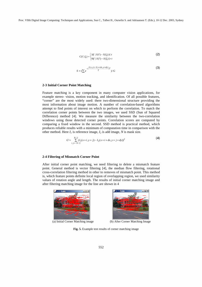
After initial corner point matching, we need filtering to delete a mismatch featurepoint. General method is vector filtering [4], the median flow filtering, rotationalcross-correlation filtering method in other to removes of mismatch point. This methodis, which feature points definite local region of overlapping region, we used similarityvalues of rotation angle and length. The results of initial corner matching image andafter filtering matching image for the line are shown in 4

(a) Initial Corner Matching image (b) After Corner Matching Image

Fig. 5. Example test results of corner matching image

552

Proc. VIIth Digital Image Computing: Techniques and Applications, Sun C., Talbot H., Ourselin S. and Adriaansen T. (Eds.), 10-12 Dec. 2003, Sydney

2-5 Parameter Calculations

Using homogeneous coordinates, 2D planar projective transformation plus affinetransformation method employs the following equations:

+

+

=

z

y

x

T

T

T

Z

Y

X

rrr

rrr

rrr

T

Z

Y

X

R

Z

Y

X

333231

232221

131211

'

'

' (5)

(x, y)=image coordinates, (X,Y,Z)=world coordinates

Geometric correspondence is achieved by determining the mapping function thatgoverns the relationship of all points among a pair of images. There are severalcommon mapping function models in image registration. The general form for themapping function induced by the deformation is [x, y]=[X(u, v), Y(u, v)] where [u, v]and [x, y] denote corresponding pixels in I1 and I2, respectively, and X and Y, arearbitrary mapping function that uniquely specify the spatial transformation. Inregistering I1 and I2, we shall be interested in recovering the inverse mapping functionU and V that transform I2 back into I1 [u, v]=[U(x, y), V(x, y)] In this section, weextend the results of affine registration and Biquadratic using a Taylor series. Theyinclude (1) 3-parameter rigid transformation (translation), (2) 6-parameter affinetransformation (translation, scale, shear) using first-order Taylor series, (3) 12-parameter Biquadratic transformation (translation, rotation, full motion) using second-order Taylor series. We leverage the robust affine registration algorithm to handle themore perspective registration problem. A local affine approximation is suggested byexpanding the perspective transformation function about a point using a first – orderTaylor series. In general, Taylor series equation:

∑∞

=−+

−+−+=

00

0)(

20

0000

)(!

)(

)(2

)(''))((')()(

n

nn

xxn

xf

xxxf

xxxfxfxf L(6)

The approximation holds in a small neighborhood about point (x0, y0). As a result,affine transformation equations: (7)

FEyDxv

CByAxu

++=++= (7)

The affine transformation with first polynomial, it is possibility of the image mosaiccreate according to translation motion. But in the case of rotation, pan and tilt motion,it is difficult to expect good results. It is possible that all movements of camera, (i.e.pan, tilt, rotation, translation, scale, shear), in order to mosaic image creation. Thetraditional method uses perspective transformation using 8-parameters. A weak pointof the method, the calculation process being complicated and the error scope is big. Inorder to overcome the method’s defects, this paper uses second – order Taylor seriespossible full motion mosaic image create. The method is Biquadratic using 12-parameter. The equation (8,9) is Biquadratic (second polynomial) using second-orderTaylor series.

553

Proc. VIIth Digital Image Computing: Techniques and Applications, Sun C., Talbot H., Ourselin S. and Adriaansen T. (Eds.), 10-12 Dec. 2003, Sydney

FxyEyDxCByAx

yyxxy

U

x

Uyy

y

yxUxx

x

yxU

yyy

yxUxx

x

yxUyxU

yxUu

+++++=

−−∂∂

∂∂+−

∂∂

+−∂

∂+

−∂

∂+−∂

∂+=

=

22

00020,0

2

020,0

2

000

000

00

))(()()(

)()(

)(),(

)(),(

),(

),( (8)

LxyKyJxIHyGx

yyxxy

V

x

Vyy

y

yxVxx

x

yxV

yyy

yxVxx

x

yxVyxV

yxVv

+++++=

−−∂∂

∂∂+−

∂∂

+−∂

∂+

−∂

∂+−∂

∂+=

=

22

00020,0

2

020,0

2

000

000

00

))(()()(

)()(

)(),(

)(),(

),(

),( (9)

Compared with Affine transformation and Biquadratic, Affine transformation ispossible slow-moving camera movement and translation motion be unchangedviewpoint of users. But optical rolling motion of the camera to free motion it cannotobtain good result. Biquadratic algorithm can obtain good result free motions ofcamera, rotation, rolling, zoom in and zoom out. For example affine transformation,given the four corners of a tile in observed image I2 and their correspondences onreference image I1, we may solve for the best affine fit by using the least squaresapproach. We may relate these correspondence in the form U=WA. Eq (10):

=

F

E

D

C

B

A

yx

yx

yx

yx

v

v

u

u

1000

1000

0001

0001

44

11

44

11

4

1

4

1

MMMMMM

MMMMMM

M

M(10)

The pseudoinverse solution A=(WTW)-1WTU is computed to solve for the six affinecoefficients. After finding the transformation function for each successive image pair,we compute the transformation function of each image relative to the base imagebased on the associative of the matrix multiplication. Then, we can combine all of theimage frames into one big image.

2-6 Interpolation

Interpolation process can be classified into four methods (i.e. Nearest Neighborinterpolation, Bilinear interpolation, Cubic Convolution, B – Spline interpolation). Inthis approach, we used bilinear interpolation. A critical portion of warping images isinterpolation for the resulting pixel values. Without a decent facility for interpolation,precise movement in the error minimization technique would not be possible. Theprocess of bilinear interpolation requires four neighboring values to the coordinate atwhich we need to interpolation. The interpolation is performed in a separable manneras illustrated by the diagram below. First, the interpolation occurs in the X direction,followed by an interpolation in the Y direction.

554

Proc. VIIth Digital Image Computing: Techniques and Applications, Sun C., Talbot H., Ourselin S. and Adriaansen T. (Eds.), 10-12 Dec. 2003, Sydney

3. Experimental Results

To evaluate the performance of our proposed algorithm, we implemented in visualC++ language. The test images we used were obtained in the outside scene and insideusing hand held camera for minimum time interval. Since only 2D motion parameterswere estimated, the test images were constrained to or close to planar imagesequences. Each color image has 640×480, 320×240 pixels, and image format hasJEPG, BMP. In general, feature based correlation is sensitive to rotation motion. Inorder to feature matching, we need feature matching point more than 40 point. Usingour proposed approach, part of matching took 60% of total processing time.Processing time results of two images for different processing are shown in Table.1.Total processing time is different each image, (i.e. image size, natural scene, insidescene, difficult scene…). Fig. 5. Shows the result image using the affinetransformation (6-parameter) and Fig. 6. Shows the result image using Biquadratic(12-paramater).. In Fig. 7, shows the results of test image. The display is shown inFig. 8

Fig. 6. The result image using affine transformation. Fig. 7. result image using Biquadratic

(Unit: seconds)

Image size Feature extraction Initial matching Filtering Total time

320�240 1 1.30 1 4

640�480 2 7 4 16

Table 1. The result of processing time

4. Conclusions

We have presented a distributed image mosaic system that can quickly, hand heldcamera full motion and automatically align a sequence of images to create a largerimage. A further direction of this research will be effective algorithm development forshorten the corner matching process time and blending processing for naturalboundary region.

555

Proc. VIIth Digital Image Computing: Techniques and Applications, Sun C., Talbot H., Ourselin S. and Adriaansen T. (Eds.), 10-12 Dec. 2003, Sydney

(a) reference image (b) add image

(c) result image of using affine transformation (d) result image of using Biquadratic

Fig. 8. Results of test images Fig. 9. The interface of image mosaic create system

Reference

1 Richard Szeliski, “ Image Mosaicing for tele Reality applications”, Cambridge Research LabTechnical Report, May 1984

2 Richard Szeliski,HeungYeung Shum”Creating Full View Panoramic image Mosaic andEnvironment maps”, SIGRAPH 87, pp 251~258

3 S.M Smith and J,M Brady, ”Susan a new Approach to low level image processing”,Technical Report TR95SMSIc, 1995

4 P.Smithm, D Sinclaif, R. Cipolla and K. Wood, “Effective Corner matching”, Britishmachine vision conference, Vol 2 p 545~556, September 1998

5 Richard Szeliski, "Video mosaics for virtual Environments", IEEE Computer Graphics andApplication, 1966, pp 22�30.

6 Naoki CHIBA, Hiroshi KANO, Michihiko MINOH and Masashi YASUDA “Feature –basedimage mosaicng”, IEICE, Japan D-II Vol, J82 No 10 pp 1589~1999 1999.10

556

Proc. VIIth Digital Image Computing: Techniques and Applications, Sun C., Talbot H., Ourselin S. and Adriaansen T. (Eds.), 10-12 Dec. 2003, Sydney