Embed Size (px)
Citation preview

Automatic High-Performance Kernel Generation for DL Accelerators : Specialization to Generalization*
Prasanth Chatarasi Research Staff Member @ AI Hardware Group,
IBM T.J. Watson Research Center,YorkTown Heights, NY, USA
https://www.research.ibm.com/artificial-intelligence/hardware/[email protected]
Google Brain, May 26th, 2021
*Work done during PhD studies in Habanero Research Group at Georgia Institute of Technology
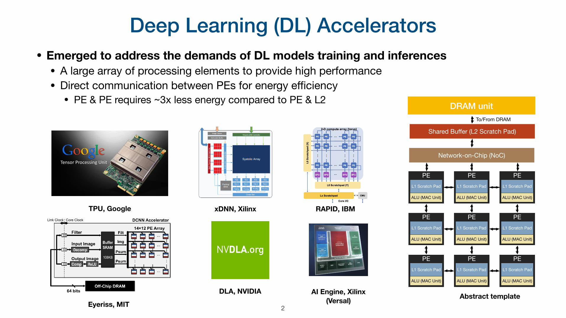
Deep Learning (DL) Accelerators• Emerged to address the demands of DL models training and inferences • A large array of processing elements to provide high performance• Direct communication between PEs for energy efficiency • PE & PE requires ~3x less energy compared to PE & L2
2
PE
Shared Buffer (L2 Scratch Pad)
Network-on-Chip (NoC)
L1 Scratch Pad
ALU (MAC Unit)
To/From DRAM
PEL1 Scratch Pad
ALU (MAC Unit)
PEL1 Scratch Pad
ALU (MAC Unit)
PEL1 Scratch Pad
ALU (MAC Unit)
PEL1 Scratch Pad
ALU (MAC Unit)
PEL1 Scratch Pad
ALU (MAC Unit)
PEL1 Scratch Pad
ALU (MAC Unit)
PEL1 Scratch Pad
ALU (MAC Unit)
PEL1 Scratch Pad
ALU (MAC Unit)
DRAM unit
Abstract templateEyeriss, MIT
TPU, Google xDNN, Xilinx RAPID, IBM
DLA, NVIDIA AI Engine, Xilinx (Versal)

Design Architecture of Deep Learning (DL) Compilers
3
Li et. al., “The Deep Learning Compiler: A Comprehensive Survey”, ArXived 2020
Key steps in the flow: • Graph compiler performing
graph-level optimizations • e.g., Node/Layer fusion
• Kernel compiler performing kernel-level optimizations• e.g., loop scheduling

Kernel Compilers of DL Compiler stack
4
Li et. al., “The Deep Learning Compiler: A Comprehensive Survey”, ArXived 2020
Three major approaches for kernel compilers: • Stitch manually-written
kernel libraries for each node of the optimized graph
• Automatically generate entire kernels corresponding to each node of the graph
• Hybrid approach combining some parts with manually-written kernels and other parts with automatic generation
Manually-written vs Automatically-generated
5
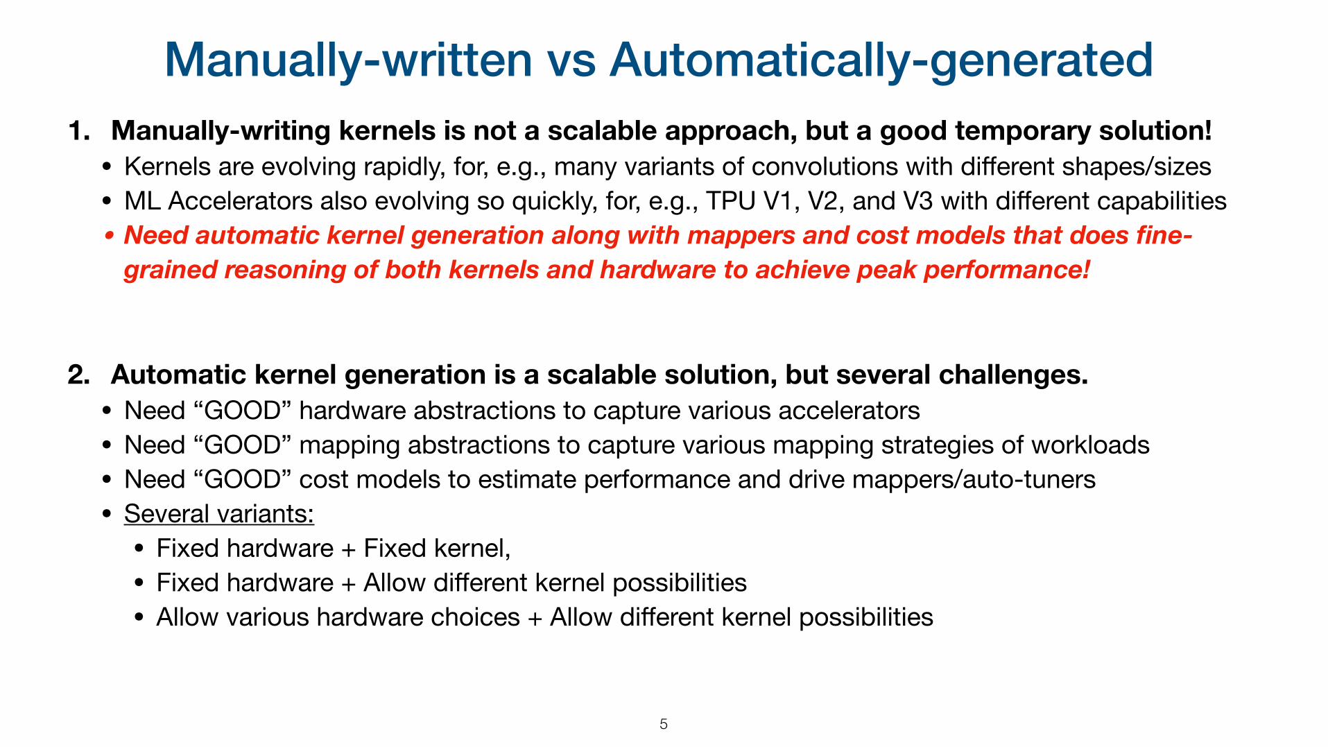
1. Manually-writing kernels is not a scalable approach, but a good temporary solution! • Kernels are evolving rapidly, for, e.g., many variants of convolutions with different shapes/sizes• ML Accelerators also evolving so quickly, for, e.g., TPU V1, V2, and V3 with different capabilities• Need automatic kernel generation along with mappers and cost models that does fine-
grained reasoning of both kernels and hardware to achieve peak performance!
2. Automatic kernel generation is a scalable solution, but several challenges. • Need “GOOD” hardware abstractions to capture various accelerators• Need “GOOD” mapping abstractions to capture various mapping strategies of workloads• Need “GOOD” cost models to estimate performance and drive mappers/auto-tuners• Several variants: • Fixed hardware + Fixed kernel, • Fixed hardware + Allow different kernel possibilities• Allow various hardware choices + Allow different kernel possibilities

Overview of today’s talk
6
1. Introduction & Background
2. Vyasa: A High-performance Vectorizing Compiler for Tensor Operations onto Xilinx AI Engine (2D SIMD unit)• Fixed hardware + Allow different kernel possibilities
3. PolyEDDO: A Polyhedral-based Compiler for Explicit De-coupled Data Orchestration (EDDO) architectures • Allow various hardware choices + Allow different kernel possibilities
4. Conclusions
Overview of today’s talk
7
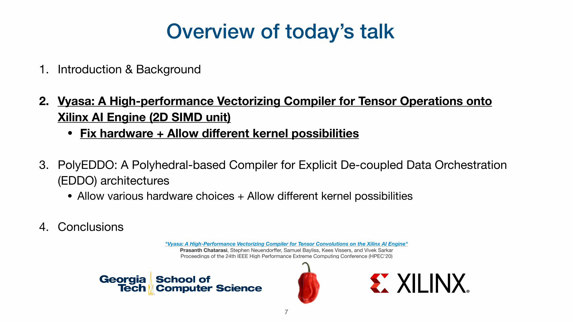
1. Introduction & Background
2. Vyasa: A High-performance Vectorizing Compiler for Tensor Operations onto Xilinx AI Engine (2D SIMD unit) • Fix hardware + Allow different kernel possibilities
3. PolyEDDO: A Polyhedral-based Compiler for Explicit De-coupled Data Orchestration (EDDO) architectures • Allow various hardware choices + Allow different kernel possibilities
4. Conclusions"Vyasa: A High-Performance Vectorizing Compiler for Tensor Convolutions on the Xilinx AI Engine"
Prasanth Chatarasi, Stephen Neuendorffer, Samuel Bayliss, Kees Vissers, and Vivek Sarkar Proceedings of the 24th IEEE High Performance Extreme Computing Conference (HPEC'20)

Xilinx Versal AI Engine• A High Performance & Power Efficient VLIW SIMD Core • Part of Xilinx Versal Advanced Compute Acceleration Platform• Scalar Engines (CPUs), Adaptable Engines (Programmable logic), Intelligent Engines (AI Engines)
8 Xilinx Public Domain

Key architectural features of AI Engine
9
….
….
….
….
L0
L1
L15
C0 C1
Shuffle (interconnect) network
Vector register file (256B)
Local memory (128KB)
….
….
….
C7
Fixed Point SIMD Unit
Abstract view of AI Engine 1) 2D SIMD datapath for fixed point
2) Shuffle Interconnection network• Between SIMD and vector register file• Supports arbitrary selection of elements from
a vector register• Some constraints for 16-/8-bit types
• Selection parameters are provided via vector intrinsics
• Reduction within a row/lane• #Columns depend on operand precision• 32-bit types: 8 rows x 1 col• 16-bit types: 8 rows x 4 col (or)
16 rows x 2 col• 8-bit types: 16 rows x 8 col
Problem Statement & Challenges
10
Problem statement: How to implement high-performance primitives for tensor convolutions on AI Engine?
• Current practice: Programmers manually use vector intrinsics to program 2D SIMD unit and also explicitly specify shuffle network parameters for data selection
Our approach: Vyasa, a domain-specific compiler to generate high performance primitives for tensor convolutions from a high-level specification
• Challenges: Error prone, written code may not be portable to a different schedule or data-layouts, daunting to explore all choices to find best implementation, tensor convolutions vary in sizes and types
Vyasa means “compiler” in the Sanskrit language, and also refers to the sage who first compiled the Mahabharata.
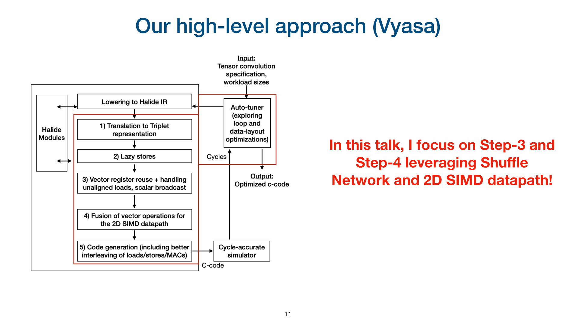
Our high-level approach (Vyasa)
11
In this talk, I focus on Step-3 and Step-4 leveraging Shuffle
Network and 2D SIMD datapath!

⊗
0
0 1815
W
I
Running Example — CONV1D
12
for(x=0; x < 16; x++) for(w=0; w < 4; w++) O[x] += I[x+w]*W[w];
A sample schedule: Unroll w-loop and Vectorize x-loop (VLEN: 16)
O(0:15) += W(0) * I(0:15) O(0:15) += W(1) * I(1:16) O(0:15) += W(2) * I(2:17) O(0:15) += W(3) * I(3:18)
1 2 3
Input Weight Output=⊗16419

Challenges
13
V1 = VLOAD(I, 0:15); V2 = BROADCAST(W, 0); V3 = VMAC(V1, V2);
V4 = VLOAD(I, 1:16); V5 = BROADCAST(W, 1); V3 = VMAC(V3, V4, V5);
V6 = VLOAD(I, 2:17); V7 = BROADCAST(W, 2); V3 = VMAC(V3, V6, V7);
V8 = VLOAD(I, 3:18); V9 = BROADCAST(W, 3); V3 = VMAC(V3, V8, V9); VSTORE(O, 0:15, V3);
No support for unaligned loads
O(0:15) += W(0) * I(0:15) O(0:15) += W(1) * I(1:16) O(0:15) += W(2) * I(2:17) O(0:15) += W(3) * I(3:18)
No support for broadcast operations
V6 and V8 have 15 elements in common. How to reuse them without loading again?
How to exploit multiple columns of 2D vector substrate?
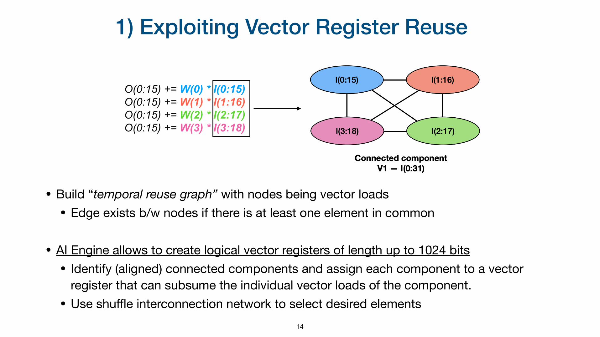
1) Exploiting Vector Register Reuse
14
• Build “temporal reuse graph” with nodes being vector loads• Edge exists b/w nodes if there is at least one element in common
• AI Engine allows to create logical vector registers of length up to 1024 bits • Identify (aligned) connected components and assign each component to a vector
register that can subsume the individual vector loads of the component.• Use shuffle interconnection network to select desired elements
O(0:15) += W(0) * I(0:15) O(0:15) += W(1) * I(1:16) O(0:15) += W(2) * I(2:17) O(0:15) += W(3) * I(3:18)

2) Exploiting Spatial Locality
15
• Build “spatial locality graph” with nodes being scalar loads• Edge exists b/w nodes if they can be part of an aligned vector load
• Identify connected components • AI Engine allows to create logical vector registers of length up to 1024 bits • Assign each connected component (aligned) to a logical vector register• Use shuffle interconnection network to select desired elements
O(0:15) += W(0) * I(0:15) O(0:15) += W(1) * I(1:16) O(0:15) += W(2) * I(2:17) O(0:15) += W(3) * I(3:18)

3) Grouping 1D Vector Operations O(0:15) += W(0) * I(0:15) O(0:15) += W(1) * I(1:16) O(0:15) += W(2) * I(2:17) O(0:15) += W(3) * I(3:18)
All the 4 operations are performed with a single load of V1 and V2 (maximum reuse)

Our high-level approach (Vyasa)
17
Auto-tuner explores the space of schedules related to
loop and data-layouts.
Loop transformations: 1. Choice of vectorization loop2. Loop reordering3. Loop unroll and jam
Data-layout choices: 1. Data permutation2. Data tiling (blocking)
We assume that workload memory footprint fits into a AI Engine local scratchpad memory (128KB)
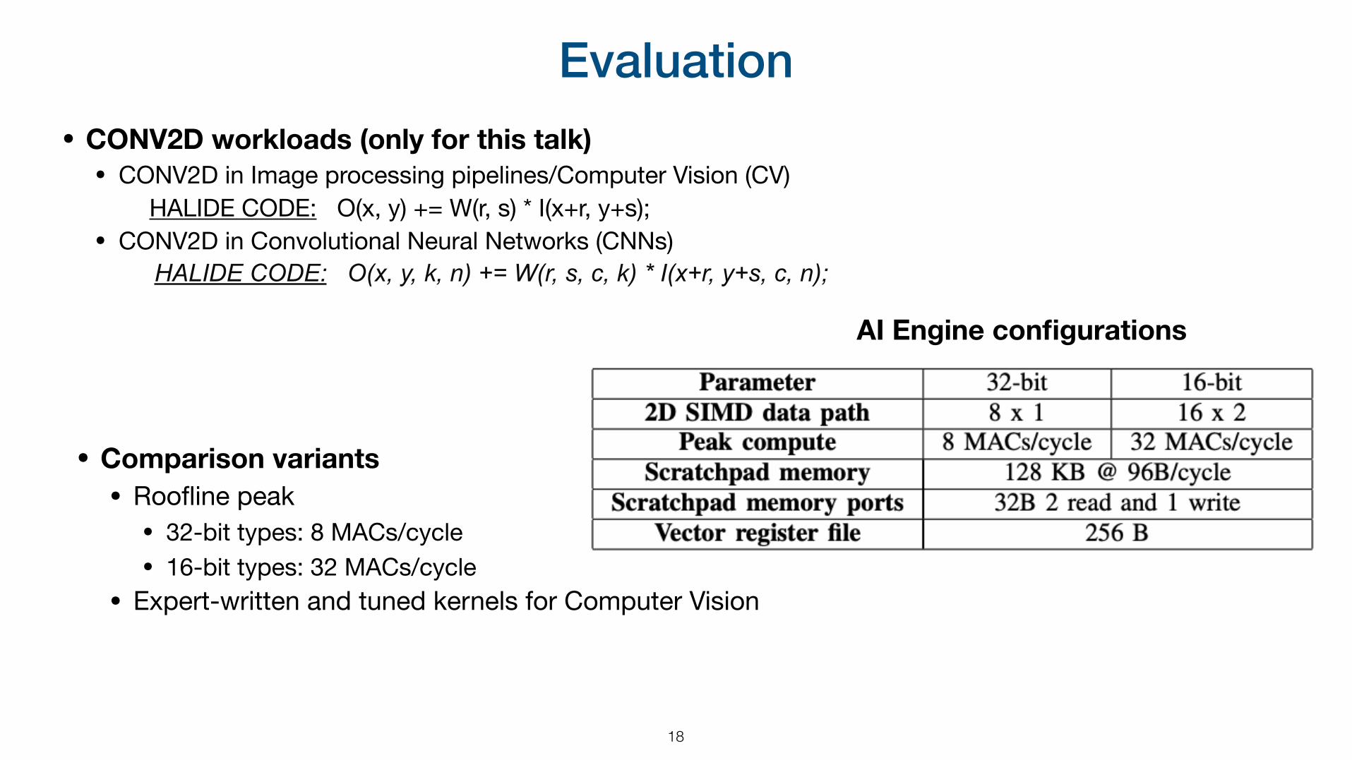
Evaluation
18
• Comparison variants • Roofline peak • 32-bit types: 8 MACs/cycle• 16-bit types: 32 MACs/cycle
• Expert-written and tuned kernels for Computer Vision
AI Engine configurations
• CONV2D workloads (only for this talk) • CONV2D in Image processing pipelines/Computer Vision (CV)
HALIDE CODE: O(x, y) += W(r, s) * I(x+r, y+s);• CONV2D in Convolutional Neural Networks (CNNs)
HALIDE CODE: O(x, y, k, n) += W(r, s, c, k) * I(x+r, y+s, c, n);

Evaluation: CONV2D’s in CV (256x16)
19
• Expert-written codes are available only for 3x3 and 5x5 filters • Available as part of the Xilinx’s AI Engine compiler infrastructure
• Auto-tuner was able to find better schedules • Especially non-trivial unroll and jam factors
MAC
s/C
ycle
0
10
20
30
40
3x3 (32-bit) 5x5 (32-bit) 3x3 (16-bit) 5x5 (16-bit) Geo. Mean (32-bit) Geo. Mean (16-bit)
32.00
8.00
32.0032.00
8.008.00
22.69
7.87
23.6521.76
7.917.83
20.45
7.20
23.30
17.95
7.556.85
Expert-Written Our approach with auto-tuner AI Engine Peak
HALIDE CODE: O(x, y) += W(r, s) * I(x+r, y+s);

Evaluation: CONV2D’s in CV (256x16) with various Filters
20
• Even-sized filters (except 2x2), our approach achieved close to peak • 87% for 16-bit and 95% for 32-bit
• Odd-sized filters, our approach padded each row with an additional column • For 16-bit type, number of reductions should be multiple of two (2 columns)
MAC
s/C
ycle
0
6
13
19
25
31
38
44
50
2x2 3x3 4x4 5x5 6x6 7x7 8x8 9x9 10x10 11x11 Geo. Mean
25.9227.0828.4526.49
29.3326.2027.54
23.65
28.53
21.7621.59
7.677.267.227.637.607.917.887.917.857.837.62
Our approach with auto-tuner for 32-bit types (AI Engine Peak : 8 MACs/cycles) Our approach with auto-tuner for 16-bit types (AI Engine Peak : 32 MACs/cycles)

Evaluation: CONV2D’s in CNN’s (128x2x16)
21
• REG-CONV2D (3x3, 5x5, 7x7) • Vectorization along Output width and Reduction along Filter channels
• PW-CONV2D (1x1), SS-CONV2D (1x3, 3x1), FC-CONV2D (1x1) • Vectorization along Output channels and Reduction along Filter channels
• DS-CONV2D (3x3) — Padded each row • Vectorization along Output width and Reduction along Filter width
MAC
s/C
ycle
0
5
10
15
20
25
30
35
40
REG-3x3 REG-5x5 REG-7x7 PW-1x1 SS-1x3 SS-3x1 DS-3x3 FC-1x1 Geo. Mean
22.53
15.77
19.6922.3422.47
24.9428.37
26.60
22.62
7.677.947.467.887.897.757.837.457.19
Our approach with auto-tuner for 32-bit types (AI Engine Peak: 8 MACs/cycles) Our approach with auto-tuner for 16-bit types (AI Engine Peak: 32 MACs/cycles)
HALIDE CODE for REG CONV2D: O(x, y, k, n) += W(r, s, c, k) * I(x+r, y+s, c, n);

Non-trivial data-layout choices
22
• 16-bit REG-CONV2D (3x3) • Vectorization along Output width and Reduction along Filter channels• For the fused vector operation (W1xI1 + W2 x I2)• Data for (I1, I2) should be in a single vector register for the operation• I1(0) and I2(0) should be adjacent for shuffle network constraints
• (C/2)Y’X’(2) refers to first laying out an input block of two channels followed by width, height, and remaining channels.

Summary and Questions
23
• Summary • Manually writing vector code for high-performant tensor convolutions achieving
peak performance is extremely challenging!• Automatic kernel generation can be the key! • Proposed a convolution-specific IR for easier analysis and transformations• Our approach (Vyasa) can work for any convolution variant regardless of its
variations and shapes/sizes.• Achieved close to the peak performance for a variety of tensor convolutions
• Questions • How about beyond tensor-style operations?• E.g., fused convolutions (depth-wise + point-wise), non-rectilinear iteration spaces
(Symmetric GEMM)• How about beyond the AI Engine? • E.g., other accelerators like IBM Rapid, MIT Eyeriss, NVDLA…

Overview of today’s talk
24
1. Introduction & Background
2. Vyasa: A High-performance Vectorizing Compiler for Tensor Operations onto Xilinx AI Engine (2D SIMD unit)• Fixed hardware + Allow different kernel possibilities
3. PolyEDDO: A Polyhedral-based Compiler for Explicit De-coupled Data Orchestration (EDDO) architectures • Allow various hardware choices + Allow different kernel possibilities
4. Conclusions"Hardware Abstractions for targeting EDDO Architectures with the Polyhedral Model"
Angshuman Parashar, Prasanth Chatarasi, and Po-An Tsai, 11th International Workshop on Polyhedral Compilation Techniques (IMPACT'21)

ICDO vs EDDO Architectures
EDDO architectures attempt to minimize data movement costs
Buffer
× × × ×
L2
L1
Buffer
DRAML3
RegFile RegFile RegFile RegFile
× × × ×
RegFile RegFile RegFile RegFile
L2 CacheL2 L2 Cache
DRAML3
× × × ×
L1
Datapaths
L1$ L1$ L1$
× × × ×
L1$ L1$ L1$ L1$L1$
Implicit Coupled Data Orchestration (ICDO) e.g., CPUs, GPUs
Explicit Decoupled Data Orchestration (EDDO) e.g., IBM Rapid AI, NVIDIA Simba, NVDLA, Eyeriss, etc.
Addr Gen
Addr Gen
Distributor
Distributor CollectorAddr Gen
Datapaths

EDDO Architectures
26
Benefits • Dedicated (and often statically
programmed) state machines more efficient than general cores • Perfect “prefetching” • Buffet storage idiom provides
fine-grain synchronization and efficient storage, or scratchpads + Send/Recv synchronization • Hardware mechanisms for reuse
Buffer
× × × ×
L2
L1
Datapaths
Buffer
DRAML3
RegFile RegFile RegFile RegFile
× × × ×
RegFile RegFile RegFile RegFile
Addr Gen
Addr Gen
Distributor
Distributor CollectorAddr Gen
Pellauer et. al., “Buffets: An Efficient and Composable Storage Idiom for Explicit Decoupled Data Orchestration”, ASPLOS 2019
Explicit Decoupled Data Orchestration (EDDO) e.g., IBM Rapid AI, NVIDIA Simba, NVDLA, Eyeriss, etc.

EDDO Architectures
27
Challenges 1. No single binary: Collection of distinct
binaries that program distributed state machines working together to execute algorithm • E.g., CNN layer on EDDO arch ! ~250 distinct state
machines.
2. Reuse optimization is critical for efficiency • E.g., CNN layer on EDDO arch ! 480,000 mappings, 11x
spread in energy efficiency, 1 optimal mapping • Need an optimizer or mapper
3. Variety of EDDO architectures, constantly evolving • Need an abstraction that Mapper and Code Generator will
target
Buffer
× × × ×
L2
L1
Datapaths
Buffer
DRAML3
RegFile RegFile RegFile RegFile
× × × ×
RegFile RegFile RegFile RegFile
Addr Gen
Addr Gen
Distributor
Distributor CollectorAddr Gen
Mapper (optimizer)
Code Generator
MappingWorkload Binaries
Explicit Decoupled Data Orchestration (EDDO) e.g., IBM Rapid AI, NVIDIA Simba, NVDLA, Eyeriss, etc.

28
Overall Compilation Flow
Mapper * (optimizer) PolyEDDO Code Generator
Mapping
Workload Configuration BinariesArch-specific configuration generator
Arch-independent decoupled programs
Analytical microarchitecture and
energy model †
Perf, Energy, AreaData-movement activity counts
EDDO Architecture described using Hardware
Space-Time (HST)
*† Parashar et. al., “Timeloop: Timeloop: A Systematic Approach to DNN Accelerator Evaluation”, ISPASS 2019 † Wu et. al., “Accelergy: An Architecture-Level Energy Estimation Methodology for Accelerator Designs”, ICCAD 2019

29
Example1 — Symbolic Hardware Space-Time (SHST)
t1
s1
L1
L2
Buffer
× × × ×
L2
L1
MACCs
𝑆𝑝𝑎𝑐𝑒𝑇𝑖𝑚𝑒2 [𝑠2, 𝑡2] →𝑆𝑝𝑎𝑐𝑒𝑇𝑖𝑚𝑒1 [𝑠1, 𝑡1] :
𝑠2 = 0 & 𝑡2 = 0 & 0 ≤ 𝑠1 < 4 & 0 ≤ 𝑡1 < 3
Single L2, 4 L1s, 3 time-steps • In each step, the L2 delivers a tile of data to
each L1 • Across all these L1 time steps, the resident tile
in L2 does not change. In effect, time is stagnant for L2

30
Example2 — Symbolic Hardware Space-Time (SHST)
Buffer
× × × ×
L2
L1
MACCs
Buffer
× × × ×MACCs
DRAML3
𝑆𝑝𝑎𝑐𝑒𝑇𝑖𝑚𝑒3 [𝑠3, 𝑡3] → [𝑆𝑝𝑎𝑐𝑒𝑇𝑖𝑚𝑒2 [𝑠2, 𝑡2] →𝑆𝑝𝑎𝑐𝑒𝑇𝑖𝑚𝑒1 [𝑠1, 𝑡1]] :
𝑠3 = 0 𝑡3 = 0 0 ≤ 𝑠2 < 2 0 ≤ 𝑡2 < 2 0 ≤ 𝑠1 < 4 0 ≤ 𝑡1 < 3
t1 t1
t1
s1
L1
L2
s2
t2
L3
s1 s1
𝑆𝑝𝑎𝑐𝑒𝑇𝑖𝑚𝑒3[0,0] → 𝑆𝑝𝑎𝑐𝑒𝑇𝑖𝑚𝑒2[1,1]
𝑆𝑝𝑎𝑐𝑒𝑇𝑖𝑚𝑒3[0,0] → [𝑆𝑝𝑎𝑐𝑒𝑇𝑖𝑚𝑒2[1,0] → 𝑆𝑝𝑎𝑐𝑒𝑇𝑖𝑚𝑒1 [2,1]]

31
Example3 — Partitioned Buffers
PHSTDRAM [𝑠3, 𝑡3]
BufA [𝑠2, 𝑡2]BufB [𝑠2, 𝑡2]BufZ [𝑠2, 𝑡2]
OperandA [2𝑠2 + 𝑠1, 𝑡2, 𝑡1]OperandB [2𝑠2 + 𝑠1, 𝑡2, 𝑡1]
ΘHST(DRAM) = →𝑆𝑝𝑎𝑐𝑒𝑇𝑖𝑚𝑒3 [0, 0]
𝑆𝑝𝑎𝑐𝑒𝑇𝑖𝑚𝑒3 [0, 0] → 𝑆𝑝𝑎𝑐𝑒𝑇𝑖𝑚𝑒2 [𝑠2, 𝑡2] →ΘHST(BufA) =
𝑆𝑝𝑎𝑐𝑒𝑇𝑖𝑚𝑒3 [0, 0] → 𝑆𝑝𝑎𝑐𝑒𝑇𝑖𝑚𝑒2 [𝑠2, 𝑡2] →ΘHST(BufB) =
𝑆𝑝𝑎𝑐𝑒𝑇𝑖𝑚𝑒3 [0, 0] → 𝑆𝑝𝑎𝑐𝑒𝑇𝑖𝑚𝑒2 [𝑠2, 𝑡2] →ΘHST(BufZ) =
𝑆𝑝𝑎𝑐𝑒𝑇𝑖𝑚𝑒3 [0, 0] → [𝑆𝑝𝑎𝑐𝑒𝑇𝑖𝑚𝑒2 [𝑠2, 𝑡2] →𝑆𝑝𝑎𝑐𝑒𝑇𝑖𝑚𝑒1 [𝑠1, 𝑡1]] →ΘHST(OperandA) =
𝑆𝑝𝑎𝑐𝑒𝑇𝑖𝑚𝑒3 [0, 0] → [𝑆𝑝𝑎𝑐𝑒𝑇𝑖𝑚𝑒2 [𝑠2, 𝑡2] →𝑆𝑝𝑎𝑐𝑒𝑇𝑖𝑚𝑒1 [𝑠1, 𝑡1]] →ΘHST(OperandB) =
𝑆𝑝𝑎𝑐𝑒𝑇𝑖𝑚𝑒3 [0, 0] → [𝑆𝑝𝑎𝑐𝑒𝑇𝑖𝑚𝑒2 [𝑠2, 𝑡2] →𝑆𝑝𝑎𝑐𝑒𝑇𝑖𝑚𝑒1 [𝑠1, 𝑡1]] →ΘHST(Result) = Result [2𝑠2 + 𝑠1, 𝑡2, 𝑡1]
𝑆𝑝𝑎𝑐𝑒𝑇𝑖𝑚𝑒3 [𝑠3, 𝑡3] → [𝑆𝑝𝑎𝑐𝑒𝑇𝑖𝑚𝑒2 [𝑠2, 𝑡2] →𝑆𝑝𝑎𝑐𝑒𝑇𝑖𝑚𝑒1 [𝑠1, 𝑡1]]
HST
SHST
BufB
DRAM
BufA BufZ
× × × ×
BufBBufA BufZ
× × × ×
BufB
DRAM
BufA BufZ
× × × ×
BufBBufA BufZ
× × × ×
BufBL2
L1
MACCs
DRAML3
BufA BufZ
× × × ×OperandA
OperandB
Result
BufBBufA BufZ
× × × ×t1 t1
t1
s1
L1
L2
s2
t2
L3
s1 s1Workload mappings target SHST
t1
t2
t3

32
Example4 — Eyeriss-like accelerator
× × × ×
× × × ×
× × × ×
DRAM
DiagBuffer
DiagBroadcaster
ColSpatialReducer
ColBuffer
Row
Broa
dcas
terRowBuffer
OperandA
OperandB
Result
L1
L2
L3
L4
SHST: 𝑆𝑝𝑎𝑐𝑒𝑇𝑖𝑚𝑒4 [𝑠4, 𝑡4] → 𝑆𝑝𝑎𝑐𝑒𝑇𝑖𝑚𝑒3 [𝑠3, 𝑡3] → [𝑆𝑝𝑎𝑐𝑒𝑇𝑖𝑚𝑒2 [𝑠2, 𝑡2] →𝑆𝑝𝑎𝑐𝑒𝑇𝑖𝑚𝑒1 [𝑠1, 𝑡1]]
Workload mappings target SHST
See paper for full HST
Observe how different the architecture is from CPUs and GPUs

33
PolyEDDO Code Generator
T-relation generation
Decoupling
Reuse Analysis
Schedule creation
AST generation
WorkloadArchitecture HST
Mapping
Tiling (T)-relations
Delta (∆)-relations
Data Transfer (X)-relations
∆ schedules
Decoupled ASTs

34
Mapping workloads (Tensor operations)M
N
Tile
Tile
Project
Project
Project
Workload Iteration
Space
t1 t1
t1
s1
L1
L2
s2
t2
L3
SHST
s1 s1

35
Mapping workloads (The Tiling-relation, T-relation)
𝑆𝑝𝑎𝑐𝑒𝑇𝑖𝑚𝑒3[0,0] → 𝑆𝑝𝑎𝑐𝑒𝑇𝑖𝑚𝑒2[1,1]
𝑆𝑝𝑎𝑐𝑒𝑇𝑖𝑚𝑒3[0,0] → [𝑆𝑝𝑎𝑐𝑒𝑇𝑖𝑚𝑒2[1,0] → 𝑆𝑝𝑎𝑐𝑒𝑇𝑖𝑚𝑒1 [2,1]]
t1 t1
t1
s1
L1
L2
s2
t2
L3SHST
s1 s1
→ MatrixA[m,k] : … MatrixB[k,n] : … MatrixZ[m,n] : …
→ MatrixA[m,k] : … MatrixB[k,n] : … MatrixZ[m,n] : …
Set of Tensor Coords
Set of Tensor Coords
T-relation: Projection from SHST coordinate to a set of tensor coordinates • Tells you what tiles of data must be present at
that point in space-time to honor the mapping. • Does not tell you how the data got there.

36
Decoupling — Breaking the hierarchy
BufBL2
L1
MACCs
DRAML3
BufA BufZ
× × × ×OperandA
OperandBResult
BufB
BufA BufZ
× × × ×
BufBL2
DRAML3
BufA BufZ BufBBufA BufZ
BufBL2
L1
BufA BufZ BufBBufA BufZ
L1
MACCs
× × × × × × × ×
M
N
t1 t1
t1
s1
L1
L2
s2
t2
L3SHST
s1 s1
T-relations
PHST
HST Decouple
PHSTTensor coords
[DRAM[s3, t3] -> BufA[s2, t2]] -> W[k, r] : …
[BufA[s2, t2] -> OperandA[s1, t1]] -> W[k, r] : …
[MACC[s1, t1]] -> MulAcc[k, p, r] : …
Data transfer relations (X-relations)

37
REUSE ANALYSIS
t
ss
t
t
s
L1
L2
Local Temporal Reuse

38
REUSE ANALYSIS
t
ss
t
t
s
L1
L2
Fill from Peer
39
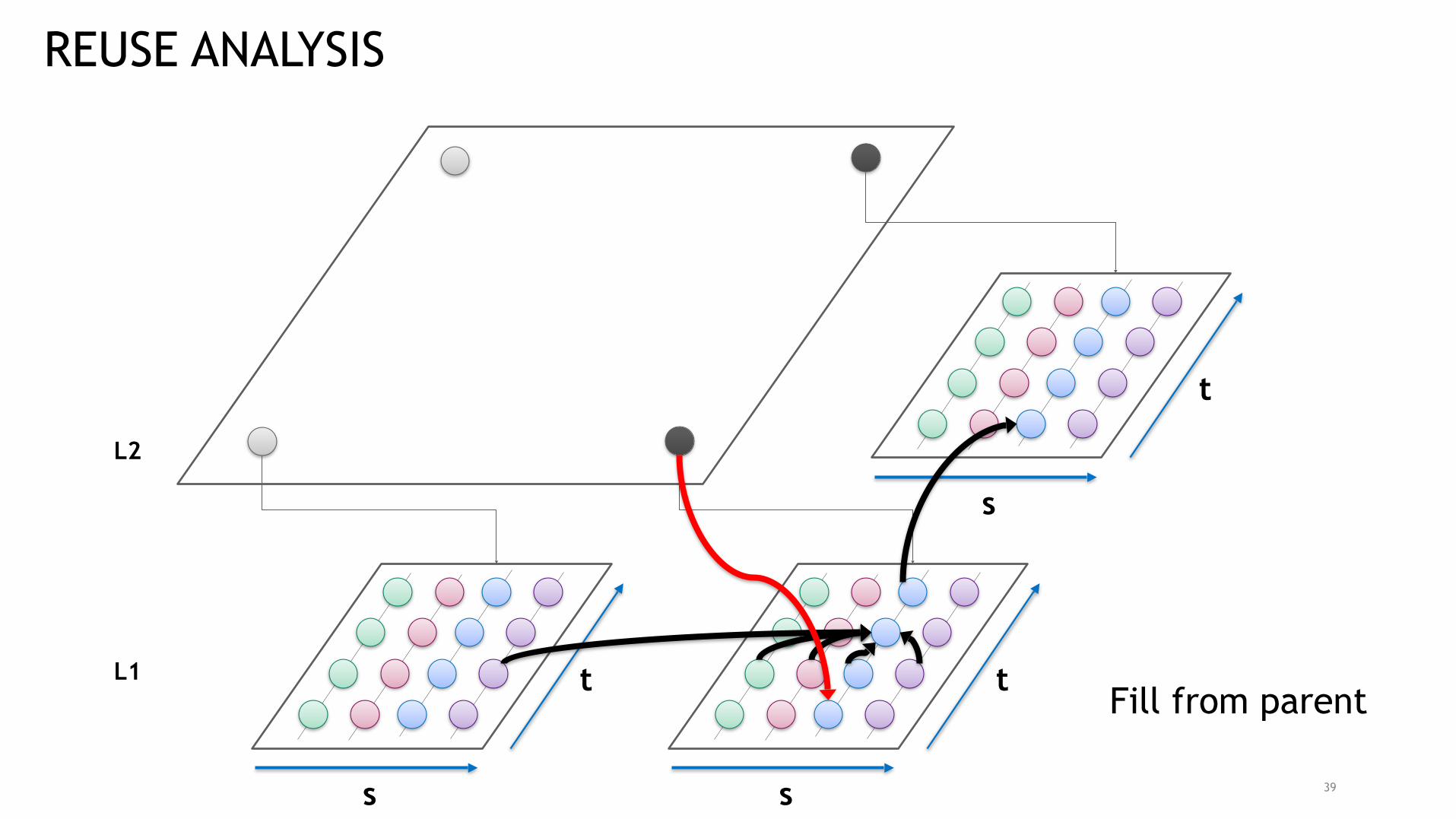
REUSE ANALYSIS
t
ss
t
t
s
L1
L2
Fill from parent

40
REUSE ANALYSIS
t
ss
t
t
s
L1
L2
Parent Multicast/ Spatial Reduction

41
OPTIMIZATION PROBLEM (FOR A SINGLE MAPPING!)
From Peer A From Peer B
From Parent
Local Reuse Options:
1. Enumerate all possibilities and find optimum solution
2. Use a heuristic
3. Expose choices to mapping (and thereby the mapspace)

42
POLYEDDO
T-relation generation
Decoupling
Reuse Analysis
Schedule creation
AST generation
WorkloadArchitecture HST
Mapping
Tiling (T)-relations
Delta (∆)-relations
Data Transfer (X)-relations
∆ schedules
Decoupled ASTs
Described in paper

43
EXAMPLE OUTPUT
• Present capability: build generated code against an EDDO emulator (automatically configured from the PHST)

Summary and Questions?
44
• Summary • HST (Hardware Space-Time) – an abstraction for EDDO architectures represented
using the Polyhedral Model• PolyEDDO (WIP) – an analysis and code-generation flow based on HST
• Research questions • How do we think about mapping imperfectly-nested loops to generic EDDO
architectures?• How do we capture sparsity extensions of the accelerators?

Acknowledgments
45
• Ph.D. Advisors: • Vivek Sarkar (advisor), and Jun Shirako (co-advisor)
• Collaborators • Albert Cohen, Martin Kong, Tushar Krishna, Hyoukjun Kwon, John Mellor-
Crummey, Karthik Murthy, Stephen Neuendorffer, Angshuman Parashar, Micheal Pellauer, Kees Vissers, and others
• Other mentors • Kesav Nori, Uday Bondhugula, Milind Chabbi, Shams Imam, Deepak
Majeti, Rishi Surendran, and others
• IBM Research, Habanero & Synergy Research Group Members

Backup
46

Why do we need accelerators?
47
1) DNN models have tight constraints on latency, throughput, and energy consumption, esp. on edge devices
2) DNN models have trillions of computationsNeed high throughput — Makes CPUs inefficient
3) DNN models involve heavy data movementNeed to reduce energy — Makes GPUs inefficient
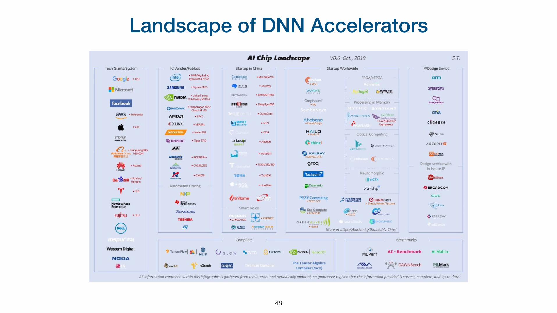
Landscape of DNN Accelerators
48


![Towards Automatic Inference of Kernel Object Semantics ...cloudcomputing.ieee.org/.../publications/articles/... · ory forensics (e.g., [24,13]), and kernel internal function inference](https://img.dokumen.tips/doc/110x75/5f661365a8940732a40d9031/towards-automatic-inference-of-kernel-object-semantics-ory-forensics-eg.jpg)